Interpolating Wilson loops and enriched RG flows

Abstract

We study new $1/24$ BPS circular Wilson loops in ABJ(M) theory, which are defined in terms of several parameters that continuously interpolate between previously known $1/6$ BPS loops (both bosonic and fermionic) and $1/2$ BPS fermionic loops. We compute the expectation value of these operators up to second order in perturbation theory using a one-dimensional effective field theory approach. Within dimensional regularization, we find non-trivial $\beta$-functions for the parameters, which are marginally relevant deformations triggering RG flows from a UV fixed point represented by the $1/6$ BPS bosonic loop to an IR fixed point represented by a $1/2$ BPS fermionic loop. Generically, along all flows at least one supercharge of the theory is preserved, so that we refer to them as enriched RG flows. In particular, fixed points are connected through $1/6$ BPS fermionic operators. This holds at framing zero, which is a consequence of the regularization scheme employed. We also establish a g-theorem, relating the expectation values of the Wilson loops corresponding to the UV and IR fixed points of the flow, and discuss the one-dimensional defect SCFT living on the Wilson loop contour.

1 Introduction

Over the past few years, three-dimensional Chern-Simons-matter theories have been shown to display rich moduli spaces of supersymmetric line operators, starting with the discovery of $1/6$ BPS bosonic Wilson loops Drukker:2008zx ; Chen:2008bp ; Kluson:2008zrv ; Rey:2008bh , vortex loops Drukker:2008jm and the $1/2$ BPS fermionic Wilson loop Drukker:2009hy of the ABJ(M) theory Aharony:2008ug ; Aharony:2008gk . These studies have been subsequently extended to less supersymmetric settings like ${\mathcal{N}}\geq 2$ quiver theories Gaiotto:2008sd ; Imamura:2008dt ; Hosomichi:2008jd ; Hama:2010av in, for example, Gaiotto:2007qi ; Ouyang_2015 ; Cooke_2015 ; Ouyang:2015iza ; Ouyang:2015bmy ; Mauri:2017whf ; Mauri_2018 , to continue with more recent attempts at a full classification of so-called hyperloop operators in drukker2020bps ; Drukker:2020dvr ; Drukker:2022ywj ; Drukker:2022bff . See Drukker:2019bev for a review.

A characteristic feature in the construction of the BPS Wilson loops in these theories is the appearance of parametric families of operators interpolating between different amounts of preserved supersymmetries. One can in fact start from a given operator, be it bosonic as in Drukker:2020dvr or fermionic as in Drukker:2022ywj , choose a combination of supercharges it preserves and write down a deformation of that operator built out of the matter fields, which still preserves that supercharge. For special values of the parameters entering the definition of the deformation, supersymmetry enhancement is possible. This allows to interpolate continuously among different operators, preserving a varying number of supercharges of the theory.

Given this plethora of BPS Wilson loops, it is natural to study the interpolations among them from the point of view of RG flows on defects, following the seminal work by Polchinski-Sully Polchinski_2011 and the subsequent literature, see for example Beccaria:2017rbe ; Beccaria:2018ocq ; Correa:2019rdk ; Cuomo:2021rkm ; Beccaria:2021rmj ; Beccaria:2022bcr ; Garay:2022szq ; Aharony:2022ntz . In those cases, one has typically one parameter interpolating between BPS and non-supersymmetric operators, like the prototypical example of the $\zeta$-deformed operator introduced in Polchinski_2011 for ${\mathcal{N}}=4$ super Yang-Mills in four dimensions, which interpolates between the ordinary, non-supersymmetric Wilson loop for $\zeta=0$ and the $1/2$ BPS Wilson-Maldacena loop Maldacena_1998 for $\zeta=1$.

In this paper we initiate a study of such RG flows between Wilson loop operators in ABJ(M) theory. One main difference with respect to the cases mentioned above is that our flows are between operators that always preserve some supercharge, being therefore ‘enriched’ flows: symmetries (in particular supersymmetries) are not completely broken along the flow, similarly to what has been considered in Cordova:2022lms . Moreover, the flow spaces we consider are multi-dimensional, as these Wilson loops are defined in terms of more than one parameter undergoing renormalization.

More specifically, we consider ABJ(M) theory on $\mathbb{R}^{3}$ and introduce a new BPS circular Wilson loop that preserves, generically, only one supercharge of the theory and is therefore $1/24$ BPS. We call it ${\mathcal{W}}_{1/24}$. This operator has not been discussed before in ABJ(M), but its equivalent has appeared in the context of hyperloops in ${\mathcal{N}}=4$ Chern-Simons-matter theories Drukker:2020dvr and can be mapped to a corresponding operator in ABJ(M). This Wilson loop is defined in terms of a superconnection containing a coupling to the scalars and the fermions of the theory through 8 dimensionless parameters that we call $\alpha_{i},\bar{\alpha}^{i}$ (with $i=1,2$) and $\beta^{j},\bar{\beta}_{j}$ (with $j=3,4$). For generic values of these parameters the operator is $1/24$ BPS, as already mentioned. Selecting either $\alpha_{i}=\bar{\alpha}^{i}=0$ or $\beta^{j}=\bar{\beta}_{j}=0$, there is supersymmetry enhancement and the loop from $1/24$ BPS becomes a $1/6$ BPS fermionic operator. In fact there are two different $1/6$ BPS operators that can be obtained in this way (one with vanishing alphas and one with vanishing betas), which we denote ${\mathcal{W}}^{\textrm{I}}_{1/6}$ and ${\mathcal{W}}^{\textrm{II}}_{1/6}$ Ouyang:2015iza ; Ouyang:2015bmy . If, moreover, the remaining parameters are set to a specific value, $\alpha_{i}\bar{\alpha}^{i}=1$ or $\bar{\beta}_{j}\beta^{j}=-1$, respectively, the $1/6$ BPS fermionic operators become the $1/2$ BPS fermionic Wilson loops ${\mathcal{W}}_{1/2}^{\textrm{I}}$ and ${\mathcal{W}}_{1/2}^{\textrm{II}}$ Drukker:2009hy . These two loops differ by an overall sign in the scalar coupling, with ${\mathcal{W}}_{1/2}^{\textrm{I}}$ being the loop with a mostly plus coupling originally introduced in Drukker:2009hy . In this paper we shall be mainly interested in ${\mathcal{W}}_{1/2}^{\textrm{I}}$. On the other hand, when all the parameters are turned off at the same time, $\alpha_{i}=\bar{\alpha}^{i}=\beta^{j}=\bar{\beta}_{j}=0$, one has the bosonic $1/6$ BPS Wilson loop ${\mathcal{W}}^{\textrm{bos}}_{1/6}$ of Drukker:2008zx ; Chen:2008bp ; Kluson:2008zrv ; Rey:2008bh . This network of interpolations is summarized in figure 1.

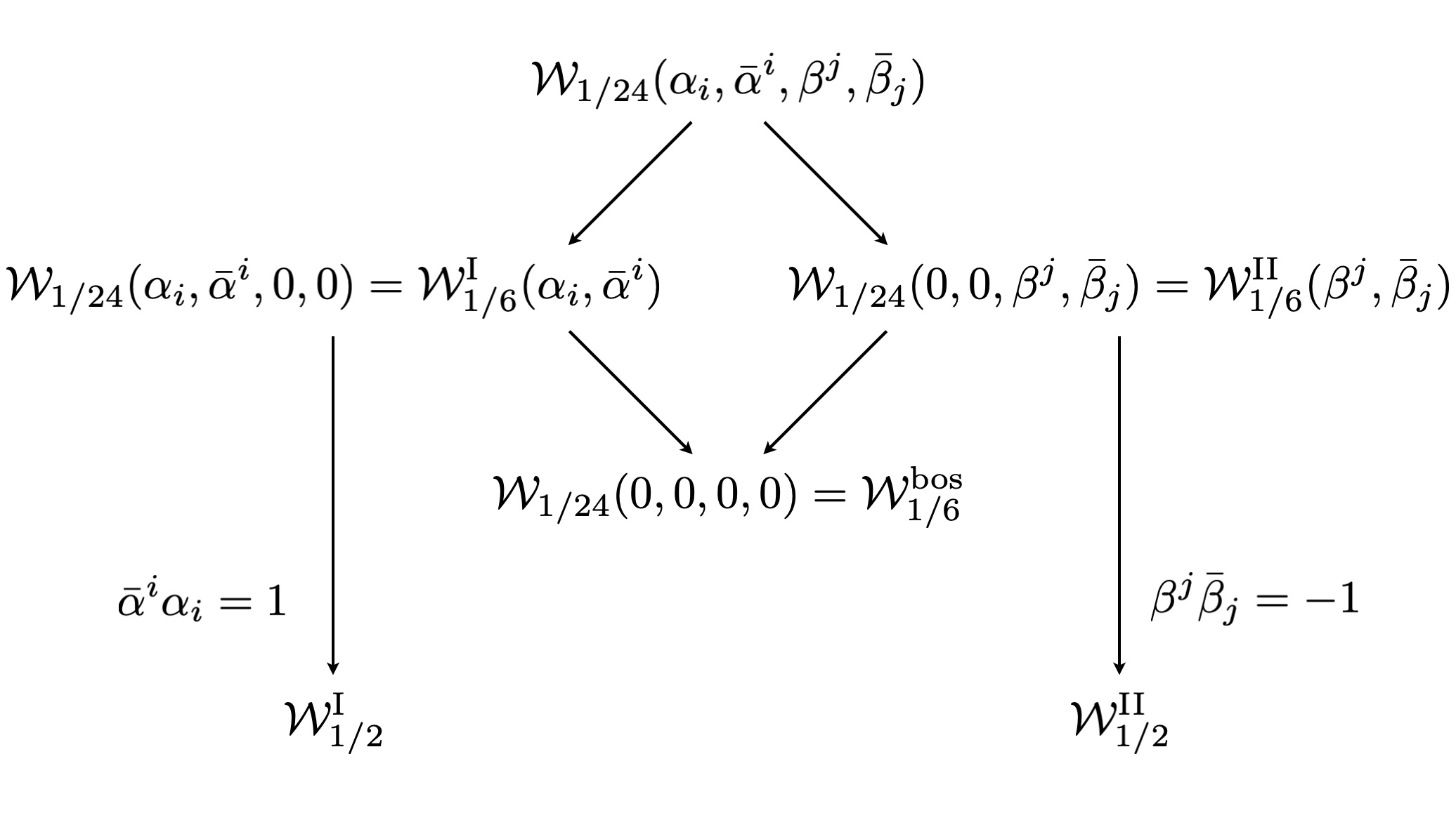
Figure 1: The interpolations among the various Wilson loops considered in this paper.

At the classical level all Wilson loops in figure 1 are cohomologically equivalent, i.e. their expressions differ by a ${\cal Q}$-exact term, where ${\cal Q}$ is one of the preserved supercharges. In principle, this would imply that their vacuum expectation values (VEVs) should be all equal and independent of the parameters. However, this is true for instance for operators supported along straight lines, but it is no longer true on the circle, due to the well-known conformal anomaly gross and framing effects. In fact, while supersymmetric localization requires framing 1, the regularization scheme we employ, namely dimensional regularization, is alternative to framing regularization and corresponds to framing 0. This is the reason why the circular VEVs that we are going to compute carry a non-trivial dependence on the parameters, so providing interpolating BPS (enriched) flows.

We compute the vacuum expectation value of this $1/24$ BPS circular loop, for generic values of the parameters, up to two loops in perturbation theory at weak coupling. The way we do it is by mapping this problem to the computation of the two-point function of certain auxiliary fields living on the one-dimensional theory along the Wilson loop contour. This is something that has been done in the past Samuel:1978iy ; Gervais:1979fv for ordinary Wilson loops, but we extend it to the case at hand, namely for Wilson loops defined in terms of superconnections. In particular, compared to the previous applications, in which the one-dimensional theory only contained a Fermi field, we have a theory with both commuting and anticommuting fields. The final planar-limit result for the Wilson loop VEV is given by

$$\langle{\mathcal{W}}_{1/24}\rangle=1-\frac{\pi^{2}}{6k^{2}}\left[N_{1}^{2}+N_{2}^{2}-4N_{1}N_{2}-3N_{1}N_{2}(\bar{\alpha}^{i}\alpha_{i}-\beta^{j}\bar{\beta}_{j}-1)^{2}\right]+{\cal O}\left(\frac{1}{k^{3}}\right)\,.$$ (1.1)

Here $N_{1}$ and $N_{2}$ are the ranks of the two gauge fields of the $U(N_{1})_{k}\times U(N_{2})_{-k}$ ABJ(M) theory, and $k$ is the Chern-Simons level. From this expression one obtains the VEVs of the $1/6$ BPS bosonic (all parameters equal to zero) and $1/6$ BPS fermionic operators (alphas or betas equal to zero), as well as of the $1/2$ BPS fermionic operator (last term in the square bracket equal to zero).

The coupling parameters undergo a non-trivial renormalization, leading to non-vanishing $\beta$-functions

$$\beta_{\alpha_{k}}=\frac{g^{2}}{4\pi}(N_{1}+N_{2})\,(\bar{\alpha}^{i}\alpha_{i}+\beta^{j}\bar{\beta}_{j}-1)\alpha_{k}\,,\qquad\beta_{\beta^{k}}=\frac{g^{2}}{4\pi}(N_{1}+N_{2})(\bar{\alpha}^{i}\alpha_{i}+\beta^{j}\bar{\beta}_{j}+1)\beta^{k}\,,$$ (1.2)

with similar expressions for the barred quantities. This shows that the Wilson loop parameters can be seen as marginally relevant deformations, triggering an RG flow from a UV fixed point represented by the $1/6$ BPS bosonic Wilson loop of ABJ(M) towards the $1/2$ BPS loop ${\mathcal{W}}_{1/2}^{\text{I}}$. Such a flow is presented in figure 13.

This has a nice interpretation in terms of defects. In fact, it is well known that the bosonic $1/6$ BPS and fermionic $1/6$ and $1/2$ BPS operators describe one-dimensional superconformal theories (SCFTs) given by local operators inserted on the Wilson loop contour. Instead, the new $1/24$ BPS operator supports a defect which is no longer (super)conformal, as it does not preserve enough supersymmetries and the contour dependence of the scalar couplings breaks conformality.

In this framework the RG flows depicted in figure 13 can be interpreted as connecting different (super)conformal defects seated at the fixed points. Flowing along the green line of that figure we reach a non-trivial IR fixed point. In the defect theory at the UV fixed point we compute the anomalous dimension of the parametric perturbation and consistently find a small negative value, thus confirming that it corresponds to a marginally relevant deformation.

Finally, from (1.1) and the $\beta$-functions we also establish a g-theorem, relating the VEVs of the Wilson loops corresponding to the UV and IR fixed points of the flows

$$\log\langle{\mathcal{W}}_{1/6}^{\textrm{bos}}\rangle>\log\langle{\mathcal{W}}_{1/2}^{\textrm{I}}\rangle\,,$$ (1.3)

similarly to what has been done for Wilson loops in four dimensions in Cuomo:2021rkm ; Beccaria:2021rmj , with the main difference being that our flows are BPS, as stressed above.

As mentioned already above, the comparison of the Wilson loop VEV (1.1) with the result coming from a matrix model computation Kapustin:2009kz ; Marino:2009jd requires taking into account framing issues, see chapter 6 of Drukker:2019bev for a review. The regularization scheme employed in our perturbative computation amounts in fact to computing the VEV at framing $f=0$, whereas the matrix model computation yields a result valid for $f=1$. Moreover, at framing one the VEVs of all loops of figure 1 coincide, as these are all cohomologically equivalent operators. This is clearly not true for (1.1), which is obtained at framing zero. Note, in particular, how this VEV depends explicitly on the alpha and beta parameters of the deformation, which are not present in the definition of the matrix model insertion corresponding to these operators. The relation between the VEVs of ${\mathcal{W}}_{1/24}$ at different framings is encoded in a phase, which we find empirically from our two-loop results to be given by

$$\langle{\cal W}_{1/24}\rangle_{f=1}=\frac{N_{1}e^{\frac{i\pi}{k}(N_{1}-(\bar{\alpha}^{i}\alpha_{i}-\beta^{j}\bar{\beta}_{j})N_{2})}+N_{2}\,e^{\frac{i\pi}{k}((\bar{\alpha}^{i}\alpha_{i}-\beta^{j}\bar{\beta}_{j})N_{1}-N_{2})}}{N_{1}+N_{2}}\langle{\cal W}_{1/24}\rangle_{f=0}\,.$$ (1.4)

We expect this phase to receive corrections at higher order in perturbation theory, similarly to what happens for the $1/6$ BPS bosonic operator Bianchi:2016yzj .

In this paper we also introduce a new operator: a $1/12$ BPS latitude Wilson loop defined in terms of an extra parameter, a latitude angle, along the lines of what has been done in ${\mathcal{N}}=4$ super Yang-Mills in Drukker:2007dw ; Drukker:2007yx ; Drukker:2007qr and in three-dimensional theories in Cardinali:2012ru ; Bianchi:2014laa and Drukker:2020dvr . In a forthcoming publication CPTT , we will generalize to this new setting the investigation of the present paper.

This paper is organized as follows. In section 2 we introduce the $1/24$ BPS circular Wilson loop, which is going to be the main character of our analysis, as well as the $1/12$ BPS latitude Wilson loop to be considered in the future. These operators are defined in terms of either traces or supertraces of superconnections. The former formulation simplifies the perturbative analysis while the latter is more natural for superconnections, so we discuss how to go from one to the other. In section 3 we consider an auxiliary problem in terms of one-dimensional fields which is suitable for studying the renormalization of the parameters of the $1/24$ BPS Wilson loop. This allows us to compute the $\beta$-functions of the Wilson loop parameters. In section 4 we finally compute the vacuum expectation value of the $1/24$ BPS circular Wilson loop up to two loops in perturbation theory. This is the main result of this paper, together with the evaluation of the $\beta$-functions. In section 5 we collect and discuss our results. Specifically, we describe the RG flows among the different operators of figure 1 and plot an explicit example, we study the defect SCFT living on the Wilson loop, we establish the g-theorem mentioned above, and we compare the Wilson loop VEV with a matrix model computation. Finally, we conclude that section with some outlook. We collect some technical aspects in a series of appendices. In appendix A we discuss our notation and conventions. In appendix B we derive the generalization of the one-dimensional auxiliary field method to Wilson loops defined in terms of superconnections. In appendix C we detail the computation of the various Feynman diagrams considered in the main text.

The reader who is not interested in technical details may skip section 3 and go directly to section 4.3.

2 Theory and supersymmetric loops

The field content of ABJ(M) can be depicted in terms of a quiver diagram as the one shown in figure 2. It includes two gauge fields, $A$ and $\hat{A}$, with respective gauge groups $U(N_{1})$ and $U(N_{2})$. The matter sector has $SU(4)$ R-symmetry and is composed of scalars $C_{I}$ and fermions $\bar{\psi}^{I}$, $I=\{1,2,3,4\}$, in the $(\Box,\bar{\Box})$ representation of $U(N_{1})\times U(N_{2})$. By conjugation there are also $\bar{C}^{I}$ and $\psi_{I}$ in $(\bar{\Box},\Box)$.

Figure 2: Quiver diagram of ABJ(M) theory. Below each node we include the level of the respective copy of the Chern-Simons action.

Wilson loops preserving some amount of the 24 supercharges of the theory can be constructed by allowing for couplings to scalar bilinears. In this case the usual gauge connection $A$ is promoted to a bosonic connection ${\mathcal{A}}$. Besides that, there is also the possibility of adding fermi fields, in which case the bosonic connection is further promoted to a superconnection ${\mathcal{L}}$ Drukker:2009hy . Recently, the structure of these operators started being unravelled Drukker:2019bev through the understanding that they are related via

$${\mathcal{L}}={\mathcal{L}}_{0}+i{\mathcal{Q}}G+G^{2}\,.$$ (2.1)

The quantity ${\mathcal{L}}_{0}$ is a composite bosonic connection complemented by a constant shift in one of the entries

$${\mathcal{L}}_{0}=\begin{pmatrix}{\mathcal{A}}+c&&0\\ 0&&\hat{\mathcal{A}}\end{pmatrix}\,.$$ (2.2)

The supercharge ${\mathcal{Q}}$ is a suitable linear combination of supercharges preserved by ${\mathcal{L}}_{0}$, and $G$ is an off-diagonal matrix comprised of scalars. These appear through a set of constant complex parameters that we denote as $\alpha_{i},\bar{\alpha}^{i},\beta^{j},\bar{\beta}_{j}$ (with $i=1,2$ and $j=3,4$), though they are not complex conjugates of each other. The construction (2.1) is such that ${\mathcal{Q}}$ is always preserved by ${\mathcal{L}}$, but one may find extra preserved supercharges depending on particular values of the parameters in $G$.

Below we consider two possible operators built from different choices of ${\mathcal{L}}_{0}$. The first one is the $1/24$ BPS circular loop, the protagonist of the present analysis, and the second one is the $1/12$ BPS latitude loop of ABJ(M), which is going to be studied in detail in a future publication CPTT . The construction of the latter is to a great extent parallel to the $\theta$-deformation considered in Drukker:2020dvr , with the difference that what we mean by ‘latitude’ here is an actual geometric latitude of the contour $x^{\mu}$ of the loop, instead of simply an internal $\theta$-deformation in the space of the couplings.

2.1 1/24 BPS circular Wilson loop

The first operator that we are going to consider is supported along the circle

$$x^{\mu}=(0,\cos\tau,\sin\tau)\,.$$ (2.3)

Its bosonic components can be separately charged under each node of the quiver

$${\mathcal{W}}^{\textrm{bos}} =\operatorname{Tr}{\mathcal{P}}\exp\left(-i\oint{\mathcal{A}}\,d\tau\right)\,,\qquad{\mathcal{A}}=A_{\mu}\dot{x}^{\mu}-\frac{2\pi i}{k}|\dot{x}|M_{J}^{\ I}C_{I}\bar{C}^{J}\,,$$ (2.4)

$$\hat{\mathcal{W}}^{\textrm{bos}} =\operatorname{Tr}{\mathcal{P}}\exp\left(-i\oint\hat{\mathcal{A}}\,d\tau\right)\,,\qquad\hat{\mathcal{A}}=\hat{A}_{\mu}\dot{x}^{\mu}-\frac{2\pi i}{k}|\dot{x}|M_{J}^{\ I}\bar{C}^{J}C_{I}\,.$$

When $M_{J}^{\ I}=\operatorname{diag}(-1,-1,1,1)$, they preserve the set of supercharges

$$Q_{12}^{+}-iS_{12}^{+}\,,\quad Q_{12}^{-}+iS_{12}^{-}\,,\quad Q_{34-}+iS_{34-}\,,\quad Q_{34+}-iS_{34+}\,,$$ (2.5)

and are therefore $1/6$ BPS operators Drukker:2008zx ; Chen:2008bp ; Kluson:2008zrv ; Rey:2008bh .

Their fermionic counterpart can be derived using the prescription outlined above. In this case, we take the supercharge ${\mathcal{Q}}$ to be given by the linear combination

$${\mathcal{Q}}\equiv(Q_{12}^{+}-iS_{12}^{+})+(Q_{34+}-iS_{34+})\,.$$ (2.6)

The constant shift is implemented in the composite bosonic connection ${\mathcal{L}}_{0}$ such that $c=\frac{1}{2}$ and the $G$ matrix includes all four scalars of the theory as

$$G=\begin{pmatrix}0&&\bar{\alpha}^{1}C_{1}+\bar{\alpha}^{2}C_{2}+e^{-i\tau}(\beta^{3}C_{3}+\beta^{4}C_{4})\\ \alpha_{1}\bar{C}^{1}+\alpha_{2}\bar{C}^{2}+e^{i\tau}(\bar{\beta}_{3}\bar{C}^{3}+\bar{\beta}_{4}\bar{C}^{4})&&0\end{pmatrix}\,.$$ (2.7)

Plugging this in (2.1) we find that the resulting superconnection ${\mathcal{L}}$ can be explicitly written as

$${\mathcal{L}}=\begin{pmatrix}{\mathcal{A}}^{\prime}+\frac{1}{2}&&\eta\,(\bar{\alpha}^{1}\bar{\psi}^{2}-\bar{\alpha}^{2}\bar{\psi}^{1})+e^{-i\tau}\xi\,(\beta^{3}\bar{\psi}^{4}-\beta^{4}\bar{\psi}^{3})\\ \xi\,(\alpha_{1}\psi_{2}-\alpha_{2}\psi_{1})+e^{i\tau}\eta\,(\bar{\beta}_{3}\psi_{4}-\bar{\beta}_{4}\psi_{3})&&\hat{{\mathcal{A}}}^{\prime}\end{pmatrix}\,,$$ (2.8)

where the commuting spinors $\eta$ and $\xi$ are

$$\eta^{\alpha}=\sqrt{\frac{2\pi i}{k}}(1,-ie^{-i\tau})^{\alpha}\,,\qquad\xi^{\alpha}=\sqrt{\frac{2\pi i}{k}}(-ie^{i\tau},1)^{\alpha}\,.$$ (2.9)

The diagonal entries are primed because now the scalar coupling matrix $M_{J}^{\ I}$ is such that it receives the contribution coming from $G^{2}$, i.e. it is

$$M_{J}^{\ I}=\begin{pmatrix}-1+2\bar{\alpha}^{1}\alpha_{1}&&2\bar{\alpha}^{1}\alpha_{2}&&2e^{i\tau}\bar{\alpha}^{1}\bar{\beta}_{3}&&2e^{i\tau}\bar{\alpha}^{1}\bar{\beta}_{4}\\ 2\bar{\alpha}^{2}\alpha_{1}&&-1+2\bar{\alpha}^{2}\alpha_{2}&&2e^{i\tau}\bar{\alpha}^{2}\bar{\beta}_{3}&&2e^{i\tau}\bar{\alpha}^{2}\bar{\beta}_{4}\\ 2e^{-i\tau}\beta^{3}\alpha_{1}&&2e^{-i\tau}\beta^{3}\alpha_{2}&&1+2\beta^{3}\bar{\beta}_{3}&&2\beta^{3}\bar{\beta}_{4}\\ 2e^{-i\tau}\beta^{4}\alpha_{1}&&2e^{-i\tau}\beta^{4}\alpha_{2}&&2\beta^{4}\bar{\beta}_{3}&&1+2\beta^{4}\bar{\beta}_{4}\end{pmatrix}\,.$$ (2.10)

The resulting operator,

$${\cal W}=\operatorname{sTr}{\mathcal{P}}\exp\left(-i\oint{\mathcal{L}}\,d\tau\right)\,,$$ (2.11)

preserves ${\mathcal{Q}}$. Following the proposal of drukker2020bps , it can be represented in terms of a quiver diagram as the one shown in figure 3.

Figure 3: The quiver diagram of the $1/24$ BPS Wilson loop in ABJ(M). Following the notation of drukker2020bps , a squiggly circle, like the one on the left here, represents a node whose bosonic connection is shifted by the constant $c$. The couplings to (anti-)chiral fields are denoted by solid (dashed) arrows.

As to the best of our knowledge this is the first time that such an operator is presented, we find it enlightening to stop and make a few comments about it before proceeding. First of all we notice that in the quiver of figure 3 solid arrows point both into and out of the squiggly node. From the analysis in Drukker:2020dvr , one can conclude that only ${\mathcal{Q}}$ is preserved, generically, and the loop is therefore 1/24 BPS.

Particular subcases of supersymmetry enhancement can be read off directly from the quiver structure. We know Drukker:2020dvr that when solid arrows point only into the squiggly node, all supercharges originally preserved by ${\mathcal{L}}_{0}$ are preserved by ${\mathcal{L}}$ and the resulting operator is $1/6$ BPS. To be explicit, when only $\alpha_{i},\bar{\alpha}^{i}$ parameters appear in $G$, see (2.7), the corresponding operator can be depicted in terms of a quiver diagram as in figure 4. In this case $G$ breaks only one $SU(2)$ R-symmetry subgroup of ${\mathcal{L}}_{0}$. Moreover, at the particular point $\bar{\alpha}^{i}\alpha_{i}=1$ the resulting loop enjoys extra $SU(3)$ symmetry and becomes $1/2$ BPS. On the other hand, for the case where only the $\beta^{j},\bar{\beta}_{j}$ parameters appear in $G$, it is useful to employ the gauge where the constant shift (and therefore the squigglyness of the corresponding quiver diagram) lies in the second node. In this case $G$ loses the awkward $e^{\pm i\tau}$ phases and the resulting operator can be depicted as in figure 4. This corresponds to $G$ breaking the other $SU(2)$ R-symmetry subgroup of ${\mathcal{L}}_{0}$ and at the particular point where $\beta^{j}\bar{\beta}_{j}=-1$, $SU(3)$ symmetry is restored and the loop is $1/2$ BPS. This is summarized in figure 1.

The particular cases outlined above recover the original analysis proposed in the second chapter of Drukker:2019bev , where the authors propose $G$’s that can be comprised of $\{C_{1},\bar{C}^{1},C_{2},\bar{C}^{2}\}$ or of $\{C_{3},\bar{C}^{3},C_{4},\bar{C}^{4}\}$. Our construction is therefore a generalization of that and corresponds to the most generic BPS operator one can build out of ${\mathcal{L}}_{0}$. All previously known examples can be derived from it through appropriate choices of the parameters.

Figure 4: Branches of $1/6$ BPS loops breaking different $SU(2)$ R-symmetries of ${\mathcal{L}}_{0}$.

Finally, seen from a different perspective, by viewing ABJ(M) as the orbifold of ${\mathcal{N}}=4$, the operator outlined above corresponds to the $1/16$ BPS operator appearing in figure 5 of Drukker:2020dvr , now specialized to ABJ(M).

2.2 1/12 BPS latitude Wilson loops

The latitude operators are supported along

$$x^{\mu}=(\sin\theta,\cos\theta\cos\tau,\cos\theta\sin\tau)\,.$$ (2.12)

Their bosonic representatives are still written as (2.4), but this time with

$$M_{J}^{\ I}=\begin{pmatrix}-\cos\theta&&0&&e^{-i\tau}\sin\theta&&0\\ 0&&-1&&0&&0\\ e^{i\tau}\sin\theta&&0&&\cos\theta&&0\\ 0&&0&&0&&1\end{pmatrix}\,.$$ (2.13)

This form of $M$ is such that the resulting loops are invariant under

$$\cos\frac{\theta}{2}\bigg{(}Q_{12}^{+}-ie^{-i\theta}S_{12}^{+}\bigg{)} -i\sin\frac{\theta}{2}\bigg{(}Q_{23}^{-}+ie^{-i\theta}S_{23}^{-}\bigg{)}\,,$$ (2.14)

$$\cos\frac{\theta}{2}\bigg{(}Q_{34+}-ie^{i\theta}S_{34+}\bigg{)} -i\sin\frac{\theta}{2}\bigg{(}Q_{14-}+ie^{i\theta}S_{14-}\bigg{)}\,.$$

As before, we follow the prescription (2.1) to construct the fermionic counterparts. We take the supercharge ${\mathcal{Q}}$ to be given by the sum of the supercharges above. Then the analysis of possible scalars to include in $G$ is parallel to the $\theta\neq 0$ discussion of Drukker:2020dvr . We find that $C_{2},\bar{C}^{2}$ and $C_{4},\bar{C}^{4}$ can not be included simultaneously due to the non-periodicity of boundary conditions that can not be fixed by means of a gauge transformation. To be precise, the superconnection would transform as the supercovariant derivative of

$$\begin{pmatrix}0&&\bar{\alpha}^{2}C_{2}+e^{-i\tau\cos\theta}\beta^{4}C_{4}\\ \alpha_{2}\bar{C}^{2}+e^{i\tau\cos\theta}\bar{\beta}_{4}\bar{C}^{4}&&0\end{pmatrix}\,,$$ (2.15)

which does not have well-behaved boundary conditions. As for the inclusion of $C_{1},\bar{C}^{1}$ and $C_{3},\bar{C}^{3}$, we find that it requires promoting the superconnection to a $3\times 3$ supermatrix and taking a cover of the quiver of the theory. Since this goes beyond the scope of our present discussion, we leave such possibility to the future.

We consider, therefore, two possible loops built out of $G$ coupling either to $C_{2},\bar{C}^{2}$ or to $C_{4},\bar{C}^{4}$. Both options are represented in figure 5, where the squigglyness of the nodes now stands for a constant shift of $c=\frac{\cos\theta}{2}$.

Figure 5: Branches of $1/12$ BPS latitude loops. Points where supersymmetry is enhanced correspond to $\alpha^{2}\bar{\alpha}_{2}=-\bar{\beta}^{4}\beta_{4}=1$, where an $SU(2)$ subgroup of R-symmetry is restored and the operators become $1/6$ BPS.

For brevity, we focus here on the explicit construction of the first branch. Its composite bosonic connection has a constant shift lying in the first node and the final form of the superconnection is

$${\mathcal{L}}^{\theta}=\begin{pmatrix}{\mathcal{A}}^{{}^{\prime}}+\frac{\cos\theta}{2}&&-\bar{\alpha}^{2}\eta\left(\cos\frac{\theta}{2}\bar{\psi}^{1}-\sin\frac{\theta}{2}e^{i\tau}\bar{\psi}^{3}\right)\\ -\alpha_{2}\xi\left(\cos\frac{\theta}{2}\psi_{1}-\sin\frac{\theta}{2}e^{-i\tau}\psi_{3}\right)&&\hat{\mathcal{A}}^{{}^{\prime}}\end{pmatrix}\,,$$ (2.16)

with the scalar coupling now given by

$$M_{J}^{\ I}=\begin{pmatrix}-\cos\theta&&0&&e^{-i\tau}\sin\theta&&0\\ 0&&-1+2\bar{\alpha}^{2}\alpha_{2}&&0&&0\\ e^{i\tau}\sin\theta&&0&&\cos\theta&&0\\ 0&&0&&0&&1\end{pmatrix}\,.$$ (2.17)

At the particular point where $\bar{\alpha}^{2}\alpha_{2}=1$, an $SU(2)$ subgroup of R-symmetry is preserved. The loop is invariant under the supercharges (2.14) and the ones obtained by swapping the $2\leftrightarrow 4$ indices. This is the $1/6$ BPS latitude operator introduced in Bianchi:2014laa and further studied in Bianchi:2018bke ; Griguolo_2021 .

2.3 Removing the constant shift

The constant shift $c$ in (2.2) is useful in the definition of the operators (see chapter 2 of Drukker:2019bev ). Its presence gives rise to a manifestly reparametrisation invariant operator. Moreover, Wilson loops with this shift are (super)gauge invariant without the need for an additional twist matrix Cardinali:2012ru and can be defined as the supertrace of a superconnection, as in (2.11), rather than with a trace, as in the original construction of Drukker:2009hy . However, the presence of this shift makes the perturbative calculation more intricate (see chapter 5 of Drukker:2019bev ), so we find it helpful to remove it before proceeding to the next section.

To illustrate the procedure we will take the latitude operator. The $\theta\rightarrow 0$ limit of the analysis below reproduces the circular case. We make a $U(N_{1})$ gauge transformation in order to remove the constant shift from the first node,

$$A_{\mu}\dot{x}^{\mu}+\frac{\cos\theta}{2}\quad\longrightarrow\quad A_{\mu}\dot{x}^{\mu}+\frac{d\Lambda}{d\tau}+\frac{\cos\theta}{2}=A_{\mu}\dot{x}^{\mu}+\text{boundary terms}\,,$$ (2.18)

where boundary terms may arise from the discontinuity of $\Lambda$ on the circle. Precisely, we choose

$$\Lambda=-\frac{\cos\theta}{2}\tau+\Delta\sum_{n\in\mathbb{Z}}\theta(\tau-2\pi n)\,,$$ (2.19)

where a constant $\Delta$ has been introduced, so to insure that $\int_{0}^{2\pi}d\tau\frac{d\Lambda}{d\tau}$ vanishes. Requiring

$$0=\int_{0}^{2\pi}d\tau\ \frac{d\Lambda}{d\tau}=\int_{0}^{2\pi}d\tau\left(-\frac{\cos\theta}{2}+\Delta\,\delta(\tau-2\pi)\right)=-\pi\cos\theta+\Delta\,,$$ (2.20)

we obtain $\Delta=\pi\cos\theta$. Therefore, the original gauge term $(A_{\mu}\dot{x}^{\mu}+\frac{\cos\theta}{2})$ in the superconnection is now replaced by $(A_{\mu}\dot{x}^{\mu}+\pi\cos{\theta}\,\delta(\tau-2\pi))$.

Taking this delta function contribution into account, we recover the twist matrix ${\mathcal{T}}$

$${\mathcal{P}}\exp\left(-i\int_{2\pi-\epsilon}^{2\pi+\epsilon}{\mathcal{L}}\,d\tau\right)\rightarrow\exp\left(-i\begin{pmatrix}\pi\cos\theta&0\\ 0&0\end{pmatrix}\right)=\begin{pmatrix}e^{-i\pi\cos\theta}&0\\ 0&1\end{pmatrix}\equiv{\mathcal{T}}\,.$$ (2.21)

In the circular case this is simply ${\mathcal{T}}=\operatorname{diag}(-1,1)$. In the latitude case, in order to follow the same conventions of Bianchi:2014laa , we rescale it such that

$${\mathcal{T}}\equiv\begin{pmatrix}e^{-i\pi(\cos\theta)/2}&0\\ 0&e^{i\pi(\cos\theta)/2}\end{pmatrix}\,.$$ (2.22)

The gauge transformation we have performed in order to remove the constant shift acts on the matter fields as

$$\begin{split}&\bar{\psi}^{I}\to\bar{\psi}^{I}e^{-i\Lambda}=\bar{\psi}^{I}e^{i\cos\theta\,\tau/2}\,,\qquad\qquad\psi_{I}\to\psi_{I}e^{i\Lambda}=\psi_{I}e^{-i\cos\theta\,\tau/2}\,,\\ &\bar{C}^{I}\to\bar{C}^{I}e^{-i\Lambda}=\bar{C}^{I}e^{i\cos\theta\,\tau/2}\,,\qquad\qquad C_{I}\to C_{I}e^{i\Lambda}=C_{I}e^{-i\cos\theta\,\tau/2}\,.\end{split}$$ (2.23)

The diagonal elements of the superconnection remain unchanged, while the fermionic entries gain extra phases. For the circular $1/24$ BPS operator these are

$$\begin{split}\bar{f}&=e^{i\tau/2}\,\eta\left(\bar{\alpha}^{1}\bar{\psi}^{2}-\bar{\alpha}^{2}\bar{\psi}^{1}\right)+e^{-i\tau/2}\xi\,(\beta^{3}\bar{\psi}^{4}-\beta^{4}\bar{\psi}^{3})\,,\\ f&=e^{-i\tau/2}\,\xi\,\left(\alpha_{1}\psi_{2}-\alpha_{2}\psi_{1}\right)+e^{i\tau/2}\eta\,(\bar{\beta}_{3}\psi_{4}-\bar{\beta}_{4}\psi_{3})\,,\end{split}$$ (2.24)

while for the latitude $1/12$ BPS operator they are

$$\bar{f}^{\theta} =-e^{i\cos\theta\,\tau/2}\,\eta\,\bar{\alpha}^{2}\left(\cos\frac{\theta}{2}\bar{\psi}^{1}-\sin\frac{\theta}{2}e^{i\tau}\bar{\psi}^{3}\right),$$ (2.25)

$$f^{\theta} =-e^{-i\cos\theta\,\tau/2}\,\xi\,\alpha_{2}\left(\cos\frac{\theta}{2}\psi_{1}-\sin\frac{\theta}{2}e^{-i\tau}\psi_{3}\right)\,.$$

Therefore, the final form of the superconnection is

$${\mathcal{L}}=\begin{pmatrix}{\mathcal{A}}&\bar{f}\\ f&\hat{\mathcal{A}}\end{pmatrix}\,,$$ (2.26)

without the constant shift in the first diagonal block, unlike (2.2), and similarly for the case with $\theta\neq 0$.

The Wilson loop operator is now written as

$${\mathcal{W}}={\mathcal{R}}^{-1}\,\operatorname{sTr}{\cal P}\left(e^{-i\oint{\cal L}d\tau}{\mathcal{T}}\right)\,,$$ (2.27)

where we have introduced the normalization factor ${\mathcal{R}}=\operatorname{sTr}({\mathcal{T}})$. In particular, from now on, we will refer to the circular Wilson loop as

$${\mathcal{W}}=\frac{W}{N_{1}+N_{2}},\qquad W\equiv\text{Tr}\,{\cal P}\exp\left(-i\oint{\cal L}\,d\tau\right),$$ (2.28)

with the ${\cal L}$ in (2.26).

3 Renormalization

3.1 1D effective field theory for the Wilson loop VEV

At weak coupling, the standard procedure for computing the vacuum expectation value of a Wilson loop is ordinary perturbation theory. In the functional approach, this amounts to expanding the exponential of the interaction part of the bulk action in powers of the coupling constant and performing contractions with the Wilson loop expansion using Feynman rules for the bulk theory.

In the QCD context, in the 80’s Samuel Samuel:1978iy , Gervais and Neveu Gervais:1979fv proposed an alternative method to study Wilson loop operators, based on the formulation of a one-dimensional effective field theory. Subsequently, this method was further developed and heavily exploited to study the renormalization of composite operators Arefeva:1980zd ; CRAIGIE1981204 ; Dorn:1986dt .

The method makes use of auxiliary one-dimensional fermions and can be briefly summarized as follows. Suppose that in a given gauge theory one wants to evaluate a generic Wilson loop supported along a contour ${\mathcal{C}}$,

$$W[{\mathcal{C}}]=\operatorname{Tr}{\mathcal{P}}\exp\left(-i\int_{\mathcal{C}}{\mathcal{L}}\,d\tau\right)\,.$$ (3.1)

In this expression ${\mathcal{L}}$ may be the ordinary gauge connection $A$ or one of the bosonic connections ${\mathcal{A}}$ given in (2.4). In any case, one can write the perturbative expansion of the operator as

$$\begin{split}W[{\cal C}]&=\operatorname{Tr}\left(1+\sum_{k=1}^{\infty}\frac{(-i)^{k}}{k!}{\mathcal{P}}\int_{{\mathcal{C}}}d\tau_{1}d\tau_{2}\dots d\tau_{k}\,{\mathcal{L}}(\tau_{1}){\mathcal{L}}(\tau_{2})\dots\mathcal{L}(\tau_{k})\right)\\ &=\operatorname{Tr}\left(1+\sum_{k=1}^{\infty}(-i)^{k}\int_{{\mathcal{C}}}d\tau_{1}d\tau_{2}\dots d\tau_{k}\,\theta(\tau_{k}-\tau_{k-1})\dots\theta(\tau_{2}-\tau_{1}){\mathcal{L}}(\tau_{1}){\mathcal{L}}(\tau_{2})\dots\mathcal{L}(\tau_{k})\right)\,.\end{split}$$ (3.2)

The idea is to interpret $\theta(\tau_{i}-\tau_{j})$ as the propagator of an auxiliary fermionic field $z$ living on the Wilson loop contour, whose interaction with the rest of the fields is dictated by ${\mathcal{L}}$. Taking the $z$ field in the fundamental representation of the gauge group, its action is chosen to be

$$S_{\textrm{eff}}=S+\int d\tau\,\bar{z}(\tau)\left[\partial_{\tau}+i{\mathcal{L}}\right]z(\tau)\,,$$ (3.3)

where $S$ is the action of the underlying gauge theory. Performing the Gaussian $z$-integral in the generating functional, it can be shown that for a contour ${\mathcal{C}}_{12}$ connecting two points parametrized by $\tau_{1},\tau_{2}$ one has CRAIGIE1981204 ; Dorn:1986dt

$$\langle W[{\mathcal{C}}_{12}]\rangle=\left\langle\operatorname{Tr}{\mathcal{P}}\exp\left(-i\int_{\tau_{2}}^{\tau_{1}}{\mathcal{L}}\,d\tau\right)\right\rangle=\langle z(\tau_{2})\bar{z}(\tau_{1})\rangle\,,$$ (3.4)

where

$$\langle z(\tau_{2})\bar{z}(\tau_{1})\rangle=\int[{\mathcal{D}}z{\mathcal{D}}\bar{z}]\,z(\tau_{2})\bar{z}(\tau_{1})\,e^{-S_{\textrm{eff}}}.$$ (3.5)

Therefore, the expectation value of $W$ is nothing but the two-point function of the one-dimensional theory defined on it.

This method could be naturally generalized to study renormalization properties of Wilson loops in supersymmetric theories. Here, we propose a generalization that captures the expectation value of operators in the ABJ(M) theory.

Since in this theory Wilson loops are defined in terms of supermatrices, the natural way to proceed is to replace the one-dimensional auxiliary $z$ fermion with a Grassmann odd supermatrix

$$\Psi=\begin{pmatrix}z&\varphi\\ \tilde{\varphi}&\tilde{z}\end{pmatrix}\,,\qquad\bar{\Psi}=\begin{pmatrix}\bar{z}&\bar{\tilde{\varphi}}\\ \bar{\varphi}&\bar{\tilde{z}}\end{pmatrix}\,,$$ (3.6)

where $z$ ($\tilde{z}$) and $\varphi$ ($\tilde{\varphi}$) are a spinor and a scalar, respectively, in the fundamental representation of $U(N_{1})$ ($U(N_{2})$). We then look for an effective theory such that the ABJ(M) Wilson loop VEV (2.27) can be computed as a two-point function of the one-dimensional fields. To this end, we consider the following action

$$S_{\textrm{eff}}=S_{\textrm{ABJ(M)}}+\int d\tau\,\operatorname{Tr}\left(\bar{\Psi}{\mathcal{D}}_{\tau}\Psi\right)\,,$$ (3.7)

where $S_{\textrm{ABJ(M)}}$ is the ABJ(M) action (see (A.2)) and ${\mathcal{D}}_{\tau}=\partial_{\tau}+i{\mathcal{L}}(\tau)$, ${\mathcal{L}}$ being the Wilson loop superconnection. It is then easy to prove that

$$\langle W[{\mathcal{C}}_{12}]\rangle=\,\langle\operatorname{Tr}\Psi(\tau_{2})\bar{\Psi}(\tau_{1})\rangle\,,$$ (3.8)

where the vacuum functional on the right-hand side includes the integrations over both the bulk fields and the one-dimensional $\Psi,\bar{\Psi}$ supermatrices, weighted by the action (3.7). We provide more details about this derivation in appendix B.

We focus here on the circular Wilson loop defined in section 2.1, while postponing the investigation of the latitude operator of section 2.2 to a future publication CPTT . Expanding the matrix product and defining for simplicity $g=\sqrt{\frac{2\pi}{k}}$, the effective action can be written explicitly as

$$\begin{split}S_{\textrm{eff}}=S_{\textrm{ABJ(M)}}+\int d\tau\Big{[}&\bar{\varphi}D_{\tau}\varphi+\bar{\tilde{\varphi}}\hat{D}_{\tau}\tilde{\varphi}+\bar{z}D_{\tau}z+\bar{\tilde{z}}\hat{D}_{\tau}\tilde{z}\\ &+i(\bar{\tilde{z}}f\varphi+\bar{\varphi}\bar{f}\tilde{z}+\bar{\tilde{\varphi}}fz+\bar{z}\bar{f}\tilde{\varphi})\Big{]}\,,\end{split}$$ (3.9)

where we have defined $D_{\tau}=\partial_{\tau}+i{\mathcal{A}}$ and $\hat{D}_{\tau}=\partial_{\tau}+i\hat{\mathcal{A}}$. ${\mathcal{A}}$, $\hat{{\mathcal{A}}}$, $f$ and $\bar{f}$ are the even and odd elements of the Wilson loop superconnection, see (2.26). The covariant $\tau$-derivatives give rise to the usual minimal coupling between the one-dimensional fields and the bulk gauge vectors, plus quartic interactions with bulk scalar bilinears. We have not inserted the explicit expressions of $f,\bar{f}$, which can be found in (2.25). At this stage, it is only important to take into account that these couplings are proportional to one power of $g$. The tree-level propagators of the one-dimensional fields are

$$=\langle z^{i}(\tau_{1})\bar{z}_{j}(\tau_{2})\rangle =\delta_{j}^{i}\,\theta(\tau_{1}-\tau_{2})\,,$$ (3.10)

$$=\langle{\tilde{z}}^{\hat{i}}(\tau_{1})\bar{\tilde{z}}_{\hat{j}}(\tau_{2})\rangle =\delta_{\hat{j}}^{\hat{i}}\,\theta(\tau_{1}-\tau_{2})\,,$$

$$=\langle\varphi^{i}(\tau_{1})\bar{\varphi}_{j}(\tau_{2})\rangle =\delta_{j}^{i}\,\theta(\tau_{1}-\tau_{2})\,,$$

$$=\langle\tilde{\varphi}^{\hat{i}}(\tau_{1})\bar{\tilde{\varphi}}_{\hat{j}}(\tau_{2})\rangle =\delta_{\hat{j}}^{\hat{i}}\,\theta(\tau_{1}-\tau_{2})\,.$$

3.2 Renormalization scheme

We now focus on the perturbative evaluation of the two-point function (3.8) for the one-dimensional theory. This first requires investigating whether the one-dimensional fields and the couplings undergo a non-trivial renormalization, due to short distance divergences arising on the loop.

For each one-dimensional field $\phi=\{\varphi,\tilde{\varphi},z,\tilde{z}\}$ the corresponding renormalization functions are defined as $\phi=Z_{\phi}^{-\frac{1}{2}}\phi_{0}$, where $\phi_{0}$ stands for the bare quantity. We note that since the action (3.9) is invariant under the formal exchanges $z\leftrightarrow\varphi$ and $\tilde{z}\leftrightarrow\tilde{\varphi}$, we can set $Z_{z}=Z_{\varphi}$ and $Z_{\tilde{z}}=Z_{\tilde{\varphi}}$. As we are going to prove, the field function renormalization is sufficient to cancel UV divergent contributions to both the kinetic terms and the interaction vertices between auxiliary fields and gauge connections, i.e. the $\bar{\phi}A_{\mu}\dot{x}^{\mu}\phi$ vertices. This is consistent with the expectation that the addition of the auxiliary action in (3.7) does not affect the UV finiteness of the ABJ(M) theory ($A_{\mu}$ does not renormalize).

As follows from the definition of $f,\bar{f}$ and $M_{I}^{\ J}$ in (2.24) and (2.10), respectively, the fermionic interactions (as for instance $\bar{\tilde{z}}f\varphi$) and the quartic couplings with the scalar bilinears contain the $g$ coupling and the $\alpha_{i},\bar{\alpha}^{i},\beta^{j},\bar{\beta}_{j}$ parameters as further couplings.

For the renormalization of the fermionic interactions we define

$$\begin{split}&(\bar{\alpha}^{i})_{0}\,Z^{1/2}_{\tilde{z}}Z_{\varphi}^{1/2}=(\bar{\alpha}^{i})_{0}\,Z^{1/2}_{z}Z_{\tilde{\varphi}}^{1/2}=Z_{\bar{\alpha}^{i}}\,\bar{\alpha}^{i}\,,\\ &(\alpha_{i})_{0}\,Z^{1/2}_{\tilde{z}}Z_{\varphi}^{1/2}=(\alpha_{i})_{0}\,Z^{1/2}_{z}Z_{\tilde{\varphi}}^{1/2}=Z_{\alpha_{i}}\,\alpha_{i}\,,\\ &(\beta^{j})_{0}\,Z^{1/2}_{\tilde{z}}Z_{\varphi}^{1/2}=(\beta^{j})_{0}\,Z^{1/2}_{z}Z_{\tilde{\varphi}}^{1/2}=Z_{\beta^{j}}\,\beta^{j}\,,\\ &(\bar{\beta}_{j})_{0}\,Z^{1/2}_{\tilde{z}}Z_{\varphi}^{1/2}=(\bar{\beta}_{j})_{0}\,Z^{1/2}_{z}Z_{\tilde{\varphi}}^{1/2}=Z_{\bar{\beta}_{j}}\,\bar{\beta}_{j}\,,\end{split}$$ (3.11)

where the subscript 0 denotes bare parameters and we have used that the ABJ(M) coupling does not renormalize, i.e. $g_{0}=g$. The scalar vertices of the form $M_{I}^{\ J}\bar{\phi}C_{J}\bar{C}^{I}\phi$ deserve more attention since the parametric dependence is hidden inside the scalar coupling matrix $M_{I}^{\ J}$. We set

$$Z_{\varphi}({M}_{I}^{\ J})_{0}=Z_{\varphi C}M_{I}^{\ J}\,,\qquad Z_{\tilde{\varphi}}({M}_{I}^{\ J})_{0}=Z_{\tilde{\varphi}C}M_{I}^{\ J}\,,$$ (3.12)

$$Z_{z}({M}_{I}^{\ J})_{0}=Z_{zC}M_{I}^{\ J}\,,\qquad Z_{\tilde{z}}\,({M}_{I}^{\ J})_{0}=Z_{\tilde{z}C}M_{I}^{\ J}\,,$$

where $({M}_{I}^{\ J})_{0}$ is the scalar coupling matrix expressed in terms of the bare parameters.

Using the standard BPHZ renormalization procedure, we write all renormalization functions as $Z=1+\delta$, where $\delta$ are the corresponding countertems. We then extract the Feynman rules from the one-dimensional Lagrangian written as the sum of a renormalized Lagrangian plus the counterterm part

$${\mathcal{L}}_{\textrm{1D}}={\mathcal{L}}^{\textrm{ren}}_{\textrm{1D}}+{\mathcal{L}}_{\textrm{1D}}^{\text{ct}}\,,$$ (3.13)

where ${\mathcal{L}}^{\textrm{ren}}_{\textrm{1D}}$ is given by (3.9) written in terms of renormalized quantities and the counterterms read

$$\begin{split}{\mathcal{L}}^{\text{ct}}_{\textrm{1D}}&=\sum_{\phi=\varphi,z}\left(\delta_{\phi}\,\bar{\phi}\partial_{\tau}\phi+\delta_{\phi}\,ig\bar{\phi}A_{\mu}\dot{x}^{\mu}\phi+\delta_{\phi C}\,g^{2}|\dot{x}|M_{I}^{\ J}\bar{\phi}C_{J}\bar{C}^{I}\phi\right)\\ &+\sum_{\tilde{\phi}=\tilde{\varphi},\tilde{z}}\left(\delta_{\tilde{\phi}}\,\bar{\tilde{\phi}}\partial_{\tau}\tilde{\phi}+\delta_{\tilde{\phi}}\,ig\bar{\tilde{\phi}}\hat{A}_{\mu}\dot{x}^{\mu}\tilde{\phi}+\delta_{\tilde{\phi}C}\,g^{2}|\dot{x}|M_{I}^{\ J}\bar{\tilde{\phi}}\bar{C}^{I}C_{J}\tilde{\phi}\right)\\ &+i\bar{\tilde{z}}\left(e^{-\frac{i\tau}{2}}\xi\left(\delta_{\alpha_{1}}\,\alpha_{1}\psi^{2}-\delta_{\alpha_{2}}\,\alpha_{2}\psi^{1}\right)+e^{\frac{i\tau}{2}}\eta\,(\delta_{\bar{\beta}_{3}}\,\bar{\beta}_{3}\psi^{4}-\delta_{\bar{\beta}_{4}}\,\bar{\beta}_{4}\psi^{3})\right)\varphi\\ &+i\bar{\tilde{\varphi}}\left(e^{-\frac{i\tau}{2}}\xi\left(\delta_{\alpha_{1}}\,\alpha_{1}\psi^{2}-\delta_{\alpha_{2}}\,\alpha_{2}\psi^{1}\right)+e^{\frac{i\tau}{2}}\eta\,(\delta_{\bar{\beta}_{3}}\,\bar{\beta}_{3}\psi^{4}-\delta_{\bar{\beta}_{4}}\,\bar{\beta}_{4}\psi^{3})\right)z\\ &+i\bar{\varphi}\left(e^{\frac{i\tau}{2}}\eta\left(\delta_{\bar{\alpha}^{1}}\,\bar{\alpha}^{1}\bar{\psi}^{2}-\delta_{\bar{\alpha}^{2}}\,\bar{\alpha}^{2}\bar{\psi}^{1}\right)+e^{-\frac{i\tau}{2}}\xi\,(\delta_{\beta^{3}}\,\beta^{3}\bar{\psi}^{4}-\delta_{\beta^{4}}\,\beta^{4}\bar{\psi}^{3})\right)\tilde{z}\\ &+i\bar{z}\left(e^{\frac{i\tau}{2}}\eta\left(\delta_{\bar{\alpha}^{1}}\,\bar{\alpha}^{1}\bar{\psi}^{2}-\delta_{\bar{\alpha}^{2}}\,\bar{\alpha}^{2}\bar{\psi}^{1}\right)+e^{-\frac{i\tau}{2}}\xi\,(\delta_{\beta^{3}}\beta^{3}\bar{\psi}^{4}-\delta_{\beta^{4}}\,\beta^{4}\bar{\psi}^{3})\right)\tilde{\varphi}\,,\end{split}$$ (3.14)

with obvious meanings of the $\delta$’s.

3.3 Evaluation of one-loop counterterms

We begin by investigating the structure of the counterterms at one loop. We tame short distance divergences arising from the evaluation of Feynman integrals by using dimensional regularization in $D=1-2\epsilon$ and a minimal subtraction scheme. We work in the large $N_{1},N_{2}$ limit.

Since we want to study the UV behavior of our one-dimensional theory, we work in the $\tau_{2}\to\tau_{1}$ limit, where $\tau$ parameterizes the curve on which the theory is defined. Therefore, any regular contour can be approximated, around a point, by a straight segment, such that $|\dot{x}|=1$ and $\dot{x}\cdot\ddot{x}=0$. In this limit, for a generic one-dimensional field $\phi$ we use the following approximation

$$\phi_{2}\simeq\phi_{1}+(\tau_{2}-\tau_{1})\dot{\phi}_{1}\,,$$ (3.15)

as well as the following expansion for the coordinates on the contour

$$\begin{split}&x^{\mu}_{2}\simeq x^{\mu}_{1}+(\tau_{2}-\tau_{1})\dot{x}^{\mu}_{1}\,,\qquad\dot{x}^{\mu}_{2}\simeq\dot{x}^{\mu}_{1}+(\tau_{2}-\tau_{1})\ddot{x}^{\mu}_{1}\,,\\ &\left(x_{2}-x_{1}\right)^{2}\simeq(\tau_{2}-\tau_{1})^{2}\,\dot{x}_{1}^{2}\,\left(1+(\tau_{2}-\tau_{1})\frac{\dot{x}_{1}\cdot\ddot{x}_{1}}{\dot{x}_{1}^{2}}\right)\,,\end{split}$$ (3.16)

To keep the discussion as clear as possible, we provide here details for the first few diagrams and collect the rest of the calculations in appendix C.

Corrections to the kinetic term

We begin by considering one-loop self-energy corrections to the $\langle\bar{z}z\rangle$ propagator of the one-dimensional theory. The contributing diagrams are drawn in figure 6 (we neglect tadpole diagrams, as they vanish in dimensional regularization).

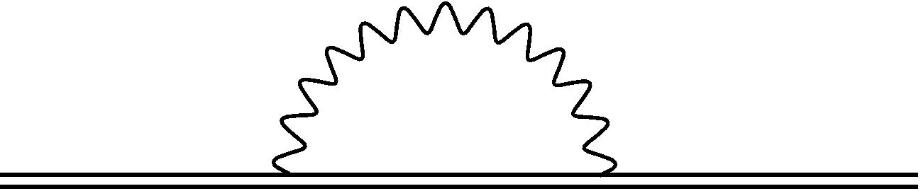
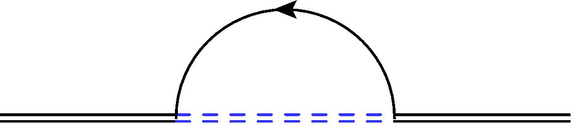
Figure 6: One-loop corrections to the fermionic propagator $\langle\bar{z}z\rangle$. Double straight lines represent $z$ and $\bar{z}$, blue double dashed lines are the one-dimensional $\tilde{\varphi}$ scalars, simple straight lines are ABJ(M) fermions, whereas wavy lines describe the ABJ(M) $U(N_{1})$ gauge field. Diagram (c) is the $\delta_{z}$ counterterm in (3.14).

The first diagram is the gauge field correction and gives rise to the following contribution

$$\Sigma^{\rm\ref{subfig:vertexcorrectiona}}_{z}=\int d\tau_{1}\int d\tau_{2}\,\bar{z}_{1}\,z_{2}\,\dot{x}_{1}^{\mu}\,\dot{x}_{2}^{\nu}\,\theta(\tau_{1}-\tau_{2})\langle A_{\mu}(\tau_{1})A_{\nu}(\tau_{2})\rangle\,.$$ (3.17)

However, inserting the explicit expression (A.4) for the gauge propagator and using the expansions (3.16), it is easy to see that in dimensional regularization this integral vanishes, due to the antisymmetry of the $\epsilon_{\mu\nu\rho}$ tensor.

The second diagram gives (we define $\tau_{12}\equiv\tau_{1}-\tau_{2}$)

$$\begin{split}\Sigma^{\rm\ref{subfig:vertexcorrectionb}}_{z}&=\int d\tau_{1}\int d\tau_{2}\left(i\bar{z}\bar{f}\tilde{\varphi}\right)(\tau_{1})\left(i\bar{\tilde{\varphi}}fz\right)(\tau_{2})\\ &=\bar{\alpha}^{i}\alpha_{i}\int d\tau_{1}\int^{\tau_{1}}d\tau_{2}\,\bar{z}_{1}\,z_{2}\,e^{\frac{i\tau_{12}}{2}}\eta_{\alpha}(\tau_{1})\xi^{\beta}(\tau_{2})\langle\bar{\psi}^{\alpha}(\tau_{1})\psi_{\beta}(\tau_{2})\rangle\\ &+\beta^{j}\bar{\beta}_{j}\int d\tau_{1}\int^{\tau_{1}}d\tau_{2}\,\bar{z}_{1}\,z_{2}\,e^{-\frac{i\tau_{12}}{2}}\xi_{\alpha}(\tau_{1})\eta^{\beta}(\tau_{2})\langle\bar{\psi}^{\alpha}(\tau_{1})\psi_{\beta}(\tau_{2})\rangle\,,\end{split}$$ (3.18)

where we have already used $\langle\tilde{\varphi}_{1}\bar{\tilde{\varphi}}_{2}\rangle=\theta(\tau_{1}-\tau_{2})$. Inserting the fermionic propagator (A.4), it explicitly reads

$$\begin{split}\Sigma^{\rm\ref{subfig:vertexcorrectionb}}_{z}&=i\bar{\alpha}^{i}\alpha_{i}\frac{\Gamma(\frac{3}{2}-\epsilon)}{2\pi^{\frac{3}{2}-\epsilon}}\int d\tau_{1}\int^{\tau_{1}}d\tau_{2}\,\bar{z}_{1}\,z_{2}\,e^{i\frac{\tau_{12}}{2}}\xi^{\alpha}(\tau_{2})(\gamma_{\mu})_{\alpha}^{\ \beta}\eta_{\beta}(\tau_{1})\frac{(x_{2}-x_{1})^{\mu}}{|x_{2}-x_{1}|^{3-2\epsilon}}\\ &+i\beta^{j}\bar{\beta}_{j}\frac{\Gamma(\frac{3}{2}-\epsilon)}{2\pi^{\frac{3}{2}-\epsilon}}\int d\tau_{1}\int^{\tau_{1}}d\tau_{2}\,\bar{z}_{1}\,z_{2}\,e^{-i\frac{\tau_{12}}{2}}\eta^{\alpha}(\tau_{2})(\gamma_{\mu})_{\alpha}^{\ \beta}\xi_{\beta}(\tau_{1})\frac{(x_{2}-x_{1})^{\mu}}{|x_{2}-x_{1}|^{3-2\epsilon}}\,.\end{split}$$ (3.19)

In the $\tau_{2}\to\tau_{1}$ limit, using the explicit expression for the $\xi,\eta$ spinors and the gamma matrices in (A.1), we can write

$$\begin{split}e^{i\frac{\tau_{12}}{2}}\xi^{\alpha}(\tau_{2})\,(\gamma_{\mu})_{\alpha}^{\ \beta}\,\eta_{\beta}(\tau_{1})\,(x_{2}-x_{1})^{\mu}&=-4ig^{2}\sin\frac{\tau_{12}}{2}\,\simeq\,-2ig^{2}(\tau_{1}-\tau_{2})\,,\\ e^{-i\frac{\tau_{12}}{2}}\eta^{\alpha}(\tau_{2})\,(\gamma_{\mu})_{\alpha}^{\ \beta}\,\xi_{\beta}(\tau_{1})\,(x_{2}-x_{1})^{\mu}&=-4ig^{2}\sin\frac{\tau_{12}}{2}\,\simeq\,-2ig^{2}(\tau_{1}-\tau_{2})\,.\end{split}$$ (3.20)

Expanding the rest of the integrand with (3.15), (3.16), the integral reduces to

$$\begin{split}\Sigma^{\rm\ref{subfig:vertexcorrectionb}}_{z}&=-g^{2}N_{2}\,(\bar{\alpha}^{i}\alpha_{i}+\beta^{j}\bar{\beta}_{j})\frac{\Gamma(\frac{3}{2}-\epsilon)}{\pi^{\frac{3}{2}-\epsilon}}\int d\tau_{1}\bar{z}_{1}\,\dot{z}_{1}\int^{\tau_{1}}d\tau_{2}\,(\tau_{1}-\tau_{2})^{-1+2\epsilon}+\cdots\\ &=-g^{2}\frac{N_{2}}{4\pi\epsilon}(\bar{\alpha}^{i}\alpha_{i}+\beta^{j}\bar{\beta}_{j})\int d\tau\,\bar{z}\,\partial_{\tau}z+\text{finite terms}\,,\end{split}$$ (3.21)

where in the first line dots indicate terms of the expansion which give rise to finite integrals, and in the second line we have extracted the divergent part for $\epsilon\to 0$.

Finally, the counterterm contribution is

$$\Sigma^{\rm\ref{subfig:vertexcorrectiond}}_{z}=-\delta_{z}\int d\tau\,\bar{z}\partial_{\tau}z\,.$$ (3.22)

Therefore the total correction to the $z,\bar{z}$ propagator $\Sigma_{z}$, given by the sum of all diagrams above, is

$$\Sigma_{z}=\left(-g^{2}\frac{N_{2}}{4\pi\epsilon}(\bar{\alpha}^{i}\alpha_{i}+\beta^{j}\bar{\beta}_{j})-\delta_{z}\right)\int d\tau\bar{z}\partial_{\tau}z\,.$$ (3.23)

Requiring the counterterm to cancel the divergence, we eventually find

$$Z_{z}=Z_{\varphi}=1-g^{2}\frac{N_{2}}{4\pi\epsilon}(\bar{\alpha}^{i}\alpha_{i}+\beta^{j}\bar{\beta}_{j})\,.$$ (3.24)

The same procedure can be applied to the tilde fields, obtaining similar contributions

$$Z_{\tilde{z}}=Z_{\tilde{\varphi}}=1-g^{2}\frac{N_{1}}{4\pi\epsilon}(\bar{\alpha}^{i}\alpha_{i}+\beta^{j}\bar{\beta}_{j})\,.$$ (3.25)

Corrections to the gauge-fermion vertex

We now consider one-loop corrections to the gauge-fermion vertex $S_{\bar{z}Az}=i\int d\tau\,\bar{z}A_{\mu}\dot{x}^{\mu}z$. The corresponding diagrams are summarized in figure 7. In the following we simply list the final result of each integral, referring to appendix C.1 for the details of the computation.

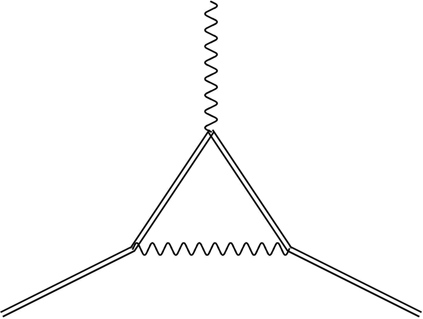
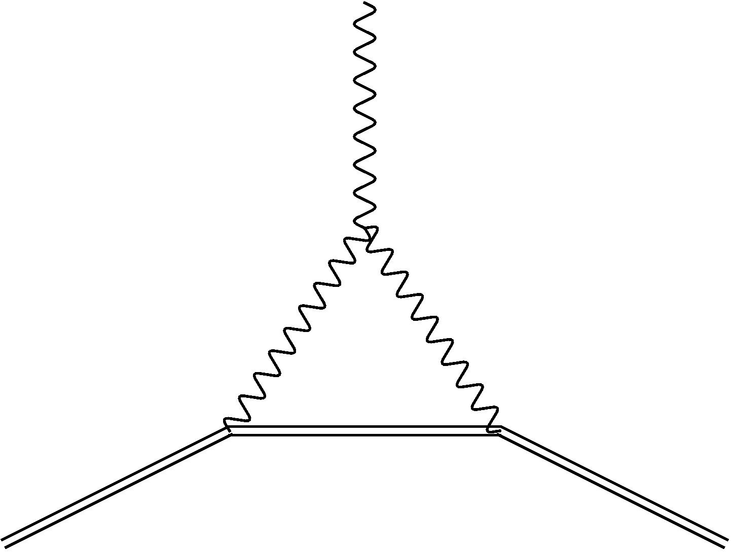
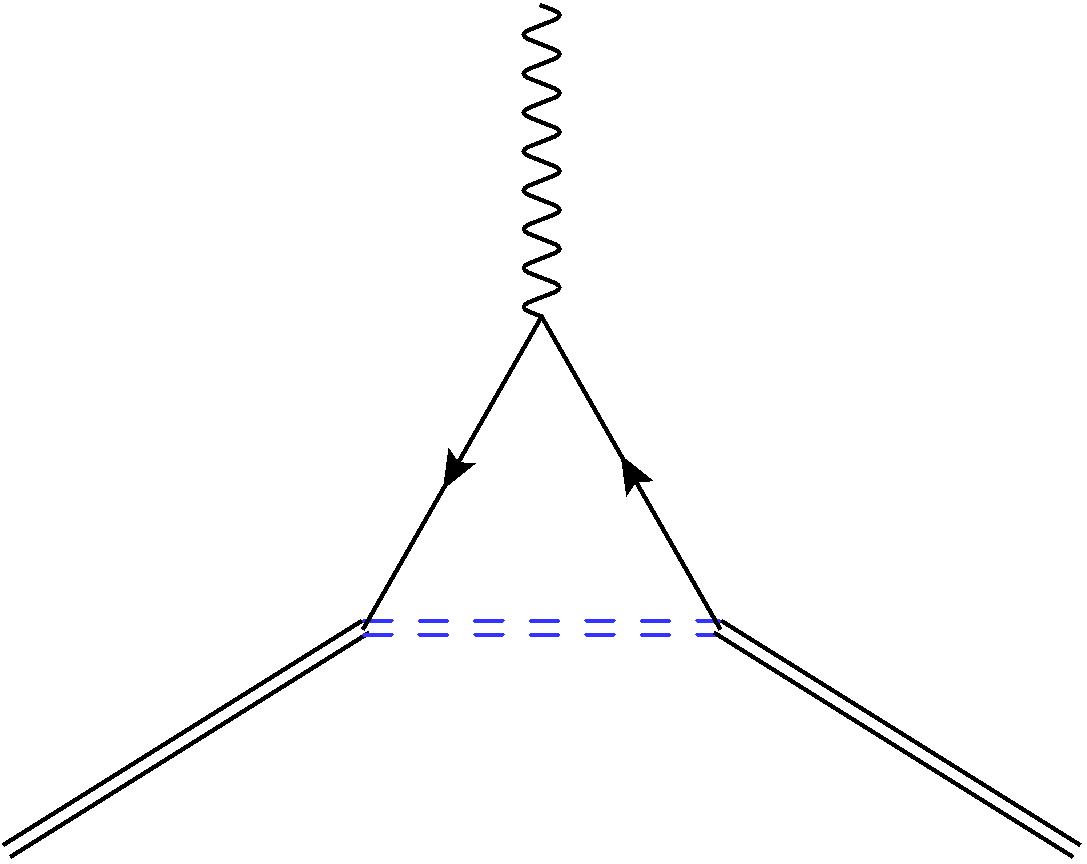
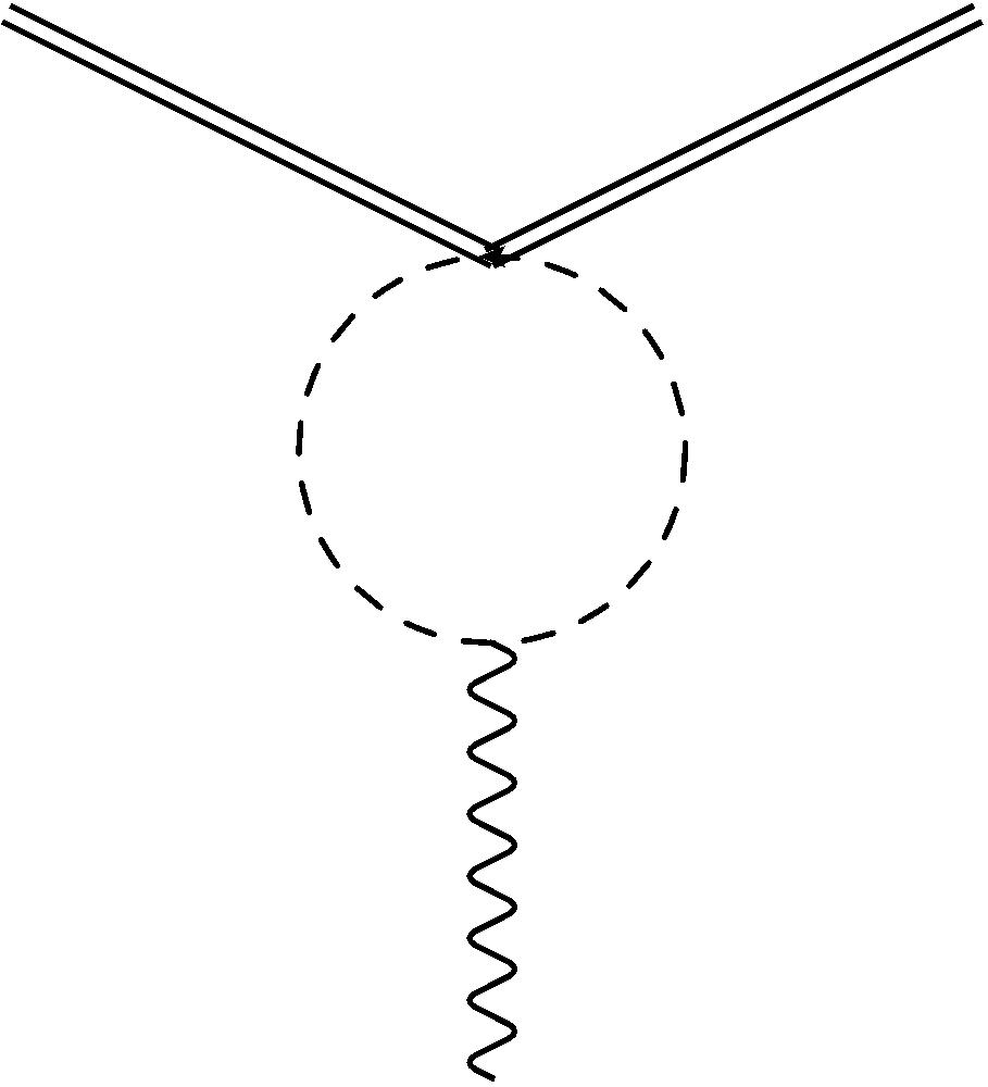
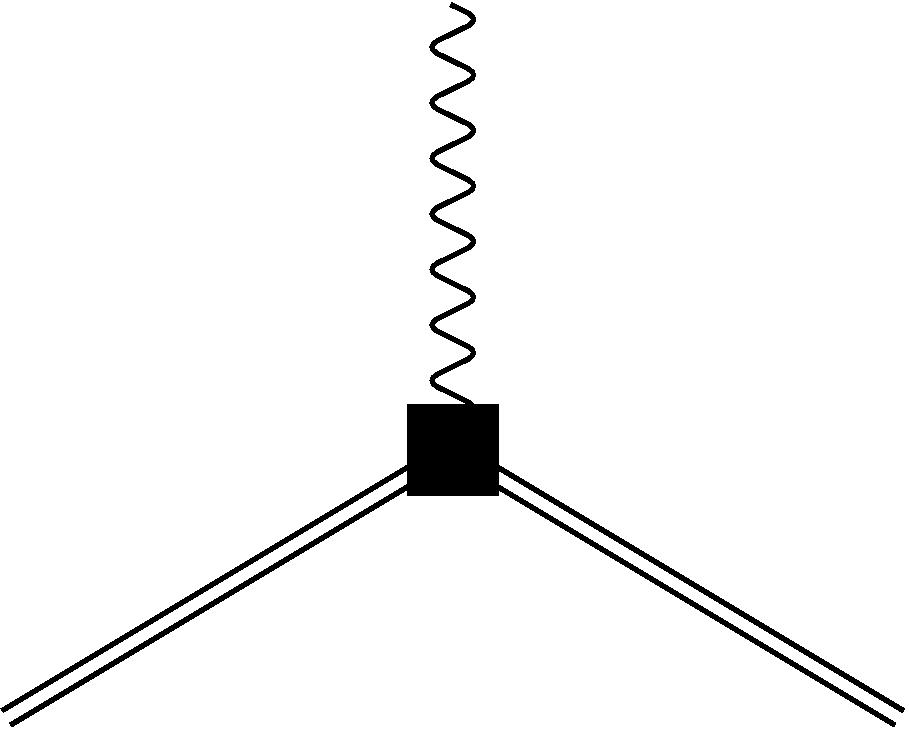
Figure 7: One-loop corrections of the $V_{\bar{z}Az}$ vertex. The blue double-dashed line describes the $\tilde{\varphi}$ propagator, while the single-dashed line describes the ABJM scalar fields $C_{I}$. The last diagram represents the $\delta_{z}$ counterterm.

To begin with, it is easy to see that diagram 7 does not contribute, due to planarity. In fact, using the expansions (3.16), the associated divergence turns out to be proportional to $\epsilon_{\mu\nu\rho}\dot{x}_{1}^{\mu}\dot{x}_{1}^{\nu}$.

For the same reason, as discussed in appendix C.1, the divergent contribution of diagram 7 also vanishes. This diagram contains the three gauge field vertex coming from the ABJ(M) action, $\frac{1}{3g^{2}}\epsilon^{\mu\nu\rho}\int d^{d}x\,\operatorname{Tr}(A_{\mu}A_{\nu}A_{\rho})$ (here $d=3-2\epsilon$). Therefore, it is proportional to the product of three epsilon tensors, one from the vertex and two from the gauge propagators. Using ordinary epsilon tensor algebra, this product can be reduced to a single epsilon, but eventually the remaining tensor is contracted with the same vector twice.

Diagram 7 is built using the gauge-fermion-fermion vertex from the original ABJ(M) action $-\int d^{d}x\operatorname{Tr}(g\bar{\psi}^{J}\gamma^{\mu}A_{\mu}\psi_{J})$. Its divergent contribution reads

$$\Gamma^{\rm\ref{subfig:gauge1c}}_{\text{gauge}}=-\frac{g^{2}N_{2}}{4\pi\epsilon}(\bar{\alpha}^{i}\alpha_{i}+\beta^{j}\bar{\beta}_{j})\int d\tau\ i\bar{z}A_{\mu}\dot{x}^{\mu}z\,.$$ (3.26)

Finally, diagram 7 contains the gauge-scalar vertex coming from minimal coupling in the ABJ(M) action, $i\int d^{d}x\,(A^{\mu}C_{I}\partial_{\mu}\bar{C}^{I}-\partial_{\mu}C_{I}\,\bar{C}^{I}A^{\mu})$. In Lorentz gauge this diagram turns out to be equal to zero, as shown in appendix C.1.

Summing all the contributions, the correction to the gauge vertex $\Gamma_{\text{gauge}}$ is eventually given by

$$\Gamma_{\text{gauge}}=\left(-\delta_{z}-\frac{g^{2}N_{2}}{4\pi\epsilon}(\bar{\alpha}^{i}\alpha_{i}+\beta^{j}\bar{\beta}_{j})\right)\int d\tau\,i\bar{z}A_{\mu}\dot{x}^{\mu}z\,.$$ (3.27)

Comparing with (3.24), we see that $\delta_{z}$ cancels exactly the divergence.

Following the same procedure for the $\bar{\tilde{z}}\hat{A}_{\mu}\tilde{z}$ vertex, we find that the result changes only by a color factor. Precisely, we obtain

$${\hat{\Gamma}}_{\text{gauge}}=\left(-\delta_{\tilde{z}}-\frac{g^{2}N_{1}}{4\pi\epsilon}(\bar{\alpha}^{i}\alpha_{i}+\beta^{j}\bar{\beta}_{j})\right)\int d\tau\,i\bar{\tilde{z}}\hat{A}_{\mu}\dot{x}^{\mu}{\tilde{z}}\,,$$ (3.28)

and $\delta_{\tilde{z}}$ in (3.25) cancels exactly this vertex divergence.

The same pattern holds also for the remaining gauge-boson vertices, i.e. $\bar{\varphi}A_{\mu}\dot{x}^{\mu}\varphi$ and $\bar{\tilde{\varphi}}A_{\mu}\dot{x}^{\mu}{\tilde{\varphi}}$.

Fermion vertex corrections

To compute the counterterm associated with the fermion vertex correction (last four lines in (3.14)), we first consider the coupling $i\bar{\tilde{z}}f\varphi$. Inserting the explicit expression (2.24) for $f$, this amounts to evaluating four different vertex structures, precisely

$$i\alpha_{1}e^{-i\tau/2}\xi\,\bar{\tilde{z}}\psi^{2}\varphi-i\alpha_{2}e^{-i\tau/2}\xi\,\bar{\tilde{z}}\psi^{1}\varphi+i\bar{\beta}_{3}e^{i\tau/2}\eta\,\bar{\tilde{z}}\psi^{4}\varphi-i\bar{\beta}_{4}e^{i\tau/2}\eta\,\bar{\tilde{z}}\psi^{3}\varphi\,,$$ (3.29)

with $\xi,\eta$ given in (2.9).

For all the structures, the typologies of diagrams to be considered are shown in figure 8. The ABJ(M) vertices $-\bar{\psi}^{I}\gamma^{\mu}\psi_{I}A_{\mu}$ and $\bar{\psi}^{I}\gamma^{\mu}\hat{A}_{\mu}\psi_{I}$ appear in 8 and 8, respectively. Since these vertices are diagonal in the fermion colors, the correction to the $\alpha_{1}$ and $\alpha_{2}$ vertices will be the same, as well as the ones for $\bar{\beta}_{3}$ and $\bar{\beta}_{4}$.

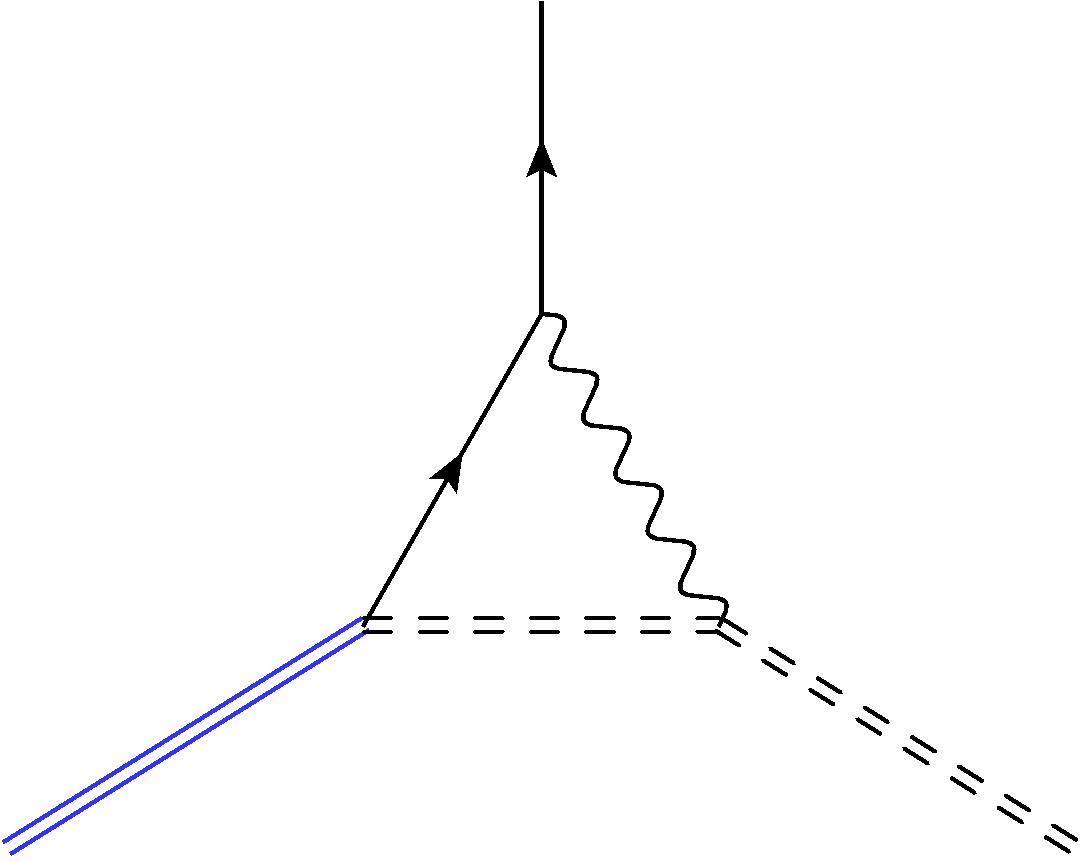
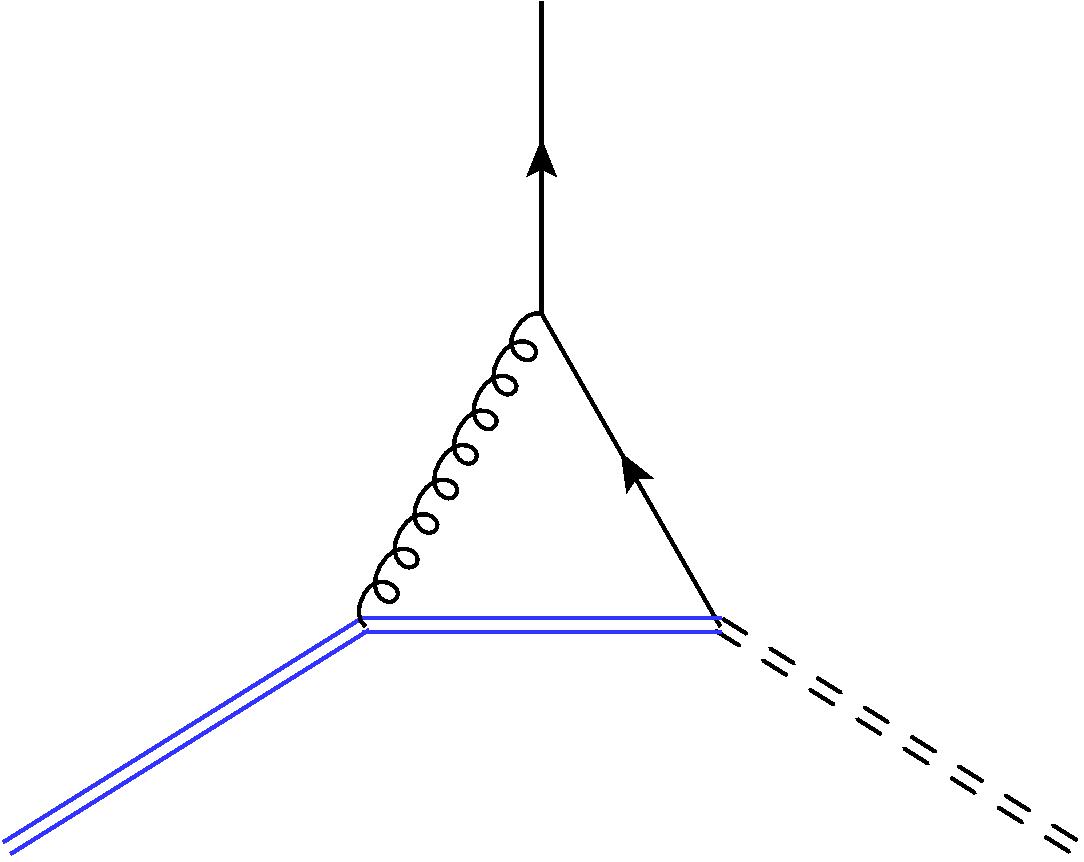
Figure 8: One-loop corrections to the $V_{\bar{\tilde{z}}f\varphi}$ vertex. Wavy lines correspond to $A_{\mu}$ propagators, whereas wiggly lines represent $\hat{A}_{\mu}$ propagators.

Considering first the corrections to the $\alpha_{i}$ vertices, from diagram 8 we obtain (the details are in appendix C.2)

$$\Gamma^{\rm\ref{subfig:fermion1a}}_{\text{fermion}}=\frac{g^{2}N_{1}}{8\pi\epsilon}i\int d\tau\bar{\tilde{z}}\left(\alpha_{1}e^{-i\tau/2}\xi\,\psi^{2}-\alpha_{2}\,e^{-i\tau/2}\xi\,\psi^{1}\right)\varphi\,.$$ (3.30)

For diagram 8 we find the same contribution with $N_{1}$ replaced by $N_{2}$.

Summing up the three diagrams, the one-loop correction to the $\alpha_{i}$ fermion vertices is given by

$$i\int d\tau\bar{\tilde{z}}\left[\left(\delta_{\alpha_{1}}+\frac{g^{2}(N_{1}+N_{2})}{8\pi\epsilon}\right)\alpha_{1}e^{-i\tau/2}\xi\,\psi^{2}-\left(\delta_{\alpha_{2}}+\frac{g^{2}(N_{1}+N_{2})}{8\pi\epsilon}\right)\alpha_{2}\,e^{-i\tau/2}\xi\,\psi^{1}\right]\varphi\,.$$ (3.31)

It is easy to check that performing the same computation for the fermionic vertices proportional to $\bar{f}$ in (2.24), we obtain the same corrections to the $\bar{\alpha}^{i}$ couplings. Consequently, we find

$$Z_{\bar{\alpha}^{i}}=Z_{\alpha_{i}}=1-\frac{g^{2}(N_{1}+N_{2})}{8\pi\epsilon},\qquad\quad i=1,2\,.$$ (3.32)

Similarly, for the $\beta^{j},\bar{\beta}_{j}$ couplings in (3.29) we obtain

$$Z_{\beta^{j}}=Z_{\bar{\beta}_{j}}=1+\frac{g^{2}(N_{1}+N_{2})}{8\pi\epsilon},\qquad\quad j=3,4\,.$$ (3.33)

The different sign compared with (3.32) comes from the different couplings accompanying $\bar{\alpha}^{i},\alpha_{i}$ and $\beta^{j},\bar{\beta}_{j}$ parameters.

Scalar vertex corrections

Now we study the corrections to the scalar vertex $S_{\varphi C}=g^{2}M_{I}^{\ J}\int d\tau\bar{\varphi}C_{J}\bar{C}^{I}\varphi$, as the prototype of the four-point vertices in (3.9). This vertex requires particular attention since the components of $M_{I}^{\ J}$ are functions of the $\alpha_{i},\bar{\alpha}^{i},\beta^{j},\bar{\beta}_{j}$ parameters. In the most general case, the $1/24$ BPS matrix of (2.10), the parameters appear in all the components, and this renders the computation rather involved. However, considering the particular case $\bar{\alpha}^{2}\alpha_{2}=\beta^{3}\bar{\beta}_{3}=\beta^{4}\bar{\beta}_{4}=0$ is sufficient to compute the desired corrections, while simplifying considerably the calculations. We will then stick to this case.

At leading order in the gauge colors, the diagrams that contribute to the four-point vertex are depicted in figure 9. Further non-vanishing diagrams could be drawn, which however lead to subleading corrections proportional to double-trace vertices. Since we work at large $N_{1},N_{2}$, we neglect them.

Details on the computation of each diagram are presented separately in appendix C.3. Here, we list only the results.

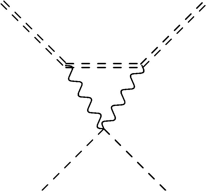
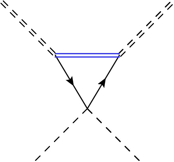
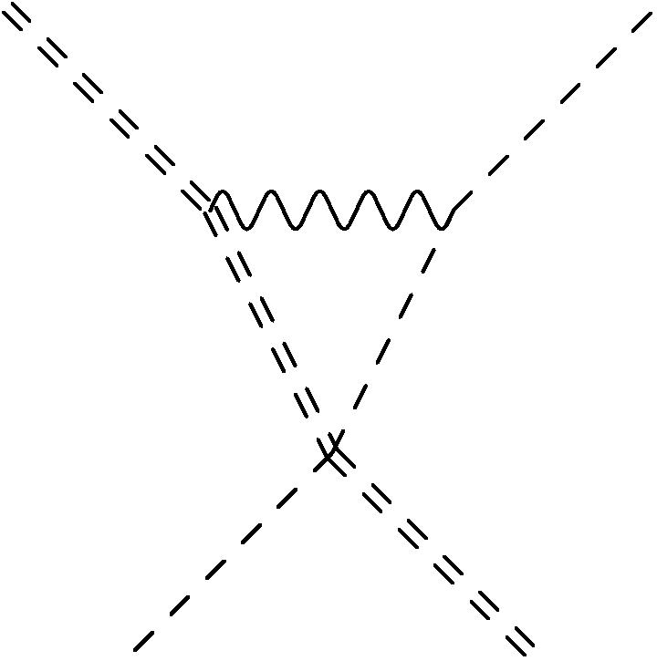
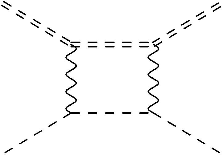
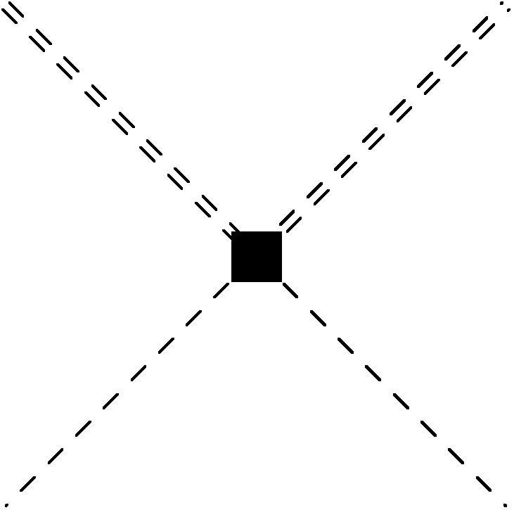
Figure 9: Leading one-loop corrections of the $V_{\bar{\varphi}C\bar{C}\varphi}$ vertex. The last diagram corresponds to the $\delta_{\varphi C}$ counterterm.

From the first two diagrams we obtain

$$\begin{split}&\Gamma^{\rm\ref{subfig:scalarvertexa}}_{\text{scalar}}=-g^{4}\frac{N_{1}}{8\pi\epsilon}M_{I}^{\ K}M_{K}^{\ J}\int d\tau\,\bar{\varphi}\,C_{J}\bar{C}^{I}\varphi\,,\\ &\Gamma^{\rm\ref{subfig:scalarvertexb}}_{\text{scalar}}=g^{4}\frac{N_{1}}{8\pi\epsilon}\int d\tau\,\bar{\varphi}\,C_{I}\bar{C}^{I}\varphi\,.\end{split}$$ (3.34)

Diagram 9 involves the Yukawa couplings appearing in the last two lines of the ABJ(M) action in (A.2). It can be built either using the $2g^{2}C_{I}\bar{C}^{J}\bar{\psi}^{I}\psi_{J}$ vertex or the $-g^{2}C_{I}\bar{C}^{I}\bar{\psi}^{J}\psi_{J}$ one. The two corresponding contributions read respectively

$$\begin{split}&\Gamma^{\rm\ref{subfig:scalarvertexc},1}_{\text{scalar}}=-g^{4}\frac{N_{2}}{2\pi\epsilon}\bar{\alpha}^{1}\alpha_{1}\int d\tau\bar{\varphi}\,C_{2}\bar{C}^{2}\varphi\,,\\ &\Gamma^{\rm\ref{subfig:scalarvertexc},2}_{\text{scalar}}=g^{4}\frac{N_{2}}{4\pi\epsilon}\bar{\alpha}^{1}\alpha_{1}\int d\tau\bar{\varphi}\,C_{I}\bar{C}^{I}\varphi\,.\end{split}$$ (3.35)

Therefore, we can summarize the result from this diagram as

$$\Gamma^{\rm\ref{subfig:scalarvertexc}}_{\text{scalar}}=g^{4}\frac{N_{2}}{4\pi\epsilon}\bar{\alpha}^{1}\alpha_{1}\begin{pmatrix}1&0&0&0\\ 0&-1&0&0\\ 0&0&1&0\\ 0&0&0&1\end{pmatrix}_{\!\!\,I}^{\ J}\int d\tau\,\bar{\varphi}C_{J}\bar{C}^{I}\varphi\,.\,$$ (3.36)

Finally, we move on to diagrams 9 and 9. Working in Lorentz gauge, it is easy to see that the corresponding contributions are not divergent. In fact, we can always integrate by parts the $\partial_{\mu}$ derivatives coming from the ABJ(M) vertices on the external $C_{I},\bar{C}^{I}$ lines. As a consequence, the integrand is finite for dimensional reasons.

Summing all the contributions, we eventually obtain

$$0=g^{2}\left[\delta_{\varphi C}M_{I}^{\ J}-g^{2}\frac{N_{1}}{8\pi\epsilon}\left(M_{I}^{\ K}M_{K}^{\ J}-\delta_{I}^{J}\right)+g^{2}\frac{N_{2}}{4\pi\epsilon}\bar{\alpha}^{1}\alpha_{1}(\delta_{I}^{J}-2\delta_{I}^{2}\delta^{J}_{2})\right]\int d\tau\,\bar{\varphi}C_{J}\bar{C}^{I}\varphi\,.$$ (3.37)

This implies that

$$Z_{\varphi C}M_{I}^{\ J}=(1+\delta_{\varphi C})M_{I}^{\ J}=M_{I}^{\ J}+\frac{g^{2}}{4\pi\epsilon}\bar{\alpha}^{1}\alpha_{1}\left[-N_{2}(\delta_{I}^{J}-2\delta_{I}^{2}\delta^{J}_{2})+2N_{1}(\bar{\alpha}^{1}\alpha_{1}-1)\delta_{I}^{1}\delta^{J}_{1}\right]\,.$$ (3.38)

From the definition (LABEL:eq:Mren), for the scalar coupling renormalization we can write

$$({M}_{I}^{\ J})_{0}=\frac{Z_{\varphi C}}{Z_{\varphi}}M_{I}^{\ J}=M_{I}^{\ J}+\frac{g^{2}}{4\pi\epsilon}\bar{\alpha}^{1}\alpha_{1}\left[-N_{2}(\delta_{I}^{J}-2\delta_{I}^{2}\delta^{J}_{2})+2N_{1}(\bar{\alpha}^{1}\alpha_{1}-1)\delta_{I}^{1}\delta^{J}_{1}+N_{2}M_{I}^{\ J}\right]\,.$$ (3.39)

The term at order $g^{2}$ on the right-hand side is zero for $I=J=2,3,4$, whereas for $I=J=1$ we obtain

$$(\bar{\alpha}^{1}\alpha_{1})_{0}=\bar{\alpha}^{1}\alpha_{1}\left[1+\frac{g^{2}}{4\pi\epsilon}(N_{1}+N_{2})(\bar{\alpha}^{1}\alpha_{1}-1)\right]\,,$$ (3.40)

where on the left-hand side the subscript indicates the product of the two bare parameters. This result is consistent with the $\alpha_{1},\bar{\alpha}^{1}$ renormalization that we have already discussed.

3.4 $\beta$-functions

Having determined the renormalization functions, we can now compute the one-loop $\beta$-functions for the parameters. To this end, we first recall that the definition of the bare parameters are given in (LABEL:eq:parren). Collecting the results for the renormalization functions found in the previous sections,

$$\begin{split}Z_{z}^{1/2}&=1-g^{2}\frac{N_{2}}{8\pi\epsilon}(\bar{\alpha}^{i}\alpha_{i}+\beta^{j}\bar{\beta}_{j})\,,\\ Z_{\tilde{\varphi}}^{1/2}&=1-g^{2}\frac{N_{1}}{8\pi\epsilon}(\bar{\alpha}^{i}\alpha_{i}+\beta^{j}\bar{\beta}_{j})\,,\\ Z_{\bar{\alpha}^{i}}=Z_{\alpha_{i}}&=1-\frac{g^{2}(N_{1}+N_{2})}{8\pi\epsilon}\,,\\ Z_{\beta^{j}}=Z_{\bar{\beta}_{j}}&=1+\frac{g^{2}(N_{1}+N_{2})}{8\pi\epsilon}\,,\end{split}$$ (3.41)

and plugging them there, we find

$$\begin{split}&(\alpha_{k})_{0}=\left(1+\frac{g^{2}}{8\pi\epsilon}\,(N_{1}+N_{2})(\bar{\alpha}^{i}\alpha_{i}+\beta^{j}\bar{\beta}_{j}-1)\right)\alpha_{k}\qquad k=1,2\,,\\ &(\bar{\alpha}^{k})_{0}=\left(1+\frac{g^{2}}{8\pi\epsilon}\,(N_{1}+N_{2})(\bar{\alpha}^{i}\alpha_{i}+\beta^{j}\bar{\beta}_{j}-1)\right)\bar{\alpha}^{k}\,,\\ &(\bar{\beta}_{l})_{0}=\left(1+\frac{g^{2}}{8\pi\epsilon}\,(N_{1}+N_{2})(\bar{\alpha}^{i}\alpha_{i}+\beta^{j}\bar{\beta}_{j}+1)\right)\bar{\beta}_{l}\;\,\qquad l=3,4\,,\\ &(\beta^{l})_{0}=\left(1+\frac{g^{2}}{8\pi\epsilon}\,(N_{1}+N_{2})(\bar{\alpha}^{i}\alpha_{i}+\beta^{j}\bar{\beta}_{j}+1)\right)\beta^{l}\,.\end{split}$$ (3.42)

As already mentioned, if we set $\bar{\alpha}^{2}=\alpha_{2}=\bar{\beta}_{j}=\beta^{j}=0$ and consider the product $(\bar{\alpha}^{1}\alpha_{1})_{0}$, we obtain exactly the expression (3.40) coming from the renormalization of the four-point scalar vertices. This is a non-trivial check of our renormalization procedure.

The one-dimensional theory under investigation possesses nine dimensionless coupling constants $g_{a}=(g^{2},\alpha_{i},\bar{\alpha}^{i},\beta^{j},\bar{\beta}_{j})$, with the new indices $a,b,\ldots$ running over these nine couplings. In dimensional regularization with $d=3-2\epsilon$, the $\alpha_{i},\bar{\alpha}^{i},\beta^{j},\bar{\beta}_{j}$ parameters remain dimensionless, while $g^{2}$ acquires dimension $\Delta_{g^{2}}=2\epsilon$.

Expressing the bare coupling constants $(g_{a})_{0}$ as a function of the renormalized ones as

$$(g_{a})_{0}=\mu^{u_{a}\epsilon}\left[g_{a}+\frac{1}{\epsilon}K_{a}+{\mathcal{O}}\left(\tfrac{1}{\epsilon^{2}}\right)\right]\,,$$ (3.43)

with $u_{g^{2}}=2$ and the others vanishing, the corresponding $\beta$-functions are given by

$$\beta_{a}=\mu\frac{dg_{a}}{d\mu}=-\epsilon u_{a}g_{a}-u_{a}K_{a}+\sum_{b}u_{b}g_{b}\frac{\partial K_{a}}{\partial g_{b}}\,.$$ (3.44)

Specializing this to the $\alpha_{k}$ parameters, we find

$$(\alpha_{k})_{0}=\alpha_{k}+\frac{1}{\epsilon}K_{\alpha_{k}}\,,\qquad\qquad\beta_{\alpha_{k}}=2g^{2}\frac{\partial K_{\alpha_{k}}}{\partial g^{2}}\,,$$ (3.45)

and similarly for the other parameters.

From (3.42) we can read off the explicit expressions of the $K$’s, which lead to the following one-loop $\beta$-functions

$$\begin{split}\beta_{\alpha_{k}}&=\frac{g^{2}}{4\pi}(N_{1}+N_{2})\,(\bar{\alpha}^{i}\alpha_{i}+\beta^{j}\bar{\beta}_{j}-1)\alpha_{k}\,,\qquad\beta_{\bar{\alpha}^{k}}=\frac{g^{2}}{4\pi}(N_{1}+N_{2})\,(\bar{\alpha}^{i}\alpha_{i}+\beta^{j}\bar{\beta}_{j}-1)\bar{\alpha}^{k},\\ \beta_{\bar{\beta}_{l}}&=\frac{g^{2}}{4\pi}(N_{1}+N_{2})\,(\bar{\alpha}^{i}\alpha_{i}+\beta^{j}\bar{\beta}_{j}+1)\bar{\beta}_{l}\,,\qquad\,\,\,\beta_{\beta^{l}}=\frac{g^{2}}{4\pi}(N_{1}+N_{2})\,(\bar{\alpha}^{i}\alpha_{i}+\beta^{j}\bar{\beta}_{j}+1)\beta^{l}\,.\end{split}$$ (3.46)

These are the analogues of the Polchinski-Sully $\beta$-functions for the parameter $\zeta$ of the interpolating Wilson loop in ${\mathcal{N}}=4$ super Yang-Mills theory Polchinski_2011 .

To conclude this section we observe that the results we have obtained for the renormalization functions and the $\beta$-functions are path independent, since short distance divergences should be blind to the actual form of the Wilson loop contour. Therefore, we expect them to be valid also for the renormalization of the parametric latitude Wilson loops of section 2.2. In fact, as it will be discussed in CPTT , the renormalization functions that remove UV divergences in that case are independent of the latitude angle and coincide with the present ones.

4 Wilson loop expectation value

In this section we compute the two-loop VEV for the circular $1/24$ BPS Wilson loop. In the auxiliary field approach this is given by (see appendix B for the proof of this identity)

$$\langle W_{1/24}(\bar{\alpha}^{i},\alpha_{i},\beta^{j},\bar{\beta}_{j})\rangle =\frac{1}{2}\langle\operatorname{Tr}\left(\Psi_{0}(2\pi)\bar{\Psi}_{0}(0)\right)\rangle$$

$$=\frac{1}{2}\Big{(}\langle z_{0}(2\pi)\bar{z}_{0}(0)\rangle+\langle\varphi_{0}(2\pi)\bar{\varphi}_{0}(0)\rangle+\langle\tilde{z}_{0}(2\pi)\bar{\tilde{z}}_{0}(0)\rangle+\langle\tilde{\varphi}_{0}(2\pi)\bar{\tilde{\varphi}}_{0}(0)\rangle\Big{)}$$

$$=(1+\delta_{z})\langle z(2\pi){\bar{z}}(0)\rangle+(1+\delta_{\tilde{z}})\langle{\tilde{z}}(2\pi)\bar{\tilde{z}}(0)\rangle\,.$$ (4.1)

where in the last line we have taken into account the relation between bare and renormalized fields, and the fact that $z$ and $\varphi$ in the auxiliary matrix (3.6) have the same two-point function, as well as $\tilde{z}$ and $\tilde{\varphi}$. We recall that the two counterterms $\delta_{z},\delta_{\tilde{z}}$ can be read off from (3.24) and (3.25), respectively.

Since the one-dimensional auxiliary field method is analogous to the conventional way of computing Wilson loops VEVs, there are straightforward relations between diagrams of the one-dimensional theory and diagrams coming from the perturbative expansion of the Wilson loop. In fact, if in the diagrams contributing to the two-point functions we identify the end points, and identify the one-dimensional propagators with the Wilson loop contour, we formally reproduce the one- and two-loop diagrams from the expansion of the Wilson loop. It then follows that the typologies of integrals are the same in the two cases, so we can exploit the results already present in the literature for two-loop integrals of Wilson loops. We refer in particular to Bianchi:2013zda ; Bianchi:2013rma for details on the evaluation of the integrals in the same set of conventions.

We evaluate the $\langle z(2\pi){\bar{z}}(0)\rangle$, $\langle{\tilde{z}}(2\pi)\bar{\tilde{z}}(0)\rangle$ correlators at two loops using the Lagrangian (3.13), that is using the Feynman rules for renormalized quantities. According to (4) the result for the Wilson loop VEV is then obtained by multiplying by the renormalization factors $(1+\delta)$ and keeping the correct order in loops.

For instance, focusing on the $\langle z{\bar{z}}\rangle$ correlator, we organize the perturbative expansion as

$$\begin{split}\langle W\rangle&=(1+\delta_{z}^{(1)}+\delta_{z}^{(2)}+\cdots)\left(\langle z(2\pi){\bar{z}}(0)\rangle^{(0)}+\langle z(2\pi){\bar{z}}(0)\rangle^{(1)}+\langle z(2\pi){\bar{z}}(0)\rangle^{(2)}+\cdots\right)\\ &=1+\left[\delta_{z}^{(1)}+\langle z(2\pi){\bar{z}}(0)\rangle^{(1)}\right]+\left[\delta_{z}^{(2)}+\delta_{z}^{(1)}\langle z(2\pi){\bar{z}}(0)\rangle^{(1)}+\langle z(2\pi){\bar{z}}(0)\rangle^{(2)}\right]+\cdots\end{split}$$ (4.2)

where $\delta^{(L)}_{z}$ indicates the counterterm at order $L$. The presence of counterterms properly grouped according to their loop order is crucial to remove short distance divergences from the integrals and make the expansion order by order finite. In the next two sections we evaluate the finite contributions corresponding to the two square brackets in (4.2).

4.1 One-loop analysis

At one-loop, the diagrams contributing to the two-point functions are the ones depicted in figures 6 and 6. We can then exploit part of the previous calculations, except that now we have to evaluate the finite part of the integrals, having removed already the short distance divergence.

Diagram 6 still vanishes for planarity, as the epsilon tensor coming from the vector propagator is contracted with three vectors lying on the plane of the circular contour.

The contribution from 6 is given in (3.19). The integrals appearing there were computed in dimensional regularization in Bianchi:2013zda ; Bianchi:2013rma ; Griguolo_2013a . Using those results and taking into account that at this order we find $\langle z\bar{z}\rangle=\langle\tilde{z}\bar{\tilde{z}}\rangle$, the one-loop expectation value of the 1/24 BPS operator reads

$$\langle W_{1/24}(\bar{\alpha}^{i},\alpha_{i},\beta^{j},\bar{\beta}_{j})\rangle^{(1)}=-(\bar{\alpha}^{i}\alpha_{i}+\beta^{j}\bar{\beta}_{j})g^{2}N_{1}N_{2}\frac{4^{\epsilon}\pi^{\epsilon+1}\sec\pi\epsilon}{\Gamma(\epsilon)}=-(\bar{\alpha}^{i}\alpha_{i}+\beta^{j}\bar{\beta}_{j})g^{2}N_{1}N_{2}\pi\epsilon.$$ (4.3)

In the $\epsilon\to 0$ limit this contribution vanishes. However, since it will enter later at two loops multiplied by the counterterms, it is necessary to keep it for finite $\epsilon$.

4.2 Two-loop analysis

We now move on to the evaluation of the two-point functions in (4) at two loops. In what follows we focus separately on bosonic and fermionic diagrams, as well as on contributions due to the counterterms of the one-dimensional theory.

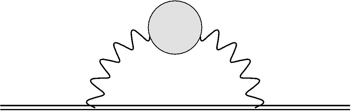
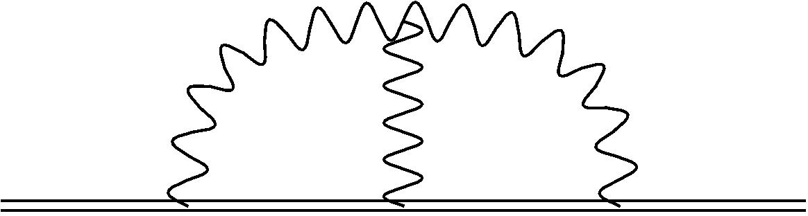
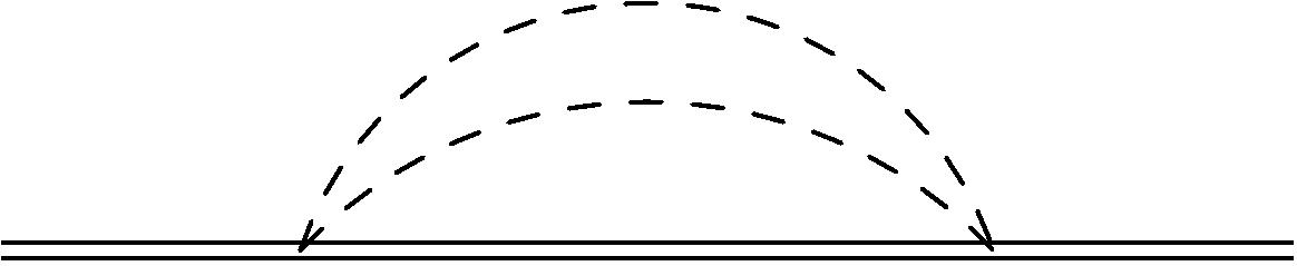
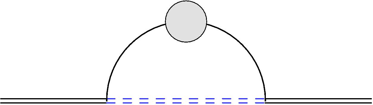
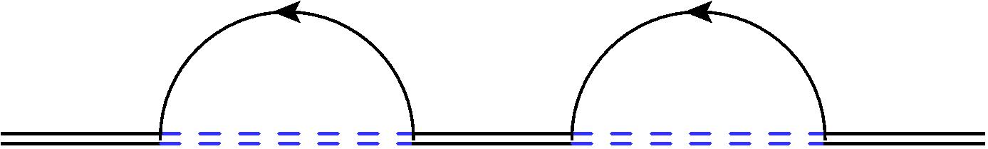
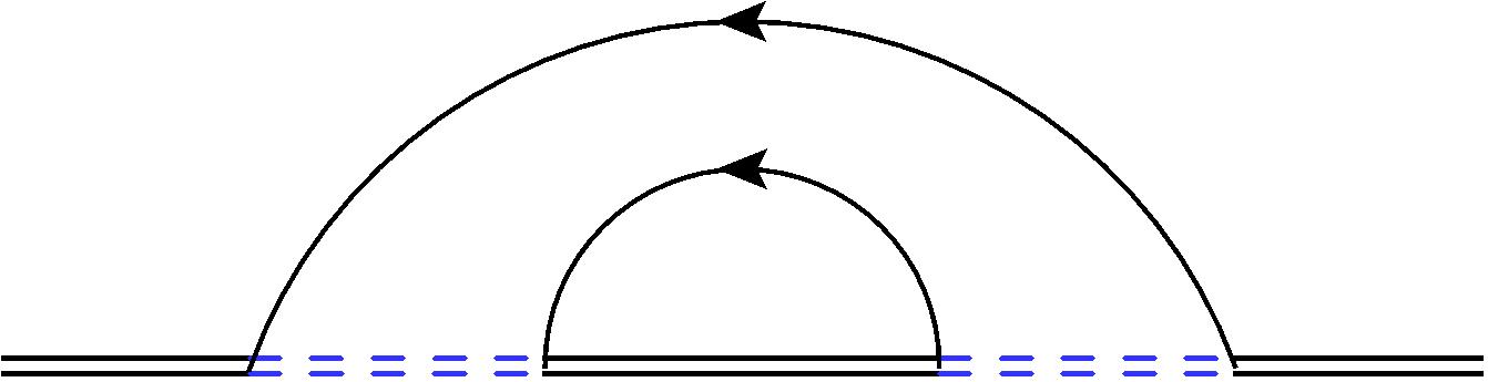
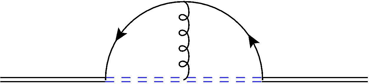
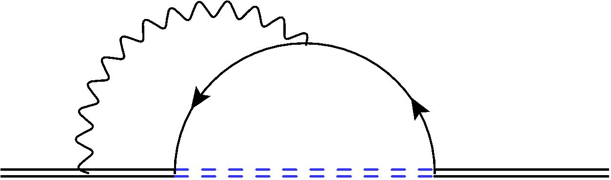
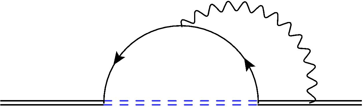
Figure 10: Two-loop corrections to the one-dimensional fermionic propagator $\langle z\bar{z}\rangle$.

Bosonic diagrams

The bosonic diagrams which contribute non-trivially are reported in the first line of figure 10.

Diagram 10 contains the gauge propagator corrected at one loop. Using its explicit expression (A.5), the corresponding contribution to $\langle z\bar{z}\rangle^{(2)}$ reads

$${\rm\ref{subfig:2-loop_bosa}}=-\int_{0}^{2\pi}d\tau_{1}\int_{0}^{\tau_{1}}d\tau_{2}\langle A_{\mu}(\tau_{1})A_{\nu}(\tau_{2})\rangle^{(1)}\dot{x}_{1}^{\mu}\dot{x}^{\nu}_{2}=\frac{g^{4}}{4}N^{2}_{1}N_{2}\,.$$ (4.4)

The result for $\langle\tilde{z}\bar{\tilde{z}}\rangle^{(2)}$ is the same with $N_{1}$ and $N_{2}$ exchanged.

Diagram 10 contains the ABJ(M) pure gauge vertex. Exploiting the results in Bianchi:2013zda ; Bianchi:2013rma for the corresponding integral, this gives

$${\rm{\ref{subfig:2-loop_bosb}}}=-\frac{i}{3g^{2}}\int_{0}^{2\pi}d\tau_{1}\int_{0}^{\tau_{1}} d\tau_{2}\int_{0}^{\tau_{2}}d\tau_{3}\,\epsilon^{\alpha\beta\gamma}\dot{x}_{1}^{\mu}\,\dot{x}_{2}^{\nu}\,\dot{x}_{3}^{\rho}$$ (4.5)

$$\times\langle A_{\mu}(\tau_{1})A_{\nu}(\tau_{2})\rangle\langle A_{\rho}(\tau_{3})A_{\alpha}(x)\rangle\langle A_{\beta}(x)A_{\gamma}(x)\rangle=-\frac{g^{4}}{24}N_{1}^{3}\,.$$

The result for $\langle\tilde{z}\bar{\tilde{z}}\rangle^{(2)}$ is the same with $N_{1}^{3}$ replaced by $N_{2}^{3}$.

Diagram 10 deserves more attention, since it is the only diagram which contributes to the 1/24 BPS operator, but is absent in the more supersymmetric cases. Its contribution to $\langle z\bar{z}\rangle^{(2)}$ is

$${\rm\ref{subfig:2-loop_bosc}}=g^{4}N^{2}_{1}N_{2}\frac{\Gamma^{2}(\frac{1}{2}-\epsilon)}{16\pi^{3-2\epsilon}}\int_{0}^{2\pi}d\tau_{1}\int_{0}^{\tau_{1}}d\tau_{2}\,\operatorname{Tr}\left(M(\tau_{1})M(\tau_{2})\right)\frac{1}{|x_{1}-x_{2}|^{2-4\epsilon}}\,.$$ (4.6)

As long as the trace of two $M$ matrices is $\tau$-independent, this integral is identically zero (see for instance Bianchi:2013rma ). This is what happens in the 1/6 and 1/2 BPS cases. However, in the present case this trace acquires a non-trivial $\tau$-dependence proportional to the loop parameters,

$$\operatorname{Tr}\left(M(\tau_{1})M(\tau_{2})\right)\,\to\,8(\bar{\alpha}^{i}\alpha_{i})(\beta^{j}\bar{\beta}_{j})\cos\tau_{12}\,.$$ (4.7)

This modifies the nature of the integral leading to a non-vanishing result. In fact, the resulting integral is the same as the one-loop correction to the gauge field propagator 10. Exploiting that result, we obtain

$$\begin{split}{\rm\ref{subfig:2-loop_bosc}}&=g^{4}N_{1}N_{2}(N_{1}+N_{2})(\bar{\alpha}^{i}\alpha_{i})(\beta^{j}\bar{\beta}_{j})\frac{\Gamma^{2}(\frac{1}{2}-\epsilon)}{2\pi^{3-2\epsilon}}\int_{0}^{2\pi}d\tau_{1}\int_{0}^{\tau_{1}}d\tau_{2}\,\frac{\cos\tau_{12}}{|x_{12}|^{2-4\epsilon}}\\ &=-\frac{g^{4}}{2}(\bar{\alpha}^{i}\alpha_{i})(\beta^{j}\bar{\beta}_{j})N_{1}N_{2}(N_{1}+N_{2})\,.\end{split}$$ (4.8)

Summarizing, the bosonic contribution to the $1/24$ BPS Wilson loop in (4) is

$${\mathcal{B}}=\frac{g^{4}}{4}N_{1}N_{2}(N_{1}+N_{2})-\frac{g^{4}}{24}\left(N_{1}^{3}+N_{2}^{3}\right)-\frac{g^{4}}{2}(\bar{\alpha}^{i}\alpha_{i})(\beta^{j}\bar{\beta}_{j})N_{1}N_{2}(N_{1}+N_{2})\,.$$ (4.9)

Fermionic diagrams

Fermionic diagrams contributing to the two-point functions are depicted in the second and third lines of figure 10. The first diagram 10 contains the one-loop corrected fermion propagator given in (A.5). Since this is proportional to $(N_{1}-N_{2})$, when in (4) we sum up the contribution of $\langle z(2\pi)\bar{z}(0)\rangle$ with the one from $\langle\tilde{z}(2\pi)\bar{\tilde{z}}(0)\rangle$ obtained by exchanging $N_{1}$ with $N_{2}$, they cancel each other. Therefore, this diagram does not contribute to the Wilson loop VEV.

Moving to the double fermion-exchange diagrams illustrated in figures 10-10, using known integrals from the literature Bianchi:2013zda ; Bianchi:2013rma , we obtain

$$\begin{split}{\rm\ref{subfig:2-loop_fer2a}}+{\rm\ref{subfig:2-loop_fer2b}}&=\frac{1}{24}\int d\tau_{1}d\tau_{2}d\tau_{3}d\tau_{4}\,\langle z(2\pi)\bar{z}(0)\big{(}\bar{z}\bar{f}\tilde{\varphi}\big{)}(\tau_{1})\big{(}\bar{z}\bar{f}\tilde{\varphi}\big{)}(\tau_{2})\\ &\qquad\qquad\times\big{(}\bar{\tilde{\varphi}}fz\big{)}(\tau_{3})\big{(}\bar{\tilde{\varphi}}fz\big{)}(\tau_{4})\rangle+(\tau_{1},\tau_{2},\tau_{3},\tau_{4}\text{ permutations})\\ &=\frac{3g^{4}}{8}N_{1}N_{2}(N_{1}+N_{2})(\bar{\alpha}^{i}\alpha_{i}+\beta^{j}\bar{\beta}_{j})^{2}\end{split}$$ (4.10)

Finally, the three diagrams in the last line of figure 10 correspond to the three different ways of contracting the fields that exit the fermion-vector vertex. Their sum reads

$$\begin{split}&{\rm\ref{subfig:2-loop_fer3a}}+{\rm\ref{subfig:2-loop_fer3b}}+{\rm\ref{subfig:2-loop_fer3c}}\\ &=i\int_{0}^{2\pi}d\tau_{1}\int_{0}^{\tau_{1}}d\tau_{2}\int_{0}^{\tau_{2}}d\tau_{3}\Big{[}\langle\bar{f}(\tau_{1})\hat{A}_{\mu}(\tau_{2})\dot{x}^{\mu}_{2}f(\tau_{3})\rangle\\ &\hskip 156.49014pt\langle\bar{f}(\tau_{1})f(\tau_{2})A_{\mu}(\tau_{3})\dot{x}^{\mu}_{3}\rangle+\langle A_{\mu}(\tau_{1})\dot{x}^{\mu}_{1}\bar{f}(\tau_{2})f(\tau_{3})\rangle\Big{]}\,.\end{split}$$ (4.11)

Inserting the explicit expressions (2.24) for the $f,\bar{f}$ functions, we obtain a linear combination of integrals which are the same ones appearing in the ordinary Wilson loop expansion. Therefore, exploiting known results in the literature Bianchi:2013zda ; Bianchi:2013rma and combining the contributions from $\langle z(2\pi)\bar{z}(0)\rangle$ and $\langle\tilde{z}(2\pi)\bar{\tilde{z}}(0)\rangle$, we eventually obtain

$${\rm\ref{subfig:2-loop_fer3a}}+{\rm\ref{subfig:2-loop_fer3b}}+{\rm\ref{subfig:2-loop_fer3c}}=-\frac{g^{4}}{2}N_{1}N_{2}(N_{1}+N_{2})(\bar{\alpha}^{i}\alpha_{i}-\beta^{j}\bar{\beta}_{j})\,.$$ (4.12)

In conclusion, the total sum of fermionic diagrams reads

$${\mathcal{F}}=\frac{3g^{4}}{8}N_{1}N_{2}(N_{1}+N_{2})(\bar{\alpha}^{i}\alpha_{i}+\beta^{j}\bar{\beta}_{j})^{2}-\frac{g^{4}}{2}N_{1}N_{2}(N_{1}+N_{2})(\bar{\alpha}^{i}\alpha_{i}-\beta^{j}\bar{\beta}_{j})\,.$$ (4.13)

Counterterms

As seen in section 3.3, we also need to include diagrams with vertices coming from the counterterms. In particular, for the $\langle z(2\pi)\bar{z}(0)\rangle$ two-loop correction we obtain the four diagrams in figure 11. For all the other one-dimensional fields we have analogous diagrams and the results extend straightforwardly.

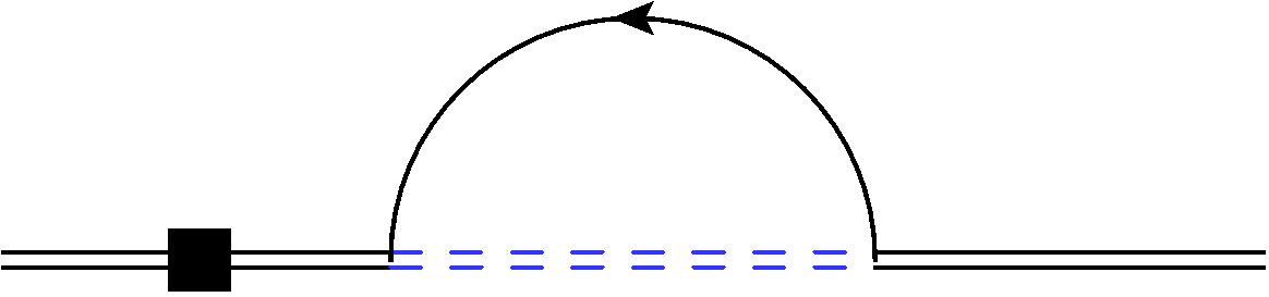
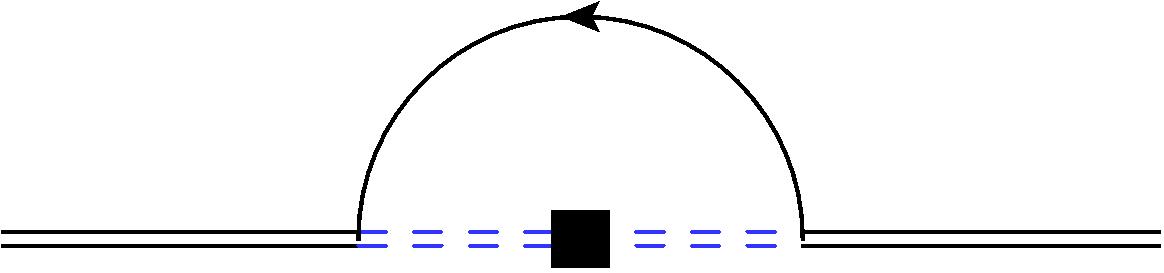
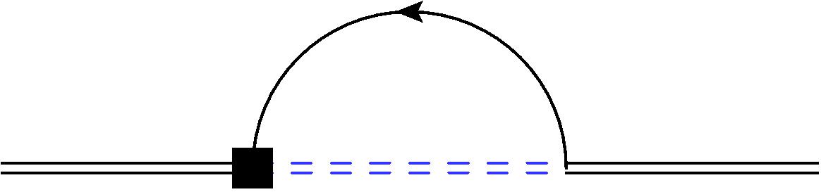
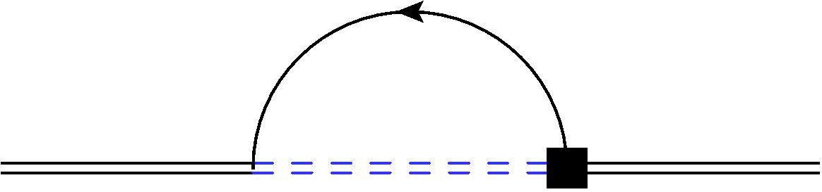
Figure 11: Counterterm contributions to the self-energy of the one-dimensional fermion $z$.

We start from diagram 11, which corresponds to the insertion of a one-loop $\delta_{z}$ counterterm. We obtain

$$\begin{split}{\rm\ref{subfig:diagcounta}}&=\delta_{z}\int d\tau\int d\tau_{1}\int d\tau_{2}\langle z(2\pi)\bar{z}(0)\big{(}\bar{z}\bar{f}\bar{\tilde{\varphi}}\big{)}(\tau_{1})\big{(}\varphi fz\big{)}(\tau_{2})\big{(}\bar{z}\partial_{\tau}z\big{)}(\tau)\rangle+(\tau_{1}\leftrightarrow\tau_{2})\\ &=2\delta_{z}\int_{0}^{2\pi}d\tau_{1}\int_{0}^{\tau_{1}}d\tau_{2}\langle\bar{f}(\tau_{1})f(\tau_{2})\rangle\,,\end{split}$$ (4.14)

where we have used $\partial_{\tau}\theta(\tau-x)=\delta(\tau-x)$. Similarly, from 11 we have

$${\rm\ref{subfig:diagcountb}}=\delta_{\tilde{\varphi}}\int_{0}^{2\pi}d\tau_{1}\int_{0}^{\tau_{1}}d\tau_{2}\langle\bar{f}(\tau_{1})f(\tau_{2})\rangle\,.$$ (4.15)

Diagrams 11 and 11 correspond to insertions of a fermionic counterterm vertex

$${\rm\ref{subfig:diagcountc}}+{\rm\ref{subfig:diagcountd}} =-\frac{1}{2}\int d\tau_{1}\int d\tau_{2}\langle z(2\pi)\bar{z}(0)\big{(}\bar{z}\bar{f}\bar{\tilde{\varphi}}\big{)}(\tau_{1})\big{(}\varphi\,(\delta_{f}f)z\big{)}(\tau_{2})\rangle$$ (4.16)

$$\quad-\frac{1}{2}\int d\tau_{1}\int d\tau_{2}\langle z(2\pi)\bar{z}(0)\big{(}\bar{z}\,(\delta_{\bar{f}}\bar{f})\bar{\tilde{\varphi}}\big{)}(\tau_{1})\big{(}\varphi fz\big{)}(\tau_{2})\rangle+(\tau_{1}\leftrightarrow\tau_{2})$$

$$=-\int_{0}^{2\pi}d\tau_{1}\int_{0}^{\tau_{1}}d\tau_{2}\bigg{(}\langle\bar{f}(\tau_{1})\delta_{f}f(\tau_{2})\rangle+\langle\delta_{\bar{f}}\bar{f}(\tau_{1})f(\tau_{2})\rangle\bigg{)}\,,$$

where we have defined

$$\delta_{f}f=e^{-\frac{i\tau}{2}}\xi\left(\delta_{\bar{\alpha}^{1}}\bar{\alpha}^{1}\psi^{2}-\delta_{\bar{\alpha}^{2}}\bar{\alpha}^{2}\psi^{1}\right)+e^{\frac{i\tau}{2}}\eta(\delta_{\beta^{3}}\beta^{3}\psi^{4}-\delta_{\beta^{4}}\beta^{4}\psi^{3})\,.$$ (4.17)

and similarly for $\delta_{\bar{f}}\bar{f}$.

The same calculation can be reproduced for the $\langle\tilde{z}\bar{\tilde{z}}\rangle$ two-point function. Taking into account that $\delta_{\tilde{\varphi}}=\delta_{\tilde{z}}$ and $\delta_{\varphi}=\delta_{z}$ the total contribution is

$$\left(\langle z(2\pi)\bar{z}(0)\rangle+\langle\tilde{z}(2\pi)\bar{\tilde{z}}(0)\rangle\right)^{\text{ct}}=\left(\delta_{f}+\delta_{\bar{f}}-3\delta_{z}-3\delta_{\tilde{z}}\right)\langle W\rangle^{(1)}\,,$$ (4.18)

where $\langle W\rangle^{(1)}$ is the one-loop contribution to circular Wilson loops (4.3).

According to expansion (4.2), at two loops we have extra finite contributions coming from the product of the one-loop counterterms (set $\delta^{(1)}_{z}\equiv\delta_{z},\delta_{\tilde{z}}$ there) multiplying the one-loop ${\cal O}(\epsilon)$ two-point functions

$$\delta_{z}\langle z(2\pi)\bar{z}(0)\rangle^{(1)}+\delta_{\tilde{z}}\langle\tilde{z}(2\pi)\bar{\tilde{z}}(0)\rangle^{(1)}=\left(\delta_{z}+\delta_{\tilde{z}}\right)\langle W\rangle^{(1)}\,.$$ (4.19)

Therefore, summing (4.18) and (4.19), the final contribution to the Wilson loop VEV from the counterterms is

$${\mathcal{C}}=-g^{4}\frac{N_{1}N_{2}}{4}(N_{1}+N_{2})\left[(\bar{\alpha}^{i}\alpha_{i}+\beta^{j}\bar{\beta}_{j})^{2}-\bar{\alpha}^{i}\alpha_{i}+\beta^{j}\bar{\beta}_{j}\right]\,.$$ (4.20)

4.3 The final result for the Wilson loop VEV

Combining all the previous results, ${\cal B}+{\cal F}+{\cal C}$, the large $N_{1},N_{2}$ expectation value for the parametric circular $1/24$ BPS Wilson loop at two loops reads

$$\langle{\mathcal{W}}_{1/24}(\alpha_{i},\bar{\alpha}^{i},\beta^{j},\bar{\beta}_{j})\rangle=1-\frac{g^{4}}{24}\left[N_{1}^{2}+N_{2}^{2}-4N_{1}N_{2}-3N_{1}N_{2}(\bar{\alpha}^{i}\alpha_{i}-\beta^{j}\bar{\beta}_{j}-1)^{2}\right]+{\mathcal{O}}(g^{6})\,,$$ (4.21)

where we recall that we have defined $g=\sqrt{2\pi/k}$.

By setting $\beta^{j}=\bar{\beta}_{j}=0$ or $\bar{\alpha}^{i}=\alpha_{i}=0$, one recovers two branches of interpolating $1/6$ BPS fermionic Wilson loops, which have the following VEVs

$$\begin{split}\langle{\mathcal{W}}_{1/6}^{\textrm{I}}(\alpha_{i},\bar{\alpha}^{i})\rangle&=1-\frac{g^{4}}{24}\left[N_{1}^{2}+N_{2}^{2}-4N_{1}N_{2}-3N_{1}N_{2}(\bar{\alpha}^{i}\alpha_{i}-1)^{2}\right]+{\mathcal{O}}(g^{6})\,,\\ \langle{\mathcal{W}}_{1/6}^{\textrm{II}}(\beta^{j},\bar{\beta}_{j})\rangle&=1-\frac{g^{4}}{24}\left[N_{1}^{2}+N_{2}^{2}-4N_{1}N_{2}-3N_{1}N_{2}(\beta^{j}\bar{\beta}_{j}+1)^{2}\right]+{\mathcal{O}}(g^{6})\,.\end{split}$$ (4.22)

We recall that, according to the classification in Ouyang:2015iza ; Ouyang:2015bmy , “type I” and “type II” $1/6$ BPS fermionic Wilson loops differ by the preserved $SU(2)\subset SU(4)$ R-symmetry group.

If in particular we choose $\bar{\alpha}^{i}\alpha_{i}=1$ in ${\mathcal{W}}_{1/6}^{\textrm{I}}(\alpha_{i},\bar{\alpha}^{i})$ or $\beta^{j}\bar{\beta}_{j}=-1$ in ${\mathcal{W}}_{1/6}^{\textrm{II}}(\beta^{j},\bar{\beta}_{j})$, we recover the known result for 1/2 BPS operators Bianchi:2013zda ; Bianchi:2013rma ; Griguolo_2013a , at two loops and in the large $N_{1},N_{2}$ limit:

$$\begin{split}\langle{\mathcal{W}}^{\textrm{I}}_{1/2}\rangle=\langle{\mathcal{W}}^{\textrm{II}}_{1/2}\rangle=1-\frac{g^{4}}{24}\left(N_{1}^{2}+N_{2}^{2}-4N_{1}N_{2}\right)+{\mathcal{O}}(g^{6})\,.\end{split}$$ (4.23)

Finally, if we set all the parameters to zero we obtain the two-loop expectation value of the bosonic operator Drukker:2008zx ; Chen:2008bp ; Kluson:2008zrv ; Rey:2008bh

$$\langle{\mathcal{W}}_{1/6}^{\rm bos}\rangle\equiv\left\langle\frac{N_{1}{\cal W}^{\rm bos}+N_{2}\hat{\cal W}^{\rm bos}}{N_{1}+N_{2}}\right\rangle=1-\frac{g^{4}}{24}\left(N_{1}^{2}+N_{2}^{2}-7N_{1}N_{2}\right)+{\mathcal{O}}(g^{6}).$$ (4.24)

where ${\cal W}^{\rm bos},\hat{\cal W}^{\rm bos}$ are the bosonic operators defined in (2.4).

We have evaluated the Wilson loop VEVs exploiting the one-dimensional auxiliary field formulation. Alternatively, one could use the ordinary procedure of expanding $W$ in powers of the superconnection and evaluate correlation functions of ${\cal L}$. We have checked that proceeding in this way, once we replace bare parameters with their renormalized expressions found above, the final result coincides with (4.21). This is a non-trivial check of our procedure.

5 Discussion

5.1 Renormalization Group flows

In section 3.4 we have shown that the introduction of the weakly relevant couplings $\alpha_{i},\bar{\alpha}^{i},\beta^{j},\bar{\beta}_{j}$ triggers a RG flow driven by the eight $\beta$-functions (3.46). Here we study this flow by focusing on the “type I” operators defined above. The study of RG flows involving “type II” Wilson loops will be presented elsewhere CPTT .

In order to give an intuitive visual description of the RG flow we define $\bar{\alpha}^{1}=\alpha_{1}=x$ and $\beta^{3}=\bar{\beta}_{3}=y$ and set the other parameters to zero. The relevant $\beta$-functions are then

$$\begin{split}\beta_{x}(x,y)&=\mu\frac{\partial x}{\partial\mu}=\frac{g^{2}}{4\pi}(N_{1}+N_{2})(x^{2}+y^{2}-1)\,x\,,\\ \beta_{y}(x,y)&=\mu\frac{\partial y}{\partial\mu}=\frac{g^{2}}{4\pi}(N_{1}+N_{2})(x^{2}+y^{2}+1)\,y\,.\end{split}$$ (5.1)

In figure 12 we plot $\beta_{x}(x,y=0)$ and highlight the zeros of the $\beta_{x}$-function.

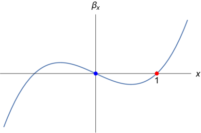
Figure 12: Plot of $\beta_{x}$ when $y=0$. To make contact with figure 13, we have highlighted the fixed points.

In figure 13 we draw the RG flow trajectories in the $(x,y)$ plane, for $x,y$ real and non-negative. For negative $x$ we would obtain an equivalent fixed point. The blue point in figures 12, 13 corresponds to the $x=y=0$ fixed point where the associated operator is the bosonic $1/6$ BPS Wilson loop ${\cal W}_{1/6}^{\rm bos}$ defined in (4.24). This is a UV fixed point where the parameters trigger an outgoing flow. Moving along the horizontal green line in figure 13 we reach an IR fixed point (highlighted in red) corresponding to “type I” fermionic $1/2$ BPS Wilson loop obtained from ${\mathcal{W}}^{\textrm{I}}_{1/6}$ by selecting $\bar{\alpha}^{i}\alpha_{i}=1$.

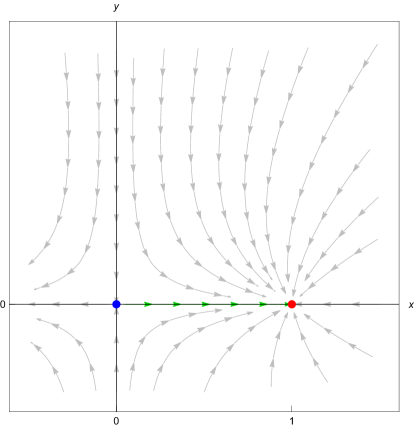
Figure 13: The RG flow in the $(x,y)$ plane. Arrows go from the UV to the IR. Arrows on the $x,y$ axes correspond to $1/6$ BPS flows, while arrows outside the $x,y$ axes correspond to $1/24$ BPS flows. Horizontal green arrows correspond to the RG flow between the bosonic $1/6$ BPS Wilson loop (blue dot) and “type I” fermionic $1/2$ BPS Wilson loop described by $\langle{\mathcal{W}}^{\textrm{I}}_{1/6}(\alpha_{i},\bar{\alpha}^{i})\rangle$ at $\bar{\alpha}^{i}\alpha_{i}=1$ (red dot).

The green line describes an enriched RG flow between UV and IR fixed points, along which supersymmetry is partially preserved. In fact, all the points on the two axes, even those not highlighted in green, correspond to operators which preserve four supercharges.

Similarly, flows along a generic direction in the plane preserve one supercharge, corresponding to the $1/24$ BPS operator, whose VEV is given in (4.21). In this sense, they can still be interpreted as enriched RG flows.

More generally, still setting $y=0$, we relax the condition $\bar{\alpha}^{1}=\alpha_{1}=x$, and consider the flow in the $(\alpha_{1},\bar{\alpha}^{1})$ plane, as presented in figure 14. As expected, the $1/2$ BPS curve $\alpha_{1}\bar{\alpha}^{1}=1$ corresponds to a set of attractive points. This is in agreement with the analysis of figure 13 where the red dot is also attractive and green trajectories connect fixed points.

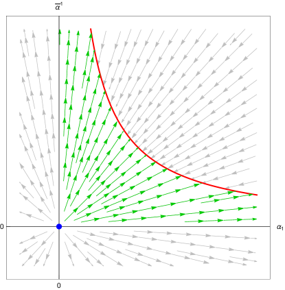
Figure 14: The RG flow in the $(\alpha_{1},\bar{\alpha}^{1})$ plane. Arrows go from the UV to the IR. The red curve corresponds to $\alpha_{1}\bar{\alpha}^{1}=1$ and the blue dot is the bosonic $1/6$ BPS Wilson loop.

5.2 The defect SQFT

Non-local operators like Wilson loops can be used to describe one-dimensional defect quantum field theories (dQFTs). In particular, if the operator preserves the one-dimensional conformal algebra $sl(2,{\mathbb{R}})$, it defines a defect conformal field theory (dCFT). In addition, if the operator is BPS and preserves a sufficient amount of supersymmetry, the corresponding defect is a superconformal field theory (dSCFT).

Focusing on the set of ABJ(M) circular Wilson loops considered in this paper, it is well known that the 1/6 and 1/2 BPS fermionic operators preserve the $su(1,1|1)$ and $su(1,1|3)$ one-dimensional superconformal algebras, respectively. Therefore, they describe superconformal defects. Instead, the new 1/24 BPS operator defined in (2.8)-(2.10) describes a supersymmetric, but not (super)conformal defect, as it preserves only one supercharge and the dependence of the scalar couplings on the contour coordinate breaks conformal invariance.

Regardless of their superconformal or only supersymmetric nature, the dQFTs supported by ABJ(M) fermionic Wilson loops are generated by local operators defined by $U(N_{1}|N_{2})$ supermatrices localized on the Wilson loop. The dQFT is featured by the set of correlation functions of these local operators, inserted on the Wilson loop vacuum. Precisely, the defect $n$-point function of a set of local operators inserted at points $\tau_{1},\ldots,\tau_{n}$ along the circle is defined as

$$\operatorname{\big{\langle}\big{\langle}}\operatorname{Tr}\left(O_{n}O_{n-1}\ldots O_{1}\right)\operatorname{\big{\rangle}\big{\rangle}}\equiv\frac{\left\langle\operatorname{Tr}{\mathcal{P}}\left(e^{-i\int_{\tau_{n}}^{2\pi}d\tau{\mathcal{L}}(\tau)}O_{n}e^{-i\int_{\tau_{n-1}}^{\tau_{n}}d\tau{\mathcal{L}}(\tau)}O_{n-1}\ldots O_{1}e^{-i\int_{0}^{\tau_{1}}d\tau{\mathcal{L}}(\tau)}\right)\right\rangle}{\langle{\cal W}\rangle}\,,$$ (5.2)

where in the right hand side the expectation value is on the ABJ(M) vacuum. The insertion of Wilson links ensures gauge invariance. In the one-dimensional auxiliary field formalism introduced in section 3.1 the defect $n$-point function can be written entirely in terms of ABJ(M) expectation values of products of supermatrices localized on the contour

$$\operatorname{\big{\langle}\big{\langle}}\operatorname{Tr}\left(O_{n}O_{n-1}\ldots O_{1}\right)\operatorname{\big{\rangle}\big{\rangle}}\equiv\frac{1}{2^{n+1}}\frac{\langle\operatorname{Tr}\left(\Psi(2\pi)\bar{\Psi}(\tau_{n})O_{n}\Psi(\tau_{n})\bar{\Psi}(\tau_{n-1})O_{n-1}\ldots O_{1}\Psi(\tau_{1})\bar{\Psi}(0)\right)\rangle}{\langle\operatorname{Tr}\Psi(2\pi)\bar{\Psi}(0)\rangle}\,.$$ (5.3)

In this context, the $(x,y)$ plane depicted in figure 13 has the nice interpretation of describing different defect theories, with fixed points corresponding to theories at their critical point. The blue point is a UV unstable fixed point corresponding to a one-dimensional ${\cal N}=1$ SCFT. The red point represents an interacting IR critical theory where supersymmetry gets enhanced to ${\cal N}=3$.

The Wilson loop RG flows that we have found are interpreted as flows in the space of one-dimensional defects. The two axes describe a continuum of one-dimensional SCFTs. Along these two directions the enriched flow preserves ${\cal N}=1$ superconformal invariance. As soon as we move out of the two axes, superconformal invariance is broken, although one supercharge is still preserved. Nevertheless along all of these flows the system is driven towards the IR fixed point corresponding to ${\mathcal{W}}_{1/2}^{\textrm{I}}$.

It is important to give a closer look at the weakly relevant operators which perturb the system and drive it away from the UV fixed point. To this end, we recall that the UV fixed point corresponds to the bosonic Wilson operator ${\cal W}_{1/6}^{\rm bos}$ obtained by setting all the parameters to zero. Moving along the two green lines in figure 13 amounts to adding a deforming operator as ${\cal L}_{1/6}^{\rm bos}\rightarrow{\cal L}_{1/6}^{\rm bos}+{\cal L}^{\rm def}$. For instance, if we move along the horizontal axis, which amounts to setting $\beta^{j}=\bar{\beta}_{j}=0$, and choose for simplicity $\alpha_{1}=\bar{\alpha}^{1}=0$, we have

$${\cal L}^{\rm def}=\bar{\alpha}^{2}\alpha_{2}\begin{pmatrix}-\frac{4\pi i}{k}C_{2}\bar{C}^{2}&0\\ 0&-\frac{4\pi i}{k}\bar{C}^{2}C_{2}\end{pmatrix}-\bar{\alpha}^{2}\,e^{i\tau/2}\begin{pmatrix}0&\eta\bar{\psi}^{1}\\ 0&0\end{pmatrix}-\alpha_{2}\,e^{-i\tau/2}\begin{pmatrix}0&0\\ \xi\psi_{1}&0\end{pmatrix}\,.$$ (5.4)

We are interested in computing the anomalous dimensions of these operators. This amounts to computing their two-point functions in the bosonic $1/6$ BPS defect.

Focusing on the two fermionic operators, it is easy to see that their integrated two-point function can be expressed as

$$\int_{0}^{2\pi}d\tau_{1}\int_{0}^{\tau_{1}}d\tau_{2}\left[\frac{e^{i\frac{\tau_{12}}{2}}\operatorname{\big{\langle}\big{\langle}}(\eta\bar{\psi}^{1})(\tau_{1})(\xi\psi_{1})(\tau_{2})\operatorname{\big{\rangle}\big{\rangle}}+e^{-i\frac{\tau_{12}}{2}}\operatorname{\big{\langle}\big{\langle}}(\xi\psi_{1})(\tau_{1})(\eta\bar{\psi}^{1})(\tau_{2})\operatorname{\big{\rangle}\big{\rangle}}}{N_{1}+N_{2}}\right]_{\alpha_{2},\bar{\alpha}^{2}=0}=\\ \qquad=-\frac{\partial^{2}}{\partial\alpha_{2}\partial\bar{\alpha}^{2}}\log\langle{\cal W}^{I}_{1/6}(\alpha_{2},\bar{\alpha}^{2})\rangle\Bigg{|}_{\alpha_{2},\bar{\alpha}^{2}=0}\,.$$ (5.5)

If the operators develop an anomalous dimension $\gamma$, the left hand side of this equation formally becomes

$$\begin{split}-\frac{g^{2}}{\pi}\frac{N_{1}N_{2}}{N_{1}+N_{2}}\int_{0}^{2\pi}\!\!\!\!d\tau_{1}\int_{0}^{\tau_{1}}\!\!\!\!d\tau_{2}\,\frac{1}{|4\sin^{2}\frac{\tau_{12}}{2}|^{1+\gamma}}&=-\frac{\sqrt{\pi}g^{2}}{2}\frac{N_{1}N_{2}}{N_{1}+N_{2}}\frac{\Gamma(-\frac{1}{2}-\gamma)}{\Gamma(-\gamma)}\\ &\underset{|\gamma|\ll 1}{\simeq}-g^{2}\pi\frac{N_{1}N_{2}}{N_{1}+N_{2}}\gamma\,.\end{split}$$ (5.6)

On the other hand, the right hand side of (5.5) can be easily evaluated observing that the two-loop result satisfies the following identity

$$\frac{\partial}{\partial\bar{\alpha}^{2}}\log\langle{\cal W}^{I}_{1/6}(\alpha_{2},\bar{\alpha}^{2})\rangle=\kappa\,\beta_{\alpha_{2}}\,,\qquad\text{with }\qquad\kappa=\pi g^{2}\frac{N_{1}N_{2}}{N_{1}+N_{2}}\,.$$ (5.7)

Therefore, comparing the two expressions we finally obtain

$$\gamma=\frac{\partial\beta_{\alpha_{2}}}{\partial\alpha_{2}}\Bigg{|}_{\alpha_{2},\bar{\alpha}^{2}=0}=-\frac{g^{2}}{4\pi}(N_{1}+N_{2})\,.$$ (5.8)

This result can also be checked by explicitly computing the first order correction to the two-point function in (5.5).

We have found that the first contribution to the anomalous dimension of the fermionic fields is negative. With a similar reasoning, one can check that also the bi-scalar operator $C_{2}\bar{C}^{2}$ acquires negative anomalous dimension. This confirms that the deformation (5.4) is a weakly relevant operator.

More generally, we can compute the $\psi_{1},\bar{\psi}^{1}$ anomalous dimension in the ${\cal W}^{I}_{1/6}(\alpha_{2},\bar{\alpha}^{2})$ defect. This amounts to evaluating the derivative of the $\beta$-function without fixing the values of the parameters. We easily find

$$\gamma(\alpha_{2},\bar{\alpha}^{2})=\frac{\partial\beta_{\alpha_{2}}}{\partial\alpha_{2}}=\frac{g^{2}}{4\pi}(N_{1}+N_{2})(2\bar{\alpha}^{2}\alpha_{2}-1)\,.$$ (5.9)

This interpolates between the dimension of the weakly relevant operator in the UV and its dimension in the IR.

5.3 A g-theorem

Focusing on $1/6$ BPS flow along the green line we now prove the validity of a g-theorem. In order to keep the discussion simpler we again set $\alpha_{1}=\bar{\alpha}^{1}=x$ and $\beta^{3}=\bar{\beta}_{3}=y$ with other parameters set to zero.

Referring to the $\beta$-function as written in (5.1), in the $x\in[0,1]$ region we can write

$$\frac{\partial}{\partial x}\log\langle{\mathcal{W}}^{\textrm{I}}_{1/6}(x)\rangle=2\kappa\,\beta_{x}\Big{|}_{y=0}\,.$$ (5.10)

where $\kappa$ has been defined in (5.7). First of all, this implies that the blue and the red conformal fixed points in figure 13 are extrema of $\langle{\mathcal{W}}_{1/24}(\alpha_{i},\bar{\alpha}^{i},\beta^{j},\bar{\beta}_{j})\rangle$. Moreover, it is easy to show that the (red) $1/2$ BPS point is a minimum while the (blue) bosonic $1/6$ BPS point is a maximum. Therefore, comparing the two fixed points connected by the horizontal green line in figure 13, we can write

$$\log\langle{\mathcal{W}}_{1/6}^{\textrm{bos}}\rangle\equiv\log\langle{\mathcal{W}}_{1/6}^{\textrm{I}}(x=0)\rangle>\log\langle{\mathcal{W}}_{1/6}^{\textrm{I}}(x=1)\rangle\equiv\log\langle{\mathcal{W}}^{\textrm{I}}_{1/2}\rangle\,.$$ (5.11)

This result can be interpreted as a g-theorem Cuomo:2021rkm for the one-dimensional defect. In fact, defining the interpolating functions $g^{\textrm{I}}=\langle{\mathcal{W}}^{\textrm{I}}_{1/6}\rangle$, we find $g^{\textrm{I}}_{UV}>g^{\textrm{I}}_{IR}$. Recalling that $\log\langle{\mathcal{W}}\rangle$ is nothing but the partition function of the one-dimensional defect, monotonicity is consistent with the decreasing of degrees of freedom from the UV to the IR fixed point. Our result is in line with what has been already found in ${\mathcal{N}}=4$ super Yang-Mills Beccaria:2017rbe ; Beccaria:2018ocq , although in a different setup, as it consists of BPS flows.

5.4 Comparison with the localization result

It is well known that in supersymmetric theories defined on compact manifolds BPS Wilson loops can be computed using supersymmetric localization Pestun_2012 . This provides a representation of the path integral evaluating the Wilson loop VEV as a matrix integral.

For the ABJ(M) theory on $S^{3}$ localization allows to exactly compute the VEV of the bosonic Wilson loops in (2.4) as the expectation values

$$\langle{\mathcal{W}}^{\rm bos}\rangle_{1}=\left\langle\frac{1}{N_{1}}\sum_{i=1}^{N_{1}}e^{2\pi\lambda_{i}}\right\rangle_{{}_{\mathcal{Z}}}\,,\qquad\langle\hat{\cal W}^{\rm bos}\rangle_{1}=\left\langle\frac{1}{N_{2}}\sum_{i=1}^{N_{2}}e^{2\pi\hat{\lambda}_{i}}\right\rangle_{{}_{\mathcal{Z}}}\,,$$ (5.12)

where the average is evaluated and normalized using the following non-Gaussian matrix model Kapustin:2009kz

$${\mathcal{Z}}=\int\prod_{i=1}^{N_{1}}d\lambda_{i}e^{i\pi k\lambda^{2}_{i}}\prod^{N_{2}}_{j=1}d\hat{\lambda}_{j}e^{-i\pi k\hat{\lambda}^{2}_{j}}\frac{\prod_{i<j}^{N_{1}}\sinh^{2}(\pi(\lambda_{i}-\lambda_{j}))\prod_{i<j}^{N_{2}}\sinh^{2}(\pi(\hat{\lambda}_{i}-\hat{\lambda}_{j}))}{\prod_{i=1}^{N_{1}}\prod_{j=1}^{N_{2}}\cosh^{2}(\pi(\lambda_{i}-\hat{\lambda}_{j}))}\,.$$ (5.13)

Here the integrations are on two complete sets of eigenvalues $\{\lambda_{i}\}$, $\{\hat{\lambda}_{j}\}$ of the Cartan subalgebras of $U(N_{1})$ and $U(N_{2})$, respectively. The “1” subscript in (5.12) indicates that the matrix model computes the expectation values at framing $f=1$ Kapustin:2009kz .

The main observation is that the prescription (5.12) automatically provides exact results for the whole class of BPS Wilson loops that we have considered in this paper. This stems from the fact that, classically, the 1/24 BPS, the 1/6 BPS fermionic and the 1/2 BPS Wilson loops are all cohomologically equivalent to the linear combination ${\cal W}_{1/6}^{\rm bos}$ defined in (4.24). In other words, they differ from ${\cal W}_{1/6}^{\rm bos}$ by a ${\cal Q}$-exact term, where ${\cal Q}$ is one of the supercharges preserved by all the operators in the game. Therefore, if cohomological equivalence is preserved at the quantum level, one can in principle use this ${\cal Q}$ to localize the path integral for the Wilson loop VEV. As a consequence, the following identities hold

$$\langle{\mathcal{W}}_{1/24}(\alpha_{i},\bar{\alpha}^{i},\beta^{j},\bar{\beta}_{j})\rangle_{1}=\langle{\mathcal{W}}_{1/6}^{\textrm{I}}(\alpha_{i},\bar{\alpha}^{i})\rangle_{1}=\langle{\mathcal{W}}_{1/6}^{\textrm{II}}(\beta^{j},\bar{\beta}_{j})\rangle_{1}=\langle{\mathcal{W}}_{1/2}^{\textrm{I,II}}\rangle_{1}=\langle{\cal W}_{1/6}^{\rm bos}\rangle_{1}\,.$$ (5.14)

At framing one, all the VEVs must equal $\langle{\cal W}_{1/6}^{\rm bos}\rangle_{1}=(N_{1}\langle{\cal W}^{\rm bos}\rangle+N_{2}\langle\hat{\cal W}^{\rm bos}\rangle)/(N_{1}+N_{2})$, which can be easily evaluated from (5.12). At weak coupling, this quantity is known both from the matrix model expansion Kapustin:2009kz and from perturbation theory Mauri_2018 . Up to two loops it reads

$$\langle{\cal W}_{1/6}^{\rm bos}\rangle_{1}=1+\frac{i\pi(N_{1}-N_{2})}{k}-\frac{\pi^{2}}{6k^{2}}\left[4(N_{1}^{2}+N_{2}^{2})-10N_{1}N_{2}-1\right]\,.$$ (5.15)

Therefore, as a consequence of identities (5.14), at $f=1$ the VEVs loose any dependence on the alpha and beta parameters. In other words, all the points of the plot in figure 13 correspond to the same quantum operator. It is then interesting to understand how the parameter dependence arises when the expectation values are evaluated at $f\neq 1$, in particular at framing zero.

For 1/6 BPS bosonic and 1/2 BPS fermionic Wilson loops, a relation between their expectation values at framing zero computed perturbatively and the ones at framing one coming from the matrix model has been found Drukker:2009hy ; Bianchi_2016 . Up to two loops, these read

$$\langle{\cal W}^{\rm bos}\rangle_{1}=e^{\frac{i\pi N_{1}}{k}}\langle{\cal W}^{\rm bos}\rangle_{0}\,,\quad\langle\hat{\cal W}^{\rm bos}\rangle_{1}=e^{-\frac{i\pi N_{2}}{k}}\langle\hat{\cal W}^{\rm bos}\rangle_{0}\,,\quad\langle{\cal W}^{\textrm{I,II}}_{1/2}\rangle_{1}=e^{\frac{i\pi(N_{1}-N_{2})}{k}}\langle{\cal W}_{1/2}\rangle_{0}\,.$$ (5.16)

They can be generalized to generic (also non-integer) framing $f$ in a rather simple way, see the discussion in Bianchi:2014laa .

Since the interpolating operators under investigation have a non-trivial parametric dependence at framing zero, but loose this dependence at framing one, we expect the parameter dependence to be carried by “phase” factors, in analogy with (5.16). Perturbative analysis reveals that up to two loops and in the large $N_{1},N_{2}$ limit, the matrix model results (5.14)-(5.15) are related to the perturbative ones in section 4.3 as follows. For the fermionic 1/6 BPS operators we are led to the following identities

$$\begin{split}&\langle{\cal W}_{1/6}^{\textrm{I}}(\bar{\alpha}^{i},\alpha_{i})\rangle_{1}=\frac{N_{1}e^{\frac{i\pi}{k}(N_{1}-\bar{\alpha}^{i}\alpha_{i}N_{2})}+N_{2}\,e^{\frac{i\pi}{k}(\bar{\alpha}^{i}\alpha_{i}N_{1}-N_{2})}}{N_{1}+N_{2}}\langle{\cal W}_{1/6}^{\textrm{I}}(\bar{\alpha}^{i},\alpha_{i})\rangle_{0}\,,\\ &\langle{\cal W}_{1/6}^{\textrm{II}}(\beta^{j},\bar{\beta}_{j})\rangle_{1}=\frac{N_{1}e^{\frac{i\pi}{k}(N_{1}+\beta^{j}\bar{\beta}_{j}N_{2})}+N_{2}\,e^{\frac{i\pi}{k}(-\beta^{j}\bar{\beta}_{j}N_{1}-N_{2})}}{N_{1}+N_{2}}\langle{\cal W}_{1/6}^{\textrm{II}}(\beta^{j},\bar{\beta}_{j})\rangle_{0}\,,\end{split}$$ (5.17)

whereas for the more general $1/24$ BPS operator the relation it reads

$$\langle{\cal W}_{1/24}\rangle_{1}=\frac{N_{1}e^{\frac{i\pi}{k}(N_{1}-(\bar{\alpha}^{i}\alpha_{i}-\beta^{j}\bar{\beta}_{j})N_{2})}+N_{2}\,e^{\frac{i\pi}{k}((\bar{\alpha}^{i}\alpha_{i}-\beta^{j}\bar{\beta}_{j})N_{1}-N_{2})}}{N_{1}+N_{2}}\langle{\cal W}_{1/24}\rangle_{0}\,.$$ (5.18)

In the ABJM limit, $N_{1}=N_{2}$, it boils down to

$$\langle{\cal W}_{1/24}(\bar{\alpha}^{i},\alpha_{i},\beta^{j},\bar{\beta}_{j})\rangle_{1}=\cos\left(\tfrac{\pi N}{k}(1-\bar{\alpha}^{i}\alpha_{i}+\beta^{j}\bar{\beta}_{j})\right)\langle{\cal W}_{1/24}(\bar{\alpha}^{i},\alpha_{i},\beta^{j},\bar{\beta}_{j})\rangle_{0}\,.$$ (5.19)

Similar relations come from (LABEL:eqn:MMrelation2) for $N_{1}=N_{2}$.

We note that the exponentials carrying the parameter dependence are no longer pure phases as in (5.16), since the parameters can be generically complex and the barred parameters are not the complex conjugates. However, for the special values $\bar{\alpha}^{i}\alpha_{i}=1$ and $\beta^{j}\bar{\beta}_{j}=0$ they reduce to the last phase in (5.16).

These identities have been empirically inferred from the two-loop results and are not expected to be true in general. In fact, the parametric exponents are likely to be corrected at higher orders, as already happens at three loops for the ${\cal W}^{\rm bos},\hat{\cal W}^{\rm bos}$ phases Bianchi:2016yzj .

We close this section with a technical observation on the integrals in the two schemes, framing or dimensional regularization ($f=0$). The parameter independence of the framing-one results indicates that a genuine perturbative calculation done at $f=1$ should sensibly differ from our present calculation done using dimensional regularization. In particular, new non-vanishing contributions should arise to compensate the parameter dependence carried by diagrams that are framing independent. For instance, let us focus on the contributions proportional to $\bar{\alpha}^{i}\alpha_{i}\beta^{j}\bar{\beta}_{j}$. At two loops and framing zero, they come from the scalar diagram 10 and the two fermion ones, 10 and 10. As shown in Mauri_2018 , the scalar integral is framing independent, thus its dependence on the parameters should survive also at framing one. On the other hand, it has been argued in Bianchi_2016 that at $f=1$ the fermionic diagrams should be identically vanishing. Therefore, at framing one some new parameter dependent contribution should arise, which eventually cancels the scalar diagram. A proof of this statement would require performing a genuine two-loop calculation at framing one, though this might be obstructed by the difficulty of computing fermionic diagrams at non-trivial framing.

5.5 Outlook

There are several natural directions in which these investigations could be extended.

As stressed repeatedly, the flows considered in this paper are BPS, with at least one supercharge preserved at all points of the flow. It would of course be interesting to introduce a $\zeta$-parameter in the 1/24 BPS Wilson loop, to interpolate to a fully non-supersymmetric limit, like it has been done in Polchinski_2011 for the 1/2 BPS circular Wilson loop of ${\mathcal{N}}=4$ super Yang-Mills in four dimensions. This could be achieved by rescaling the overall couplings to the scalars and the fermions in (2.26) and would make the RG flow space even richer, opening up a new direction corresponding to the renormalization of the new parameter. We plan to address this in a future investigation.

As usual, there is always the question of the holographic dual description in terms of minimal surfaces in M-theory or type IIA superstring theory. The 1/24 BPS Wilson loop considered in this paper should be described by mixed boundary conditions in $AdS_{2}$, generalizing what has been done in Correa:2019rdk ; Garay:2022szq for deformations of the 1/6 BPS bosonic operator defined on a straight line. For instance, it would interesting to understand whether the set of boundary conditions that do not preserve conformal invariance – the reason why they were not further discussed in Correa:2019rdk ; Garay:2022szq – may play a role in this context.

We should stress that the generalization of this approach to the present case would require to first adapt it to the circular case, where a conformal anomaly gross makes operators, which are cohomologically equivalent at the classical level, no longer equivalent at the quantum level. In particular, as we have discussed, this causes a non-trivial dependence of the VEVs on the deformations. Therefore, in this case the mixing of Neumann and Dirichlet boundary conditions should entail a non-trivial parametric dependence in the interpolating string solutions. More generally, the question of what is, if any, the holographic counterpart of framing is quite important.

Finally, it is interesting to repeat this analysis for the 1/12 BPS latitude Wilson loop of section 2.2. This is going to be addressed in CPTT . In that case the one-dimensional effective field theory on the Wilson loop is modified by the presence of non-trivial shifts in the superconnection ${\mathcal{L}}^{\theta}$, which result in mass terms for the one-dimensional fields.

Appendix A Conventions and Feynman rules

We follow the conventions in Bianchi:2014laa . We work in three-dimensional Euclidean space with coordinates $x^{\mu}=(x^{0},x^{1},x^{2})$. The three-dimensional gamma matrices are defined as

$$(\gamma^{\mu})^{\ \beta}_{\alpha}=(-\sigma^{3},\sigma^{1},\sigma^{2})_{\alpha}^{\ \beta}\,,$$ (A.1)

with $(\sigma^{i})^{\ \beta}_{\alpha}$ ($\alpha,\beta=1,2$) being the Pauli matrices, such that $\gamma^{\mu}\gamma^{\nu}=\delta^{\mu\nu}+i\epsilon^{\mu\nu\rho}\gamma_{\rho}$, where $\epsilon^{123}=\epsilon_{123}=1$ is totally antisymmetric. Spinorial indices are lowered and raised as $(\gamma^{\mu})^{\alpha}_{\ \beta}=\epsilon^{\alpha\gamma}(\gamma^{\mu})^{\ \delta}_{\gamma}\epsilon_{\beta\delta}$, with $\epsilon_{12}=-\epsilon^{12}=1$. The Euclidean action of $U(N_{1})_{k}\times U(N_{2})_{-k}$ ABJ(M) theory is

$$\begin{split}S_{\textrm{ABJ(M)}}=&\frac{k}{4\pi}\int d^{3}x\,\epsilon^{\mu\nu\rho}\Big{\{}-i\text{Tr}\left(A_{\mu}\partial_{\nu}A_{\rho}+\frac{2i}{3}A_{\mu}A_{\nu}A_{\rho}\right)+i\text{Tr}\left(\hat{A}_{\mu}\partial_{\nu}\hat{A}_{\rho}+\frac{2i}{3}\hat{A}_{\mu}\hat{A}_{\nu}\hat{A}_{\rho}\right)\\ &+\text{Tr}\left[\frac{1}{\xi}(\partial_{\mu}A^{\mu})^{2}-\frac{1}{\xi}(\partial_{\mu}\hat{A}^{\mu})^{2}+\partial_{\mu}\bar{c}D^{\mu}c-\partial_{\mu}\bar{\hat{c}}D^{\mu}\hat{c}\right]\Big{\}}\\ &+\int d^{3}x\text{Tr}\left[D_{\mu}C_{I}D^{\mu}\bar{C}^{I}+i\bar{\psi}^{I}\gamma^{\mu}D_{\mu}\psi_{I}\right]\\ &\begin{split}-\frac{2\pi i}{k}\int d^{3}x\text{Tr}\Big{[}&\bar{C}^{I}C_{I}\psi_{J}\bar{\psi}^{J}-C_{I}\bar{C}^{I}\bar{\psi}^{J}\psi_{J}+2C_{I}\bar{C}^{J}\bar{\psi}^{I}\psi_{J}\\ &-2\bar{C}^{I}C_{J}\psi_{I}\bar{\psi}^{J}-\epsilon_{IJKL}\bar{C}^{I}\bar{\psi}^{J}\bar{C}^{K}\bar{\psi}^{L}+\epsilon^{IJKL}C_{I}\psi_{J}C_{K}\psi_{L}\Big{]}+S^{\text{bos}}_{\text{int}}\,,\end{split}\end{split}$$ (A.2)

with covariant derivatives defined as

$$\begin{split}&D_{\mu}C_{I}=\partial_{\mu}C_{I}+iA_{\mu}C_{I}-iC_{I}\hat{A}_{\mu}\,,\qquad D_{\mu}\bar{C}^{I}=\partial_{\mu}\bar{C}^{I}-i\bar{C}^{I}A_{\mu}+i\hat{A}_{\mu}\bar{C}^{I}\,,\\ &D_{\mu}\bar{\psi}^{I}=\partial_{\mu}\bar{\psi}^{I}+iA_{\mu}\bar{\psi}^{I}-i\bar{\psi}^{I}\hat{A}_{\mu}\,,\qquad D_{\mu}\psi_{I}=\partial_{\mu}\psi_{I}-i\psi_{I}A_{\mu}+i\hat{A}_{\mu}\psi_{I}\,.\end{split}$$ (A.3)

We work in Landau gauge for vector fields and in dimensional regularization with $d=3-2\epsilon$. The tree-level propagators are (with $g=\sqrt{2\pi/k}$)

$$\begin{split}\langle(A_{\mu})_{p}^{\ q}(x)(A_{\nu})_{r}^{\ s}(y)\rangle^{(0)}&=\delta_{p}^{s}\delta_{r}^{q}\,ig^{2}\,\frac{\Gamma(\frac{3}{2}-\epsilon)}{2\pi^{\frac{3}{2}-\epsilon}}\frac{\epsilon_{\mu\nu\rho}(x-y)^{\rho}}{|x-y|^{3-2\epsilon}},\\ \langle(\hat{A}_{\mu})_{\hat{p}}^{\ \hat{q}}(x)(\hat{A}_{\nu})_{\hat{r}}^{\ \hat{s}}(y)\rangle^{(0)}&=-\delta_{\hat{p}}^{\hat{s}}\delta_{\hat{r}}^{\hat{q}}\,ig^{2}\,\frac{\Gamma(\frac{3}{2}-\epsilon)}{2\pi^{\frac{3}{2}-\epsilon}}\frac{\epsilon_{\mu\nu\rho}(x-y)^{\rho}}{|x-y|^{3-2\epsilon}},\\ \langle(\psi_{I}^{\alpha})_{\hat{i}}^{j}(x)(\bar{\psi}_{\beta}^{J})_{k}^{\hat{l}}(y)\rangle^{(0)}&=-i\delta_{I}^{J}\delta_{i}^{\hat{l}}\delta_{k}^{j}\frac{\Gamma(\frac{3}{2}-\epsilon)}{2\pi^{\frac{3}{2}-\epsilon}}\frac{(\gamma_{\mu})^{\alpha}_{\ \beta}(x-y)^{\mu}}{|x-y|^{3-2\epsilon}}\\ &=i\delta_{I}^{J}\delta_{i}^{\hat{l}}\delta_{k}^{j}(\gamma_{\mu})^{\alpha}_{\ \beta}\partial_{\mu}\left(\frac{\Gamma(\frac{1}{2}-\epsilon)}{4\pi^{\frac{3}{2}-\epsilon}}\frac{1}{|x-y|^{1-2\epsilon}}\right),\\ \langle(C_{I})_{i}^{\hat{j}}(x)(\bar{C}^{J})_{\hat{k}}^{l}(y)\rangle^{(0)}&=\delta_{I}^{J}\delta_{i}^{l}\delta_{\hat{k}}^{\hat{j}}\frac{\Gamma(\frac{1}{2}-\epsilon)}{4\pi^{\frac{3}{2}-\epsilon}}\frac{1}{|x-y|^{1-2\epsilon}},\end{split}$$ (A.4)

while the one-loop propagators are

$$\begin{split}\langle(A_{\mu})_{p}^{\ q}(x)(A_{\nu})_{r}^{s}(y)\rangle^{(1)}&=\delta_{p}^{s}\delta_{r}^{q}\left(\frac{2\pi}{k}\right)^{2}N_{1}\frac{\Gamma^{2}(\frac{1}{2}-\epsilon)}{4\pi^{3-2\epsilon}}\left[\frac{\delta_{\mu\nu}}{|x-y|^{2-4\epsilon}}-\partial_{\mu}\partial_{\nu}\frac{|x-y|^{2\epsilon}}{4\epsilon(1+2\epsilon)}\right],\\ \langle(\hat{A}_{\mu})_{\hat{p}}^{\ \hat{q}}(x)(\hat{A}_{\nu})_{\hat{r}}^{\hat{s}}(y)\rangle^{(1)}&=\delta_{\hat{p}}^{\hat{s}}\delta_{\hat{r}}^{\hat{q}}\left(\frac{2\pi}{k}\right)^{2}N_{2}\frac{\Gamma^{2}(\frac{1}{2}-\epsilon)}{4\pi^{3-2\epsilon}}\left[\frac{\delta_{\mu\nu}}{|x-y|^{2-4\epsilon}}-\partial_{\mu}\partial_{\nu}\frac{|x-y|^{2\epsilon}}{4\epsilon(1+2\epsilon)}\right],\\ \langle(\psi_{I}^{\alpha})_{\hat{i}}^{j}(x)(\bar{\psi}^{J}_{\beta})_{k}^{\hat{l}}(y)\rangle^{(1)}&=i\delta_{I}^{J}\delta_{\hat{i}}^{\hat{l}}\delta_{\hat{k}}^{\hat{j}}\delta^{\alpha}_{\beta}\left(\frac{2\pi}{k}\right)(N_{1}-N_{2})\frac{\Gamma^{2}(\frac{1}{2}-\epsilon)}{16\pi^{3-2\epsilon}}\frac{1}{|x-y|^{2-4\epsilon}}.\end{split}$$ (A.5)

The latin indices are color indices. For instance, $(A_{\mu})_{p}^{\ q}\equiv A_{\mu}^{a}(T^{a})_{p}^{\ q}$ where $T^{a}$ are $U(N_{1})$ generators in fundamental representation.

Appendix B The auxiliary field method for fermionic Wilson loops

In this section we prove that the ABJ(M) Wilson loop VEV

$$\langle W\rangle=\langle\operatorname{Tr}{\mathcal{P}}e^{-i\int d\tau{\mathcal{L}}}\rangle\,,$$ (B.1)

can be written as the two-point function of the one-dimensional field supermatrix, i.e.

$$\langle W\rangle=\frac{1}{2}\langle\operatorname{Tr}\Psi_{0}\bar{\Psi}_{0}\rangle_{1D}\,,$$ (B.2)

where the one-dimensional fields on the r.h.s. of this equation are the bare ones. In order to simplify the notation, in what follows we will neglect the subscript 0 under the assumption that all the fields have to be meant as bare fields.

We start by defining

$${\mathcal{Z}}[\eta,\bar{\eta}]=\int D\Psi D\bar{\Psi}e^{-\int d\tau\operatorname{Tr}(\bar{\Psi}D_{\tau}\Psi-\bar{\Psi}\eta-\bar{\eta}\Psi)}\,,$$ (B.3)

where ${\mathcal{D}}_{\tau}=\partial_{\tau}+i{\mathcal{L}}$ and

$$\eta=\begin{pmatrix}\chi&\phi\\ \tilde{\phi}&\tilde{\chi}\end{pmatrix}\,,\qquad\qquad\bar{\eta}=\begin{pmatrix}\bar{\chi}&\bar{\tilde{\phi}}\\ \bar{\phi}&\bar{\tilde{\chi}}\end{pmatrix}$$ (B.4)

are odd supermatrices with $\chi$ ($\tilde{\chi}$) and $\phi$ ($\tilde{\phi}$) one-dimensional fermion and scalar fields in the fundamental representation of $U(N_{1})$ ($U(N_{2})$). The one-dimensional fields two-point function can be written as

$$\langle\Psi\bar{\Psi}\rangle_{1D}=\frac{\delta^{2}\log{\mathcal{Z}}[\eta,\bar{\eta}]}{\delta^{L}\bar{\eta}\,\delta^{R}\eta}\Big{|}_{\eta=\bar{\eta}=0}$$ (B.5)

where $\delta^{L}\bar{\eta}$ and $\delta^{R}\eta$ are the left and right derivative respectively, defined as

$$\frac{\delta}{\delta^{L}\bar{\eta}}=\begin{pmatrix}\frac{\delta}{\delta{\bar{\chi}}}&\frac{\delta}{\delta\bar{\phi}}\\ \frac{\delta}{\delta\bar{\tilde{\phi}}}&\frac{\delta}{\delta\bar{\tilde{\chi}}}\end{pmatrix}\,,\qquad\frac{\delta}{\delta^{R}\eta}=\begin{pmatrix}\frac{\delta}{\delta{\chi}}&\frac{\delta}{\delta\tilde{\phi}}\\ \frac{\delta}{\delta\phi}&\frac{\delta}{\delta\tilde{\chi}}\end{pmatrix}\,,$$ (B.6)

such that $\frac{\delta(\theta_{1}\theta_{2})}{\delta^{R}\theta_{2}}=\theta_{1}$, where $\theta_{1},\theta_{2}$ are Grassmann numbers.

Assuming that a consistent definition of integration over supermatrices exists, and that it leads to a well-defined and non-vanishing results for Gaussian integrals, we can solve the path integral in (B.3) with the standard technique of completing the square at the exponent. In particular, we find

$${\mathcal{Z}}[\eta,\bar{\eta}]\propto\exp\int d\tau\,\bar{\eta}D_{\tau}^{-1}\eta\,,$$ (B.7)

where the overall coefficient associated to the result of the supermatrix Gaussian integration is irrelevant, since the two-point function is defined as the derivative of the logarithm of ${\mathcal{Z}}$.

Now, taking the double derivative of (B.7), one can easily check that

$$\frac{\delta^{2}\log{\mathcal{Z}}[\eta,\bar{\eta}]}{\delta^{L}\bar{\eta}\,\delta^{R}\eta}\Big{|}_{\eta=\bar{\eta}=0}=2D_{\tau}^{-1}\,.$$ (B.8)

On the other hand, the following identity holds Arefeva:1980zd ; CRAIGIE1981204 ; Dorn:1986dt

$$D_{\tau}^{-1}=\left(\partial_{\tau}+i{\mathcal{L}}\right)^{-1}=\theta(\tau){\mathcal{P}}e^{-i\int_{0}^{\tau}d\tau^{\prime}{\mathcal{L}}(\tau^{\prime})}\,.$$ (B.9)

In conclusion, combining (B.5) with (B.8) and inserting (B.9), we find

$$\frac{1}{2}\langle\Psi(\tau)\bar{\Psi}(0)\rangle_{1D}=\theta(\tau){\mathcal{P}}e^{-i\int_{0}^{\tau}d\tau^{\prime}{\mathcal{L}}(\tau^{\prime})}\,.$$ (B.10)

Finally, taking the trace and the ABJ(M) expectation value we reproduce (B.1).

Appendix C Perturbative computations

C.1 Gauge-fermion vertex corrections

Here we provide details on the evaluations of the gauge vertex corrections.

We start from diagram in figure 7 that corresponds to the following integral

$$\Gamma^{\rm\ref{subfig:gauge1b}}_{\text{gauge}}=\frac{1}{18g^{2}}\int d\tau_{1}\int d\tau_{2}\int d^{d}x\,\langle\left(\bar{z}_{1}A_{\mu}(\tau_{1})\dot{x}_{1}^{\mu}z_{1}\right)\left(\bar{z}_{2}A_{\nu}(\tau_{2})\dot{x}_{2}^{\nu}z_{2}\right)\left(\epsilon^{\rho\sigma\tau}A_{\rho}A_{\sigma}A_{\tau}\right)(x)\rangle.$$ (C.1)

It is easy to see that this contribution is vanishing due to the antisymmetry of the $\epsilon$ tensor. In fact, to begin with, we perform the contractions using the one-dimensional and gauge fields propagators. We obtain

$$\Gamma^{\rm\ref{subfig:gauge1b}}_{\text{gauge}}\sim\int d\tau_{1}\int^{\tau_{1}}d\tau_{2}\int d^{d}x\bar{z}_{1}\dot{x}^{\mu}_{1}\dot{x}^{\nu}_{2}z_{2}A_{\rho}\,\epsilon^{\rho\sigma\tau}\epsilon_{\mu\sigma\omega}\epsilon_{\nu\tau\eta}\,\frac{(x_{1}-x)^{\omega}(x_{2}-x)^{\eta}}{|x_{1}-x|^{d}|x_{2}-x|^{d}}.$$ (C.2)

Then, we take the $\tau_{2}\to\tau_{1}$ limit focusing only on the potentially divergent terms. The numerator of (C.2) turns out to be proportional to

$$\epsilon^{\rho\sigma\tau}\epsilon_{\mu\sigma\omega}\epsilon_{\nu\tau\eta}\,\dot{x}^{\mu}_{1}\dot{x}^{\nu}_{1}(x_{1}-x)^{\omega}\left[(x_{1}-x)^{\eta}+(\tau_{2}-\tau_{1})\dot{x}^{\eta}_{1}\right].$$ (C.3)

By using the following relation

$$\epsilon^{\rho\sigma\tau}\epsilon_{\mu\sigma\omega}\epsilon_{\nu\tau\eta}=(\delta^{\rho}_{\mu}\delta^{\tau}_{\omega}-\delta^{\rho}_{\omega}\delta^{\tau}_{\mu})\epsilon_{\nu\tau\eta}=\delta^{\rho}_{\mu}\epsilon_{\nu\omega\eta}-\delta^{\rho}_{\omega}\epsilon_{\nu\mu\eta}\,,$$ (C.4)

it can be reduced to contractions between symmetric and antisymmetric tensors, which eventually lead to a vanishing result.

From the diagram in figure 7 we have

$$\begin{split}\Gamma^{\rm\ref{subfig:gauge1c}}_{\text{gauge}}&=\int d\tau_{1}\int d\tau_{2}\int d^{d}x\langle\left(\bar{\psi}\gamma^{\mu}\psi A_{\mu}\right)(x)\left(\bar{z}_{1}\bar{f}_{1}\tilde{\varphi}_{1}\right)\left(\bar{\tilde{\varphi}}_{2}f_{2}z_{2}\right)\rangle\\ &\,\,\begin{split}=-\int d\tau_{1}\int^{\tau_{1}}d\tau_{2}\int d^{d}x&\left(\bar{\alpha}^{i}\alpha_{i}e^{i\frac{\tau_{12}}{2}}\eta_{1}\xi_{2}+\beta^{j}\bar{\beta}_{j}e^{-i\frac{\tau_{12}}{2}}\xi_{1}\eta_{2}\right)\\ &\times\langle\psi(\tau_{2})\bar{\psi}(x)\rangle\gamma^{\mu}\langle\psi(x)\bar{\psi}(\tau_{1})\rangle z_{2}\bar{z}_{1}A_{\mu}(x)\,.\end{split}\end{split}$$ (C.5)

Inserting the propagators and exploiting the properties of $\eta$ and $\xi$, we find

$$\Gamma^{\rm\ref{subfig:gauge1c}}_{\text{gauge}}=N_{2}(\bar{\alpha}^{i}\alpha_{i}+\beta^{j}\bar{\beta}_{j})\frac{\Gamma^{2}(\frac{3}{2}-\epsilon)}{4\pi^{3-2\epsilon}}\\ \times\int d\tau_{1}\int^{\tau_{1}}d\tau_{2}\int d^{d}x\xi_{2}\gamma^{\nu}\gamma^{\mu}\gamma^{\rho}\eta_{1}e^{i\frac{\tau_{12}}{2}}\frac{(x_{2}-x)_{\nu}(x-x_{1})_{\rho}}{|x_{2}-x|^{d}|x-x_{1}|^{d}}\bar{z}_{1}z_{2}A_{\mu}(x).$$ (C.6)

We then use the spinorial relation $\gamma^{\nu}\gamma^{\mu}\gamma^{\rho}=\delta^{\nu\mu}\gamma^{\rho}+\delta^{\mu\rho}\gamma^{\nu}-\delta^{\nu\rho}\gamma^{\mu}+i\epsilon^{\rho\mu\nu}$ in order to write the integrand as

$$\begin{split}\frac{(x_{2}-x)^{\mu}\gamma^{\rho}(x-x_{1})_{\rho}+(x_{2}-x)_{\nu}\gamma^{\nu}(x-x_{1})^{\mu}-(x_{2}-x)_{\rho}(x-x_{1})^{\rho}\gamma^{\mu}}{|x_{2}-x|^{d}|x-x_{1}|^{d}}A_{\mu}(x)\bar{z}_{1}z_{2},\end{split}$$ (C.7)

where we dropped the $\epsilon^{\rho\mu\nu}$ term since it will not contribute in the $\tau_{1}\to\tau_{2}$ limit. By using the following integral Dorn:1986dt

$$\int\!\!d^{d}y\,\frac{f(y)(y-x_{1})_{\mu}(y-x_{2})_{\nu}}{|x_{1}-y|^{d}|x_{2}-y|^{d}}=\frac{2\pi^{d/2}}{(d-2)^{2}\Gamma(\frac{d}{2}-1)}(f(x_{1})+O(|x_{1}-x_{2}|))\\ \times\left[\delta_{\mu\nu}|x_{1}-x_{2}|^{2-d}+(x_{1}-x_{2})_{\mu}(x_{1}-x_{2})_{\nu}(2-d)|x_{1}-x_{2}|^{-d}\right],$$ (C.8)

we obtain

$$\Gamma^{\rm\ref{subfig:gauge1c}}_{\text{gauge}}=N_{2}(\bar{\alpha}^{i}\alpha_{i}+\beta^{j}\bar{\beta}_{j})\frac{2\pi^{\frac{3}{2}-\epsilon}}{(1-2\epsilon)\Gamma(\frac{1}{2}-\epsilon)}\frac{\Gamma^{2}(\frac{3}{2}-\epsilon)}{2\pi^{3-2\epsilon}}\\ \times\int d\tau_{1}\int^{\tau_{1}}d\tau_{2}e^{i\frac{\tau_{12}}{2}}\Big{[}(x_{1}-x_{2})^{\mu}(x_{1}-x_{2})_{\nu}\xi_{2}\gamma^{\nu}\eta_{1}|\tau_{12}|^{-3+2\epsilon}\Big{]}A_{\mu}(x_{1})\bar{z}_{1}z_{2}\,.$$ (C.9)

If we focus on the $\tau_{2}\to\tau_{1}$ limit we find

$$\Gamma^{\rm\ref{subfig:gauge1c}}_{\text{gauge}} =-ig^{2}N_{2}(\bar{\alpha}^{i}\alpha_{i}+\beta^{j}\bar{\beta}_{j})\frac{2\Gamma^{2}(\frac{3}{2}-\epsilon)}{(1-2\epsilon)\pi^{\frac{3}{2}-\epsilon}\Gamma(\frac{1}{2}-\epsilon)}\int\!\!d\tau_{1}\int^{\tau_{1}}\!\!\!\!d\tau_{2}(\tau_{12})^{-1+2\epsilon}\dot{x}^{\mu}_{1}A_{\mu}(x_{1})\bar{z}_{1}z_{1}$$

$$=-\frac{g^{2}N_{2}}{4\pi\epsilon}(\bar{\alpha}^{i}\alpha_{i}+\beta^{j}\bar{\beta}_{j})\int d\tau\ i\bar{z}A_{\mu}\dot{x}^{\mu}z.$$ (C.10)

Finally, from diagram 7 we obtain

$$\begin{split}\Gamma^{\rm\ref{subfig:gauge1d}}_{\text{gauge}}&\sim g^{2}\int d\tau_{1}\int d^{d}x\langle(\bar{z}_{1}C_{J}(x_{1})\bar{C}^{J}(x_{1})z_{1})(\partial^{\mu}C_{I}\,\bar{C}^{I}A_{\mu})(x)\rangle\\ &\sim g^{2}\int d\tau_{1}\bar{z}_{1}z_{1}\int d^{d}x\,A_{\mu}(x)\,\partial^{\mu}_{x}\left(\langle C(x)\bar{C}(x_{1})\rangle\right)^{2},\end{split}$$ (C.11)

where in the second line we have exploited the identity $\langle C(x)\bar{C}(x_{1})\rangle=\langle\bar{C}(x)C(x_{1})\rangle$. Since in Lorentz gauge the integrand is a total $x$-derivative, the final result is zero.

C.2 Fermion vertex corrections

In this section we perform the explicit calculation of the one-loop corrections to the fermion vertices (3.29), shown in figure 8.

Focusing on the $\alpha_{i}$ corrections, the algebraic expression corresponding to diagram 8 reads

$$\begin{split}\Gamma^{\rm\ref{subfig:fermion1a}}_{\text{fermion}}&=\int d\tau_{1}\int d\tau_{2}\int d^{d}x\langle(\bar{\tilde{z}}_{1}f_{1}\varphi_{1})(\bar{\varphi}_{2}A_{\mu}(x_{2})\dot{x}^{\mu}_{2}\varphi_{2})(\bar{\psi}\gamma^{\nu}\psi A_{\nu})(x)\rangle\\ &\to\,(\alpha_{1}-\alpha_{2})\int d\tau_{1}\int^{\tau_{1}}d\tau_{2}\int d^{d}x\bar{\tilde{z}}_{1}\varphi_{2}e^{-i\frac{\tau_{1}}{2}}\xi_{1}\langle\psi(x_{1})\bar{\psi}(x)\rangle\langle A_{\mu}(x_{2})A_{\nu}(x)\rangle\dot{x}^{\mu}_{2}\gamma^{\nu}\psi(x).\end{split}$$ (C.12)

Here $\psi$ stands for any fermion component and we have taken into account that the contributions to $\alpha_{1}$ and $\alpha_{2}$ are the same, apart from a different overall sign.

Reading the propagators from equation (A.4), we obtain

$$\Gamma^{\rm\ref{subfig:fermion1a}}_{\text{fermion}} =g^{2}N_{1}(\alpha_{1}-\alpha_{2})\frac{\Gamma^{2}(\frac{3}{2}-\epsilon)}{4\pi^{3-2\epsilon}}\int d\tau_{1}\int^{\tau_{1}}d\tau_{2}\int d^{d}x\,\bigg{[}\bar{\tilde{z}}_{1}\varphi_{2}e^{-i\frac{\tau_{1}}{2}}\xi_{1}\gamma^{\sigma}\epsilon_{\mu\nu\rho}\frac{(x_{1}-x)_{\sigma}}{|x_{1}-x|^{d}}$$

$$\times\frac{(x_{2}-x)^{\rho}}{|x_{2}-x|^{d}}\dot{x}^{\mu}_{2}\gamma^{\nu}\psi(x)\bigg{]}.$$ (C.13)

The $d$-dimensional integral can be evaluated using (C.8). This leads to

$$\Gamma^{\rm\ref{subfig:fermion1a}}_{\text{fermion}} =g^{2}N_{1}(\alpha_{1}-\alpha_{2})\frac{\Gamma^{2}(\frac{3}{2}-\epsilon)}{2(1-2\epsilon)^{2}\pi^{\frac{3}{2}-\epsilon}\Gamma(\frac{1}{2}-\epsilon)}\int d\tau_{1}\int^{\tau_{1}}d\tau_{2}\,\bigg{[}\bar{\tilde{z}}_{1}\varphi_{2}e^{-i\frac{\tau_{1}}{2}}\xi_{1}\epsilon_{\mu\nu\rho}\gamma^{\sigma}\gamma^{\nu}\dot{x}^{\mu}_{2}$$

$$\times\psi(x_{1})\bigg{(}(\tau_{1}-\tau_{2})^{-1+2\epsilon}\delta^{\rho}_{\sigma}-(1-2\epsilon)(x_{1}-x_{2})_{\sigma}(x_{1}-x_{2})^{\rho}(\tau_{1}-\tau_{2})^{-3+2\epsilon}\bigg{)}\bigg{]}.$$ (C.14)

Using $(\gamma^{\sigma})_{\alpha}^{\ \beta}(\gamma^{\nu})_{\beta}^{\ \delta}=\delta^{\sigma\nu}\delta_{\alpha}^{\delta}+i\epsilon^{\sigma\nu\tau}(\gamma_{\tau})_{\alpha}^{\ \delta}$ we see that some terms drop out due to anti-symmetry. Eventually, in the $\tau_{2}\to\tau_{1}$ limit we obtain

$$\Gamma^{\rm\ref{subfig:fermion1a}}_{\text{fermion}} =ig^{2}N_{1}(\alpha_{1}-\alpha_{2})\frac{\Gamma^{2}(\frac{3}{2}-\epsilon)}{(1-2\epsilon)\pi^{\frac{3}{2}-\epsilon}\Gamma(\frac{1}{2}-\epsilon)}\int d\tau_{1}\int^{\tau_{1}}d\tau_{2}\bar{\tilde{z}}_{1}\varphi_{1}\frac{e^{-i\frac{\tau_{1}}{2}}}{(\tau_{1}-\tau_{2})^{1-2\epsilon}}\xi_{1}\psi(x_{1})$$

$$=(\alpha_{1}-\alpha_{2})\frac{g^{2}N_{1}}{8\pi\epsilon}\int d\tau\ i\bar{\tilde{z}}e^{-i\frac{\tau}{2}}\xi\psi\varphi.$$ (C.15)

The evaluation of $\Gamma^{\rm\ref{subfig:fermion1b}}_{\text{fermion}}$ proceeds exactly in the same way, the only change being the replacement of $A_{\mu}$ with $\hat{A}_{\mu}$.

C.3 Scalar vertex corrections

Here we compute in details the scalar vertex corrections of figure 9.

Starting from diagram 9 we have

$$\Gamma^{\rm\ref{subfig:scalarvertexa}}_{\text{scalar}} =g^{4}M_{I}^{\ K}M_{L}^{\ J}\int d\tau_{1}\int d\tau_{2}\big{(}\bar{\varphi}C_{K}\bar{C}^{I}\varphi\big{)}(x_{1})\big{(}\bar{\varphi}C_{J}\bar{C}^{L}\varphi\big{)}(x_{2})$$

$$=-g^{4}N_{1}M_{I}^{\ K}M_{K}^{\ J}\frac{\Gamma(\frac{1}{2}-\epsilon)}{4\pi^{\frac{3}{2}-\epsilon}}\int d\tau_{1}\int^{\tau_{1}}d\tau_{2}\,\bar{\varphi}_{2}C_{J}(x_{2})\bar{C}^{I}(x_{1})\varphi_{1}(\tau_{12})^{-1+2\epsilon}\,,$$ (C.16)

which in the $\tau_{2}\to\tau_{1}$ limit gives

$$\Gamma^{\rm\ref{subfig:scalarvertexa}}_{\text{scalar}}=-g^{4}\frac{N_{1}}{8\pi\epsilon}M_{I}^{\ K}M_{L}^{\ J}\int_{-L}^{L}d\tau\,\bar{\varphi}C_{J}\bar{C}^{I}\varphi\,.$$ (C.17)

Diagram 9 contributes with

$$\Gamma^{\rm\ref{subfig:scalarvertexb}}_{\text{scalar}} =\int d\tau_{1}\int\tau_{2}\int d^{d}x\big{(}i\bar{\varphi}A_{\mu}\dot{x}^{\mu}\varphi\big{)}(x_{1})\big{(}i\bar{\varphi}A_{\nu}\dot{x}^{\nu}\varphi\big{)}(x_{2})\big{(}A_{\rho}C_{I}\bar{C}^{I}A^{\rho}\big{)}(x)$$

$$=g^{2}N_{1}\frac{\Gamma^{2}(\frac{3}{2}-\epsilon)}{4\pi^{3-2\epsilon}}\int d\tau_{1}\int^{\tau_{1}}d\tau_{2}\int d^{d}x\,\bigg{[}\epsilon_{\rho\mu\sigma}\epsilon^{\rho\nu\lambda}\dot{x}_{1}^{\mu}\dot{x}_{2\nu}\frac{(x_{1}-x)^{\sigma}(x_{2}-x)_{\lambda}}{|x_{1}-x|^{3-2\epsilon}|x_{2}-x|^{3-2\epsilon}}$$

$$\times\varphi_{1}\bar{\varphi}_{2}C_{I}(x)C^{I}(x)\bigg{]}\,.$$ (C.18)

The $d^{d}x$ integral can be solved by using (C.8). In the $\tau_{2}\to\tau_{1}$ limit, we obtain

$$\Gamma^{\rm\ref{subfig:scalarvertexb}}_{\text{scalar}} =g^{2}N_{1}\frac{\Gamma^{2}(\frac{3}{2}-\epsilon)}{4\pi^{3-2\epsilon}}\frac{2\pi^{\frac{3}{2}-\epsilon}(2-2\epsilon)}{(1-2\epsilon)^{2}\Gamma(\frac{1}{2}-\epsilon)}\int d\tau_{1}\int^{\tau_{1}}d\tau_{2}(\tau_{12})^{-1+2\epsilon}\varphi_{1}\bar{\varphi}_{1}C_{I}(x_{1})\bar{C}^{I}(x_{1})$$

$$=g^{2}\frac{N_{1}}{8\pi\epsilon}\int d\tau\,\bar{\varphi}C_{I}\bar{C}^{I}\varphi\,.$$ (C.19)

For diagram in figure 9, we first consider the contribution $\Gamma^{\rm\ref{subfig:scalarvertexc},1}_{\text{scalar}}$ in (3.35), that is the one obtained by using the ABJ(M) Yukawa vertex $2g^{2}C_{I}\bar{C}^{J}\bar{\psi}^{I}\psi_{J}$. To begin with, we write

$$\Gamma^{\rm\ref{subfig:scalarvertexc},1}_{\text{scalar}} =-2ig^{2}\int d\tau_{1}\int d\tau_{2}\int d^{d}x\big{(}\bar{\varphi}\bar{f}\bar{\tilde{z}}\big{)}(x_{1})\big{(}\tilde{z}f\varphi\big{)}(x_{2})(C_{I}\bar{C}^{J}\bar{\psi}^{I}\psi_{J})$$

$$=4ig^{4}N_{2}\bar{\alpha}^{2}\alpha_{2}\int d\tau_{1}\int^{\tau_{1}}d\tau_{2}\int d^{d}x\,\bigg{[}\bar{\varphi}_{1}C_{1}(x)\bar{C}^{1}(x)\varphi_{2}e^{i\frac{\tau_{12}}{2}}e^{i\tau_{2}}u^{\alpha}(\tau_{1})v_{\beta}(\tau_{2})$$

$$\times\langle\psi^{\beta}(x_{2})\bar{\psi}_{\delta}(x)\rangle\langle\psi^{\delta}(x)\bar{\psi}_{\alpha}(x_{1})\rangle\bigg{]}\,.$$ (C.20)

We then proceed as we have done in section C.2 for the fermion vertex corrections, so obtaining

$$\Gamma^{\rm\ref{subfig:scalarvertexc},1}_{\text{scalar}} =-4g^{4}N_{2}\bar{\alpha}^{2}\alpha_{2}\frac{\Gamma^{2}(\frac{3}{2}-\epsilon)}{4\pi^{3-2\epsilon}}\frac{2\pi^{\frac{3}{2}-\epsilon}}{(1-2\epsilon)^{2}\Gamma(\frac{1}{2}-\epsilon)}\int d\tau_{1}\int^{\tau_{1}}d\tau_{2}\bigg{[}\bar{\varphi}_{1}C_{1}(x_{1})\bar{C}^{1}(x_{1})\varphi_{2}$$

$$\times\cos\frac{\tau_{12}}{2}\bigg{(}(3-2\epsilon)|x_{1}-x_{2}|^{-1+2\epsilon}+(x_{1}-x_{2})^{2}(-1+2\epsilon)|x_{1}-x_{2}|^{-3+2\epsilon}\bigg{)}\bigg{]}\,.$$ (C.21)

By computing the $\tau_{2}$-integral in the $\tau_{2}\to\tau_{1}$ limit we eventually find

$$\Gamma^{\rm\ref{subfig:scalarvertexc},1}_{\text{scalar}}=-g^{4}\frac{N_{2}}{2\pi\epsilon}\bar{\alpha}^{2}\alpha_{2}\int d\tau\,\bar{\varphi}C_{1}\bar{C}^{1}\varphi\,.$$ (C.22)

The contribution $\Gamma^{\rm\ref{subfig:scalarvertexc},2}_{\text{scalar}}$ in (3.35), coming from the ABJ(M) vertex $-g^{2}C_{I}\bar{C}^{I}\bar{\psi}^{J}\psi_{J}$, corresponds to performing contractions in the following string

$$\Gamma^{\rm\ref{subfig:scalarvertexc},2}_{\text{scalar}}=ig^{2}\int d\tau_{1}\int d\tau_{2}\int d^{d}x\,\langle\big{(}\bar{\varphi}\bar{f}\bar{\tilde{z}}\big{)}(x_{1})\big{(}\tilde{z}f\varphi\big{)}(x_{2})(C_{I}\bar{C}^{I}\bar{\psi}^{J}\psi_{J})\rangle\,.$$ (C.23)

The computation is analogous to the previous one, so we do not replicate it. The final result reads

$$\Gamma^{\rm\ref{subfig:scalarvertexc},2}_{\text{scalar}}=g^{4}\frac{N_{2}}{4\pi\epsilon}\bar{\alpha}^{2}\alpha_{2}\int d\tau\,\bar{\varphi}C_{I}\bar{C}^{I}\varphi\,.$$ (C.24)

References

- (1) N. Drukker, J. Plefka and D. Young, Wilson loops in 3-dimensional supersymmetric Chern-Simons Theory and their string theory duals, JHEP 11 (2008) 019 [0809.2787].
- (2) B. Chen and J.-B. Wu, Supersymmetric Wilson loops in super Chern-Simons-matter theory, Nucl. Phys. B825 (2010) 38 [0809.2863].
- (3) J. Kluson and K.L. Panigrahi, Wilson loops in 3d QFT from D-branes in AdS(4) x CP3, Eur. Phys. J. C 61 (2009) 339 [0809.3355].
- (4) S.-J. Rey, T. Suyama and S. Yamaguchi, Wilson loops in superconformal Chern-Simons theory and fundamental strings in anti-de Sitter supergravity dual, JHEP 03 (2009) 127 [0809.3786].
- (5) N. Drukker, J. Gomis and D. Young, Vortex loop operators, M2-branes and holography, JHEP 03 (2009) 004 [0810.4344].
- (6) N. Drukker and D. Trancanelli, A supermatrix model for super Chern-Simons-matter theory, JHEP 02 (2010) 058 [0912.3006].
- (7) O. Aharony, O. Bergman, D.L. Jafferis and J. Maldacena, N=6 superconformal Chern-Simons-matter theories, M2-branes and their gravity duals, JHEP 10 (2008) 091 [0806.1218].
- (8) O. Aharony, O. Bergman and D.L. Jafferis, Fractional M2-branes, JHEP 11 (2008) 043 [0807.4924].
- (9) D. Gaiotto and E. Witten, Janus configurations, Chern-Simons couplings, and the -angle in super Yang-Mills theory, JHEP 06 (2010) 097 [0804.2907].
- (10) Y. Imamura and K. Kimura, Chern-Simons theories with auxiliary vector multiplets, JHEP 10 (2008) 040 [0807.2144].
- (11) K. Hosomichi, K.-M. Lee, S. Lee, S. Lee and J. Park, superconformal Chern-Simons theories with hyper and twisted hyper multiplets, JHEP 07 (2008) 091 [0805.3662].
- (12) N. Hama, K. Hosomichi and S. Lee, Notes on SUSY gauge theories on three-sphere, JHEP 03 (2011) 127 [1012.3512].
- (13) D. Gaiotto and X. Yin, Notes on superconformal Chern-Simons-Matter theories, JHEP 08 (2007) 056 [0704.3740].
- (14) H. Ouyang, J.-B. Wu and J.-j. Zhang, Supersymmetric Wilson loops in super Chern-Simons-matter theory, JHEP 11 (2015) 213 [1506.06192].
- (15) M. Cooke, N. Drukker and D. Trancanelli, A profusion of 1/2 bps wilson loops in chern-simons-matter theories, Journal of High Energy Physics 2015 (2015) [1506.07614].
- (16) H. Ouyang, J.-B. Wu and J.-j. Zhang, Novel BPS Wilson loops in three-dimensional quiver Chern-Simons-matter theories, Phys. Lett. B753 (2016) 215 [1510.05475].
- (17) H. Ouyang, J.-B. Wu and J.-j. Zhang, Construction and classification of novel BPS Wilson loops in quiver Chern-Simons-matter theories, Nucl. Phys. B910 (2016) 496 [1511.02967].
- (18) A. Mauri, S. Penati and J.-j. Zhang, New BPS Wilson loops in circular quiver Chern-Simons-matter theories, JHEP 11 (2017) 174 [1709.03972].
- (19) A. Mauri, H. Ouyang, S. Penati, J.-B. Wu and J. Zhang, BPS Wilson loops in 2 superconformal Chern-Simons-matter theories, JHEP 11 (2018) 145 [1808.01397].
- (20) N. Drukker, BPS Wilson loops and quiver varieties, J. Phys. A 53 (2020) 385402 [2004.11393].
- (21) N. Drukker, M. Tenser and D. Trancanelli, Notes on hyperloops in = 4 Chern-Simons-matter theories, JHEP 07 (2021) 159 [2012.07096].
- (22) N. Drukker, Z. Kong, M. Probst, M. Tenser and D. Trancanelli, Conformal and non-conformal hyperloop deformations of the 1/2 BPS circle, JHEP 08 (2022) 165 [2206.07390].
- (23) N. Drukker, Z. Kong, M. Probst, M. Tenser and D. Trancanelli, Classifying BPS bosonic Wilson loops in 3d = 4 Chern-Simons-matter theories, JHEP 11 (2022) 163 [2210.03758].
- (24) N. Drukker et al., Roadmap on Wilson loops in 3d Chern-Simons-matter theories, J. Phys. A 53 (2020) 173001 [1910.00588].
- (25) J. Polchinski and J. Sully, Wilson Loop Renormalization Group Flows, JHEP 10 (2011) 059 [1104.5077].
- (26) M. Beccaria, S. Giombi and A. Tseytlin, Non-supersymmetric Wilson loop in = 4 SYM and defect 1d CFT, JHEP 03 (2018) 131 [1712.06874].
- (27) M. Beccaria and A.A. Tseytlin, On non-supersymmetric generalizations of the Wilson-Maldacena loops in SYM, Nucl. Phys. B 934 (2018) 466 [1804.02179].
- (28) D.H. Correa, V.I. Giraldo-Rivera and G.A. Silva, Supersymmetric mixed boundary conditions in AdS2 and DCFT1 marginal deformations, JHEP 03 (2020) 010 [1910.04225].
- (29) G. Cuomo, Z. Komargodski and A. Raviv-Moshe, Renormalization Group Flows on Line Defects, Phys. Rev. Lett. 128 (2022) 021603 [2108.01117].
- (30) M. Beccaria, S. Giombi and A.A. Tseytlin, Higher order RG flow on the Wilson line in = 4 SYM, JHEP 01 (2022) 056 [2110.04212].
- (31) M. Beccaria, S. Giombi and A.A. Tseytlin, Wilson loop in general representation and RG flow in 1D defect QFT, J. Phys. A 55 (2022) 255401 [2202.00028].
- (32) A.F.C. Garay, D.H. Correa, A. Faraggi and G.A. Silva, Interpolating Boundary Conditions on , 2210.12043.
- (33) O. Aharony, G. Cuomo, Z. Komargodski, M. Mezei and A. Raviv-Moshe, Phases of Wilson Lines in Conformal Field Theories, 2211.11775.
- (34) J.M. Maldacena, Wilson loops in large N field theories, Phys. Rev. Lett. 80 (1998) 4859 [hep-th/9803002].
- (35) C. Cordova and D. García-Sepúlveda, Symmetry Enriched -Theorems & SPT Transitions, 2210.01135.
- (36) N. Drukker and D.J. Gross, An exact prediction of SUSYM theory for string theory, J. Math. Phys. 42 (2001) 2896 [hep-th/0010274].
- (37) S. Samuel, Color Zitterbewegung, Nucl. Phys. B 149 (1979) 517.
- (38) J.-L. Gervais and A. Neveu, The Slope of the Leading Regge Trajectory in Quantum Chromodynamics, Nucl. Phys. B 163 (1980) 189.
- (39) A. Kapustin, B. Willett and I. Yaakov, Exact results for Wilson loops in superconformal Chern-Simons theories with matter, JHEP 03 (2010) 089 [0909.4559].
- (40) M. Marino and P. Putrov, Exact Results in ABJM Theory from Topological Strings, JHEP 06 (2010) 011 [0912.3074].
- (41) M.S. Bianchi, L. Griguolo, M. Leoni, A. Mauri, S. Penati and D. Seminara, Framing and localization in Chern-Simons theories with matter, JHEP 06 (2016) 133 [1604.00383].
- (42) N. Drukker, S. Giombi, R. Ricci and D. Trancanelli, More supersymmetric Wilson loops, Phys. Rev. D 76 (2007) 107703 [0704.2237].
- (43) N. Drukker, S. Giombi, R. Ricci and D. Trancanelli, Wilson loops: From four-dimensional SYM to two-dimensional YM, Phys. Rev. D 77 (2008) 047901 [0707.2699].
- (44) N. Drukker, S. Giombi, R. Ricci and D. Trancanelli, Supersymmetric Wilson loops on , JHEP 05 (2008) 017 [0711.3226].
- (45) V. Cardinali, L. Griguolo, G. Martelloni and D. Seminara, New supersymmetric Wilson loops in ABJ(M) theories, Phys. Lett. B718 (2012) 615 [1209.4032].
- (46) M.S. Bianchi, L. Griguolo, M. Leoni, S. Penati and D. Seminara, BPS Wilson loops and Bremsstrahlung function in ABJ(M): a two loop analysis, JHEP 06 (2014) 123 [1402.4128].
- (47) L. Castiglioni, S. Penati, M. Tenser and D. Trancanelli, in preparation, .
- (48) M.S. Bianchi, L. Griguolo, A. Mauri, S. Penati and D. Seminara, A matrix model for the latitude Wilson loop in ABJM theory, JHEP 08 (2018) 060 [1802.07742].
- (49) L. Griguolo, L. Guerrini and I. Yaakov, Localization and duality for ABJM latitude Wilson loops, JHEP 08 (2021) 001 [2104.04533].
- (50) I.Y. Arefeva, Quantum contour field equations, Phys. Lett. B 93 (1980) 347.
- (51) N.S. Craigie and H. Dorn, On the Renormalization and Short Distance Properties of Hadronic Operators in QCD, Nucl. Phys. B 185 (1981) 204.
- (52) H. Dorn, Renormalization of path ordered phase factors and related hadron operators in gauge field theories, Fortsch. Phys. 34 (1986) 11.
- (53) M.S. Bianchi, G. Giribet, M. Leoni and S. Penati, 1/2 BPS Wilson loop in N=6 superconformal Chern-Simons theory at two loops, Phys. Rev. D 88 (2013) 026009 [1303.6939].
- (54) M.S. Bianchi, G. Giribet, M. Leoni and S. Penati, The 1/2 BPS Wilson loop in ABJ(M) at two loops: The details, JHEP 10 (2013) 085 [1307.0786].
- (55) L. Griguolo, G. Martelloni, M. Poggi and D. Seminara, Perturbative evaluation of circular 1/2 BPS Wilson loops in N = 6 Super Chern-Simons theories, JHEP 09 (2013) 157 [1307.0787].
- (56) S. Penati, Superconformal Line Defects in 3D, Universe 7 (2021) 348 [2108.06483].
- (57) V. Pestun, Localization of gauge theory on a four-sphere and supersymmetric Wilson loops, Commun. Math. Phys. 313 (2012) 71 [0712.2824].
- (58) M.S. Bianchi, A note on multiply wound BPS Wilson loops in ABJM, JHEP 09 (2016) 047 [1605.01025].