RGB no more: Minimally-decoded JPEG Vision Transformers

Abstract

Most neural networks for computer vision are designed to infer using RGB images. However, these RGB images are commonly encoded in JPEG before saving to disk; decoding them imposes an unavoidable overhead for RGB networks. Instead, our work focuses on training Vision Transformers (ViT) directly from the encoded features of JPEG. This way, we can avoid most of the decoding overhead, accelerating data load. Existing works have studied this aspect but they focus on CNNs. Due to how these encoded features are structured, CNNs require heavy modification to their architecture to accept such data. Here, we show that this is not the case for ViTs. In addition, we tackle data augmentation directly on these encoded features, which to our knowledge, has not been explored in-depth for training in this setting. With these two improvements – ViT and data augmentation – we show that our ViT-Ti model achieves up to 39.2% faster training and 17.9% faster inference with no accuracy loss compared to the RGB counterpart.

1 Introduction

Neural networks that process images typically receive their inputs as regular grids of RGB pixel values. This spatial-domain representation is intuitive, and matches the way that images are displayed on digital devices (e.g. LCD panels with RGB sub-pixels). However, images are often stored on disk as compressed JPEG files that instead use frequency-domain representations for images. In this paper we design neural networks that can directly process images encoded in the frequency domain.

Networks that process frequency-domain images have the potential for much faster data loading. JPEG files store image data using Huffman codes; these are decoded to (frequency-domain) discrete cosine transform (DCT) coefficients then converted to (spatial-domain) RGB pixels before being fed to the neural network (Fig. 1). Networks that process DCT coefficients can avoid the expensive DCT to RGB conversion; we show in Sec. 3 that this can reduce the theoretical cost of data loading by up to 87.6%. Data is typically loaded by the CPU while the network runs on a GPU or other accelerator; more efficient data loading can thus reduce CPU bottlenecks and accelerate the entire pipeline.

We are not the first to design networks that process frequency-domain images. The work of Gueguen et al. [1] and Xu et al. [2] are most similar to ours: they show how standard CNN architectures such as ResNet [3] and MobileNetV2 [4] can be modified to input DCT rather than RGB and trained to accuracies comparable to their standard formulations. We improve upon these pioneering efforts in two key ways: architecture and data augmentation.

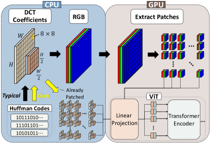
Figure 1: Our proposed training process. The typical process requires full decoding as well as patch extraction to train. In contrast, our process does not since the DCT coefficients are already saved in block-wise fashion. As ViTs work on image patches, we can directly feed these coefficients to the network.

Adapting a CNN architecture designed for RGB inputs to instead receive DCT is nontrivial. The DCT representation of an $H\times W\times 3$ RGB image consists of a $\frac{H}{8}\times\frac{W}{8}\times 8\times 8$ tensor of luma data and two $\frac{H}{16}\!\times\frac{W}{16}\times 8\times 8$ tensors of chroma data. The CNN architecture must be modified both to accept lower-resolution inputs (e.g. by skipping the first few stages of a ResNet50 and adding capacity to later stages) and to accept heterogeneously-sized luma and chroma data (e.g. by encoding them with separate pathways).

We overcome these challenges by using Vision Transformers (ViTs) [5] rather than CNNs. ViTs use a patch embedding layer to encode non-overlapping image patches into vectors, which are processed using a Transformer [6]. This is a perfect match to DCT representations, which also represent non-overlapping RGB image patches as vectors. We show that ViTs can be easily adapted to DCT inputs by modifying only the initial patch embedding layer and leaving the rest of the architecture unchanged.

Data augmentation is critical for training accurate networks; this is especially true for ViTs [7, 8, 9]. However, standard image augmentations such as resizing, cropping, flipping, color jittering, etc. are expressed as transformations on RGB images; prior work [1, 2] on neural networks with DCT inputs thus implement data augmentation by converting DCT to RGB, augmenting in RGB, then converting back to DCT before passing the image to the network. This negates all of the potential training-time efficiency gains of using DCT representations; improvements can only be realized during inference when augmentations are not used.

We overcome this limitation by augmenting DCT image representations directly, avoiding any DCT to RGB conversions during training. We show how all image augmentations used by RandAugment [10] can be implemented on DCT representations. Some standard augmentations such as image rotation and shearing are costly to implement in DCT, so we also introduce several new augmentations which are natural for DCT.

Using these insights, we train ViT-S and ViT-Ti models on ImageNet [11, 12] which match the accuracy of their RGB counterparts. Compared to an RGB equivalent, our ViT-Ti model is up to 39.2% faster per training iteration and 17.9% faster during inference. We believe that these results demonstrate the benefits of neural networks that ingest frequency-domain image representations.

2 Related Work

Training in the frequency domain is extensively explored in the recent studies. They consider JPEG [1, 2, 13, 14, 15, 16, 17, 18, 19, 20, 21], DCT [22, 23, 24, 25, 26, 27, 28, 29] or video codecs [30, 31, 32, 33] with a primary focus on increasing the throughput of the model by skipping most of the decoding steps. Many of these works base their model architecture on CNNs. However, adapting CNNs to accept frequency input requires nontrivial modification to the architecture [1, 2, 17, 18, 30]. More recent studies [34, 35] explore training from a neural compressor [36, 37, 38, 39, 40, 41, 42, 43, 44, 45] instead of an existing compression algorithms [46, 47, 48, 49]. This approach, however, requires transcoding the existing data to their neural compressed format, increasing overhead. We instead use Vision Transformers [5, 7, 8, 50] on the JPEG-encoded data. Our approach has two advantages: (1) patch-wise architecture of ViTs is better suited for existing compression algorithms, (2) does not require any transcoding; it can work on any JPEG images.

Data augmentation directly on the frequency domain has been studied in several works. Gueguen et al. [1] suggested augmenting on RGB and converting back to DCT. Wiles et al. [34] used an augmentation network that is tailored towards their neural compressor. Others focus on a more classical approach such as sharpening [51, 52, 53, 54, 55, 56, 57], resizing [58, 59, 60, 61, 62, 63, 64, 65], watermarking [66, 67, 68, 69, 70, 71, 72], segmentation [73, 74, 75, 76, 77], flip and 90-degree rotation [78, 21], scalar operations [79], and forgery detection [80, 81, 82] via analyzing the properties of JPEG and DCT. However, to our knowledge, no other works have thoroughly studied the effect of DCT augmentation during frequency-domain training.

Speeding up ViTs has been rigorously studied. These either utilize CNN-hybrid architectures to reduce computation [83, 84, 85, 86, 87, 88, 89], speed up attention by sparsifying [90, 91, 92, 93], linearizing [94, 95], or through other techniques such as pruning [96, 97, 98, 99], bottlenecking [100], or approximation [101]. While we only consider the plain ViT architecture in this paper, we want to emphasize that faster data loading is imperative to fully take advantage of these speed-ups as models can only infer as fast as the data loading speed.

3 Background

Here, we discuss Discrete Cosine Transform (DCT) and JPEG compression process. They are crucial to designing a model and DCT data augmentations in the later sections.

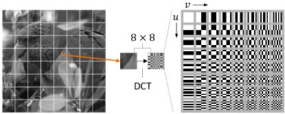
Figure 2: Process of applying $8\times 8$ DCT to the input image. The input image is sliced into $8\times 8$ patches and the DCT is applied to each patch. The DCT bases are shown on the right.

Discrete cosine transform decomposes a finite data sequence into a sum of discrete-frequency cosine functions. It is a transformation from the spatial domain to the frequency domain. We will focus on $8\times 8$ DCT since it is a transform used in JPEG. Let $x\in\mathbb{R}^{8\times 8}$ be a $8\times 8$ image patch. Then its DCT transform $X\in\mathbb{R}^{8\times 8}$ is given by:

Where $\alpha_{i}=1/\sqrt{2}$ if $i=0$, else $1$, $u,v,m,n\in[0..7]$. Figure 2 shows how the DCT is applied to an image in JPEG. The original image patch can be reconstructed by a weighted sum of the DCT bases (Fig. 2) and their corresponding coefficients $X_{u,v}$. For the standard JPEG setting, the pixel-space min/max value of $[-128,127]$, is scaled up by $8\times$ to $[-1024,1016]$. The proof of this property is shown in Appendix A. This property is necessary to implement several DCT augmentations in Sec. 5.

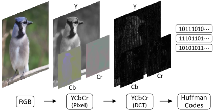
Figure 3: A simplified JPEG compression process. An RGB image is first converted to YCbCr, then transformed to DCT space. They are then encoded into binary codes and written to disk. Decoding follows the inverse of this process.

JPEG [46, 102, 47] is a widely used compression algorithm that is designed to encode images generated by digital photography. The encoding process is as follows:

1. $H\times W\times 3$ RGB image is given as input

2. RGB is converted to YCbCr color space

3. CbCr channels are downsampled to $\frac{H}{2}\times\frac{W}{2}$

4. Values are shifted from [0,255] to [-128,127]

5. DCT is applied to non-overlapping $8\times 8$ pixel patches

6. DCT coefficients are quantized

7. Run-length encoding(RLE) compresses the coefficients

8. RLE symbols are encoded using Huffman coding

A simplified illustration of this process is shown in Figure 3. YCbCr is a color space where Y represents luma (i.e. brightness) and Cb, Cr signifies chroma (i.e. color) of the image. Step (e) produces a data of size $\mathbf{Y}\in\mathbb{R}^{1\times\frac{H}{8}\times\frac{W}{8}\times 8\times 8},\mathbf{U}\in\mathbb{R}^{2\times\frac{H}{16}\times\frac{W}{16}\times 8\times 8}$ for Y and CbCr channel respectively. These $8\times 8$ DCT coefficients are referred to as DCT Blocks in the later sections.

Compute cost to decode JPEG can be analyzed by counting the number of operations (OPs) for the inverse of the above process. Consider decoding a single $8\times 8$ patch. Our proposed scheme decodes step (h) - (f) with a computation cost of $3N_{s}+128$ OPs where $N_{s}\in[1..64]$: number of RLE symbols. Full JPEG decoding, on the other hand, requires $3N_{s}+1717$ OPs. If we suppose $N_{s}=32$, then the compute cost is $224$ and $1813$ OPs respectively, where our scheme theoretically saves computation by $87.6\%$. The details of these values are shown in Appendix B.

4 Model Architecture

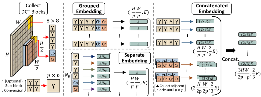
Figure 4: Proposed embedding strategies. We first collect $8\times 8$ DCT blocks until it matches the patch size. Then, these blocks can be embedded using one of the strategies. Grouped embedding groups all of the collected blocks and embeds them together. Separate embedding embeds each block separately and mixes it. Concatenated embedding embeds $\mathbf{Y}$ and $\mathbf{U}$ separately and concatenates them.

Designing a neural network that works on JPEG-encoded DCT coefficients can be challenging. In Fig. 3, we showed that JPEG downsamples CbCr channels to $\frac{H}{2}\times\frac{W}{2}$. This spatial disparity must be addressed before training in DCT. An existing work by Gueguen et al. [1] suggested several new CNN architectures which include (1) upsampling, (2) downsampling, and (3) late-concatenation. The first two architectures either upsample CbCr to match the dimension of Y or downsample Y to match CbCr. However, doing so results in (1) redundant computation or (2) loss of information due to resizing. The third approach, late-concatenation, computes them separately and concatenates them further down the network. However, this requires substantial modification of the CNN architecture, making adaptation to existing models difficult.

We believe that ViTs are better suited to deal with this unique characteristic of JPEG. Vision transformers work on patches of an image [5, 7, 8, 9]. Considering that JPEG DCT already extracts $8\times 8$ patches from an image (Fig. 3 (e)), we can employ them by modifying only the initial embedding layer. This allows easier integration into other ViTs as the rest of the architecture can remain untouched.

Therefore, in this section, we propose several patch-embedding strategies that are plausible solutions to this problem. These modified patch embedding layers are illustrated in Fig. 4. The architecture that follows is identical to the plain ViT defined in [5, 50, 7].

Grouped embedding generates embeddings by grouping the $8\times 8$ DCT blocks together from the corresponding patch position. Consider a DCT input $\mathbf{Y},\mathbf{U}$ defined in Fig. 3. Grouped embedding collects DCT blocks such that for patch size $p$ , $\mathbf{Y}\rightarrow\mathbf{Y}_{r}\in\mathbb{R}^{\frac{H}{p}\times\frac{W}{p}\times p^{2}}$ and $\mathbf{U}\rightarrow\mathbf{U}_{r}\in\mathbb{R}^{\frac{H}{p}\times\frac{W}{p}\times\frac{2p^{2}}{4}}$ where the channel and block size are flattened to the last dimension. Then, this is concatenated along the last axis as $(\mathbf{Y}_{r},\mathbf{U}_{r})\rightarrow\mathbf{YU}_{r}\in\mathbb{R}^{\frac{H}{p}\times\frac{W}{p}\times\frac{3p^{2}}{2}}$ which will then be embedded as $\mathbf{z}:\mathbf{YU}_{r}\rightarrow\mathbf{z}\in\mathbb{R}^{\frac{HW}{p\cdot p}\times E}$ where $\mathbf{z}$ is the generated embedding and $E$ is the embedding size.

Separate embedding generates separate embeddings for each DCT block in a patch. A DCT input $\mathbf{Y},\mathbf{U}$ is reshaped as $\mathbf{Y}\rightarrow\mathbf{Y}_{r}\in\mathbb{R}^{\frac{H}{p}\times\frac{W}{p}\times\frac{p^{2}}{64}\times 64},\mathbf{U}\rightarrow\mathbf{U}_{r}\in\mathbb{R}^{\frac{H}{p}\times\frac{W}{p}\times\frac{2p^{2}}{4\cdot 64}\times 64}$ which is embedded separately for each block: $(\mathbf{Y}_{r},\mathbf{U}_{r})\rightarrow\mathbf{z}\in\mathbb{R}^{\frac{HW}{p\cdot p}\times\frac{3p^{2}}{2\cdot 64}\times\frac{E}{N_{B}}}$ where $N_{B}$ = number of blocks = $\frac{3p^{2}}{2\cdot 64}$. This is then mixed using a linear layer to generate a final embedding $\mathbf{z}\rightarrow\mathbf{z}\in\mathbb{R}^{\frac{HW}{p\cdot p}\times E}$. Our intuition behind this strategy is that the information each block holds might be critical, thus training a specialized linear layer for each block could yield better results.

Concatenated embedding embeds and concatenates the DCT blocks from $\mathbf{Y}$, $\mathbf{U}$ separately. Our intuition is that since $\mathbf{Y}$ and $\mathbf{U}$ represent different information (luma and chroma), designing specialized layers that handle each information separately may be necessary. However, this generates more embeddings per image patch than the plain model. To keep the overall size even, we reduce the size of each embedding to 2/3. An embedding formula is $\mathbf{Y}\rightarrow\mathbf{Y}_{r}\in\mathbb{R}^{\frac{H}{p}\times\frac{W}{p}\times p^{2}},\mathbf{U}\rightarrow\mathbf{U}_{r}\in\mathbb{R}^{2\times\frac{H}{2p}\times\frac{W}{2p}\times p^{2}}$, which is then embedded separately per channel type: $\mathbf{Y}_{r}\rightarrow\mathbf{z}_{Y}\in\mathbb{R}^{\frac{HW}{p\cdot p}\times\frac{2E}{3}},\mathbf{U}_{r}\rightarrow\mathbf{z}_{U}\in\mathbb{R}^{\frac{2HW}{4p\cdot p}\times\frac{2E}{3}}$ then concatenated $(\mathbf{z}_{Y},\mathbf{z}_{U})\rightarrow\mathbf{z}\in\mathbb{R}^{\frac{3HW}{2p\cdot p}\times\frac{2E}{3}}$ to generate an embedding $\mathbf{z}$.

Sub-block conversion [64] can be applied as an alternate way to embed a patch. Consider ViT architecture of patch size 16. For simplicity, assume only the Y channel is present. To form a patch size of $16\times 16$, four $8\times 8$ DCT blocks have to be grouped together. One strategy is to embed these directly through the linear layer. Another approach is to convert them into a single $16\times 16$ block and embed them. In other words, we embed the DCT patches from a $16\times 16$ DCT. There exists a way to efficiently extract these $16\times 16$ DCT from the smaller $8\times 8$ DCT blocks and vice versa known as sub-block conversion [64]. This technique can allow us to extract a native DCT patch of different sizes, potentially yielding better results. We also use this technique to implement several augmentations in Sec. 5.

5 DCT Augmentation

Data augmentation has been a vital component in training robust networks [10, 103, 104, 105, 106, 107, 108]. However, augmenting the DCT, as well as training with it, has not been studied in depth. There exist several prior works for some augmentations such as sharpening or resizing as discussed in Sec. 2, but most other RGB augments lack their DCT counterparts.

Existing work by Gueguen et al. [1] proposed converting DCT to RGB, augmenting in RGB, and converting it back to DCT. However, this incurs expensive RGB/DCT conversion as shown in Sec. 3. More recent work by Wiles et al. [34] used a specialized augmentation network that augments their neural-compressed format. Doing so, however, sacrifices versatility as it requires training and can’t be reliably generalized to other resolutions or data.

Our approach is different. We instead implement augmentations directly on DCT by analyzing its properties. That way, we can avoid converting to RGB or relying on a trained augmentation network. In other words, our method is fast, flexible, and works on virtually any data, so long as it is represented in DCT. Thus, in this section, we implement all augmentations used in RandAugment [10] as well as suggest new augmentations that are meaningful for DCT. We mark the ones we suggest using an asterisk(*).

There are largely two different types of DCT augmentation: photometric and geometric. Each of which uses different key properties of the DCT. While these augmentations are not meant to precisely reproduce RGB augmentations, most of our implementations approximate the RGB counterparts reasonably well. The overview of the augmentations and their similarity metrics are shown in Fig. 6.

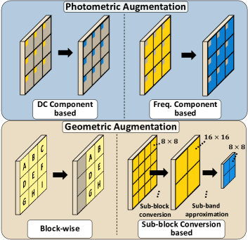
Figure 5: A visualization of different DCT augmentation types. Orange-colored coefficients are augmented and saved as blue. The bottom two examples illustrate Translate and Resize.

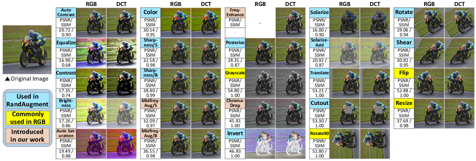
Figure 6: A visualization of RGB augmentations and their DCT counterparts. ‘/S’ or ‘/B’ indicates ‘sharpen’ or ‘blur’ on sharpness-related augmentations. Resize has been compared where they scale the image up by 2. PSNR and SSIM are calculated for each DCT augmentation. We observe that most DCT augmentations resemble RGB augmentations. Augmentations such as grayscale, cutout, and flip are identical to RGB. However, other augmentations including equalize and contrast are not exactly equal to RGB.

5.1 Photometric augmentation

Photometric augmentation alters a metric of an image, which includes brightness or sharpness. Our implementation of this can be roughly categorized into two: DC component-based and frequency component-based augmentation. Both use the attributes of a DCT coefficient.

DC Component-based augmentation only alters the DCT coefficient without frequency ($X_{0,0}$), which is simply a scaled sum of all pixel values in the block (Eq. 3.1). Altering this value will affect all pixels in the block evenly. This property can be used in two ways – either when we have to modify a value uniformly across all pixels, or when we have to approximate a value of the pixels in a block.

Brightness augmentation alters the brightness of the image. Considering that the image is represented in YCbCr color space, we can implement this augmentation by simply modifying the DC component of the Y channel. Let $Y_{u,v}^{h,w}$ denote a $u,v$-th DCT coefficient of Y at block position $h,w$. Then our implementation $f$ is the following where $t\in\mathbb{R}$.

Contrast modifies the distance between the bright and dark values in the image. Since DCT coefficients are zero-centered by design (Fig. 3 (d)) and the brightness of a block can be approximated using the DC component $Y_{0,0}$, we can categorize the non-negative component as ‘bright’ and the negative component as ‘dark’. Therefore, multiplying $Y_{0,0}$ with $t\in[0,\infty)$ can adjust the contrast of the image. The implementation is $f:Y_{0,0}^{h,w}\rightarrow tY_{0,0}^{h,w}$. Similarly, Equalize applies histogram equalization to $Y_{0,0}$.

Color (Saturation) augmentation apply the same equation of Contrast to $U$ (DCT coefficient of CbCr), instead of $Y$. This augments the saturation as illustrated in Fig. 6.

AutoContrast scales the values so that the brightest and darkest value in an image becomes the brightest and darkest possible value. These values are approximated using $X_{0,0}$ in the same way as Contrast. In Eq. 3.1, we showed that the min/max value of the DCT in JPEG is $[-1024,1016]$. Thus, our implementation $f$ is as follows.

AutoSaturation^∗ applies the formula in AutoContrast to $U$. This allows the DCT to utilize the full range of the color.

Frequency component-based augmentation uses non-DC components ($X_{u,v},\,u,v\neq 0$). Altering the amplitude of these changes the intensity of the corresponding cosine signal in the pixel space. Here, we designed three augmentations each affecting frequency differently.

Sharpness augmentation adjusts a sharpness of an image. Typically in RGB, this utilizes a convolution kernel to achieve such an effect. However, in DCT, several studies show that this can be implemented by adjusting the frequency components of the DCT [52, 53, 54, 51, 55, 56, 57]. They show that sharper images will generally have a higher frequency as there are more sudden changes around the sharp edges. Using this property, we implement Sharpness by linearly altering the frequency components. If $t>0$, the following equation sharpens the image. Otherwise, it blurs it.

MidfreqAug^∗ augmentation is similar to sharpness but instead of peaking the augmentation strength at the highest frequency $(u,v=7)$, we peaked it at the middle frequency $(u,v\in\{3,4\})$. We expect the results to be similar to Sharpness, but possibly with less noise.

FreqEnhance^∗ multiplies all frequency components uniformly with a positive factor $t\in[0,\infty)$. The augmentation is simply $f:Y_{u,v}^{h,w}\rightarrow tY_{u,v}^{h,w},\;u,v\neq 0$. We believe that this allows us to see the impact of a frequency component with respect to the model performance.

Photometric – special case. There are some augmentations that do not categorize into either of the above augmentations. Invert simply flips the sign of all DCT coefficients. This is because the coefficients are virtually zero-centered. Posterize quantizes $X_{0,0}$ to lower bits. Solarize uses $X_{0,0}$ to determine whether or not the DCT block should be inverted. SolarizeAdd adds a preset value to $X_{0,0}$ if it is below threshold. Grayscale replaces $U$ with zeros, removing color information. ChromaDrop^∗ instead drops the Cb or Cr channel randomly, removing only half of the color information.

5.2 Geometric augmentation

Geometric augmentation modifies the image plane geometrically. An example of this augmentation includes translation, rotation, or shearing. There are two main sub-categories of geometric augmentation – block-wise and sub-block conversion-based augmentation.

Block-wise augmentation treats the DCT block positions similarly to pixel positions. Translate can be implemented by moving the positions $h,w$ of each $X^{h,w}$ and filling the blank with zeros. Cutout follows a similar process where we crop blocks out and fill them with zeros.

Flipping the DCT coefficients utilize the fact that odd-column or odd-row DCT bases are odd-symmetric [78]. Flip is performed by flipping the position of the blocks and then flipping the individual DCT blocks. Define $R=\texttt{diag}(1,-1,1,-1,...-1)$ of matching size. Then, the per-block flipping operation is as follows.

$$f^{X}:X^{h,w}\rightarrow\bigg{\{}\begin{array}[]{ll}X^{h,w}R&\text{if horizontal flip}\\ RX^{h,w}&\text{if vertical flip}\end{array}\bigg{\}}$$ (5.4)

Rotate90 is implemented using a transpose with flipping [78]. We first rotate the block position $h,w$ and rotate each $X^{h,w}$ by 90 degrees. The per-block rotation is defined as:

Sub-block conversion-based augmentation uses the relationship between the DCT block and its smaller sub-blocks. This allows us to efficiently calculate the DCT of different DCT bases without the need to do inverse transform (e.g. $8\times 8$ DCT$\leftrightarrow 32\times 32$ DCT). The relationship studied by Jiang and Feng [64] is as follows. Let $X_{N\times M}^{h,w}$ be the DCT coefficient block of $N\times M$ DCT at block position $h,w$. Then, there exists a conversion matrix $A$ such that:

Where $A_{L,N}$ is a $LN\times LN$ matrix that converts the $L$ number of $N$ 1-D DCT blocks into a single $LN$ DCT block. The decomposition of $X_{LN\times MN}$ DCT blocks into $L\times M$ DCT blocks of $X_{N\times N}$ follows a similar process:

Derivation of $A$ is given in the Appendix C.

Resize can be implemented if we can understand how to resize individual DCT blocks. Suppose that there exists a way to resize $X_{4\times 4}$ to $X_{8\times 8}$ by padding. Then, to upsample $X_{8\times 8}$ while keeping the $8\times 8$ sliced structure of JPEG DCT, we can first decompose $X_{8\times 8}$ into four $X_{4\times 4}$ using sub-block conversion. Then, we can individually resize each $X_{4\times 4}$ to $X_{8\times 8}$. This gives us four $X_{8\times 8}$ blocks upsampled from one $X_{8\times 8}$. Downsampling can follow a similar process. We first combine four adjacent $X_{8\times 8}$ into a single $X_{16\times 16}$ using sub-block conversion. Then, we resize $X_{16\times 16}$ down to $X_{8\times 8}$. This process is shown in Fig. 5.

This technique to resize each individual DCT block is known as sub-band approximation and has been studied by Mukherjee and Mitra [65]. Their work shows that if $X_{N\times N}(k,l)$ is a $(k,l)$-th coefficient of a $X_{N\times N}$ block, then, the approximate relationship is:

Using this, we can upsample $L\times M$ times by resizing each $X_{N\times N}$ to $X_{LN\times MN}$ and decomposing them to $L\times M$ $X_{N\times N}$. $L\times M$ downsampling combines $L\times M$ adjacent $X_{N\times N}$ to form $X_{LN\times MN}$ and resize it to $X_{N\times N}$. An arbitrary resizing of $\frac{P}{Q}\times\frac{R}{S}$ can be done by first upsampling $P\times R$ times and downsampling the result by $Q\times S$.

Architecture	Color Space	Aug. Space	Embed. FLOPs	Decode	Augment	Train Data Load	Model Fwd/Bwd	Train Pipeline	Eval Data Load	Model Fwd	Eval Pipeline	Val Acc (%)
($\downarrow$ Performance)				Latency per img (ms)		Throughput per GPU (FPS)
ViT-Ti [50]	RGB	RGB	28.9M	3.68	3.08	571.5	832.8	493.8	641.4	2898.7	638.0	74.1
ViT-S [50]	RGB	RGB	57.8M	3.62	3.01	558.0	355.7	352.1	660.2	1174.5	610.5	76.5
ViT-S★ [50]	RGB	RGB	57.8M	3.69	2.63	574.7	716.8	489.0	680.3	2335.1	644.2	75.6
SwinV2-T★ [109]	RGB	RGB	20.8M	3.61	2.98	489.8	231.5	231.6	614.8	809.5	516.2	79.0⋆
ResNet50[110]	RGB	RGB	-	-	-	-	-	-	688.2	1226.8	639.1	76.1
JPEG-Ti	DCT	DCT	16.1M	1.42	2.62	816.2	857.2	687.6	775.3	2847.5	752.3	75.1
JPEG-S	DCT	DCT	30.5M	1.49	2.40	824.8	364.3	360.5	782.9	1139.7	711.1	76.5
JPEG-S★	DCT	DCT	30.5M	1.42	2.37	821.7	764.0	665.8	793.1	2384.1	711.8	75.8
JPEG-S★♢	DCT	RGB to DCT	30.5M	3.62	5.98	425.3	751.9	372.3	748.7	2382.4	721.0	76.3
SwinV2-T★	DCT	DCT	13.0M	1.40	2.47	752.0	241.9	235.9	664.2	824.9	578.0	79.4
ResNet50♢[1] [2]	DCT	RGB to DCT	-	-	-	-	-	-	785.7	5969.8	753.5	76.1
($\downarrow$ Improvements)			(Reduction $\blacktriangledown$)			(Speed-ups $\blacktriangle$)
JPEG-Ti vs ViT-Ti			-44.4 %	-61.4 %	-14.9 %	+42.8 %	+2.9 %	+39.2 %	+20.9 %	-1.8 %	+17.9 %	+1.0
JPEG-S vs ViT-S			-47.2 %	-58.8 %	-20.3 %	+47.8 %	+2.4 %	+2.4 %	+18.6 %	-3.0 %	+16.5 %	+0.0
JPEG-S★ ViT-S★			-47.2 %	-61.5 %	-9.9 %	+43.0 %	+6.6 %	+36.2 %	+16.6 %	+2.1 %	+10.5 %	+0.2
JPEG-S★ vs JPEG-S★♢			+0.0 %	-60.8 %	-60.4 %	+93.2 %	+1.6 %	+78.8 %	+5.9 %	+0.1 %	-1.3 %	-0.5
SwinV2-T★ (DCT vs RGB)			-37.7 %	-61.2 %	-17.1 %	+53.5 %	+4.5 %	+1.9 %	+8.0 %	+1.9 %	+12.0 %	+0.4

Table 1: Model throughput per GPU for each pipeline element and accuracy. Embed. FLOPs shows the FLOPs needed to generate patch embeddings. Decode and Augment indicates the per-image processing latency during training. Val Acc shows the accuracy on the ImageNet validation set. ‘JPEG-’ prefix indicates that it is a ViT trained using JPEG DCT coefficients. Model with ‘$\bigstar$’ symbol is trained using mixed precision [111]. ‘$\diamondsuit$’ models are trained using the pipeline suggested by Gueguen et al. [1]. ^⋆SwinV2 models are trained using the same recipe as in [50] for a fair comparison. The details of these measurements are shown in Appendix K.

Rotate is implemented using the rotational property of the Fourier transform [112, 113, 114]. This property denotes that the Fourier transform of a rotated function is equal to rotating the Fourier transform of a function. To use this property, we slightly alter the Eq. 5.6. Instead of combining the blocks to $X_{LN\times MN}$ DCT, we combine them to the discrete Fourier transform (DFT) coefficients. Define $D_{N\times N}$ as the DFT coefficient block of size $N\times N$. Then, the rotation is done by combining $L\times M$ $X_{N\times N}$ to $D_{LN\times MN}$, rotating it, and decomposing it back to $L\times M$ $X_{N\times N}$ using the modified Eq. 5.7. This can be further improved using the lossless 90-degree rotation to minimize the lossy arbitrary-degree rotation. The details of this DFT conversion are shown in Appendix F.

Shear is identically implemented as Rotate where instead of rotating $D_{LN\times MN}$, we shear it. This is because we can apply the same property [112] for each axis.

6 Experiments

In this section, we compare our models trained in DCT space with the RGB models. We show that the DCT models achieve similar accuracy but perform notably faster than the RGB models. First, we compare the throughput and accuracy of the RGB and DCT models. Then, we compare the DCT embedding strategies covered in Sec. 4. Lastly, we conduct an ablation study on the DCT data augmentation.

		Photometric			Geometric		Accuracy
Subset	Resize	DC based	Freq. based	Special case	Block-wise	Sub-block based	RGB	DCT
(Avg. latency (ms) $\downarrow$)
RGB	2.17	0.61	1.34	0.67	1.23	1.28	-	-
DCT	2.79	0.37	0.54	0.34	0.42	9.31	-	-
(Ablation $\downarrow$)
All	✓	✓	✓	✓	✓	✓	76.5	74.6
No sub-block	✓	✓	✓	✓	✓	✗	76.2	75.1
No block-wise	✓	✓	✓	✓	✗	✗	76.0	72.6
No Special-case	✓	✓	✓	✗	✗	✗	76.3	73.3
No Freq. based	✓	✓	✗	✗	✗	✗	75.9	74.2
No DC based	✓	✗	✗	✗	✗	✗	74.4	75.5
Best Subset	✓	Brightness, Contrast, Color, AutoContrast, AutoSaturation, Sharpness, MidfreqAug, Posterize, Grayscale, ChromaDrop, Translate, Cutout, Rotate90				✗	76.5⋆	76.5

Table 2: Data augmentation ablation study on ViT-S. At the bottom row, we report the best subset we found and train both the RGB and DCT models from it. ^⋆RGB accuracy is obtained with MidfreqAug removed, since it is analogous to Sharpness in RGB as shown in Fig. 6.

Grouped	Separate	Concat.	Sub-block	Acc
✓	-	-	✓	76.5
-	✓	-	✓	74.7
-	-	✓	✓	71.3
✓	-	-	-	74.6
-	✓	-	-	73.8
-	-	✓	-	71.3

Table 3: Embedding strategy ablation study on ViT-S. We see that grouped embedding with sub-block outperforms other strategies.

Implementation Details. All experiments are conducted with PyTorch [115]. We extract DCT coefficients using a modified version of libjpeg [116] and TorchJPEG [117]. All timing measurements are performed using $2\times$ A40 GPUs and 8 cores from an Intel Xeon 6226R CPU, and all throughputs are reported per GPU. We used fvcore [118] to obtain the FLOPs. All models are trained on ImageNet [11, 12], which we resize on-disk to $512\times 512$ prior to training. We re-implement a ViT training pipeline in PyTorch, carefully following the recipe suggested by Beyer et al. [50] which uses random resized crop, random flip, RandAugment [10] and Mixup [119] with a global batch size of 1024. All plain ViT models are trained with a patch size of 16. SwinV2 model [109] uses a patch size of 4, a window size of 8, and a global batch size of 512. ‘-S’ models are trained for 90 epochs. ‘-Ti’ and SwinV2 models are instead trained for 300 epochs using the same recipe in [50]. Following [50], we randomly sample 1% of the train set to use for validation. Our RGB ResNet-50 baseline uses the V1 weights from Torchvision [110]. There exist recent works with improved training recipes for ResNets [120, 121], but this is orthogonal to our work. The DCT ResNet-50 uses the model proposed by Gueguen et al. [1] and Xu et al. [2].

6.1 Main results

The hyperparameter settings for the models are given in Appendix J. Tab. 1 shows the comprehensive result from our experiment. Both the ViT and CNN models show equivalent accuracy to their RGB counterparts. However, loading directly from JPEG DCT reduces decoding latency by up to 61.5%. We see a similar effect on the augmentation latency to a lesser extent. Additionally, as the input size has been halved by JPEG (Fig. 3), we observe that the FLOPs needed to generate embeddings are reduced by up to 47.2%. These speed-ups boost throughput for DCT models. Most notably, our JPEG-Ti model showed 39.2% and 17.9% faster training and evaluation. Our augmentation scheme improves train data loading throughput by 93.2% versus the one by Gueguen et al. [1], which must convert DCT to RGB, augment, and convert it back to DCT.

While training as-is still reaps the benefits of faster data loading, we can observe that the JPEG-S model is bottlenecked by model forward and backward passes. One option is to employ mixed precision training [111]. This allows us to fully realize the data loading speed-ups by accelerating the model with minor accuracy loss. We observe that our JPEG-S model trained using mixed precision is 36.2% faster during training time compared to the RGB counterpart. We believe most other faster models discussed in Sec. 2 will also benefit from this speed-up.

6.2 Embedding strategies

To see which patch embedding scheme is most suitable for DCT, we performed an ablation study in Tab. 3. We ablate on the embedding strategies and the sub-block conversion technique discussed in Sec. 4 on ViT-S. The results show two things. One is that the simplest strategy–grouped embedding–is best, and that sub-block conversion is important to achieve high accuracy. We believe this indicates that (1) all blocks in an image patch relay information of that patch as a whole; they should not be separately inferred, and (2) it is more natural for the model to deduce the information in a patch if the sub-blocks are fused together. The best strategy is used throughout the DCT models in Tab. 1.

6.3 Augmentation

As discussed in Sec. 5, data augmentation is crucial to train a well-performing model. However, many existing studies [103, 104, 105, 106, 107, 108, 9, 10] are tuned toward RGB augmentations; we cannot assume that the existing work’s result would be consistent on DCT. In other words, some DCT augmentations could have a different impact on both the accuracy and throughput of the model compared to RGB. Therefore, we perform an ablation study on data augmentations discussed in Sec. 5 and report the result in Tab. 2. We perform ablation by varying the subset of augmentations used in RandAugment [10] on ViT-S. The experiment is performed separately for RGB and DCT with their respective augmentation sets. The results show that while sub-block-based augmentations (e.g. rotate, shear) are prohibitively expensive to do directly on DCT, it is not as important to train a model. We report the best augmentation subset we found without sub-block-based augmentations at the bottom row. In addition, we train an RGB model using this subset and compare the accuracy. We can see that the RGB model performs identically to the DCT model, and the subset does not unfairly favor DCT over RGB models.

7 Conclusion

In this paper, we demonstrated that vision transformers can be accelerated significantly by directly training from the DCT coefficients of JPEG. We proposed several DCT embedding strategies for ViT, as well as reasonable augmentations that can be directly carried out on the DCT coefficients. The throughput of our model is considerably faster with virtually no accuracy loss compared to RGB.

RGB has been widely used for as long as computer vision existed. Many computer vision schemes regard retrieving RGB as a necessary cost; they have not considered the potential of direct encoded-space training in-depth. We wanted to show the capability of this approach, as well as demonstrate that recovering RGB is not always necessary.

Encoded-space training can be adapted to nearly all scenarios that require loading some compressed data from storage. From mobile devices to powerful data centers, there are no situations where they wouldn’t benefit from faster loading speed. As we only considered the plain ViT architecture, there is still more to be gained by adapting our findings to the existing efficient architectures. Future studies may also consider a better augmentation strategy to improve the performance further. We hope that the techniques shown in this paper prove to be an adequate foundation for future encoded-space research.

A Scaling property of a $8\times 8$ DCT

Consider an $8\times 8$ 2D-DCT defined as the following where $\alpha_{i}=1/\sqrt{2}$ if $i=0$, else $1$, $u,v,m,n\in[0..7]$.

We then calculate how much the DCT scales up the min/max values considering the following two cases.

• If $u,v=0$
  If $u,v=0$ then the resulting coefficient $X_{0,0}$ is simply:

  $$X_{0,0} =\frac{1}{8}\sum_{m=0}^{7}\sum_{n=0}^{7}x_{m,n}\cdot\cos(0)\cos(0)$$ (A.2)

  $$=\frac{1}{8}\sum_{m=0}^{7}\sum_{n=0}^{7}x_{m,n}\hskip 8.5359pt(\because\cos(0)=1)$$ (A.3)

  Which is minimized/maximized when $x_{m,n}$ is min/max:

  $$\min(X_{0,0}) =\frac{1}{8}\min(x_{m,n})\cdot 8\cdot 8$$ (A.4)

  $$=\min(x_{m,n})\cdot 8$$ (A.5)

  $$\max(X_{0,0}) =\frac{1}{8}\max(x_{m,n})\cdot 8\cdot 8$$ (A.6)

  $$=\max(x_{m,n})\cdot 8$$ (A.7)

  So applying $8\times 8$ DCT to an input with min/max value of [-128, 127] scales the output min/max value to:

  $$\min(X_{0,0}) =-128\cdot 8=-1024$$ (A.8)

  $$\max(X_{0,0}) =127\cdot 8=1016$$ (A.9)

• If $u\neq 0$ or $v\neq 0$
  In this case, the amplitude of DCT coefficient $X_{u,v}$ will be maximized if the input data sequence resonates with (i.e. match the signs of) the cosine signal of the corresponding DCT bases. We will show that this value is less than or equal to the magnitude when $u,v=0$. We first consider the 1D case and then use it to calculate the 2D case. The 1D DCT is as follows.

  $$X_{u} =\frac{\alpha_{u}}{2}\sum_{m=0}^{7}x_{m}\times\cos\bigg{[}\frac{\pi(2m+1)u}{16}\bigg{]}$$ (A.10)

  Where the DCT bases are:

  $$\frac{\alpha_{u}}{2}\cos\bigg{[}\frac{\pi(2m+1)u}{16}\bigg{]},\hskip 8.5359ptm,u\in[0..7]$$ (A.11)

  This 1D DCT will be maximized when the signs of $x_{m}$ match the signs of the DCT bases. Likewise, it will be minimized when the signs are exactly the opposite. Therefore, we compare the absolute sum of the DCT bases and show that it is less than or equal to the sum when $u=0$. This absolute sum of DCT bases can be interpreted as the scale-up factor as it shows how much the input 1’s with matching signs are scaled up. The following values are rounded to the third decimal place.

  • $u=0$: $\displaystyle X_{0}=\frac{\alpha_{0}}{2}\sum_{m=0}^{7}\texttt{abs}(1)=2\sqrt{2}=\mathbf{2.828}$

  • $u=1$: $\displaystyle X_{1}=\frac{\alpha_{1}}{2}\sum_{m=0}^{7}\texttt{abs}(\cos\bigg{[}\frac{\pi(2m+1)}{16}\bigg{]})=2.563$

  • $u=2$: $\displaystyle X_{2}=\frac{\alpha_{2}}{2}\sum_{m=0}^{7}\texttt{abs}(\cos\bigg{[}\frac{2\pi(2m+1)}{16}\bigg{]})=2.613$

  • $u=3$: $\displaystyle X_{3}=\frac{\alpha_{3}}{2}\sum_{m=0}^{7}\texttt{abs}(\cos\bigg{[}\frac{3\pi(2m+1)}{16}\bigg{]})=2.563$

  • $u=4$: $\displaystyle X_{3}=\frac{\alpha_{4}}{2}\sum_{m=0}^{7}\texttt{abs}(\cos\bigg{[}\frac{4\pi(2m+1)}{16}\bigg{]})=2.828$

  • $u=5$: $\displaystyle X_{3}=\frac{\alpha_{5}}{2}\sum_{m=0}^{7}\texttt{abs}(\cos\bigg{[}\frac{5\pi(2m+1)}{16}\bigg{]})=2.563$

  • $u=6$: $\displaystyle X_{3}=\frac{\alpha_{6}}{2}\sum_{m=0}^{7}\texttt{abs}(\cos\bigg{[}\frac{6\pi(2m+1)}{16}\bigg{]})=2.613$

  • $u=7$: $\displaystyle X_{3}=\frac{\alpha_{7}}{2}\sum_{m=0}^{7}\texttt{abs}(\cos\bigg{[}\frac{7\pi(2m+1)}{16}\bigg{]})=2.563$

  We can see that for all $u$, the absolute sums of DCT bases are less than or equal to the sum when $u=0$. 2D DCT is simply a DCT on each axis (rows and columns), so the 2D scale-up factors will be a pairwise product for any pairs of $u$ with replacement. This will still not exceed the value when we choose $u=0$ twice. Therefore, we can conclude that the minimum and maximum values calculated in the $u,v=0$ case will hold for all $8\times 8$ DCT coefficients. Thus, $8\times 8$ DCT will scale up the min/max value by 8.

B Compute cost to decode JPEG

JPEG is decoded through the following steps.

1. Decode Huffman codes to RLE symbols

2. Decode RLE symbols to quantized DCT coefficients

3. De-quantize the DCT coefficients

4. Apply inverse-DCT to the DCT coefficients

5. Shift value from [-128, 127] to [0, 255]

6. Upsample Cb, Cr by $2\times$ for each dimension

7. Convert YCbCr to RGB

We count the number of operations (OPs) for each step:

1. Read $N_{s}$ Huffman codes and recover $N_{s}$ RLE symbols = $N_{s}+N_{s}=2N_{s}$ OPs

2. Read $N_{s}$ RLE symbols and recover $8\times 8$ quantized DCT coefficients = $N_{s}+64$ OPs

3. Multiply $8\times 8$ quantization table element-wise with $8\times 8$ DCT coefficients = $64$ OPs

4. The $8\times 8$ inverse DCT is given as:

   Where

   $$\gamma_{i} =\Bigg{\{}\begin{array}[]{ll}\frac{1}{\sqrt{2}}&\text{if }i=0\vspace{0.1cm}\\ 1&\text{otherwise}\end{array}$$

   • If $m,n\in[1..7]$
     We need $2\cos+10\text{mul}+3\text{add}+3\text{div}$ per step as $\gamma_{i}=1$. Number of OPs: $7\times 7\times 18=882$

   • If $m=0,n\in[1..7]$ or $m\in[1..7],n=0$
     We need $2\cos+10\text{mul}+3\text{add}+4\text{div}+1\text{sqrt}$ per step. OPs: $7\times 20\times 2=280$

   • If $m=0,n=0$
     $2\cos+10\text{mul}+3\text{add}+5\text{div}+2\text{sqrt}$ = $22$ OPs

   Total OPs per $8\times 8$ block: $882+280+22=1184$

5. Add 128 to every elements of $x_{m,n}$ = 64 OPs

6. Upsample $8\times 8$ Cb and Cr block to $16\times 16$: $256\times 2=512$ OPs per 6 blocks. This is because 4 Y blocks are paired with 1 Cb and Cr block. Per-block cost: $512/6=85.3$ OPs.

7. YCbCr is converted to RGB using [47]:

   $$R =Y+1.402(C_{r}-128)$$

   $$G =Y-0.344136(C_{b}-128)-0.714136(C_{r}-128)$$

   $$B =Y+1.772(C_{b}-128)$$

   For three blocks – Y, Cb, and Cr – the number of OPs is $64\times(2\text{add}+6\text{sub}+4\text{mul})=768$. We ignore the cost of rounding and min/max clamping for simplicity. Thus, the per-block cost is $768/3=256$ OPs

Recovering DCT coefficients requires going through steps (a)-(c), where the compute cost sums up to $3N_{s}+128$ OPs. Full decoding requires $3N_{s}+1717.3$ OPs. We can see that most of the decoding cost comes from the inverse-DCT, which costs 1184 OPs to compute. Note that this result is only an estimate and can vary under different settings.

C Conversion matrix for sub-block conversion

The conversion matrix $A$ can be calculated using the basis transform from $L\times M$ number of $N\times N$ DCT bases to $LN\times MN$ DCT bases. Let $T^{N\times N}$ as a 1-D DCT bases of size $N\times N$ then:

$$\hskip-9.0pt\leavevmode\resizebox{190.79385pt}{}{$\displaystyle T^{N\times N}=\sqrt{\frac{2}{N}}\begin{bmatrix}\frac{1}{\sqrt{2}}&\frac{1}{\sqrt{2}}&\cdots&\frac{1}{\sqrt{2}}\\ \cos[\frac{1\pi}{2N}]&\cos[\frac{3\pi}{2N}]&\cdots&\cos[\frac{(2N-1)\pi}{2N}]\\ \vdots&\vdots&\ddots&\vdots\\ \cos[\frac{(N-1)\pi}{2N}]&\cos[\frac{3(N-1)\pi}{2N}]&\cdots&\cos[\frac{(2N-1)(N-1)\pi}{2N}]\end{bmatrix}$}\hskip-3.0pt$$ (C.1)

$T^{N\times N}$ is an orthogonal matrix [122]. Hence,

$$TT^{T}=I\hskip 14.22636ptT^{T}=T^{-1}$$ (C.2)

Define $B_{large}$ as $T^{LN\times LN}$ and $B_{small}$ as a block diagonal matrix of $T^{N\times N}$ with size $LN\times LN$:

$$B_{small}=\begin{bmatrix}T^{N\times N}&\cdots&0\\ \vdots&\ddots&\vdots\\ 0&\cdots&T^{N\times N}\end{bmatrix}$$ (C.3)

Then the conversion matrix $A_{L,N}$ is[64]:

$$B_{large}=A_{L,N}\times B_{small}$$ (C.4)

$$A_{L,N}=B_{large}\times B^{-1}_{small}$$ (C.5)

Where $B_{small}^{-1}=B_{small}^{T}$ due to Eqs. C.2 and C.3. Thus,

$$A_{L,N}=B_{large}\times B_{small}^{T}$$ (C.6)

We can also see that $B_{large}^{-1}=B_{large}^{T}$. Thus,

$$A_{L,N}^{-1} =(B_{large}\times B_{small}^{T})^{-1}$$ (C.7)

$$=(B_{small}^{T})^{-1}\times B_{large}^{-1}$$ (C.8)

$$=B_{small}\times B_{large}^{T}$$ (C.9)

$$=A_{L,N}^{T}$$ (C.10)

D Sub-band approximation

Define $x(m,n)$ as the 2D image data, and $X(k,l)$ as the 2D DCT coefficient of $x(m,n)$ where $m,n,k,l\in[0..N-1]$. Then, define $x_{LL}(m^{\prime},n^{\prime})$ as the $2\times$ downsized image of $x(m,n)$. Then $x_{LL}$ is given as:

$$x_{LL}(m^{\prime},n^{\prime})=\frac{1}{4}\{x(2m^{\prime},2n^{\prime})+x(2m^{\prime}+1,2n^{\prime})+\\ x(2m^{\prime},2n^{\prime}+1)+x(2m^{\prime}+1,2n^{\prime}+1)\}$$ (D.1)

where $m^{\prime},n^{\prime},k^{\prime},l^{\prime}\in[0,..\frac{N}{2}-1]$. Similarly, define $\overline{X_{LL}}(k^{\prime},l^{\prime})$ as the 2D DCT coefficient of $x_{LL}(m^{\prime},n^{\prime})$. Mukherjee and Mitra’s work [65] shows that $X(k,l)$ can be represented in terms of $\overline{X_{LL}}(k,l)$:

Which can be further simplified assuming that $k,l$ are negligible compared to $2N$: $\frac{\pi k}{2N},\frac{\pi l}{2N}\approx 0$

$$X(k,l)\approx\bigg{\{}\begin{array}[]{ll}2\overline{X_{LL}}(k,l)&0\leq k,l\leq\frac{N}{2}-1\\ 0&\text{otherwise}\end{array}$$ (D.3)

We can follow the same process for $L\times M$ downsampling from $LN\times MN$ DCT coefficient to $N\times N$ DCT [65]:

Thus, Eq. D.4 implies the approximate up and downsampling formula as:

• Upsampling:

• Downsampling:

  $$X_{N\times N}\approx\frac{1}{\sqrt{LM}}X_{LN\times MN}\text{[0\,:\,$N$, 0\,:\,$N$]}$$ (D.6)

E Fourier transform’s rotational property

The proof of the Fourier transform’s rotational property is as follows. Define $g(\textbf{x})$ as a function of $x$ where $\textbf{x}\in\mathbb{R}^{d}$. The Fourier transform of $g$ is:

$$\mathcal{F}[g(\textbf{x})]=G(\textbf{X})=\int g(\textbf{x})e^{-j2\pi\textbf{x}^{T}\textbf{X}}\,d\textbf{x}$$ (E.1)

We can describe the rotated version of x as $\textbf{u}=\textbf{Ax}$ where A is a rotation matrix in which

$$\textbf{A}^{T}=\textbf{A}^{-1}$$ (E.2)

$$\textbf{x}=\textbf{A}^{-1}\textbf{u}=\textbf{A}^{T}\textbf{u}$$ (E.3)

Define the rotated version of $g$ as $h$ where $g(\textbf{Ax})=h(\textbf{x})$. Then, the Fourier transform of $g(\textbf{Ax})$ becomes:

$$\mathcal{F}[g(\textbf{Ax})] =\mathcal{F}[h(\textbf{x})]=\int h(\textbf{x})e^{-j2\pi\textbf{x}^{T}\textbf{X}}\,d\textbf{x}$$ (E.4)

$$=\int g(\textbf{Ax})e^{-j2\pi\textbf{x}^{T}\textbf{X}}\,d\textbf{x}$$ (E.5)

$$=\int g(\textbf{u})e^{-j2\pi(\textbf{A}^{T}\textbf{u})^{T}\textbf{X}}\,d\textbf{u}$$ (E.6)

$$\hskip 19.91684pt{\footnotesize(\because d\textbf{u}=|\det(\textbf{A})|d\textbf{x},\;\;|\det(\textbf{A})|=1)}$$ (E.7)

$$=\int g(\textbf{u})e^{-j2\pi\textbf{u}^{T}\textbf{AX}}\,d\textbf{u}$$ (E.8)

$$\mathcal{F}[g(\textbf{Ax})] =\int g(\textbf{u})e^{-j2\pi\textbf{u}^{T}\textbf{AX}}\,d\textbf{u}=G(\textbf{AX})$$ (E.9)

Thus, the Fourier transform of the rotated $g(\textbf{x})$ is equal to rotating the Fourier transform $G(\textbf{X})$.

F DCT to DFT sub-block conversion

If we define $\omega=\exp(-j2\pi/N)$ then the $N\times N$ 1-D DFT bases matrix $W^{N\times N}$ is given as:

Setting $D_{N\times M}$ as the DFT coefficient block of size $N\times M$, the conversion formula becomes:

The corresponding decomposition is then:

Where $\hat{A}$ denotes the DCT to DFT conversion matrix. This can be calculated by following the same process from Eq. C.6 with replacing $B_{large}$ as $W$ of appropriate size.

G Resize strategy for DCT

While it is possible to do an arbitrary resize of $\frac{P}{Q}\times\frac{R}{S}$ by first upsampling $P\times R$ times and downsampling by $Q\times S$, it is preferable to avoid it due to the compute cost of an additional resize. Therefore, we utilize a different strategy. During random resized crop, we fuse the cropping and resize together in a way that the crop size is limited to the factors of a resize target. For example, if we are resizing to  $\!28\times 28\times 8\times 8$, then the height and width of the crop window are selected from the set: $\{1,2,4,7,14,28,56,...\}$. This way, we can reduce computation as upsampling or downsampling is limited to an integer multiple. This strategy has been used throughout our experiments.

H Comparison with Pillow-SIMD

Pillow-SIMD [123] is a highly optimized version of Pillow [124]. It allows faster resizing using CPU SIMD instructions. The main bottleneck of our pipeline is resizing. If we reduce resizing by pre-resizing the data to $256\times 256$, then our method shows 9.1% and 29.2% faster training and evaluation versus Pillow-SIMD as shown in Tab. 4. We believe our method could be further sped up given analogous optimization efforts.

Method	Img. size	Model	Train Data	Fwd/Bwd	Train	Eval Data	Fwd	Eval
SIMD	$512^{2}$	ViT-Ti	1043.3	835.2	724.7	1743.9	2832.5	1630.8
Ours	$512^{2}$	ViT-Ti	816.2 (-21.8%)	857.2 (+2.6%)	687.6 (-5.1%)	775.3 (-55.5%)	2847.5 (+0.5%)	752.3 (-53.9%)
SIMD	$256^{2}$	ViT-Ti	1176.4	839.6	722.4	2232.0	2832.6	1893.9
Ours	$256^{2}$	ViT-Ti	1530.9 (+30.1%)	854.2 (+1.7%)	788.0 (+9.1%)	3070.6 (+37.6%)	2842.9 (+0.4%)	2447.1 (+29.2%)

Table 4: Comparison with Pillow-SIMD. Our pipeline shows faster training and evaluation if we reduce resizing.

I Smaller patch sizes

SwinV2 [109] uses a patch size of 4. $8\times 8$ JPEG DCT blocks can be adapted to support this by decomposing them into sixteen $2\times 2$ blocks using sub-block conversion (Sec 5.2.). Then, we can use any of the embedding strategies discussed in Sec. 4. In general, for a desired patch size $p$, we need to decompose the DCT blocks to be at most $\frac{p}{2}\times\frac{p}{2}$.

J Training settings

The hyperparameter settings and augmentation subset we used for training are reported in Tables 5 and 6. RGB models used the recipe given in [50], including the SwinV2 models [109], for a fair comparison.

Model	Learning Rate	Weight Decay	RandAug. Magnitude	Input Size	Epochs
ViT-Ti	1e-3	1e-4	10	2242	300
ViT-S	1e-3	1e-4	10	2242	90
SwinV2-T (RGB)	1e-3	1e-4	10	2562	300
JPEG-Ti	3e-3	1e-4	3	2242	300
JPEG-S	3e-3	3e-4	3	2242	90
SwinV2-T (DCT)	1e-3	1e-4	3	2562	300

Table 5: Hyperparameter settings of the trained models.

Models	Subset
JPEG-Ti	Brightness, Contrast, Color, AutoContrast, AutoSaturation, MidfreqAug, Posterize, SolarizeAdd, Grayscale, ChromaDrop, Translate, Cutout, Rotate90
JPEG-S SwinV2-T (DCT)	Brightness, Contrast, Color, AutoContrast, AutoSaturation, MidfreqAug, Sharpness, Posterize, Grayscale, ChromaDrop, Translate, Cutout, Rotate90
RGB models[50]	Brightness, Contrast, Equalize, Color, AutoContrast, Sharpness, Invert, Posterize, Solarize, SolarizeAdd, Translate, Cutout, Rotate, Shear

Table 6: Augmentation subset of RandAugment for the models.

K Measurement process

Latency measurements to decode and augment follow Algorithms 1 and 2. Data Loading throughputs for both train and evaluation is measured using Algorithm 3. Model Fwd/Bwd measures the throughput of model forward and backward pass using Algorithm 4. Model Fwd measures the throughput of the model forward pass using Algorithm 5. Train Pipeline and Eval Pipeline throughput is measured using Algorithms 6 and 7.

Algorithm 1 Decoding latency measurement

latency $\leftarrow$ 0

for $i=0..N$ do

    start_time $\leftarrow$ time()

    data $\leftarrow$ decode(Filename)

    end_time $\leftarrow$ time()

    latency $\leftarrow$ latency + (end_time $-$ start_time)

end for

return latency$/N$

Algorithm 2 Augment latency measurement

latency $\leftarrow$ 0

for $i=0..N$ do

    data $\leftarrow$ decode(Filename)

    start_time $\leftarrow$ time()

    data $\leftarrow$ augment(data)

    end_time $\leftarrow$ time()

    latency $\leftarrow$ latency + (end_time $-$ start_time)

end for

return latency$/N$

Algorithm 3 Data Loading throughput measurement

start_time $\leftarrow$ time()

for $i=0..N$ do

    data, label $\leftarrow$ to_gpu(next(data_loader))

end for

end_time $\leftarrow$ time()

latency $\leftarrow$ end_time $-$ start_time

return $(N\cdot\texttt{len}(\text{data}))/$latency

Algorithm 4 Model Fwd/Bwd throughput measurement

dummy_data, dummy_label $\leftarrow$ to_gpu(random(data_shape))

start_time $\leftarrow$ time()

for $i=0..N$ do

    data, label $\leftarrow$ copy(dummy_data, dummy_label)

    mixup(data, label)

    output $\leftarrow$ model(data)

    loss $\leftarrow$ criterion(output, label)

    backward(loss)

    step(optimizer)

end for

end_time $\leftarrow$ time()

latency $\leftarrow$ end_time $-$ start_time

return $(N\cdot\texttt{len}(\text{dummy\_data}))/$latency

Algorithm 5 Model Fwd throughput measurement

dummy_data, dummy_label $\leftarrow$ to_gpu(random(data_shape))

start_time $\leftarrow$ time()

for $i=0..N$ do

    output $\leftarrow$ model(dummy_data)

    loss $\leftarrow$ criterion(output, dummy_label)

end for

end_time $\leftarrow$ time()

latency $\leftarrow$ end_time $-$ start_time

return $(N\cdot\texttt{len}(\text{dummy\_data}))/$latency

Algorithm 6 Train Pipeline throughput measurement

start_time $\leftarrow$ time()

for $i=0..N$ do

    data, label $\leftarrow$ to_gpu(next(data_loader))

    mixup(data, label)

    output $\leftarrow$ model(data)

    loss $\leftarrow$ criterion(output, label)

    backward(loss)

    step(optimizer)

end for

end_time $\leftarrow$ time()

latency $\leftarrow$ end_time $-$ start_time

return $(N\cdot\texttt{len}(\text{data}))/$latency

Algorithm 7 Eval Pipeline throughput measurement

start_time $\leftarrow$ time()

for $i=0..N$ do

    data, label $\leftarrow$ to_gpu(next(data_loader))

    output $\leftarrow$ model(data)

    loss $\leftarrow$ criterion(output, label)

end for

end_time $\leftarrow$ time()

latency $\leftarrow$ end_time $-$ start_time

return $(N\cdot\texttt{len}(\text{data}))/$latency

References

- [1] Lionel Gueguen, Alex Sergeev, Ben Kadlec, Rosanne Liu, and Jason Yosinski. Faster Neural Networks Straight from JPEG. Advances in Neural Information Processing Systems, 31, 2018.
- [2] Kai Xu, Minghai Qin, Fei Sun, Yuhao Wang, Yen-Kuang Chen, and Fengbo Ren. Learning in the frequency domain. Proceedings of the IEEE/CVF Conference on Computer Vision and Pattern Recognition (CVPR), 2020.
- [3] Kaiming He, Xiangyu Zhang, Shaoqing Ren, and Jian Sun. Deep residual learning for image recognition. In Proceedings of the IEEE/CVF Conference on Computer Vision and Pattern Recognition (CVPR), 2016.
- [4] Mark Sandler, Andrew Howard, Menglong Zhu, Andrey Zhmoginov, and Liang-Chieh Chen. Mobilenetv2: Inverted residuals and linear bottlenecks. In Proceedings of the IEEE/CVF Conference on Computer Vision and Pattern Recognition (CVPR), 2018.
- [5] Alexey Dosovitskiy, Lucas Beyer, Alexander Kolesnikov, Dirk Weissenborn, Xiaohua Zhai, Thomas Unterthiner, Mostafa Dehghani, Matthias Minderer, Georg Heigold, Sylvain Gelly, Jakob Uszkoreit, and Neil Houlsby. An Image is Worth 16x16 Words: Transformers for Image Recognition at Scale. International Conference on Learning Representations (ICLR), oct 2020.
- [6] Ashish Vaswani, Noam Shazeer, Niki Parmar, Jakob Uszkoreit, Llion Jones, Aidan N Gomez, Łukasz Kaiser, and Illia Polosukhin. Attention is all you need. Advances in Neural Information Processing Systems, 30, 2017.
- [7] Hugo Touvron, Matthieu Cord, Matthijs Douze, Francisco Massa, Alexandre Sablayrolles, and Herve Jegou. Training data-efficient image transformers & distillation through attention. In Marina Meila and Tong Zhang, editors, Proceedings of the 38th International Conference on Machine Learning, volume 139 of Proceedings of Machine Learning Research, pages 10347–10357. PMLR, 18–24 Jul 2021.
- [8] Andreas Peter Steiner, Alexander Kolesnikov, Xiaohua Zhai, Ross Wightman, Jakob Uszkoreit, and Lucas Beyer. How to train your vit? data, augmentation, and regularization in vision transformers. Transactions on Machine Learning Research, 2022.
- [9] Benjia Zhou, Pichao Wang, Jun Wan, Yanyan Liang, and Fan Wang. Effective vision transformer training: A data-centric perspective, 2022.
- [10] Ekin Dogus Cubuk, Barret Zoph, Jon Shlens, and Quoc Le. Randaugment: Practical automated data augmentation with a reduced search space. In H. Larochelle, M. Ranzato, R. Hadsell, M.F. Balcan, and H. Lin, editors, Advances in Neural Information Processing Systems, volume 33, pages 18613–18624. Curran Associates, Inc., 2020.
- [11] Jia Deng, Wei Dong, Richard Socher, Li-Jia Li, Kai Li, and Li Fei-Fei. Imagenet: A large-scale hierarchical image database. In Proceedings of the IEEE/CVF Conference on Computer Vision and Pattern Recognition (CVPR), 2009.
- [12] Olga Russakovsky, Jia Deng, Hao Su, Jonathan Krause, Sanjeev Satheesh, Sean Ma, Zhiheng Huang, Andrej Karpathy, Aditya Khosla, Michael Bernstein, Alexander C Berg, and Li Fei-Fei. Imagenet large scale visual recognition challenge. IJCV, 2015.
- [13] Lahiru D. Chamain and Zhi Ding. Faster and Accurate Classification for JPEG2000 Compressed Images in Networked Applications. ArXiv, sep 2019.
- [14] Xiaoyang Wang, Zhe Zhou, Zhihang Yuan, Jingchen Zhu, Guangyu Sun, Yulong Cao, Yao Zhang, Kangrui Sun, Acm Trans Embedd Comput Syst, X Wang, Z Zhou, Z Yuan, J Zhu, G Sun, Y Cao, Y Zhang, and K Sun. FD-CNN: A Frequency-Domain FPGA Acceleration Scheme for CNN-based Image Processing Applications. ACM Transactions on Embedded Computing Systems (TECS), dec 2021.
- [15] Bulla Rajesh, Mohammed Javed, Ratnesh, and Shubham Srivastava. DCT-CompCNN: A novel image classification network using JPEG compressed DCT coefficients. 2019 IEEE Conference on Information and Communication Technology, CICT 2019, dec 2019.
- [16] Matej Ulicny and Rozenn Dahyot. On using CNN with DCT based Image Data. Proceedings of the 19th Irish Machine Vision and Image Processing conference, pages 44–51, 2017.
- [17] Samuel Felipe dos Santos, Nicu Sebe, and Jurandy Almeida. How Far Can We Get with Neural Networks Straight from JPEG? ArXiv, dec 2020.
- [18] Samuel Felipe dos Santos and Jurandy Almeida. Less is more: Accelerating faster neural networks straight from jpeg. In Progress in Pattern Recognition, Image Analysis, Computer Vision, and Applications, pages 237–247, Cham, 2021. Springer International Publishing.
- [19] Vinay Verma, Nikita Agarwal, and Nitin Khanna. Dct-domain deep convolutional neural networks for multiple jpeg compression classification. Signal Processing: Image Communication, 67:22–33, 2018.
- [20] Max Ehrlich and Larry S Davis. Deep residual learning in the jpeg transform domain. In Proceedings of the IEEE/CVF International Conference on Computer Vision, pages 3484–3493, 2019.
- [21] Yassine Yousfi and Jessica J. Fridrich. An intriguing struggle of cnns in jpeg steganalysis and the onehot solution. IEEE Signal Processing Letters, 27:830–834, 2020.
- [22] Yulin He, Wei Chen, Zhengfa Liang, Dan Chen, Yusong Tan, Xin Luo, Chen Li, and Yulan Guo. Fast and Accurate Lane Detection via Frequency Domain Learning. MM 2021 - Proceedings of the 29th ACM International Conference on Multimedia, pages 890–898, oct 2021.
- [23] Anand Deshpande, Vania V. Estrela, and Prashant Patavardhan. The DCT-CNN-ResNet50 architecture to classify brain tumors with super-resolution, convolutional neural network, and the ResNet50. Neuroscience Informatics, 1(4):100013, dec 2021.
- [24] B. Borhanuddin, N. Jamil, S. D. Chen, M. Z. Baharuddin, K. S.Z. Tan, and T. W.M. Ooi. Small-Scale Deep Network for DCT-Based Images Classification. ICRAIE 2019 - 4th International Conference and Workshops on Recent Advances and Innovations in Engineering: Thriving Technologies, nov 2019.
- [25] Xiaoyi Zou, Xiangmin Xu, Chunmei Qing, and Xiaofen Xing. High speed deep networks based on Discrete Cosine Transformation. 2014 IEEE International Conference on Image Processing, ICIP 2014, pages 5921–5925, jan 2014.
- [26] Dan Fu and Gabriel Guimaraes. Using compression to speed up image classification in artificial neural networks. Technical report, 2016.
- [27] Benjamin Deguerre, Clément Chatelain, and Gilles Gasso. Fast object detection in compressed jpeg images. In 2019 ieee intelligent transportation systems conference (itsc), pages 333–338. IEEE, 2019.
- [28] Benjamin Deguerre, Clement Chatelain, and Gilles Gasso. Object detection in the DCT domain: Is luminance the solution? Proceedings - International Conference on Pattern Recognition, pages 2627–2634, 2020.
- [29] Kfir Goldberg, Stav Shapiro, Elad Richardson, and Shai Avidan. Rethinking fun: Frequency-domain utilization networks. ArXiv, abs/2012.03357, 2020.
- [30] Liuhong Chen, Heming Sun, Jiro Katto, Xiaoyang Zeng, and Yibo Fan. Fast object detection in hevc intra compressed domain. In 2021 29th European Signal Processing Conference (EUSIPCO), pages 756–760. IEEE, 2021.
- [31] Samuel Felipe dos Santos and Jurandy Almeida. Faster and accurate compressed video action recognition straight from the frequency domain. In 2020 33rd SIBGRAPI Conference on Graphics, Patterns and Images (SIBGRAPI), pages 62–68. IEEE, 2020.
- [32] Chao-Yuan Wu, Manzil Zaheer, Hexiang Hu, R Manmatha, Alexander J Smola, and Philipp Krähenbühl. Compressed video action recognition. In Proceedings of the IEEE/CVF Conference on Computer Vision and Pattern Recognition (CVPR), 2018.
- [33] Yuqi Huo, Mingyu Ding, Haoyu Lu, Nanyi Fei, Zhiwu Lu, Ji-Rong Wen, and Ping Luo. Compressed video contrastive learning. In M. Ranzato, A. Beygelzimer, Y. Dauphin, P.S. Liang, and J. Wortman Vaughan, editors, Advances in Neural Information Processing Systems, volume 34, pages 14176–14187. Curran Associates, Inc., 2021.
- [34] Olivia Wiles, Joao Carreira, Iain Barr, Andrew Zisserman, and Mateusz Malinowski. Compressed vision for efficient video understanding. In Proceedings of the Asian Conference on Computer Vision (ACCV), pages 4581–4597, December 2022.
- [35] Bowen Liu, Yu Chen, Shiyu Liu, and Hun-Seok Kim. Deep learning in latent space for video prediction and compression. In Proceedings of the IEEE/CVF Conference on Computer Vision and Pattern Recognition (CVPR), pages 701–710, June 2021.
- [36] Mu Li, Wangmeng Zuo, Shuhang Gu, Debin Zhao, and David Zhang. Learning convolutional networks for content-weighted image compression. In Proceedings of the IEEE Conference on Computer Vision and Pattern Recognition (CVPR), June 2018.
- [37] Zhengxue Cheng, Heming Sun, Masaru Takeuchi, and Jiro Katto. Deep residual learning for image compression. In Proceedings of the IEEE/CVF Conference on Computer Vision and Pattern Recognition (CVPR) Workshops, page 0, 2019.
- [38] Thierry Dumas, Aline Roumy, and Christine Guillemot. Autoencoder based image compression: Can the learning be quantization independent? In 2018 IEEE International Conference on Acoustics, Speech and Signal Processing (ICASSP), pages 1188–1192, 2018.
- [39] Yueyu Hu, Wenhan Yang, Zhan Ma, and Jiaying Liu. Learning end-to-end lossy image compression: A benchmark. IEEE Transactions on Pattern Analysis and Machine Intelligence, 44(8):4194–4211, 2022.
- [40] Zhibo Chen, Tianyu He, Xin Jin, and Feng Wu. Learning for video compression. IEEE Transactions on Circuits and Systems for Video Technology, 30(2):566–576, 2020.
- [41] Nannan Zou, Honglei Zhang, Francesco Cricri, Hamed R. Tavakoli, Jani Lainema, Emre Aksu, Miska Hannuksela, and Esa Rahtu. End-to-end learning for video frame compression with self-attention. In Proceedings of the IEEE/CVF Conference on Computer Vision and Pattern Recognition (CVPR) Workshops, June 2020.
- [42] Mallesham Dasari, Kumara Kahatapitiya, Samir R. Das, Aruna Balasubramanian, and Dimitris Samaras. Swift: Adaptive video streaming with layered neural codecs. In 19th USENIX Symposium on Networked Systems Design and Implementation (NSDI 22), pages 103–118, Renton, WA, April 2022. USENIX Association.
- [43] Ren Yang, Fabian Mentzer, Luc Van Gool, and Radu Timofte. Learning for video compression with recurrent auto-encoder and recurrent probability model. IEEE Journal of Selected Topics in Signal Processing, 15(2):388–401, 2021.
- [44] Oren Rippel, Sanjay Nair, Carissa Lew, Steve Branson, Alexander G. Anderson, and Lubomir Bourdev. Learned video compression. In Proceedings of the IEEE/CVF International Conference on Computer Vision (ICCV), October 2019.
- [45] Amirhossein Habibian, Ties van Rozendaal, Jakub M. Tomczak, and Taco S. Cohen. Video compression with rate-distortion autoencoders. In Proceedings of the IEEE/CVF International Conference on Computer Vision (ICCV), October 2019.
- [46] G.K. Wallace. The jpeg still picture compression standard. IEEE Transactions on Consumer Electronics, 38(1):xviii–xxxiv, 1992.
- [47] International Telecommunication Union. T.871: Information technology – digital compression and coding of continuous-tone still images: Jpeg file interchange format (jfif). Telecommunication Standardization Sector of ITU, 2011.
- [48] Gary J. Sullivan, Jens-Rainer Ohm, Woo-Jin Han, and Thomas Wiegand. Overview of the high efficiency video coding (hevc) standard. IEEE Transactions on Circuits and Systems for Video Technology, 22(12):1649–1668, 2012.
- [49] Jens-Rainer Ohm, Gary J. Sullivan, Heiko Schwarz, Thiow Keng Tan, and Thomas Wiegand. Comparison of the coding efficiency of video coding standards—including high efficiency video coding (hevc). IEEE Transactions on Circuits and Systems for Video Technology, 22(12):1669–1684, 2012.
- [50] Lucas Beyer, Xiaohua Zhai, and Alexander Kolesnikov. Better plain vit baselines for imagenet-1k. Technical report, Google Research, 2022.
- [51] Kanjar De and V. Masilamani. Image Sharpness Measure for Blurred Images in Frequency Domain. Procedia Engineering, 64:149–158, jan 2013.
- [52] Elena Tsomko and Hyoung Joong Kim. Efficient method of detecting globally blurry or sharp images. In 2008 Ninth International Workshop on Image Analysis for Multimedia Interactive Services, pages 171–174, 2008.
- [53] X. Marichal, Wei-Ying Ma, and HongJiang Zhang. Blur determination in the compressed domain using dct information. In Proceedings 1999 International Conference on Image Processing (Cat. 99CH36348), volume 2, pages 386–390 vol.2, 1999.
- [54] Fatma Kerouh and Amina Serir. Perceptual blur detection and assessment in the dct domain. In 2015 4th International Conference on Electrical Engineering (ICEE), pages 1–4, 2015.
- [55] K. Konstantinides, V. Bhaskaran, and G. Beretta. Image sharpening in the jpeg domain. IEEE Transactions on Image Processing, 8(6):874–878, 1999.
- [56] V. Bhasharan, K. Konstantinides, and G. Beretta. Text and image sharpening of scanned images in the jpeg domain. In Proceedings of International Conference on Image Processing, volume 2, pages 326–329 vol.2, 1997.
- [57] Dongping Wang and Tiegang Gao. An efficient usm sharpening detection method for small-size jpeg image. Journal of Information Security and Applications, 51:102451, 2020.
- [58] Qingzhong Liu and Andrew H Sung. A new approach for jpeg resize and image splicing detection. In Proceedings of the First ACM workshop on Multimedia in forensics, pages 43–48, 2009.
- [59] Jari J. Koivusaari, Jarmo H. Takala, and Moncef Gabbouj. Image coding using adaptive resizing in the block-DCT domain. In Reiner Creutzburg, Jarmo H. Takala, and Chang Wen Chen, editors, Multimedia on Mobile Devices II, volume 6074, page 607405. International Society for Optics and Photonics, SPIE, 2006.
- [60] Ee-Leng Tan, Woon-Seng Gan, and Meng-Tong Wong. Fast arbitrary resizing of images in dct domain. In 2007 IEEE International Conference on Multimedia and Expo, pages 1671–1674, 2007.
- [61] HyunWook Park, YoungSeo Park, and Seung-Kyun Oh. L/m-fold image resizing in block-dct domain using symmetric convolution. IEEE Transactions on Image Processing, 12(9):1016–1034, 2003.
- [62] Carlos Salazar and Trac D. Tran. A complexity scalable universal dct domain image resizing algorithm. IEEE Transactions on Circuits and Systems for Video Technology, 17(4):495–499, 2007.
- [63] Sung-Hwan Jung, S.K. Mitra, and D. Mukherjee. Subband dct: definition, analysis, and applications. IEEE Transactions on Circuits and Systems for Video Technology, 6(3):273–286, 1996.
- [64] Jianmin Jiang and Guocan Feng. The spatial relationship of dct coefficients between a block and its sub-blocks. IEEE Transactions on Signal Processing, 50(5):1160–1169, 2002.
- [65] J. Mukherjee and S.K. Mitra. Arbitrary resizing of images in dct space. IEE Proceedings - Vision, Image and Signal Processing, 152:155–164(9), April 2005.
- [66] Jiren Zhu, Russell Kaplan, Justin Johnson, and Li Fei-Fei. Hidden: Hiding data with deep networks. In Proceedings of the European conference on computer vision (ECCV), pages 657–672, 2018.
- [67] Mauro Barni, Franco Bartolini, Vito Cappellini, and Alessandro Piva. A dct-domain system for robust image watermarking. Signal Processing, 66(3):357–372, 1998.
- [68] Liu Ping Feng, Liang Bin Zheng, and Peng Cao. A dwt-dct based blind watermarking algorithm for copyright protection. In 2010 3rd International Conference on Computer Science and Information Technology, volume 7, pages 455–458, 2010.
- [69] Alavi Kunhu and Hussain Al-Ahmad. Multi watermarking algorithm based on dct and hash functions for color satellite images. In 2013 9th International Conference on Innovations in Information Technology (IIT), pages 30–35, 2013.
- [70] M.A. Suhail and M.S. Obaidat. Digital watermarking-based dct and jpeg model. IEEE Transactions on Instrumentation and Measurement, 52(5):1640–1647, 2003.
- [71] Zhipeng Chen, Yao Zhao, and Rongrong Ni. Detection of operation chain: Jpeg-resampling-jpeg. Signal Processing: Image Communication, 57:8–20, 2017.
- [72] Jagdish C. Patra, Jiliang E. Phua, and Deepu Rajan. Dct domain watermarking scheme using chinese remainder theorem for image authentication. In 2010 IEEE International Conference on Multimedia and Expo, pages 111–116, 2010.
- [73] J. Bescos, J.M. Menendez, and N. Garcia. Dct based segmentation applied to a scalable zenithal people counter. In Proceedings 2003 International Conference on Image Processing (Cat. No.03CH37429), volume 3, pages III–1005, 2003.
- [74] Shao-Yuan Lo and Hsueh-Ming Hang. Exploring semantic segmentation on the dct representation. In Proceedings of the ACM Multimedia Asia, pages 1–6. Association for Computing Machinery, 2019.
- [75] Ashutosh Singh, Bulla Rajesh, and Mohammed Javed. Deep learning based image segmentation directly in the jpeg compressed domain. In 2021 IEEE 8th Uttar Pradesh Section International Conference on Electrical, Electronics and Computer Engineering (UPCON), pages 1–6. IEEE, 2021.
- [76] Xing Shen, Jirui Yang, Chunbo Wei, Bing Deng, Jianqiang Huang, Xian-Sheng Hua, Xiaoliang Cheng, and Kewei Liang. Dct-mask: Discrete cosine transform mask representation for instance segmentation. In Proceedings of the IEEE/CVF Conference on Computer Vision and Pattern Recognition (CVPR), pages 8720–8729, June 2021.
- [77] D. Ravì, M. Bober, G.M. Farinella, M. Guarnera, and S. Battiato. Semantic segmentation of images exploiting dct based features and random forest. Pattern Recognition, 52:260–273, 2016.
- [78] Hu Guan, Zhi Zeng, Jie Liu, and Shuwu Zhang. A novel robust digital image watermarking algorithm based on two-level dct. In 2014 International Conference on Information Science, Electronics and Electrical Engineering, volume 3, pages 1804–1809, 2014.
- [79] Brian C Smith and Lawrence A Rowe. Algorithms for manipulating compressed images. IEEE Computer Graphics and Applications, 13(5):34–42, 1993.
- [80] Tiziano Bianchi, Alessia De Rosa, and Alessandro Piva. Improved dct coefficient analysis for forgery localization in jpeg images. In 2011 IEEE International Conference on Acoustics, Speech and Signal Processing (ICASSP), pages 2444–2447, 2011.
- [81] Junfeng He, Zhouchen Lin, Lifeng Wang, and Xiaoou Tang. Detecting doctored jpeg images via dct coefficient analysis. In Aleš Leonardis, Horst Bischof, and Axel Pinz, editors, Computer Vision – ECCV 2006, pages 423–435, Berlin, Heidelberg, 2006. Springer Berlin Heidelberg.
- [82] Zhipeng Chen, Yao Zhao, and Rongrong Ni. Detection of operation chain: Jpeg-resampling-jpeg. Signal Processing: Image Communication, 57:8–20, 2017.
- [83] Sachin Mehta and Mohammad Rastegari. Mobilevit: Light-weight, general-purpose, and mobile-friendly vision transformer. In International Conference on Learning Representations, 2022.
- [84] Muhammad Maaz, Abdelrahman Shaker, Hisham Cholakkal, Salman Khan, Syed Waqas Zamir, Rao Muhammad Anwer, and Fahad Shahbaz Khan. Edgenext: Efficiently amalgamated cnn-transformer architecture for mobile vision applications, 2022.
- [85] Hailong Ma, Xin Xia, Xing Wang, Xuefeng Xiao, Jiashi Li, and Min Zheng. Mocovit: Mobile convolutional vision transformer, 2022.
- [86] Youpeng Zhao, Huadong Tang, Yingying Jiang, Yong A, and Qiang Wu. Lightweight vision transformer with cross feature attention, 2022.
- [87] Sixiang Chen, Tian Ye, Yun Liu, and Erkang Chen. Dual-former: Hybrid self-attention transformer for efficient image restoration, 2022.
- [88] Haokui Zhang, Wenze Hu, and Xiaoyu Wang. Parc-net: Position aware circular convolution with merits from convnets and transformer, 2022.
- [89] Xiaopeng Li and Shuqin Li. Using cnn to improve the performance of the light-weight vit. In 2022 International Joint Conference on Neural Networks (IJCNN), pages 1–8, 2022.
- [90] Junting Pan, Adrian Bulat, Fuwen Tan, Xiatian Zhu, Lukasz Dudziak, Hongsheng Li, Georgios Tzimiropoulos, and Brais Martinez. Edgevits: Competing light-weight cnns on mobile devices with vision transformers. In Shai Avidan, Gabriel Brostow, Moustapha Cissé, Giovanni Maria Farinella, and Tal Hassner, editors, Computer Vision – ECCV 2022, pages 294–311, Cham, 2022. Springer Nature Switzerland.
- [91] Tao Huang, Lang Huang, Shan You, Fei Wang, Chen Qian, and Chang Xu. Lightvit: Towards light-weight convolution-free vision transformers, 2022.
- [92] Xudong Wang, Li Lyna Zhang, Yang Wang, and Mao Yang. Towards efficient vision transformer inference: A first study of transformers on mobile devices. In Proceedings of the 23rd Annual International Workshop on Mobile Computing Systems and Applications, HotMobile ’22, page 1–7, New York, NY, USA, 2022. Association for Computing Machinery.
- [93] Lu Chen, Yong Bai, Qiang Cheng, and Mei Wu. Swin transformer with local aggregation. In 2022 3rd International Conference on Information Science, Parallel and Distributed Systems (ISPDS), pages 77–81, 2022.
- [94] Han Cai, Chuang Gan, Muyan Hu, and Song Han. Efficientvit: Enhanced linear attention for high-resolution low-computation visual recognition, 2022.
- [95] Daniel Bolya, Cheng-Yang Fu, Xiaoliang Dai, Peizhao Zhang, and Judy Hoffman. Hydra attention: Efficient attention with many heads, 2022.
- [96] Meng Chen, Jun Gao, and Wuxin Yu. Lightweight and optimization acceleration methods for vision transformer: A review. In 2022 IEEE 25th International Conference on Intelligent Transportation Systems (ITSC), pages 2154–2160, 2022.
- [97] Yanyu Li, Geng Yuan, Yang Wen, Ju Hu, Georgios Evangelidis, Sergey Tulyakov, Yanzhi Wang, and Jian Ren. Efficientformer: Vision transformers at mobilenet speed, 2022.
- [98] Haoran You, Zhanyi Sun, Huihong Shi, Zhongzhi Yu, Yang Zhao, Yongan Zhang, Chaojian Li, Baopu Li, and Yingyan Lin. Vitcod: Vision transformer acceleration via dedicated algorithm and accelerator co-design, 2022.
- [99] Yuan Zhu, Qingyuan Xia, and Wen Jin. Srdd: a lightweight end-to-end object detection with transformer. Connection Science, 34(1):2448–2465, 2022.
- [100] Alexander Wong, Mohammad Javad Shafiee, Saad Abbasi, Saeejith Nair, and Mahmoud Famouri. Faster attention is what you need: A fast self-attention neural network backbone architecture for the edge via double-condensing attention condensers, 2022.
- [101] Dharma KC, Venkata Ravi Kiran Dayana, Meng-Lin Wu, Venkateswara Rao Cherukuri, and Hau Hwang. Towards light weight object detection system, 2022.
- [102] Graham Hudson, Alain Léger, Birger Niss, István Sebestyén, and Jørgen Vaaben. JPEG-1 standard 25 years: past, present, and future reasons for a success. Journal of Electronic Imaging, 27(4):040901, 2018.
- [103] Connor Shorten and Taghi M Khoshgoftaar. A survey on image data augmentation for deep learning. Journal of big data, 6(1):1–48, 2019.
- [104] Luke Taylor and Geoff Nitschke. Improving deep learning with generic data augmentation. In 2018 IEEE Symposium Series on Computational Intelligence (SSCI), pages 1542–1547. IEEE, 2018.
- [105] Luis Perez and Jason Wang. The effectiveness of data augmentation in image classification using deep learning. arXiv preprint arXiv:1712.04621, 2017.
- [106] Agnieszka Mikołajczyk and Michał Grochowski. Data augmentation for improving deep learning in image classification problem. In 2018 international interdisciplinary PhD workshop (IIPhDW), pages 117–122. IEEE, 2018.
- [107] Jason Wang, Luis Perez, et al. The effectiveness of data augmentation in image classification using deep learning. Convolutional Neural Networks Vis. Recognit, 11:1–8, 2017.
- [108] Ekin D Cubuk, Barret Zoph, Dandelion Mane, Vijay Vasudevan, and Quoc V Le. Autoaugment: Learning augmentation strategies from data. In Proceedings of the IEEE/CVF Conference on Computer Vision and Pattern Recognition, pages 113–123, 2019.
- [109] Ze Liu, Han Hu, Yutong Lin, Zhuliang Yao, Zhenda Xie, Yixuan Wei, Jia Ning, Yue Cao, Zheng Zhang, Li Dong, Furu Wei, and Baining Guo. Swin transformer v2: Scaling up capacity and resolution. In International Conference on Computer Vision and Pattern Recognition (CVPR), 2022.
- [110] TorchVision maintainers and contributors. Torchvision: Pytorch’s computer vision library. https://github.com/pytorch/vision, 2016.
- [111] Paulius Micikevicius, Sharan Narang, Jonah Alben, Gregory Diamos, Erich Elsen, David Garcia, Boris Ginsburg, Michael Houston, Oleksii Kuchaiev, Ganesh Venkatesh, and Hao Wu. Mixed precision training. In International Conference on Learning Representations, 2018.
- [112] RN Bracewell, K-Y Chang, AK Jha, and Y-H Wang. Affine theorem for two-dimensional fourier transform. Electronics Letters, 29(3):304–304, 1993.
- [113] R Bernardini. Image distortions inherited by the fourier transform. Electronics Letters, 36(17):1, 2000.
- [114] Joseph JK O’Ruanaidh and Thierry Pun. Rotation, scale and translation invariant digital image watermarking. In Proceedings of International Conference on Image Processing, volume 1, pages 536–539. IEEE, 1997.
- [115] Adam Paszke, Sam Gross, Francisco Massa, Adam Lerer, James Bradbury, Gregory Chanan, Trevor Killeen, Zeming Lin, Natalia Gimelshein, Luca Antiga, et al. Pytorch: An imperative style, high-performance deep learning library. Advances in neural information processing systems, 32, 2019.
- [116] Independent JPEG Group. Libjpeg. https://www.ijg.org/, 2022. [accessed: Nov 1, 2022].
- [117] Max Ehrlich, Larry Davis, Ser-Nam Lim, and Abhinav Shrivastava. Quantization guided jpeg artifact correction. Proceedings of the European Conference on Computer Vision, 2020.
- [118] Meta AI Computer vision team, FAIR. fvcore. https://github.com/facebookresearch/fvcore, 2022.
- [119] Hongyi Zhang, Moustapha Cisse, Yann N. Dauphin, and David Lopez-Paz. mixup: Beyond empirical risk minimization. In International Conference on Learning Representations, 2018.
- [120] Ross Wightman, Hugo Touvron, and Hervé Jégou. ResNet strikes back: An improved training procedure in timm. arXiv preprint arXiv:2110.00476, 2021.
- [121] Irwan Bello, William Fedus, Xianzhi Du, Ekin Dogus Cubuk, Aravind Srinivas, Tsung-Yi Lin, Jonathon Shlens, and Barret Zoph. Revisiting resNets: Improved training and scaling strategies. NeurIPS, 2021.
- [122] Gilbert Strang. The discrete cosine transform. SIAM Review, 41(1):135–147, 1999.
- [123] Pillow-SIMD maintainers and contributors. Pillow-simd. https://github.com/uploadcare/pillow-simd, 2015.
- [124] Jeffrey A. Clark (Alex) and contributors. Pillow. https://github.com/python-pillow/Pillow, 2010.