SIR model with vaccination:
bifurcation analysis

Abstract.

There are few adapted SIR models in the literature that combine vaccination and logistic growth. In this article, we study bifurcations of a SIR model where the class of Susceptible individuals grows logistically and has been subject to constant vaccination. We explicitly prove that the endemic equilibrium is a codimension two singularity in the parameter space $(\mathcal{R}_{0},p)$, where $\mathcal{R}_{0}$ is the basic reproduction number and $p$ is the proportion of Susceptible individuals successfully vaccinated at birth.

We exhibit explicitly the Hopf, transcritical, Belyakov, heteroclinic and saddle-node bifurcation curves unfolding the singularity. The two parameters $(\mathcal{R}_{0},p)$ are written in a useful way to evaluate the proportion of vaccinated individuals necessary to eliminate the disease and to conclude how the vaccination may affect the outcome of the epidemic. We also exhibit the region in the parameter space where the disease persists and we illustrate our main result with numerical simulations, emphasizing the role of the parameters.

1. Introduction

Mathematical models applied to epidemiology play an important role to understand the dynamics of infectious diseases. Understanding how a disease evolves in a population can be beneficial, not only to predict epidemic outbreaks, but also to improve approaches against its spread [1, 2, 3, 4, 5]. One of the most widely used models to study population interactions is the SIR model based on the division of the population in three classes of individuals: Susceptible (S), Infectious (I) and Recovered (R) [6, 7].

When a disease enters a population, the medical community aims (as quick as possible) to find ways to stop its evolution. There are studies in the literature that investigate the behaviour of populations in the presence of infectious diseases by using a wide range of techniques [8, 9, 10, 11, 12]. One of the most effective ways to prevent the disease’s progression is via a vaccination policy [13, 14, 15, 16, 17]. As far as we know, there are few articles in the literature that combine logistic growth in the Susceptible population and the effect of vaccination.

In mathematical modelling, one may identify three vaccination strategies:

1. Constant vaccination [15, 18, 19] – it consists of vaccinating a prescribed ratio of newborns;

2. Pulse vaccination [18, 20] – it implies vaccinating a percentage of the susceptible population periodically;

3. Mixed vaccination [18] – combination of constant and pulse vaccination.
   

Finding the most appropriate strategy is a challenge because we need to combine the effect of several factors, namely the efficiency of the vaccination and its cost to the public health policies. The application of bifurcation analysis to epidemiology may give clues about the evolution of a given disease in the presence of several factors namely vaccination, seasonality, sub-optimal immunity and nonlinear incidence [21, 22, 23, 24]. In the present article, we are interested in a modified SIR model exhibiting a Double-zero (DZ) singularity and the dynamics it may unfold [25]. Sensitivity analysis may be particularly useful in this context.

State of art

There are several studies involving singularities in epidemic models.

In Jin et al. [26], the authors studied global dynamics of a SIRS model with nonlinear incidence rate. They established a threshold for a disease to be extinct or endemic, analyzed the existence and stability of equilibria and verified the existence of bistable states. Using normal forms and the Dulac criterion, they investigated backward bifurcation and obtained all curves associated to the Bogdanov-Takens bifurcation.

Zhang and Qiao [27] analyzed bifurcations in a SIR model including bilinear incidence rate, vaccination and hospital resources (number of available beds). They exhibited conditions to ensure the existence of a codimension three singularity for the system. They concluded that a high value of the vaccination parameter allows the disappearance of the disease in the population. See also [28] where the authors considered a SIR model with a standard incidence rate and a nonlinear recovery rate, formulated to consider the impact of available resources of the public health system (essentially the number of hospital beds).

Alexander and Moghadas [29] studied a SIRS epidemic model with a generalized nonlinear incidence as a function of the number of infected individuals. It is assumed that the natural immunity acquired by the infection is not permanent but wanes with time. Normal forms have been derived for the different types of bifurcation that the model undergoes. The Bogdanov-Takens normal form has been used to formulate the local bifurcation curves for a family of homoclinic orbits arising when a Hopf and a saddle-node bifurcation merge. They provided conditions for the occurrence of Hopf bifurcations in terms of two parameters: the basic reproductive number and the rate of loss of immunity acquired by the infection.

In 2022, Pan et al. [30] proposed a SIRS model undergoing a degenerate codimension three bifurcation inducing intermittency into the dynamics. The authors provided sufficient conditions to guarantee the global asymptotic stability of the unique endemic equilibrium. Vaccination and its boosted version have not been taken into account.

In 2018, Li and Teng [31] presented a SIRS model with generalized non-monotone incidence rate and qualitatively proved the existence of Bogdanov-Takens bifurcations. They located regions where the disease either persists or disappears. This phenomenon indicates that the initial conditions of an epidemic may determine the final states of an epidemic to go extinct or not. We also address the reader to [32, 33] for other variations of the SIR/SIRS models. The reference [33] includes numerical simulations and data-fitting of the influenza data in China.

Novelty

Our work contributes to the mathematical understanding of the modified SIR model, where the class of Susceptible individuals (subject to a constant vaccination) grows logistically. We find a DZ singularity in the bifurcation space $(\mathcal{R}_{0},p)$, where $\mathcal{R}_{0}$ is the basic reproduction number and $p$ is the proportion of Susceptible individuals successfully vaccinated at birth. Writing the parameters (of the model) as function of $\mathcal{R}_{0}$ and $p$ is our first breakthrough.

We exhibit explicit expressions for the saddle-node, transcritical, Hopf and heteroclinic bifurcation curves associated to the DZ bifurcation. These unfolding curves have the same qualitative properties to the truncated amplitude system associated to the Hopf-zero normal form (8.81) of [25]. The heteroclinic cycle is associated to two disease-free equilibria and is asymptotically unstable (repelling).

For the sake of completeness, in Section 2, we describe some terminology that are going to be useful throughout this article.

2. Preliminaries

In this section, we introduce some terminology for vector fields acting on a $\mathbb{R}^{n}$, $n\in{\mathbb{N}}$, that will be used in the remaining sections. Let $f$ be a smooth vector field on $\mathbb{R}^{n}$ with flow given by the unique solution $x(t)=\varphi(t,x)\in\mathbb{R}^{n}$ of the two-parameter family

$$\dot{x}=f_{(\eta_{1},\eta_{2})}(x),\qquad x(0)=x_{0},$$ (1)

where $(\eta_{1},\eta_{2})\in\mathbb{R}^{2}$.

Definition 1.

We say that $\mathcal{K}\subset(\mathbb{R}^{+}_{0})^{2}$ is a positively flow-invariant set for (1) if for all $x\in\mathcal{K}$ the trajectory of $\varphi(t,x)$ is contained in $\mathcal{K}$ for $t\geq 0$.

Definition 2.

Given two hyperbolic equilibria $A$ and $B$ of (1), a heteroclinic connection from $A$ to $B$, is a solution of (1) contained in $W^{u}(A)\cap W^{s}(B)$, the intersection of the unstable manifold of $A$ and the stable manifold of $B$.

For a solution of (1) passing through $x\in\mathbb{R}^{n}$, the set of its accumulation points, as $t$ goes to $+\infty$, is the $\omega$-limit set of $x$. More formally, if $\overline{A}$ is the topological closure of $A\subset\mathbb{R}^{n}$, then:

Definition 3.

If $x\in\mathbb{R}^{n}$, the $\omega$-limit of $x$ is:

$$\omega(x)=\bigcap_{T=0}^{+\infty}\overline{\left(\bigcup_{t>T}\varphi(t,x)\right)}.$$

It is well known that $\omega(x)$ is closed and flow-invariant, and if the $\varphi$–trajectory of $x$ is contained in a compact set, then $\omega(x)$ is non-empty. If $E$ is an invariant set of (1), we say that $E$ is a global attractor if $\omega(x)\subset E$, for Lebesgue almost all points $x$ in $\mathbb{R}^{n}$.

The center manifold of a non-hyperbolic equilibrium is the set of solutions whose behaviour around the equilibrium point is not controlled neither by the attraction of the stable manifold nor by the repulsion of the unstable manifold. If the linearized part of $Df_{(\eta_{1},\eta_{2})}$ (at a given equilibrium) has an eigenvalue with zero real part, the center manifold plays an important goal and it is the right set where bifurcations occur.

Throughout this article, we study the DZ singularity of codimension two for a family of differential equations corresponding to the case $s=1$, $\theta<0$ in Equation (8.81) of [25]. The unfolding of this singularity involves lines of saddle-node, Belyakov transition, Hopf and homo/heteroclinic bifurcations. We suggest the reading of [25] for a complete understanding of these bifurcations as well as the sufficient conditions that prompt their existence.

3. The model

Inspired by the classical SIR model, we are going to divide the individuals of a given (human) population into three classes of individuals [7, 34]:

• Susceptible (S): proportion of healthy individuals who are susceptible to the disease;

• Infectious (I): proportion of infected individuals who can transmit the disease to susceptible individuals;

• Recovered (R): proportion of individuals who recovered naturally from the disease or through immunity conferred by the vaccine. This comprises individuals who have definitive immunity and can not transmit the disease.
  

We assume that Susceptible individuals have never been in contact with the disease, but may become infected when they are in contact with the population of the Infectious, and then become part of this class. Whereas in the class of Infectious, these individuals can recover naturally and become part of the class of Recovered ones. The Susceptible individuals may also have been successfully vaccinated at birth, thus becoming immune to the disease [18, 35, 36]. Inspired by [7, 18, 37], the nonlinear system of ODE in variables $S$, $I$ and $R$ (depending on time $t$), is given by:

$$\begin{array}[]{lcl}\dot{X}=\mathcal{F}(X)\quad\Leftrightarrow\quad\begin{cases}&\dot{S}=S(A-S)-\beta IS-pm\\ \\ &\dot{I}=\beta IS-(\mu+d)I-gI\\ \\ &\dot{R}=pm+gI-\mu R,\end{cases}\end{array}$$ (2)

where

$$\begin{array}[]{lcl}X(t)&=&\left(S(t),I(t),R(t)\right)\in(\mathbb{R}^{+})^{3},\\ \\ \dot{X}&=&(\dot{S},\dot{I},\dot{R})\,\,\,=\,\,\,\displaystyle\left(\frac{\mathrm{d}S}{\mathrm{d}t},\frac{\mathrm{d}I}{\mathrm{d}t},\frac{\mathrm{d}R}{\mathrm{d}t}\right).\\ \end{array}$$

Remark 1.

When $S=0$, we may extend non-smoothly $\mathcal{F}$ to the vector field

$$(0,-(\mu+d)I-gI,pm+gI-\mu R).$$

The parameters of (2) may be interpreted as follows:

$A$:

carrying capacity of susceptible individuals when $\beta=0$ (in the absence of disease) and $p=0$ (in the absence of vaccination);

$\beta$:

transmission rate of the disease;

$m$:

birth rate;

$p$:

proportion of susceptible individuals successfully vaccinated at birth, for $p\in[0,1]$;

$\mu$:

natural death rate of infected and recovered individuals;

$d$:

death rate of infected individuals due to the disease;

$g$:

natural recovery rate.

Figure 1 illustrates the interaction between the classes of Susceptible, Infectious and Recovered individuals in model (2). The basic reproduction number, denoted by $\mathcal{R}_{0}$, may be seen as the number of secondary infections caused by a single infected person in a susceptible population [38]. For model (2) with $p=0$, $\mathcal{R}_{0}$ may be explicitly computed as [9, 39, 40]:

$$\begin{array}[]{lcl}\mathcal{R}_{0}=\displaystyle\lim_{T\rightarrow+\infty}\frac{1}{T}\int_{0}^{T}\dfrac{A\beta}{\mu+d+g}\,\mathrm{d}t=\dfrac{A\beta}{\mu+d+g}>0.\end{array}$$ (3)

3.1. Hypotheses and motivation

With respect to system (2), we also assume the following conditions:

• All parameters are positive;

• For all $t\in\mathbb{R}^{+}_{0},S(t)\leq A$;

• Vaccination is considered only when $\mathcal{R}_{0}>1$, i.e. $p>0$ if and only if $\mathcal{R}_{0}>1$ (in other words, for $\mathcal{R}_{0}<1$ no preventive measures involving vaccination will be considered).

The phase space associated to (2) is a subset of $(\mathbb{R}_{0}^{+})^{3}$ induced with the usual topology, and the set of parameters is:

$$\Omega=\left\{\omega=(A,\beta,m,\mu,d,g)\in(\mathbb{R}^{+})^{6}\right\}\quad\text{and}\quad p\in\mathbb{R}_{0}^{+}.$$

Figure 1. Schematic diagram of model (2). Boxes represent compartments, and arrows indicate the flow between $S$, $I$ and $R$.

System (2) has been inspired in the classical SIR model [6] with slight modifications as we proceed to explain:

• We consider logistic growth in the susceptible population due to the crowding and natural competition for resources [9, 34, 37], instead of linear or exponential growth;

• Instead of a mixed or pulse vaccination strategy [18, Subsection 2.1], we have assumed constant vaccination [15, 18, 20].

3.2. Two-dimensional system

The first two equations of (2), $\dot{S}$ and $\dot{I}$, are independent of ${R}$. Therefore, we may consider the system:

$$\begin{array}[]{lcl}\begin{cases}&\dot{S}=S(A-S)-\beta IS-pm\\ \\ &\dot{I}=\beta IS-\left(\mu+d\right)I-gI,\end{cases}\end{array}$$ (4)

with $x=(S,I)\in(\mathbb{R}^{+})^{2}$. Because of Remark 1, we may extend (4) to the line $S=0$:

$$\begin{array}[]{lcl}\begin{cases}&\dot{S}=0\\ \\ &\dot{I}=-\left(\mu+d\right)I-gI.\end{cases}\end{array}$$ (5)

The vector field associated to (4) and (5) will be denoted by $f$ and its flow is

$$\varphi(t,(S_{0},I_{0})),\quad t\in\mathbb{R}^{+}_{0},\quad(S_{0},I_{0})\in(\mathbb{R}^{+}_{0})^{2}.$$

This model will be the object of study of the present article; in order to shorten the notation, we denote by $\sigma$ the sum $\mu+d$.

Lemma 1.

The region defined by:

$$\mathcal{M}=\left\{(S,I)\in(\mathbb{R}_{0}^{+})^{2}:\quad 0\leq S\leq A,\quad 0\leq S+I\leq\dfrac{A(\sigma+g+A)}{\sigma+g},\quad S,I\geq 0\right\},$$

is positively flow-invariant for (4) and (5).

Proof.

It is easy to check that $(\mathbb{R}_{0}^{+})^{2}$ is flow invariant (note that (5) leaves invariant the vertical lines $S=0$ and $I=0$).

Now, we show that if $(S_{0},I_{0})\in\mathcal{M}$, then $\varphi_{0}(t,(S_{0},I_{0}))$, $t\in\mathbb{R}_{0}^{+}$, is contained in $\mathcal{M}$. Let us define $\phi(t)=S(t)+I(t)$ associated to the trajectory $\varphi(t,(S_{0},I_{0}))$. Omitting the dependence of the variables on $t$ (when there is no risk of ambiguity), one knows that:

$$\begin{array}[]{lcl}\dot{\phi}&=&\dot{S}+\dot{I}\\ \\ &=&S(A-S)-\beta IS-pm+\beta IS-(\sigma+g)I\\ \\ &=&S(A-S)-pm-(\sigma+g)I,\\ \end{array}$$

from where we deduce that:

$$\begin{array}[]{lcl}\dot{\phi}+(\sigma+g)\phi&=&S(A-S)-pm-(\sigma+g)I+(\sigma+g)S+(\sigma+g)I\\ \\ &=&S(A-S)+(\sigma+g)S\\ \\ &\leq&(\sigma+g+A)S.\\ \end{array}$$

If $\beta=p=0$, then the first component of (4) would be the logistic growth and thus its solution is limited by $A$ (see (C2)), a property which remains for $\beta,p>0$. In particular, we may conclude that

$$\begin{array}[]{lcl}\dot{\phi}+(\sigma+g)\phi\leq(\sigma+g+A)A.\end{array}$$

The classical differential version of the Gronwall’s Lemma says that for all $t\in\mathbb{R}^{+}_{0}$, we have:

$$\phi(t)\leq\phi(0)e^{-(\sigma+g)t}-\frac{(\sigma+g+A)A}{(\sigma+g)}\left(e^{-(\sigma+g)t}-1\right).$$

Taking the limit when $t\rightarrow+\infty$, we get:

$$0\leq\lim_{t\rightarrow+\infty}\phi(t) \leq \lim_{t\rightarrow+\infty}\left[\phi(0)e^{-(\sigma+g)t}-\frac{(\sigma+g+A)A}{(\sigma+g)}\left(e^{-(\sigma+g)t}-1\right)\right]$$

$$= \frac{(\sigma+g+A)A}{(\sigma+g)}$$

Since $\displaystyle\lim_{t\rightarrow+\infty}\phi(t)=\displaystyle\lim_{t\rightarrow+\infty}\left(S(t)+I(t)\right)$, the result follows.

∎

4. Main result and consequences

We state the main results of the article, as well as its structure. We also discuss some consequences.

4.1. Main result

System (4) may have three formal equilibria: two disease-free equilibria and one endemic equilibrium, when they exist. The disease-free equilibria of system (4) are:

$$E_{0}^{p}=(S_{0}^{p},I_{0}^{p})=\left(\dfrac{A-\sqrt{A^{2}-4pm}}{2},0\right)$$

and

$$E_{1}^{p}=(S_{1}^{p},I_{1}^{p})=\left(\dfrac{A+\sqrt{A^{2}-4pm}}{2},0\right),$$

where $p\leq\frac{A^{2}}{4m}\leq 1$, which implies $A\leq 2\sqrt{m}$. The endemic formal equilibrium of (4) is:

$$E_{2}^{p}=\left(S_{2}^{p},I_{2}^{p}\right)=\left(\dfrac{\sigma+g}{\beta},\dfrac{-pm\beta^{2}+A\left(\sigma+g\right)\beta-\left(\sigma+g\right)^{2}}{\beta^{2}\left(\sigma+g\right)}\right),$$

where $\displaystyle-pm\beta^{2}+A\left(\sigma+g\right)\beta-\left(\sigma+g\right)^{2}>0\,\overset{\eqref{R0}}{\Leftrightarrow}\,\mathcal{R}_{0}>1+\frac{pm\beta^{2}}{\left(\sigma+g\right)}$.

We are able to study the map $f$ as a two-parameter family depending on the basic reproduction number $\mathcal{R}_{0}$ and the proportion of vaccination $p$. Our main result says that, in the bifurcation parameter $(\mathcal{R}_{0},p)$, $E_{2}^{p}$ is a DZ singularity for the vector field $f\mapsto f_{(\mathcal{R}_{0},p)}$.

Theorem A.

The endemic equilibrium $E_{2}^{p}$ of (4) undergoes a DZ bifurcation at $(\mathcal{R}_{0}^{\star},p^{\star})=\left(2,\frac{A^{2}}{4m}\right)$. The local representations of the bifurcation curves in the space of parameters $(\mathcal{R}_{0},p)\in(\mathbb{R}_{0}^{+})^{2}$ are as follows:

• Saddle-node bifurcation curve:

  $$\bm{SN}=\left\{(\mathcal{R}_{0},p)\in(\mathbb{R}_{0}^{+})^{2}\,:\,p=\frac{A^{2}}{4m}\right\}$$

• Transcritical bifurcation curve:

  $$\bm{T}=\left\{(\mathcal{R}_{0},p)\in(\mathbb{R}_{0}^{+})^{2}\,:\,p=\dfrac{A^{2}}{m}\dfrac{\left(\mathcal{R}_{0}-1\right)}{\mathcal{R}_{0}^{2}}\right\}$$

• Belyakov transition curve:

  $$\bm{B_{t}}=\left\{(\mathcal{R}_{0},p)\in(\mathbb{R}_{0}^{+})^{2}\,:\,p=\dfrac{\left(-2\beta+1+2\displaystyle\sqrt{\beta\left(\mathcal{R}_{0}+\beta-2\right)}\right)A^{2}}{m\mathcal{R}_{0}^{2}}\right\}$$

• Heteroclinic cycle bifurcation curve:

  $${\bf Het.}=\left\{(\mathcal{R}_{0},p)\in(\mathbb{R}_{0}^{+})^{2}\,:\,p\approx\dfrac{4.495}{\mathcal{R}_{0}^{2.313}}-0.039\right\}$$

• Hopf bifurcation curve:

  $$\bm{H}=\left\{(\mathcal{R}_{0},p)\in(\mathbb{R}_{0}^{+})^{2}\,:\,p=\dfrac{A^{2}}{m\mathcal{R}_{0}^{2}}\right\}.$$

The Belyakov transition is a curve in the bifurcation space where the eigenvalues of $Df_{(\mathcal{R}_{0},p)}$ at $E_{2}^{p}$ change from non-real to real or vice-versa.

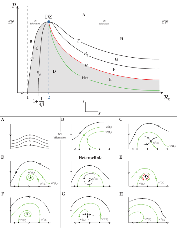
Figure 2. DZ bifurcation diagram associated to (4). In the regions C, D and E, the disease persists in the population. Compare with numerics of Figure 5.

4.2. Proof of Theorem A and the structure of the article

The jacobian matrix of the vector field associated to (4) at $E_{2}^{p}$ when $(\mathcal{R}_{0}^{\star},p^{\star})=\left(2,\frac{A^{2}}{4m}\right)$ is given by:

$$\left(\begin{array}[]{cc}\dfrac{p^{\star}m\beta^{2}-\left(\sigma+g\right)^{2}}{\beta\left(\sigma+g\right)}&-\left(\sigma+g\right)\\ \\ \dfrac{-p^{\star}m\beta^{2}+A\left(\sigma+g\right)\beta-\left(\sigma+g\right)^{2}}{\beta\left(\sigma+g\right)}&0\end{array}\right)$$ (9)

$$= \left(\begin{array}[]{cc}\dfrac{p^{\star}m}{A}\mathcal{R}_{0}^{\star}-\dfrac{A}{\mathcal{R}_{0}^{\star}}&-\left(\sigma+g\right)\\ \\ -\dfrac{p^{\star}m}{A}\mathcal{R}_{0}^{\star}+A-\dfrac{A}{\mathcal{R}_{0}^{\star}}&0\end{array}\right)$$ (13)

$$= \left(\begin{array}[]{cc}0&-\left(\sigma+g\right)\\ \\ 0&0\end{array}\right).$$ (17)

It is easy to verify that the matrix (17) is non-hyperbolic and has a double zero eigenvalue. This is why we say that, for $(\mathcal{R}_{0}^{\star},p^{\star})=\left(2,\frac{A^{2}}{4m}\right)$, the point $E_{2}^{p}$ is a singularity of codimension 2. The associated DZ bifurcations exist if the vector field $f_{(\mathcal{R}_{0},p)}$, at the bifurcation point, satisfies the nondegeneracy conditions described in [25, pp. 316–322]. Instead of verifying these additional conditions, we check analytically the existence of all bifurcation curves that pass through the point $(\mathcal{R}_{0}^{\star},p^{\star})=\left(2,\frac{A^{2}}{4m}\right)$, as pointed out in Table 1.

Bifurcation/Transition	Curve in Figure 2	Section
Saddle-node	$SN$	6.2
Transcritical	$T$	6.3
Belyakov	$B_{t}$	6.4
Hopf	$H$	6.5
Heteroclinic	Het.	6.6

Table 1. Codimension 1 bifurcations that characterizes the DZ bifurcation and structure of the proof of Theorem A.

For the sake of completeness, we have added in Section 5 a study of model (4) for $p=0$. The curve representing the heteroclinic cycle, denoted by $\mathcal{H}$, in the space of parameters $(\mathcal{R}_{0},p)$ was obtained by interpolation. The estimated correlation between the two parameters where one observes a repelling heteroclinic cycle is $1$ (precision: $10^{-5}$), as the reader may check in Section 6.6 and Appendix A. We simulate the dynamics in all hyperbolic regions associated to the DZ singularity in Figure 5. Section 8 finishes this article.

4.3. Biological consequences

As a direct consequence of Theorem A, we are able to locate three regions in the parameter space $(\mathcal{R}_{0},p)$ where the disease persists (C, D and E), i.e. there is a set with positive Lebesgue measure (in the phase space) whose $\omega$-limit is the endemic equilibrium. In regions C and D, trajectories starting “below” $W^{s}(E_{0}^{p})$ tend to $E_{2}^{p}$. In region E, there is a repelling periodic solution $\mathcal{C}$ (arising from the Hopf bifurcation) which is responsible for the maintenance of an endemic region where the disease persists.

In region E, if we assume seasonality in the transmission rate $\beta$, the associated flow exhibits a strange repeller and hyperbolic horseshoes, as a consequence of the works [9, 41]. The heteroclinic cycle $\mathcal{H}$ is a repeller. In the regions F, G and H, the high vaccination does not play a major role in the elimination of the disease because the carrying capacity $A$ is small compared with the number of Infected individuals that are being generated.

5. The case without vaccination $(p=0)$

For the sake of completeness, we analyze model (4) considering $p=0$:

$$\dot{x}=f_{(\mathcal{R}_{0},0)}(x)\quad\Leftrightarrow\quad\begin{cases}&\dot{S}=S(A-S)-\beta IS\\ \\ &\dot{I}=\beta IS-\left(\sigma+g\right)I.\end{cases}$$ (18)

The disease-free equilibria of system (18) are obtained by imposing $I=0$. Then we get:

$$E_{0}\equiv E_{0}^{0}=\left(0,0\right)\quad\text{and}\quad E_{1}\equiv E_{1}^{0}=\left(A,0\right).$$

With respect to the endemic equilibrium, we know that:

$$E_{2}=\left(\dfrac{\sigma+g}{\beta},\dfrac{A\beta-\left(\sigma+g\right)}{\beta^{2}}\right)\overset{\eqref{R0}}{=}\left(\dfrac{A}{\mathcal{R}_{0}},\dfrac{A}{\beta}\left(1-\dfrac{1}{\mathcal{R}_{0}}\right)\right).$$

The formal equilibrium $E_{2}\equiv E_{2}^{0}$ lies in the interior of the first quadrant when $\mathcal{R}_{0}>1$.

The jacobian matrix of the vector field associated to (18) at a general point $E=(S,I)\in(\mathbb{R}_{0}^{+})^{2}$ is given by:

$$\begin{array}[]{lcl}J(E)=\left(\begin{array}[]{cc}-\beta I+A-2S&-\beta S\\ \\ \beta I&\beta S-\left(\sigma+g\right)\end{array}\right)\end{array}.$$ (19)

Evaluating $J(E)$ at $E_{0}$, $E_{1}$ and $E_{2}$ we have:

$$J(E_{0})=\left(\begin{array}[]{cc}A&0\\ \\ 0&-\left(\sigma+g\right)\end{array}\right)\qquad J(E_{1})=\left(\begin{array}[]{cc}-A&-A\beta\\ \\ 0&A\beta-\left(\sigma+g\right)\end{array}\right).$$

and

$$J(E_{2})=\left(\begin{array}[]{cc}-\dfrac{\sigma+g}{\beta}&-\left(\sigma+g\right)\\ \\ \dfrac{A\beta-\left(\sigma+g\right)}{\beta}&0\end{array}\right),$$

respectively.

Lemma 2.

System (18) exhibits:

1. two disease-free equilibria, $E_{0}$ and  $E_{1}$, such that:

   1. for all $\mathcal{R}_{0}\in\mathbb{R}^{+}$, $E_{0}$ is a saddle;

   2. if  $\mathcal{R}_{0}<1$, then  $E_{1}$ is a sink. If  $\mathcal{R}_{0}>1$, then  $E_{1}$ is a saddle;

   3. at  $\mathcal{R}_{0}=1$,  $E_{1}$ undergoes a transcritical bifurcation with $E_{2}$.
      

2. an endemic equilibrium $E_{2}$ such that:
   

   1. if  $1<\mathcal{R}_{0}<1+\frac{1}{4\beta}$, then  $E_{2}$ is a stable node;

   2. if  $\mathcal{R}_{0}>1+\frac{1}{4\beta}$, then  $E_{2}$ is a stable focus;

   3. at  $\mathcal{R}_{0}=1+\frac{1}{4\beta}$,  $E_{2}$ undergoes a Belyakov transition.
      

Proof.

1. The eigenvalues of $J(E_{0})$ are  $-\left(\sigma+g\right)<0$ and $A>0$. Since the eigenvalues of $J(E_{0})$ have real part with opposite signs, then $E_{0}$ is a saddle for all $\mathcal{R}_{0}\in\mathbb{R}^{+}$. The eigenvalues of $J(E_{1})$ are $A\beta-\left(\sigma+g\right)$ and $-A<0$. If

   $$A\beta-\left(\sigma+g\right)<0\quad\Leftrightarrow\quad\dfrac{A\beta}{\sigma+g}<1\quad\overset{\eqref{R0}}{\Leftrightarrow}\quad\mathcal{R}_{0}<1,$$

   then $E_{1}$ is a sink. If  $\mathcal{R}_{0}>1$, then $E_{1}$ is a saddle. Therefore, in the vertical direction, $E_{1}$ interchanges its stability with $E_{2}$ from stable to unstable at $\mathcal{R}_{0}=1$ (transcritical bifurcation).
   

2. The eigenvalues of $J(E_{2})$ are given by:

   $$\lambda_{1}\coloneqq\dfrac{-\left(\sigma+g\right)-\sqrt{\Delta}}{2\beta}\qquad\text{and}\qquad\lambda_{2}\coloneqq\dfrac{-\left(\sigma+g\right)+\sqrt{\Delta}}{2\beta},$$

   where $\Delta=-4\left(\sigma+g\right)\left[\left(-\beta-\dfrac{1}{4}\right)g+A\beta^{2}-\sigma\beta-\dfrac{\sigma}{4}\right]$. Since $\beta>0$ and $\sigma+g>0$, it is easy to verify that $\lambda_{1}$ has negative real part. The eigenvalue $\lambda_{2}$ has negative real part if and only if

   $$-\left(\sigma+g\right)+\sqrt{\Delta}<0$$

   $$\Leftrightarrow \sqrt{\Delta}<\sigma+g$$

   $$\Leftrightarrow \begin{cases}&\Delta\geq 0\\ \\ &\Delta<\left(\sigma+g\right)^{2}\end{cases}$$

   $$\Leftrightarrow \begin{cases}&-4\left(\sigma+g\right)\left[\left(-\beta-\dfrac{1}{4}\right)g+A\beta^{2}-\sigma\beta-\dfrac{\sigma}{4}\right]\geq 0\\ \\ &-4\left(\sigma+g\right)\left[\left(-\beta-\dfrac{1}{4}\right)g+A\beta^{2}-\sigma\beta-\dfrac{\sigma}{4}\right]<\left(\sigma+g\right)^{2}\end{cases}$$

   $$\Leftrightarrow \begin{cases}&\left(-\beta-\dfrac{1}{4}\right)g+A\beta^{2}-\sigma\beta-\dfrac{\sigma}{4}\leq 0\\ \\ &-4\left[\left(-\beta-\dfrac{1}{4}\right)g+A\beta^{2}-\sigma\beta-\dfrac{\sigma}{4}\right]<\sigma+g\end{cases}$$

   $$\Leftrightarrow \begin{cases}&4A\beta^{2}-\left(4\sigma\beta+\sigma\right)-\left(4\beta+1\right)g\leq 0\\ \\ &g-A\beta+\sigma<0\end{cases}$$

   $$\Leftrightarrow \begin{cases}&4\beta\mathcal{R}_{0}-\dfrac{\sigma\left(4\beta+1\right)}{\sigma+g}-\dfrac{g\left(4\beta+1\right)}{\sigma+g}\leq 0\\ \\ &\mathcal{R}_{0}>1\end{cases}$$

   $$\Leftrightarrow \begin{cases}&\mathcal{R}_{0}\leq 1+\dfrac{1}{4\beta}\\ \\ &\mathcal{R}_{0}>1.\end{cases}$$

   If $1<\mathcal{R}_{0}<1+\frac{1}{4\beta}$, then $\lambda_{2}<0$ and $E_{2}$ is a stable node. In an analogous way, if $\mathcal{R}_{0}>1+\frac{1}{4\beta}$, then $\Delta<0$ and $E_{2}$ is a stable focus. Hence, $E_{2}$ evolves from stable node to stable focus at $\mathcal{R}_{0}=1+\frac{1}{4\beta}$ (Belyakov transition).

∎

In Figure 3, one observes the scheme of the equilibria stability of system (18) for different values of $\mathcal{R}_{0}$. The transcritical bifurcation at $\mathcal{R}_{0}=1$ represents the threshold for the existence of the endemic disease in the population, agreeing well with the empirical belief.

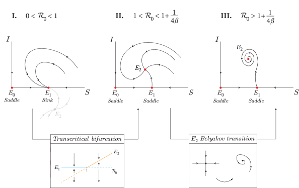
Figure 3. Phase diagram of (18) for different values of $\mathcal{R}_{0}$. I. $E_{1}$ is a global attractor when restricted to the closure of the first quadrant. II. Besides the $E_{0}$ and $E_{1}$, there exists a stable node $E_{2}$. III. Besides the $E_{0}$ and $E_{1}$, there exists a stable focus $E_{2}$. From I. to II. $E_{1}$ undergoes a transcritical bifurcation at $\mathcal{R}_{0}=1$. From II. to III. $E_{2}$ evolves a Belyakov transition at $\mathcal{R}_{0}=1+\frac{1}{4\beta}$.

6. The case with constant vaccination $(p>0)$

We analyze (4) by considering $p>0$ and $\mathcal{R}_{0}>1$ (see (C3)):

$$\dot{x}=f_{(\mathcal{R}_{0},0)}(x)\quad\Leftrightarrow\quad\begin{cases}&\dot{S}=S(A-S)-\beta IS-pm\\ \\ &\dot{I}=\beta IS-\left(\sigma+g\right)I.\end{cases}$$ (20)

For $A$ and $m$ fixed, we settle the following maps that will be used throughout this text:

$$p_{SN}(\mathcal{R}_{0})\coloneqq\dfrac{A^{2}}{4m}\quad\text{,}\quad p_{T}(\mathcal{R}_{0})\coloneqq\dfrac{A^{2}}{m}\dfrac{\left(\mathcal{R}_{0}-1\right)}{\mathcal{R}_{0}^{2}}\quad\text{and}\quad p_{H}(\mathcal{R}_{0})\coloneqq\dfrac{A^{2}}{m\mathcal{R}_{0}^{2}},$$ (21)

for $\mathcal{R}_{0}>1$. It is easy to verify that:

• $p_{SN}$ is a constant map and
  

• if $1<\mathcal{R}_{0}<2$, then $p_{H}(\mathcal{R}_{0})>p_{SN}(\mathcal{R}_{0})$, which does not make sense (because $E_{2}^{p}$ does not exist in the first quadrant as a consequence of Lemmas 3 and 5). This is the reason why we consider the set $[2,+\infty[$ as the domain of $p_{H}$.
  

6.1. Preparatory section

We state a preliminary result that will be used in the sequel.

Lemma 3.

The following statements hold for the maps given in (21):

1. If  $\mathcal{R}_{0}>1$ and  $\mathcal{R}_{0}\neq 2$, then  $p_{T}(\mathcal{R}_{0})<p_{SN}(\mathcal{R}_{0})$;

2. $p_{H}(2)=p_{T}(2)=p_{SN}(2)$;

3. If  $\mathcal{R}_{0}>2$, then  $p_{H}(\mathcal{R}_{0})<p_{T}(\mathcal{R}_{0})<p_{SN}(\mathcal{R}_{0})$.
   

Proof.

1. From (21), it follows that:

   $$p_{T}(\mathcal{R}_{0})<p_{SN}(\mathcal{R}_{0})$$

   $$\Leftrightarrow \dfrac{A^{2}}{m}\dfrac{\left(\mathcal{R}_{0}-1\right)}{\mathcal{R}_{0}^{2}}<\dfrac{A^{2}}{4m}$$

   $$\Leftrightarrow \dfrac{\mathcal{R}_{0}-1}{\mathcal{R}_{0}^{2}}<\dfrac{1}{4}$$

   $$\Leftrightarrow \mathcal{R}_{0}^{2}-4\mathcal{R}_{0}+4>0$$

   $$\Leftrightarrow (\mathcal{R}_{0}-2)^{2}>0.$$

2. This item follows if we evaluate $p_{H}$, $p_{T}$ and $p_{SN}$ at $\mathcal{R}_{0}=2$.
   

3. From (21), we have:

   $$p_{H}(\mathcal{R}_{0})<p_{T}(\mathcal{R}_{0})$$

   $$\Leftrightarrow \dfrac{A^{2}}{m\mathcal{R}_{0}^{2}}<\dfrac{A^{2}}{m}\dfrac{\left(\mathcal{R}_{0}-1\right)}{\mathcal{R}_{0}^{2}}$$

   $$\Leftrightarrow \mathcal{R}_{0}-1>1$$

   $$\Leftrightarrow \mathcal{R}_{0}>2.$$

   The remaining inequality follows from the previous item and transitivity.

∎

6.2. Saddle-node bifurcation

The general jacobian matrix of (20) at $E^{p}=(S^{p},I^{p})\in(\mathbb{R}_{0}^{+})^{2}$ coincides with that of (19). At $E_{0}^{p}$, $E_{1}^{p}$ and $E_{2}^{p}$, the matrix (19) takes the form:

$$J(E_{0}^{p})=\left(\begin{array}[]{cc}A-2S_{0}^{p}&-\beta S_{0}^{p}\\ \\ 0&\beta S_{0}^{p}-\left(\sigma+g\right)\end{array}\right),\qquad J(E_{1}^{p})=\left(\begin{array}[]{cc}A-2S_{1}^{p}&-\beta S_{1}^{p}\\ \\ 0&\beta S_{1}^{p}-\left(\sigma+g\right)\end{array}\right)$$

and

$$J(E_{2}^{p})=\left(\begin{array}[]{cc}\dfrac{pm\beta^{2}-\left(\sigma+g\right)^{2}}{\beta\left(\sigma+g\right)}&-\left(\sigma+g\right)\\ \\ \dfrac{-pm\beta^{2}+A\left(\sigma+g\right)\beta-\left(\sigma+g\right)^{2}}{\beta\left(\sigma+g\right)}&0\end{array}\right),$$ (27)

respectively.

Lemma 4.

The following statements hold for model (20):

1. If  $p>p_{SN}(\mathcal{R}_{0})$, then $E_{0}^{p}$ and $E_{1}^{p}$ do not exist in the first quadrant of $(S,I)$.
   

2. If  $p_{T}(\mathcal{R}_{0})<p<p_{SN}(\mathcal{R}_{0})$, then:

   1. $E_{0}^{p}$ is a saddle and $E_{1}^{p}$ is a sink for  $1<\mathcal{R}_{0}<2$;

   2. $E_{0}^{p}$ is a source and $E_{1}^{p}$ is a saddle for  $\mathcal{R}_{0}>2$.
      

3. If  $p<p_{T}(\mathcal{R}_{0})$ and  $\mathcal{R}_{0}>1$, then  $E_{0}^{p}$ and  $E_{1}^{p}$ are saddles.
   

Proof.

The eigenvalues of $J(E_{0}^{p})$ are $A-2S_{0}^{p}$ and $\beta S_{0}^{p}-(\sigma+g)$. We know that

$$A-2S_{0}^{p}>0$$

$$\Leftrightarrow \displaystyle\dfrac{2A-2A+2\sqrt{A^{2}-4pm}}{2}>0$$

$$\Leftrightarrow \displaystyle\sqrt{A^{2}-4pm}>0\quad\text{if $p\leq p_{SN}(\mathcal{R}_{0})$}$$

1. If $p>p_{SN}(\mathcal{R}_{0})$, then $E_{0}^{p}$ and $E_{1}^{p}$ do not exist.
   

2. We may write:

   $$\beta S_{0}^{p}-(\sigma+g)<0$$ (28)

   $$\Leftrightarrow S_{0}^{p}<\dfrac{\sigma+g}{\beta}$$

   $$\overset{\eqref{S0_ref}}{\Leftrightarrow} \displaystyle\dfrac{A-\sqrt{A^{2}-4pm}}{2}<\dfrac{\sigma+g}{\beta}$$

   $$\Leftrightarrow \displaystyle\sqrt{A^{2}-4pm}>A-\dfrac{2\left(\sigma+g\right)}{\beta}$$

   $$\Leftrightarrow \displaystyle\sqrt{A^{2}-4pm}>\dfrac{A\mathcal{R}_{0}}{\mathcal{R}_{0}}-\dfrac{2A}{\mathcal{R}_{0}}$$

   $$\Leftrightarrow \displaystyle\sqrt{A^{2}-4pm}>\dfrac{A\left(\mathcal{R}_{0}-2\right)}{\mathcal{R}_{0}}$$

   $$\Leftrightarrow \begin{cases}&A^{2}-4pm\geq 0\quad,\qquad 1<\mathcal{R}_{0}<2\\ \\ &A^{2}-4pm>\dfrac{A^{2}\left(\mathcal{R}_{0}-2\right)^{2}}{\mathcal{R}_{0}^{2}}\quad,\qquad\mathcal{R}_{0}\geq 2\end{cases}$$

   $$\overset{\eqref{pes_eq}}{\Leftrightarrow} \begin{cases}&p\leq p_{SN}\quad,\qquad 1<\mathcal{R}_{0}<2\\ \\ &p<\dfrac{A^{2}\left(\mathcal{R}_{0}-1\right)}{m\mathcal{R}_{0}^{2}}\quad,\qquad\mathcal{R}_{0}\geq 2\end{cases}$$

   $$\overset{\eqref{pes_eq}}{\Rightarrow} \begin{cases}&p<p_{SN}(\mathcal{R}_{0})\quad,\qquad 1<\mathcal{R}_{0}<2\\ \\ &p<p_{T}(\mathcal{R}_{0})\quad,\qquad\mathcal{R}_{0}>2\end{cases},$$

   then the eigenvalues of $J(E_{0}^{p})$ have real part with opposite signs and $E_{0}^{p}$ is a saddle. On the other hand, if

   $$\beta S_{0}-(\sigma+g)>0$$ (29)

   $$\Leftrightarrow S_{0}>\dfrac{\sigma+g}{\beta}$$

   $$\Leftrightarrow \sqrt{A^{2}-4pm}<\dfrac{A\left(\mathcal{R}_{0}-2\right)}{\mathcal{R}_{0}}$$

   $$\Leftrightarrow 0\leq A^{2}-4pm<\dfrac{A^{2}\left(\mathcal{R}_{0}-2\right)^{2}}{\mathcal{R}_{0}^{2}}\quad,\qquad\mathcal{R}_{0}>2$$

   $$\overset{\eqref{pes_eq}}{\Rightarrow} p_{T}(\mathcal{R}_{0})<p<p_{SN}(\mathcal{R}_{0})\quad,\qquad\mathcal{R}_{0}>2,$$

   then the eigenvalues of $J(E_{0}^{p})$ have real part with positive signs, and $E_{0}^{p}$ is a source. Moreover, the eigenvalues of $J(E_{1}^{p})$ are $A-2S_{1}^{p}<0$ and $\beta S_{1}^{p}-\left(\sigma+g\right)$. Hence, if

   $$\beta S_{1}^{p}-(\sigma+g)<0$$ (30)

   $$\Leftrightarrow S_{1}^{p}<\dfrac{\sigma+g}{\beta}$$

   $$\Leftrightarrow \sqrt{A^{2}-4pm}<\dfrac{A\left(2-\mathcal{R}_{0}\right)}{\mathcal{R}_{0}}$$

   $$\Leftrightarrow 0\leq A^{2}-4pm<\dfrac{A^{2}\left(2-\mathcal{R}_{0}\right)^{2}}{\mathcal{R}_{0}^{2}}\quad,\qquad 1<\mathcal{R}_{0}<2$$

   $$\overset{\eqref{pes_eq}}{\Rightarrow} p_{T}(\mathcal{R}_{0})<p<p_{SN}(\mathcal{R}_{0})\quad,\qquad 1<\mathcal{R}_{0}<2,$$

   then both eigenvalues of $J(E_{1}^{p})$ have negative real part and $E_{1}^{p}$ is a sink. If

   $$\beta S_{1}^{p}-(\sigma+g)>0$$ (31)

   $$\Leftrightarrow S_{1}^{p}>\dfrac{\sigma+g}{\beta}$$

   $$\Leftrightarrow \sqrt{A^{2}-4pm}>\dfrac{A\left(2-\mathcal{R}_{0}\right)}{\mathcal{R}_{0}}$$

   $$\Leftrightarrow \begin{cases}&A^{2}-4pm>\dfrac{A^{2}\left(2-\mathcal{R}_{0}\right)^{2}}{\mathcal{R}_{0}^{2}}\quad,\qquad 1<\mathcal{R}_{0}\leq 2\\ \\ &A^{2}-4pm\geq 0\quad,\qquad\mathcal{R}_{0}>2\end{cases}$$

   $$\Leftrightarrow \begin{cases}&p<\dfrac{A^{2}}{m}\left(\dfrac{\mathcal{R}_{0}-1}{\mathcal{R}_{0}^{2}}\right)\quad,\qquad 1<\mathcal{R}_{0}\leq 2\\ \\ &p\leq\dfrac{A^{2}}{4m}\quad,\qquad\mathcal{R}_{0}>2\end{cases}$$

   $$\overset{\eqref{pes_eq}}{\Rightarrow} \begin{cases}&p<p_{T}(\mathcal{R}_{0})\quad,\qquad 1<\mathcal{R}_{0}<2\\ \\ &p<p_{SN}(\mathcal{R}_{0})\quad,\qquad\mathcal{R}_{0}>2,\end{cases}$$

   then the eigenvalues of $J(E_{1}^{p})$ have real part with opposite signs and $E_{1}^{p}$ is a saddle. Therefore, from (28) and (30), we conclude that:
   

   1. if  $p_{T}(\mathcal{R}_{0})<p<p_{SN}(\mathcal{R}_{0})$ and  $1<\mathcal{R}_{0}<2$, then $E_{0}^{p}$ is a saddle and $E_{1}^{p}$ is a sink;
      

   2. if  $p_{T}(\mathcal{R}_{0})<p<p_{SN}(\mathcal{R}_{0})$, then $E_{0}^{p}$ is a source and $E_{1}^{p}$ is a saddle, for  $\mathcal{R}_{0}>2$, under conditions (29) and (31).
      

3. From (28) and (31), we conclude that if  $p<p_{T}(\mathcal{R}_{0})$, then $E_{0}^{p}$ and $E_{1}^{p}$ are saddles.

∎

6.3. Transcritical bifurcation

Lemma 5.

The endemic equilibrium $E_{2}^{p}$ undergoes a transcritical bifurcation at $p=p_{T}(\mathcal{R}_{0})$ and lies in the interior of the first quadrant if  $p<p_{T}(\mathcal{R}_{0})$.

Proof.

The equilibrium $E_{2}^{p}$ lies in the interior of the first quadrant if both $S_{2}^{p}$ and $I_{2}^{p}$ are positive. It is clear that $S_{2}^{p}=\dfrac{\sigma+g}{\beta}>0$. Since $\beta^{2}(\sigma+g)>0$, we have

$$I_{2}^{p}>0\quad\Leftrightarrow\quad-pm\beta^{2}+A\left(\sigma+g\right)\beta-\left(\sigma+g\right)^{2}>0.$$

Solving the previous inequality in order to $p$, one gets:

$$-pm\beta^{2}+A\left(\sigma+g\right)\beta-\left(\sigma+g\right)^{2}>0$$

$$\Leftrightarrow p<\dfrac{A\left(\sigma+g\right)\beta-\left(\sigma+g\right)^{2}}{m\beta^{2}}$$

$$\Leftrightarrow p<\dfrac{A\left(\sigma+g\right)^{2}\beta}{m\left(\sigma+g\right)\beta^{2}}-\dfrac{\left(\sigma+g\right)^{2}A^{2}}{A^{2}m\beta^{2}}$$

$$\Leftrightarrow p<\dfrac{\left(\sigma+g\right)^{2}A^{2}}{m\beta^{2}A^{2}}\mathcal{R}_{0}-\dfrac{1}{\mathcal{R}_{0}^{2}}\dfrac{A^{2}}{m}$$

$$\Leftrightarrow p<\dfrac{1}{\mathcal{R}_{0}}\dfrac{A^{2}}{m}-\dfrac{1}{\mathcal{R}_{0}^{2}}\dfrac{A^{2}}{m}$$

$$\Leftrightarrow p<\dfrac{A^{2}}{m}\dfrac{\left(\mathcal{R}_{0}-1\right)}{\mathcal{R}_{0}^{2}}$$

$$\overset{\eqref{pes_eq}}{\Leftrightarrow} p<p_{T}(\mathcal{R}_{0})$$

since $\mathcal{R}_{0}>1$. Hence, $E_{2}^{p}$ undergoes a trancritical bifurcation along the line $p=p_{T}(\mathcal{R}_{0})$ and interchanges its stability with $E_{2}^{p}$ (if $\mathcal{R}_{0}<2$) and $E_{1}^{p}$ (if $\mathcal{R}_{0}>2$). ∎

6.4. Belyakov transition

We settle the following functions that will be used throughout this text:

$$\Delta_{2}(p) \coloneqq m^{2}p^{2}\beta^{4}+4pm\left(\sigma+g\right)^{2}\beta^{3}-\left[4A\left(\sigma+g\right)+2pm\right]\left(\sigma+g\right)^{2}\beta^{2}$$ (32)

$$+4\left(\sigma+g\right)^{4}\beta+\left(\sigma+g\right)^{4}$$

$$= m^{2}\beta^{4}p^{2}+2m\beta^{2}\left(2\beta-1\right)\left(\sigma+g\right)^{2}p+\left(4\beta+1\right)\left(\sigma+g\right)^{4}$$

$$-4A\left(\sigma+g\right)^{3}\beta^{2},$$

$$p_{B_{t}}^{(1)}\left(\mathcal{R}_{0}\right) \coloneqq \dfrac{\left(-2\beta+1-2\displaystyle\sqrt{\beta\left(\mathcal{R}_{0}+\beta-2\right)}\right)A^{2}}{m\mathcal{R}_{0}^{2}},$$ (33)

$$p_{B_{t}}^{(2)}\left(\mathcal{R}_{0}\right) \coloneqq \dfrac{\left(-2\beta+1+2\displaystyle\sqrt{\beta\left(\mathcal{R}_{0}+\beta-2\right)}\right)A^{2}}{m\mathcal{R}_{0}^{2}},$$ (34)

for  $\beta\left(\mathcal{R}_{0}+\beta-2\right)>0\Leftrightarrow\beta>2-\mathcal{R}_{0}$, where  $p_{B_{t}}^{(1)}(\mathcal{R}_{0})$ and  $p_{B_{t}}^{(2)}(\mathcal{R}_{0})$ are the square roots of  $\Delta_{2}(p)$ written as function of $\mathcal{R}_{0}$. It is easy to verify that  $p_{B_{t}}^{(1)}(\mathcal{R}_{0})<p_{B_{t}}^{(2)}(\mathcal{R}_{0})$.

Lemma 6.

If  $\beta\geq\frac{1}{2}$ and  $\mathcal{R}_{0}>1+\frac{1}{4\beta}$, then  $p_{B_{t}}^{(2)}(\mathcal{R}_{0})>0$.

Proof.

From (34) we know that if

$$\dfrac{\left(-2\beta+1+2\displaystyle\sqrt{\beta\left(\mathcal{R}_{0}+\beta-2\right)}\right)A^{2}}{m\mathcal{R}_{0}^{2}}>0$$

$$\Leftrightarrow \left(-2\beta+1+2\displaystyle\sqrt{\beta\left(\mathcal{R}_{0}+\beta-2\right)}\right)A^{2}>0$$

$$\Leftrightarrow 2\displaystyle\sqrt{\beta\left(\mathcal{R}_{0}+\beta-2\right)}>2\beta-1$$

$$\Leftrightarrow \displaystyle\sqrt{\beta\left(\mathcal{R}_{0}+\beta-2\right)}>\beta-\dfrac{1}{2}$$

$$\Leftrightarrow \begin{cases}&\beta-\dfrac{1}{2}\geq 0\quad,\qquad\beta\left(\mathcal{R}_{0}+\beta-2\right)>\left[\beta-\dfrac{1}{2}\right]^{2}\\ \\ &\beta-\dfrac{1}{2}<0\quad,\qquad\beta\left(\mathcal{R}_{0}+\beta-2\right)\geq 0\end{cases}$$

$$\Leftrightarrow \begin{cases}&\beta\geq\dfrac{1}{2}\quad,\qquad\beta\mathcal{R}_{0}-2\beta>-\beta+\dfrac{1}{4}\\ \\ &\beta<\dfrac{1}{2}\quad,\qquad\beta^{2}+\mathcal{R}_{0}\beta-2\beta\geq 0\end{cases}$$

$$\Leftrightarrow \begin{cases}&\beta\geq\dfrac{1}{2}\quad,\qquad\beta\left(\mathcal{R}_{0}-1\right)>\dfrac{1}{4}\\ \\ &\beta<\dfrac{1}{2}\quad,\qquad\beta\geq 2-\mathcal{R}_{0}\end{cases}$$

$$\Leftrightarrow \begin{cases}&\beta\geq\dfrac{1}{2}\quad,\qquad\mathcal{R}_{0}>1+\dfrac{1}{4\beta}\\ \\ &\beta<\dfrac{1}{2}\quad,\qquad\mathcal{R}_{0}\geq 2-\beta\end{cases},$$

then $p_{B_{t}}^{(2)}(\mathcal{R}_{0})>0$. If  $\mathcal{R}_{0}=1+\frac{1}{4\beta}$, then  $p_{B_{t}}^{(2)}(\mathcal{R}_{0})=0$ and if  $\mathcal{R}_{0}=2$, then  $p_{B_{t}}^{(2)}(\mathcal{R}_{0})=p_{SN}(\mathcal{R}_{0})$. Hence we conclude that if  $\beta\geq\frac{1}{2}$ and $\mathcal{R}_{0}>1+\frac{1}{4\beta}$, then  $p_{B_{t}}^{(2)}(\mathcal{R}_{0})>0$. ∎

Before we analyze the stability of $E_{2}^{p}$, we remind the readers that $E_{2}^{p}$ exists in the first quadrant when $p<p_{T}(\mathcal{R}_{0})$ (by Lemma 5).

Lemma 7.

The following statements hold for model (20):

1. If  $p_{B_{t}}^{(2)}(\mathcal{R}_{0})<p<p_{T}(\mathcal{R}_{0})$, then  $\Delta_{2}(p)>0$ and $E_{2}^{p}$ is:

   
   

   1. stable node for  $\mathcal{R}_{0}<2$;

   2. unstable node for  $p>p_{H}(\mathcal{R}_{0})$.

   
   

2. If  $p<p_{B_{t}}^{(2)}(\mathcal{R}_{0})$, then  $\Delta_{2}(p)<0$ and  $E_{2}^{p}$ is:

   
   

   1. stable focus for  $p<p_{H}(\mathcal{R}_{0})$;

   2. unstable focus for  $p>p_{H}(\mathcal{R}_{0})$.

Hence, $E_{2}^{p}$ undergoes a Belyakov transition at  $p=p_{B_{t}}^{(2)}(\mathcal{R}_{0})$.

Proof.

1. With respect to (20), the eigenvalues of the jacobian matrix of $J(E_{2}^{p})$ are:

   $$\lambda_{1}=\dfrac{pm\beta^{2}-\left(\sigma+g\right)^{2}-\displaystyle\sqrt{\Delta_{2}(p)}}{2\beta\left(\sigma+g\right)}\qquad\text{and}\qquad\lambda_{2}=\dfrac{pm\beta^{2}-\left(\sigma+g\right)^{2}+\displaystyle\sqrt{\Delta_{2}(p)}}{2\beta\left(\sigma+g\right)}.$$

   where $\lambda_{1}<\lambda_{2}$. Hence, if $\lambda_{1}>0$, then $\lambda_{2}>0$. If $\lambda_{2}<0$, then $\lambda_{1}<0$. We know from (32), (33), (34) and Lemma 6 that:

   $$\begin{cases}\,\,\Delta_{2}>0\,\,,\qquad\text{if}\quad\,0<p<p_{B_{t}}^{(1)}$ or \,$p_{B_{t}}^{(2)}<p<+\infty\\ \\ \,\,\Delta_{2}<0\,\,,\qquad\text{if}\quad\,p_{B_{t}}^{(1)}<p<p_{B_{t}}^{(2)}\end{cases},$$

   where $p_{B_{t}}^{(2)}(\mathcal{R}_{0})<p_{T}(\mathcal{R}_{0})$.

   
   

   (1) Therefore, if

   $$\lambda_{1}>0$$

   $$\Leftrightarrow \dfrac{pm\beta^{2}-\left(\sigma+g\right)^{2}-\displaystyle\sqrt{\Delta_{2}(p)}}{2\beta\left(\sigma+g\right)}>0$$

   $$\Leftrightarrow \displaystyle\sqrt{\Delta_{2}(p)}<pm\beta^{2}-\left(\sigma+g\right)^{2}$$

   $$\Leftrightarrow \begin{cases}&\Delta_{2}(p)\geq 0\\ \\ &\Delta_{2}(p)<\left[pm\beta^{2}-\left(\sigma+g\right)^{2}\right]^{2}\end{cases}\qquad,\quad pm\beta^{2}-\left(\sigma+g\right)^{2}>0$$

   $$\Leftrightarrow \begin{cases}&p\geq p_{B_{t}}^{(2)}(\mathcal{R}_{0})\\ \\ &p<p_{T}(\mathcal{R}_{0})\end{cases}\qquad,\quad p>p_{H}(\mathcal{R}_{0})$$

   $$\Rightarrow p_{B_{t}}^{(2)}(\mathcal{R}_{0})<p<p_{T}(\mathcal{R}_{0})\quad,\qquad\text{for}\quad p>p_{H}(\mathcal{R}_{0})$$

   then $\lambda_{1}>0\Rightarrow\lambda_{2}>0$ and $E_{2}^{p}$ is an unstable node. Analogously, we proceed in the same way for $\lambda_{2}<0$. If

   $$\lambda_{2}<0$$

   $$\Leftrightarrow \dfrac{pm\beta^{2}-\left(\sigma+g\right)^{2}+\displaystyle\sqrt{\Delta_{2}(p)}}{2\beta\left(\sigma+g\right)}<0$$

   $$\Leftrightarrow \displaystyle\sqrt{\Delta_{2}(p)}<\left(\sigma+g\right)^{2}-pm\beta^{2}$$

   $$\Leftrightarrow \begin{cases}&\Delta_{2}(p)\geq 0\\ \\ &\Delta_{2}(p)<\left[\left(\sigma+g\right)^{2}-pm\beta^{2}\right]^{2}\end{cases}\qquad,\quad\left(\sigma+g\right)^{2}-pm\beta^{2}>0$$

   $$\Leftrightarrow \begin{cases}&p\geq p_{B_{t}}^{(2)}(\mathcal{R}_{0})\\ \\ &p<p_{T}(\mathcal{R}_{0})\end{cases}\qquad,\quad p<p_{H}(\mathcal{R}_{0})$$

   $$\Rightarrow p_{B_{t}}^{(2)}(\mathcal{R}_{0})<p<p_{T}(\mathcal{R}_{0})\quad,\qquad\text{for}\quad p<p_{H}(\mathcal{R}_{0})$$

   then $\lambda_{2}<0\Rightarrow\lambda_{1}<0$ and $E_{2}^{p}$ is a stable node.

   
   

   (2) Now, let us assume that  $\Delta_{2}(p)<0$, which means that  $p<p_{B_{t}}^{(2)}(\mathcal{R}_{0})$, the eigenvalues are complex and  $E_{2}^{p}$ is a focus. If the real part of the eigenvalues of  $J(E_{2}^{p})$ is negative (and  $\beta$ is positive), i.e. if

   $$pm\beta^{2}-\left(\sigma+g\right)^{2}<0$$

   $$\Leftrightarrow pm\beta^{2}<\left(\sigma+g\right)^{2}$$

   $$\Leftrightarrow p<\dfrac{\left(\sigma+g\right)^{2}}{m\beta^{2}}$$

   $$\Leftrightarrow p<\dfrac{A^{2}}{m\mathcal{R}_{0}^{2}}$$

   $$\overset{\eqref{pes_eq}}{\Leftrightarrow} p<p_{H}(\mathcal{R}_{0}),$$

   then  $E_{2}^{p}$ is a stable focus. Otherwise  $E_{2}^{p}$ is an unstable focus. Also, we conclude that  $E_{2}^{p}$ undergoes a Belyakov transition at  $p=p_{B_{t}}^{(2)}(\mathcal{R}_{0})$, since $E_{2}^{p}$ changes its stability from a node to a focus.

∎

6.5. Hopf bifurcation

In this section we will find a line in the parameter space $(p,\mathcal{R}_{0})$ where a Hopf bifurcation occurs.

Lemma 8.

If  $p=p_{H}(\mathcal{R}_{0})$, then $E_{2}^{p}$ undergoes a subcritical Hopf bifurcation associated to an unstable periodic solution $\mathcal{C}$ (as $\mathcal{R}_{0}$ increases).

Figure 4. Phase portraits of system (20) when $E_{2}^{p}$ undergoes a subcritical Hopf bifurcation as $\mathcal{R}_{0}$ increases.

Proof.

Let the eigenvalues of $J(E_{2}^{p})$ given by

$$\lambda_{1}=\dfrac{pm\beta^{2}-\left(\sigma+g\right)^{2}-\displaystyle\sqrt{\Delta_{2}(p)}}{2\beta\left(\sigma+g\right)}\qquad\text{and}\qquad\lambda_{2}=\dfrac{pm\beta^{2}-\left(\sigma+g\right)^{2}+\displaystyle\sqrt{\Delta_{2}(p)}}{2\beta\left(\sigma+g\right)}.$$

From [42, pp. 151–153, Theorem 3.4.2 (adapted)] we know that the Hopf bifurcation occurs when the following conditions hold:

1. the eigenvalues of the map $Df(E_{2}^{p})$ (see (27)) have the form $\pm i\omega$ ($\omega>0$), which is equivalent to $\mathrm{Tr}\,J(E_{2}^{p})=0$, where $\mathrm{Tr}$ represents the usual trace operator. Indeed,

   $$\mathrm{Tr}\,J(E_{2}^{p})=0$$

   $$\Leftrightarrow \dfrac{pm\beta^{2}-\left(\sigma+g\right)^{2}}{\beta\left(\sigma+g\right)}=0$$

   $$\Leftrightarrow pm\beta^{2}-\left(\sigma+g\right)^{2}=0$$

   $$\Leftrightarrow p=\dfrac{\left(\sigma+g\right)^{2}}{m\beta^{2}}$$

   $$\Leftrightarrow p=\dfrac{A^{2}}{m\mathcal{R}_{0}^{2}}$$

   $$\overset{\eqref{pes_eq}}{\Leftrightarrow} p=p_{H}(\mathcal{R}_{0}).$$

   
   

2. $\dfrac{\mathrm{d}}{\mathrm{d}\mathcal{R}_{0}}\left(\operatorname{Re}\lambda_{j}(\mathcal{R}_{0})\right)\big{|}_{\mathcal{R}_{0}\in p_{H}}\neq 0$,  for $j\in\{1,2\}$:

   
   

   Hence, for $p=p_{H}(\mathcal{R}_{0})$ we get

   $$\dfrac{\mathrm{d}}{\mathrm{d}\mathcal{R}_{0}}\left(\operatorname{Re}\lambda_{j}(\mathcal{R}_{0})\right)\big{|}_{\mathcal{R}_{0}=\mathcal{R}_{0}^{\star}} = \dfrac{\mathrm{d}}{\mathrm{d}\mathcal{R}_{0}}\left(\dfrac{pm\beta^{2}}{2\beta\left(\sigma+g\right)}-\dfrac{\left(\sigma+g\right)^{2}}{2\beta\left(\sigma+g\right)}\right)\Big{|}_{\mathcal{R}_{0}=\mathcal{R}_{0}^{\star}}$$

   $$= \dfrac{\mathrm{d}}{\mathrm{d}\mathcal{R}_{0}}\left(\dfrac{\sigma+g}{2\beta}-\dfrac{A}{2\mathcal{R}_{0}}\right)\Big{|}_{\mathcal{R}_{0}=\mathcal{R}_{0}^{\star}}$$

   $$= \dfrac{A}{2{\mathcal{R}_{0}^{\star}}^{2}}\neq 0.$$

Hence, $E_{2}^{p}$ undergoes a subcritical Hopf bifurcation (as $\mathcal{R}_{0}$ increases; the periodic solution appears for $\mathcal{R}_{0}<\mathcal{R}_{0}^{\star}$ as illustrated in Figure 4. Figure 2 provides a better perspective of all bifurcations under consideration. ∎

6.6. Heteroclinic cycle

Finding explicitly a non-robust heteroclinic cycle (in the phase space) to two hyperbolic saddles and its bifurcating curve is a difficult task. In this section, we use polynomial interpolation (of rational degree) to find the latter curve. We proceed to explain the method that we have used to compute the map. All steps are described in Appendix A.

Using MATLAB_R2018a, we locate thirteen pairs $({\mathcal{R}_{0}}_{i},p_{i})$ in the parameter space $(\mathcal{R}_{0},p)$ where one observes a heteroclinic cycle associated to the disease-free equilibria $E_{0}^{p_{i}}$ and $E_{1}^{p_{i}}$ (see Table 2). The type of function for the interpolation should be appropriately chosen to fit the curve to our finite set of points [43, Part I, Section 1].

As suggested by [23], points in the parameter space that correspond to the heteroclinic cycle associated to the disease-free equilibria should lie on the graph of:

$$y=ax^{b}+c\quad\text{for}\quad a,b,c\in\mathbb{R}.$$

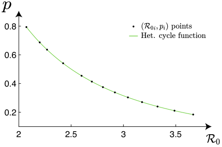
Figure 6. Function obtained by interpolation of 13 points (see Table 2) for which it is possible to observe the heteroclinic cycle in phase space $(S,I)$. The function obtained by interpolation for which we can find the heteroclinic cycle in the space of parameters $(\mathcal{R}_{0},p)$ is $p\left(\mathcal{R}_{0}\right)\approx 4.495\mathcal{R}_{0}^{-2.313}-0.039$.

Using again MATLAB_R2018a, we obtain $a=4.495$, $b=-2.313$ and $c=-0.039$, and the graph of $p_{\text{Het.}}\left(\mathcal{R}_{0}\right)=\dfrac{4.495}{\mathcal{R}_{0}^{2.313}}-0.039$ is plotted in Figure 6.

The heteroclinic bifurcation organizes the dynamics, stressing a geometric configuration in its unfolding.

7. Numerics

In this section we describe the dynamics of the bifurcations of model (20) and we perform numerical simulations associated to parameters in all hyperbolic (open) regions of Figures 2 and 5.

Figure 5. Numerical simulations of DZ bifurcation diagram with $A=1.1$, $\beta=1.3$, $m=\sigma=g=0.35$ for regions A, D, Het., E, F, G and H. For region B we use $A=1$, $\beta=1.3$, $m=0.35$ and $\sigma=g=0.50$, and for region C we use $A=1.1$, $\beta=0.91$ and $m=\sigma=g=0.35$. For all regions we consider $p\in[0,1]$. Compare with the theoretical description in Figure 2.

1. A: The vaccination coverage is so large that Infectious individuals tend to disappear.
   

2. B: The flow exhibits two disease-free equilibria, a saddle $E_{0}^{p}$ and a sink $E_{1}^{p}$. All trajectories starting in the first quadrant evolve in such a way that their $I$ component tend to disappear. No endemic equilibria exist.
   

3. C and D: The endemic equilibrium $E_{2}^{p}$ lies in the interior of the first quadrant and it is Lyapunov stable. There is a positive Lebesgue measure set of initial conditions converging to $E_{2}^{p}$, so the disease remains persistently in the population. Initial conditions lying “below” $W^{s}(E_{0}^{p})$ have $E_{2}^{p}$ as $\omega$-limit.
   

4. E: The unstable heteroclinic cycle $\mathcal{H}$ is broken giving rise to an unstable periodic solution $\mathcal{C}$. The region bounded by $\mathcal{C}$ is conducive to the persistence of the disease since all initial conditions tend toward $E_{2}^{p}$. All initial conditions lying in the unbounded region defined by $\mathcal{C}$ are propitious to the disappearance of the disease. The period of $\mathcal{C}$ is very large when $(\mathcal{R}_{0},p)$ is close to the curve Het.

5. F and G: The equilibrium $E_{2}^{p}$ is unstable and all initial conditions are in a region conducive to the disappearance of the disease.

6. H: No endemic equilibria exist. The equilibria $E_{0}^{p}$ and $E_{1}^{p}$ repel Lebesgue almost all trajectories towards the origin.

8. Concluding remarks

In this article, we have performed a bifurcation analysis of a modified SIR model accomodating constant vaccination and logistic growth in the Susceptible population, which may be seen as a contribution towards the study of strategies to control infectious diseases.

8.1. Conclusions

Model (2) exhibits an endemic Double-zero (DZ) singularity. To prove the main result, we have checked that the vector field associated to (2) has a double zero eigenvalue (at the endemic equilibrium $E_{2}^{p}$) and we have described all associated bifurcation curves passing through the bifurcation point $\left(\mathcal{R}_{0}^{\star},p^{\star}\right)=\left(2,\frac{A^{2}}{4m}\right)$ in the parameter space. In Figure 2, we have exhibited explicitly the regions in the space of parameters where the disease persists in the population.

We have established a threshold for the disease to be extinct or endemic and we have analyzed the existence and asymptotic stability of equilibria. Writing the bifurcation curves as a function $\mathcal{R}_{0}$ and $p$ is useful since these variables are key parameters in many epidemiological studies.

The inclusion of a constant vaccination and a logistic function in the Susceptible population increases the complexity of the dynamics of the classical SIR model. The system may exhibit two disease-free equilibria and none of them corresponds to the equilibrium $(0,0)$. Similar dynamics occurs in the context of prey-predator models [44, 45].

Although $Df_{\left(2,\frac{A^{2}}{4m}\right)}$ at $E_{2}^{p}$ has a double zero eigenvalue, the associated bifurcation curves do not correspond to those of the classic Bogdanov-Takens bifurcation. It is a variant of the truncated amplitude system associated to the Hopf-zero normal form (8.81) of [25]. This implies chaos and suspended horseshoes in the presence of seasonal parameters near $p_{H}(\mathcal{R}_{0})$, as a consequence of the theory developed in [9, 46].

In the presence of the endemic equilibrium (in the first quadrant of $(S,I)$), we have detected two different regimes for $\mathcal{R}_{0}\geq 1$:

• $1<\mathcal{R}_{0}<2$: the increase of the vaccination rate plays an essencial role to decrease the number of Infectious;

• $2\leq\mathcal{R}_{0}$: although vaccination policies are beneficial, the control of the endemic disease is mostly due to the saturation of the class of Susceptible individuals.

With constant vaccination, the transcritical and the Hopf bifurcation curves induce a change in the stability of the endemic equilibrium point. At the epidemiological level, this means that these curves determine if the disease either disappears or remains. The saddle-node bifurcation curves indicate the moment where disease-free equilibria appear.

Although the model under analysis has limitations in terms of biologic validity, the existence of a DZ bifurcation organizes the dynamics and stresses the role played by the vaccination; the model agrees well with the empirical beliefs.

8.2. Future work

As already referred, our work generalizes that of Shulgin et al. [18] (with constant vaccination) who modelled individual growth just with birth rate.

The strategy of constant vaccination may not be the most effective if the proportion of successfully vaccinated newborns is low. It may be necessary to adopt more effective strategies such as the pulse vaccination. This technique aims to find an optimal period between “shots” of the vaccine, allowing a proportion of infected individuals lower than a given threshold. It should be possible to apply this technique to the regions where the disease persists (C, D and E of Figure 2). We would like to derive the period of the vaccination “shot” that (efficiently) allows to control the number of infected individuals.

Pulse vaccination can have different effects on the dynamics of infectious diseases, depending on our starting model. Our next goal is to modify the first component of (2) in the following way:

$$\dot{S}=S(A-S)-\beta IS-p\displaystyle\sum_{n=0}^{+\infty}S(nT^{-})\delta(t-nT)$$

where $n\in{\mathbb{N}}$:

• $T$ is the period between two consecutive “shots” (of vaccination);

• $\displaystyle S(nT^{-})=\lim_{t\rightarrow nT^{-}}S(t)$ is the number of Susceptible individuals at the instant immediately before being vaccinated and $\delta$ is the usual Dirac function.
  

The analysis of an impulsive differential equation involving pulse vaccination is an ongoing work.

Declarations

.

Conflict of interest. The authors declare that they have no conflict of interest.

João Carvalho and Alexandre Rodrigues have equally contributed to this work.

Appendix A MATLAB R2018a: code and procedure

We set the code of MATLAB_R2018a to obtain the interpolation function that best fits the $({\mathcal{R}_{0}}_{i},p_{i})$ points in the parameter space $(\mathcal{R}_{0},p)$.

f=fit(x,y,‘power2’)

plot(f, x, y)

xlim([2 3.8])

ylim([0.1 0.75])

ax = gca;

ax.FontSize = 30;

xlabel(‘$\mathcal{R}_0$’,‘Interpreter’,‘latex’)

ylabel(‘$p$’,‘Interpreter’,‘latex’)

leg1 = legend(‘(${\mathcal{R}_0}_i,p_i$) points’,‘Het. cycle function’)

lgd.FontSize = 20;

legend boxoff

set(leg1,‘Interpreter’,‘latex’);

where x and y are the vectors of ${\mathcal{R}_{0}}_{i}$ and $p_{i}$ values, respectively. The interpolation function given by the MATLAB_R2018a has a correlation coefficient equal to $1$ (precision: $10^{-5}$; confidence bound: 95%), as we can confirm in Figure 7.

$i$	${\mathcal{R}_{0}}_{i}$	$p_{i}$
1	2.0725	0.793486
2	2.2000	0.686625
3	2.2698	0.636156
4	2.4237	0.541135
5	2.6000	0.453994
6	2.6981	0.413374
7	2.8039	0.374719
8	2.9184	0.338027
9	3.0426	0.303294
10	3.1778	0.270517
11	3.3256	0.239692
12	3.4878	0.210816
13	3.6667	0.183883

Table 2. 13 interpolating points of the heteroclinic cycle function in the space of parameters $(\mathcal{R}_{0},p)$. These points were obtained in MATLAB_R2018a—.

Figure 7. MATLAB_R2018a— output for the two-term power series model used in $({\mathcal{R}_{0}}_{i},p_{i})$ points interpolation.

References

• [1] Brauer, F., Castillo-Chavez, C., Feng, Z.: Mathematical Models in Epidemiology. Texts in Applied Mathematics vol. 69. Springer New York, NY (2019) https://doi.org/10.1007/978-1-4939-9828-9
• [2] Hethcote, H.W.: The mathematics of infectious diseases. SIAM Rev. 42, 599–653 (2000). https://doi.org/10.1137/S0036144500371907
• [3] Bonyah, E., Al Basir, F., Ray, S.: Hopf bifurcation in a mathematical model of tuberculosis with delay, in: P. Manchanda, R. Lozi, A. Siddiqi (Eds.), Mathematical Modelling, Optimization, Analytic and Numerical Solutions, in: Industrial and Applied Mathematics. Springer, Singapore, 2020, pp. 301–311
• [4] Rajagopal, K., Hasanzadeh, N., Parastesh, F., Hamarash, I.I., Jafari, S., Hussain, I.: A fractional-order model for the novel coronavirus (COVID-19) outbreak. Nonlinear Dynam. 101, 711–718 (2020). https://doi.org/10.1007/s11071-020-05757-6
• [5] Cobey, S.: Modeling infectious disease dynamics. Science 368, 713–714 (2020). http://doi.org/10.1126/science.abb5659
• [6] Kermack, W.O., McKendrick, A.G.: Contributions to the mathematical theory of epidemics. II. – The problem of endemicity, Proc. R. Soc. Lond. 138, 55–83 (1932). https://doi.org/10.1098/rspa.1932.0171
• [7] Dietz, K.: The incidence of infectious diseases under the influence of seasonal fluctuations. In: Mathematical models in medicine. Springer Berlin Heidelberg, pp 1–15 (1976). https://doi.org/10.1007/978-3-642-93048-5_1
• [8] Milner, F.A., Pugliese, A.: Periodic solutions: a robust numerical method for an S-I-R model of epidemics. J. Math. Biol. 39, 471–492 (1999). https://doi.org/10.1007/s002850050175
• [9] Maurício de Carvalho, J.P.S., Rodrigues, A.A.P.: Strange attractors in a dynamical system inspired by a seasonally forced SIR model. Physica D. 434, 12 pages (2022). https://doi.org/10.1016/j.physd.2022.133268
• [10] Barrientos, P.G., Rodríguez, J.A., Ruiz-Herrera, A.: Chaotic dynamics in the seasonally forced SIR epidemic model. J. Math. Biol. 75, 1655–1668 (2017). https://doi.org/10.1007/s00285-017-1130-9
• [11] Maurício de Carvalho, J.P.S., Moreira-Pinto, B.: A fractional-order model for CoViD-19 dynamics with reinfection and the importance of quarantine. Chaos Solitons Fractals. 151, 7 pages (2021). https://doi.org/10.1016/j.chaos.2021.111275
• [12] d’Onofrio, A., Duarte, J., Januário, C., Martins, N.: A SIR forced model with interplays with the external world and periodic internal contact interplays. Phys. Lett. A. 454, 9 pages (2022). https://doi.org/10.1016/j.physleta.2022.128498
• [13] Plotkin, S.A.: Vaccines: past, present and future. Nat. Med. 11, S5–S11 (2005). https://doi.org/10.1038/nm1209
• [14] Plotkin, S.A., Plotkin, S.L.: The development of vaccines: how the past led to the future. Nat. Rev. Microbiol. 9, 889–893 (2011). https://doi.org/10.1038/nrmicro2668
• [15] Makinde, O.D.: Adomian decomposition approach to a SIR epidemic model with constant vaccination strategy. Appl. Math. Comput. 184, 842–848 (2007). https://doi.org/10.1016/j.amc.2006.06.074
• [16] Saha, P., Ghosh, U.: Complex dynamics and control analysis of an epidemic model with non-monotone incidence and saturated treatment. Int. J. Dyn. Control. 2022, 23 pages (2022). https://doi.org/10.1007/s40435-022-00969-7
• [17] Ghosh, J.K., Ghosh, U., Biswas, M.H.A., Sarkar, S.: Qualitative Analysis and Optimal Control Strategy of an SIR Model with Saturated Incidence and Treatment. Differ. Equ. Dyn. Syst. 2019, 15 pages (2019). https://doi.org/10.1007/s12591-019-00486-8
• [18] Shulgin, B., Stone, L., Agur, Z.: Pulse Vaccination Strategy in the SIR Epidemic Model. Bull. Math. Biol. 60, 1123–1148 (1998). https://doi.org/10.1016/S0092-8240(98)90005-2
• [19] Elazzouzi, A., Alaoui, A.L., Tilioua, M., Tridane, A.: Global stability analysis for a generalized delayed SIR model with vaccination and treatment. Adv. Differ. Equ. 2019, 19 pages (2019). https://doi.org/10.1186/s13662-019-2447-z
• [20] Stone, L., Shulgin, B., Agur, Z.: Theoretical Examination of the Pulse Vaccination Policy in the SIR Epidemic Model. Math. Comput. Model. 31, 207–215 (2000). https://doi.org/10.1016/S0895-7177(00)00040-6
• [21] Algaba, A., Domínguez-Moreno, M.C., Merino, M., Rodríguez-Luis, A.J.: Double-zero degeneracy and heteroclinic cycles in a perturbation of the Lorenz system. Commun. Nonlinear Sci. Numer. Simul. 111, 23 pages (2022). https://doi.org/10.1016/j.cnsns.2022.106482
• [22] Rodrigues, A.A.P.: Dissecting a Resonance Wedge on Heteroclinic Bifurcations. J. Stat. Phys. 184, 32 pages (2021). https://doi.org/10.1007/s10955-021-02811-4
• [23] Yagasaki, K.: Melnikov’s Method and Codimension-Two Bifurcations in Forced Oscillations. J. Differ. Equ. 185, 1–24 (2002). https://doi.org/10.1006/jdeq.2002.4177
• [24] Duarte, J., Januário, C., Martins, N., Rogovchenko, S., Rogovchenko, Y.: Chaos analysis and explicit series solutions to the seasonally forced SIR epidemic model. J. Math. Biol. 78, 2235–2258 (2019). https://doi.org/10.1007/s00285-019-01342-7
• [25] Kuznetsov, Y.A.: Elements of Applied Bifurcation Theory. Applied Mathematical Sciences vol 112. Springer, New York, NY (2004). https://doi.org/10.1007/978-1-4757-3978-7
• [26] Jin, Y., Wang, W., Xiao, S.: An SIRS model with a nonlinear incidence rate. Chaos Solitons Fractals. 34, 1482–1497 (2007). https://doi.org/10.1016/j.chaos.2006.04.022
• [27] Zhang, J., Qiao, Y.: Bifurcation analysis of an SIR model considering hospital resources and vaccination. Math. Comput. Simul. 208, 157–185 (2023). https://doi.org/10.1016/j.matcom.2023.01.023
• [28] Shan, C., Zhu, H.: Bifurcations and complex dynamics of an SIR model with the impact of the number of hospital beds. J. Differ. Equ. 257, 1662–1688 (2014). https://doi.org/10.1016/j.jde.2014.05.030
• [29] Alexander, M.E., Moghadas, S.M.: Bifurcation analysis of an SIRS epidemic model with generalized incidence. SIAM J. Appl. Math. 65, 1794–1816 (2005). https://www.jstor.org/stable/4096153
• [30] Pan, Q., Huang, J., Wang, H.: An SIRS model with nonmonotone incidence and saturated treatment in a changing environment. J. Math. Biol. 85, 39 pages (2022). https://doi.org/10.1007/s00285-022-01787-3
• [31] Li, J., Teng, Z.: Bifurcations of an SIRS model with generalized non-monotone incidence rate. Adv. Differ. Equ. 2018, 21 pages (2018). https://doi.org/10.1186/s13662-018-1675-y
• [32] Misra, A.K., Maurya, J., Sajid, M.: Modeling the effect of time delay in the increment of number of hospital beds to control an infectious disease. Math. Biosci. Eng. 19, 11628–11656 (2022). https://doi.org/10.3934/mbe.2022541
• [33] Lu, M., Huang, J., Ruan, S., Yu, P.: Bifurcation analysis of an SIRS epidemic model with a generalized nonmonotone and saturated incidence rate. J. Differ. Equ. 267, 1859–1898 (2019). https://doi.org/10.1016/j.jde.2019.03.005
• [34] Li, J., Teng, Z., Wang, G., Zhang, L., Hu, C.: Stability and bifurcation analysis of an SIR epidemic model with logistic growth and saturated treatment. Chaos Solitons Fractals 99, 63–71 (2017). https://doi.org/10.1016/j.chaos.2017.03.047
• [35] Stone, L., Shulgin, B.: Theoretical Examination of the Pulse Vaccination Policy in the SIR Epidemic Model. Math. Comput. Model. 31, 207-215 (2000). https://doi.org/10.1016/S0895-7177(00)00040-6
• [36] Lu, Z., Chi, X., Chen, L.: The Effect of Constant and Pulse Vaccination on SIR Epidemic Model with Horizontal and Vertical Transmission. Math. Comput. Model. 36, 1039–1057 (2002). https://doi.org/10.1016/S0895-7177(02)00257-1
• [37] Zhang, X.A., Chen, L.: The Periodic Solution of a Class of Epidemic Models. Comput. Math. with Appl. 38, 61–71 (1999). https://doi.org/10.1016/S0898-1221(99)00206-0
• [38] Jones, J.H.: Notes on $\mathcal{R}_{0}$. California: Department of Anthropological Sciences 323, 19 pages (2007)
• [39] Park, S.W., Bolker, B.M.: A Note on Observation Processes in Epidemic Models. Bull. Math. Biol. 82, 8 pages (2020). https://doi.org/10.1007/s11538-020-00713-2
• [40] Li, J., Blakeley, D., Smith, R.J.: The failure of $\mathcal{R}_{0}$ (2011) Comput. Math. Methods Med. 2011, 17 pages (2011). https://doi.org/10.1155/2011/527610
• [41] Wang, Q., Young, L.S.: Strange Attractors in Periodically-Kicked Limit Cycles and Hopf Bifurcations. Commun. Math. Phys. 240, 509–529 (2003). https://doi.org/10.1007/s00220-003-0902-9
• [42] Guckenheimer, J., Holmes, P.J.: Nonlinear Oscillations, Dynamical Systems, and Bifurcations of Vector Fields. Applied Mathematical Sciences vol. 42. Springer New York, NY (1983) https://doi.org/10.1007/978-1-4612-1140-2
• [43] Rovenski, V.: Modeling of Curves and Surfaces with MATLAB. Springer Undergraduate Texts in Mathematics and Technology (SUMAT). Springer New York, NY (2010)
• [44] van Voorn, G.A.K., Hemerik, L., Boer, M.P., Kooi, B.W.: Heteroclinic orbits indicate overexploitation in predator-prey systems with a strong Allee effect. Math. Biosci. 209, 451–469 (2007). https://doi.org/10.1016/j.mbs.2007.02.006
• [45] González-Olivares, E., González-Yañez, B., Lorca, J.M., Rojas-Palma, A., Flores, J.D.: Consequences of double Allee effect on the number of limit cycles in a predator-prey model. Comput. Math. with Appl. 62, 3449–3463 (2011). https://doi.org/10.1016/j.camwa.2011.08.061
• [46] Rodrigues, A.A.P.: Unfolding a Bykov Attractor: From an Attracting Torus to Strange Attractors. J. Dyn. Differ. Equ. 34, 1643–1677 (2022). https://doi.org/10.1007/s10884-020-09858-z