SuS-X: Training-Free Name-Only Transfer of Vision-Language Models

Abstract

Contrastive Language-Image Pre-training (CLIP) has emerged as a simple yet effective way to train large-scale vision-language models. CLIP demonstrates impressive zero-shot classification and retrieval performance on diverse downstream tasks. However, to leverage its full potential, fine-tuning still appears to be necessary. Fine-tuning the entire CLIP model can be resource-intensive and unstable. Moreover, recent methods that aim to circumvent this need for fine-tuning still require access to images from the target task distribution. In this paper, we pursue a different approach and explore the regime of training-free “name-only transfer” in which the only knowledge we possess about the downstream task comprises the names of downstream target categories. We propose a novel method, SuS-X, consisting of two key building blocks—“SuS” and “TIP-X”, that requires neither intensive fine-tuning nor costly labelled data. SuS-X achieves state-of-the-art (SoTA) zero-shot classification results on 19 benchmark datasets. We further show the utility of TIP-X in the training-free few-shot setting, where we again achieve SoTA results over strong training-free baselines. Code is available at https://github.com/vishaal27/SuS-X.

1 Introduction

Vision-language pre-training has taken the machine learning community by storm. A broad range of vision-language models (VLMs) [61, 46, 77, 1, 41] exhibiting exceptional transfer on tasks like classification [84, 88], cross-modal retrieval [71, 2] and segmentation [67, 30] have emerged. These models are now the de facto standard for downstream task transfer in the field of computer vision.

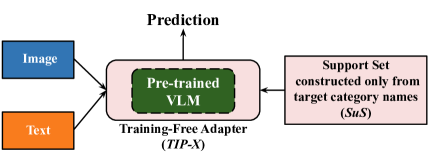
Figure 1: Training-free name-only transfer. We propose SuS-X, a framework for enhancing the zero-shot transfer abilities of VLMs like CLIP [61], BLIP [46] and TCL [76], without training. To achieve this, we propose a novel method TIP-X, which adapts these VLMs using a curated support set (SuS) that is not drawn from the target distribution. Our SuS leverages one key piece of information about the task at hand: the names of the target categories.

Table 1: Taxonomy of CLIP adaptation methods for downstream classification. We underline the Zero-Shot CLIP model to signify that it is the base model that all others build on top of. ^∗This method considers access to all test-set samples simultaneously, hence we still consider it zero-shot. ^†This method additionally uses class hierarchy maps.

	Method	Does not require	Does not require	Does not require
		training	labelled data	target data distribution
Few-shot fine-tuning methods	LP-CLIP [61]	✗	✗	✗
	CoOp [88]	✗	✗	✗
	PLOT [12]	✗	✗	✗
	LASP [10]	✗	✗	✗
	SoftCPT [21]	✗	✗	✗
	VT-CLIP [83]	✗	✗	✗
	VPT [19]	✗	✗	✗
	ProDA [49]	✗	✗	✗
	CoCoOp [87]	✗	✗	✗
	CLIP-Adapter [28]	✗	✗	✗
Intermediate methods	TIP-Adapter [84]	✓	✗	✗
	UPL [40]	✗	✓	✗
	SVL-Adapter [58]	✗	✓	✗
	TPT [52]	✗	✓	✓
	CLIP+SYN [36]	✗	✓	✓
	CaFo [82]	✗	✓	✓
Zero-shot methods	Zero-Shot CLIP [61]	✓	✓	✓
	CALIP [34]	✓	✓	✓
	CLIP+DN [89]∗	✓	✓	✓
Training-free name-only transfer methods	CuPL [60]	✓	✓	✓
	VisDesc [53]	✓	✓	✓
	CHiLS [57]†	✓	✓	✓
	SuS-X (ours)	✓	✓	✓

One such prominent model, CLIP [61], is trained on a web-scale corpus of 400M image-text pairs using a contrastive loss that maximises the similarities of paired image-text samples. CLIP pioneered the notion of zero-shot transfer in the vision-language setting: classification on unseen datasets. For a given classification task, CLIP converts the class labels into classwise textual prompts. An example of such a prompt is “A photo of a $<$CLASS$>$.”, where $<$CLASS$>$ is replaced by the ground-truth text label for each class. It then computes similarities between the query image and text prompts of all classes. The class whose prompt yields the maximal similarity with the query image is then chosen as the predicted label.

The zero-shot performance of CLIP is however limited by its pre-training distribution [27, 64, 24, 55]. If the downstream dataset distribution diverges too strongly from the distribution of images seen during pretraining, CLIP’s zero-shot performance drastically drops [24]. To mitigate this, several lines of work propose to adapt CLIP on diverse downstream tasks—Tab. 1 provides a brief summary of these methods. Most of them employ fine-tuning on either labelled or unlabelled subsets of data from the target task. However, fine-tuning such an over-parameterised model can be unstable and lead to overfitting [17, 28]. Furthermore, having access to the true distribution of the target task can be prohibitive in data-scarce environments [13, 4, 42] and online learning settings [16, 69].

To alleviate these issues, in this paper, we aim to adapt CLIP and other VLMs for downstream classification in a name-only (requires only category names, but no samples from the target task) and training-free fashion. We propose SuS-X (see Fig. 1), consisting of two novel building blocks: (i) SuS (Support Sets), our dynamic support set curation strategy that forgoes the need for samples from the target task, and (ii) TIP-X, our main framework for performing zero-shot classification while being training-free. For a given downstream task, we first curate a support set by leveraging the task category labels, either in a parametric manner i.e., generating images from large-scale text-to-image models (e.g., Stable Diffusion [63]) or non-parametric manner i.e., retrieving real-world images from a large vision-language data bank (e.g., LAION-5B [65]). We then use the curated support set as a proxy few-shot dataset to inform our downstream predictions using TIP-X, in a similar vein to recent few-shot adaptation methods [28, 84].

Our extensive experiments show that SuS-X outperforms zero-shot methods on 19 benchmark datasets across three VLMs, namely, CLIP, BLIP and TCL by 4.60%, 5.97% and 11.37% absolute average accuracy respectively. We further extend the TIP-X framework to the few-shot regime, outperforming previous SoTA methods in the training-free domain. Our main contributions are three-fold: (1) We propose SuS-X, a SoTA method in the training-free name-only transfer setting for downstream adaptation of VLMs, (2) We present SuS, an effective strategy for curating support sets using parametric or non-parametric methods to mitigate the lack of data samples available from the target task distribution, and (3) We propose TIP-X, a novel training-free method for adapting VLMs to downstream classification in both the name-only transfer and few-shot regimes.

2 Related Work

Vision-Language (VL) Foundation Models. In the past few years, there has been a Cambrian explosion in large-scale VL foundation models [6]. In a seminal work, Radford et al. [61] introduced CLIP, a large VLM trained on a massive corpus (400M image-text pairs acquired from the web) that exhibits strong downstream visual task performance. The introduction of CLIP inspired further development of VLMs [46, 1, 41, 20, 85, 79, 76, 11, 74, 29, 31, 47, 50, 78], each pre-trained on web-scale datasets to learn joint image-text representations. These representations can then be applied to tackle downstream tasks like semantic segmentation [67, 30], object detection [33, 23], image captioning [54, 3] and generative modelling [63, 62], In this work, we adapt such VLMs in a training-free setting to diverse downstream tasks.
Adaptation of VL models. The paradigm shift introduced by CLIP is its ability to do image classification in a zero-shot transfer setting [61]. In this setup, none of the target dataset classes are known a-priori and the task is to adapt implicitly at inference time to a given dataset. Since CLIP’s training objective drives it to assign appropriate similarities to image-text pairs, it acquires the ability to perform zero-shot classification directly.

Inspired by CLIP’s zero-shot success, further work has sought to improve upon its performance. In Tab. 1, we characterise some of these methods along three major axes: (i) if the method requires training, (ii) if the method requires labelled samples from the target task, and (iii) if the method requires samples from the target task distribution.

In this work, we focus on the training-free name-only transfer regime—our goal is to adapt VLMs to target tasks without explicit training or access to samples from the target distribution. Instead, we assume access only to category names of target tasks. This formulation was recently considered for semantic segmentation, where it was called name-only transfer [66]—we likewise adopt this terminology. To the best of our knowledge, only two other concurrent approaches, CuPL [60] and VisDesc [53], operate in this regime. They use pre-trained language models to enhance textual prompts for zero-shot classification. By contrast, SuS-X pursues a support set curation strategy to adapt VLMs using knowledge of category names. These approaches are complementary, and we find that they can be productively combined. Two other related works operating purely in the zero-shot setting are: (1) CALIP [34], which uses parameter-free attention on image-text features, and (2) CLIP+DN [89], which uses distribution normalisation. We compare with these four baselines in Sec. 4.

3 SuS-X: Training-Free Name-Only Transfer

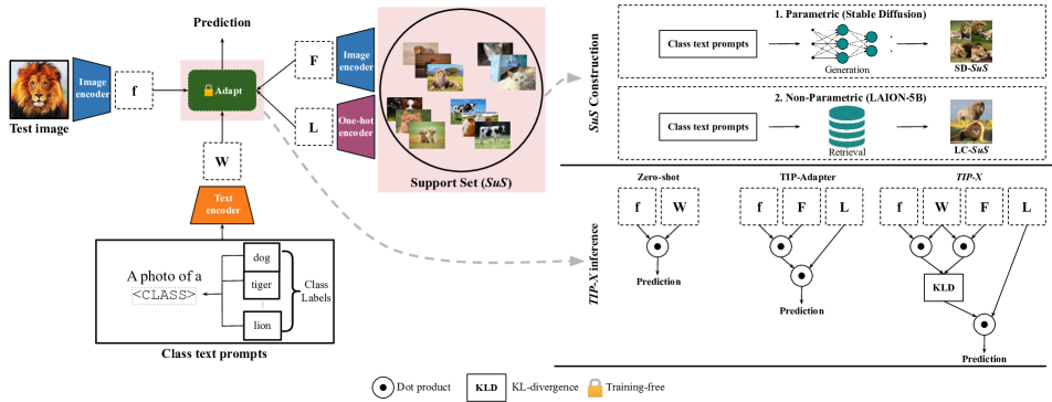
Figure 2: SuS-X for training-free name-only transfer. SuS-X consists of two core building blocks. (1) SuS (top right), a dynamic support set that we construct to infuse visual information into the VLM based only on knowledge of target category names. We construct support sets either in a parametric (generating images using Stable Diffusion) or non-parametric (retrieving images from LAION-5B) manner. (2) TIP-X (bottom right), our novel training-free method that leverages image-text distances to compute similarities between the support set and the test images. These similarities act as attention weights for the support set labels, and can directly be combined with the original logits from the VLM for classification.

We describe the two main building blocks of SuS-X—(1) Support Set (SuS) construction, and (2) training-free inference using our novel TIP-X method. Fig. 2 depicts our overall training-free name-only transfer framework.

3.1 SuS Construction

We follow recent adaptation methods [84, 28] that use a small collection of labelled images to provide visual information to CLIP. However, differently from these methods, rather than accessing labelled images from the target distribution, we propose two methods (described next) to construct such a support set (SuS) without such access.

(I) Stable Diffusion Generation. Our first method leverages the powerful text-to-image generation model, Stable Diffusion [63]. We employ specific prompting strategies for generating salient and informative support images. Concretely, given a set of downstream textual class labels, $\mathcal{T}=\{t_{1},t_{2},\dots,t_{C}\}$, where $C$ denotes the number of categories, we prompt Stable Diffusion to generate $N$ images per class. In this way, we construct our support set of size $NC$, with each image having its associated class label.

By default, we prompt Stable Diffusion using the original CLIP prompts, i.e., “A photo of a $<$CLASS$>$.”, where $<$CLASS$>$ is the class text label. To further diversify the generation process, we follow CuPL [60] to first generate customised textual prompts for each class by prompting GPT-3 [8] to output descriptions of the particular class. We then feed this customised set of prompts output by GPT-3 into Stable Diffusion for generating images. For example, to generate images from the “dog” class, we prompt GPT-3 to describe “dogs”, and then prompt Stable Diffusion with the resulting descriptions. In section 4.4, we compare the performance of the default (called Photo) and this augmented prompting procedure (called CuPL). Unless otherwise specified, all our experiments with Stable Diffusion support sets use the CuPL strategy.

(II) LAION-5B Retrieval. Our second method leverages the large-scale vision-language dataset, LAION-5B [65]. It contains 5.85 billion image-text pairs, pre-filtered by CLIP. Using LAION-5B, we retrieve task-specific images using class text prompts for constructing the support set. Concretely, given textual class labels, $\mathcal{T}=\{t_{1},t_{2},\dots,t_{C}\}$, we rank all images in LAION-5B by their CLIP image-text similarity to each text class label $t_{i}$, where $i\in[1,C]$. We then use the top $N$ image matches as our support set for class $i$, resulting in an $NC$-sized support set of images with their associated class labels. Note that curating supporting knowledge by search is a classical technique in computer vision [26] that was recently revisited in the task of semantic segmentation [67]. Here we adapt this idea to the name-only transfer classification setting. For efficient retrieval, we leverage the approximate nearest neighbour indices released by the authors. Similar to the Stable Diffusion generation approach, we experiment with both Photo and CuPL prompting strategies for curating our LAION-5B support set (see Sec. 4.4). By default, we use Photo prompting for all our experiments with LAION-5B support sets.

Remark. Note that SuS can be seen as a visual analogue to CuPL [60], where, for each class, we augment VLMs with rich, relevant images, instead of the customised textual descriptions generated in CuPL.

3.2 TIP-X Inference

Given our support set from the previous section, our task is to now leverage it in a training-free inference scheme to inform CLIP’s zero-shot predictions. We first briefly review the zero-shot CLIP classification pipeline, discuss the recently proposed TIP-Adapter [84] for training-free adaptation, and highlight a critical shortcoming in its method due to uncalibrated intra-modal embedding distances, which we address in our method—TIP-X.

Zero-shot CLIP. For classification into $C$ classes, CLIP converts class labels into text prompts and encodes them with its text encoder. Collectively, the encoded prompt vectors can be interpreted as a classifier weight matrix $W\in\mathbb{R}^{C{\times}d}$, where $d$ is embedding dimension. For a test set ${T}{=}{\{y_{1},y_{2},...,y_{t}\}}$ comprising $t$ test images, CLIP’s image encoder is applied to produce test image features:

$$\begin{gathered}f_{i}=\texttt{CLIPImageEncoder}(y_{i}),i\in[1,t],f_{i}\in\mathbb{R}^{d}\\ f=\texttt{Concat}([f_{1},f_{2},\dots,f_{t}]),f\in\mathbb{R}^{t\times d}\end{gathered}$$ (1)

Using $W$ and $f$, CLIP performs classification by computing zero-shot logits (ZSL) via a dot product:

$$\texttt{ZSL}=fW^{T}$$ (2)

TIP-Adapter. Given a $CK$-sized $K$-shot labelled dataset $D=\{x_{1},x_{2},\dots,x_{CK}\}$ from the target domain, TIP-Adapter [84] encodes $D$ using CLIP’s image encoder:

$$\begin{gathered}F_{i}=\texttt{CLIPImageEncoder}(x_{i}),i\in[1,CK],F_{i}\in\mathbb{R}^{d}\\ F=\texttt{Concat}([F_{1},F_{2},\dots,F_{CK}]),F\in\mathbb{R}^{CK\times d}\end{gathered}$$ (3)

It then converts each of the few-shot class labels to one-hot vectors $L\in\mathbb{R}^{CK{\times}C}$. Next, it computes an affinity matrix to capture the similarities between $F$ and $f$:

$$A=\exp(-\beta(1-fF^{T}))$$ (4)

where $\beta$ is a hyperparameter that modulates “sharpness”. Finally, these affinities are used as attention weights over $L$ to produce logits that are blended with ZSL using a hyperparameter, $\alpha$:

$$\texttt{TL}=\alpha AL+fW^{T}$$ (5)

Motivating TIP-X. TIP-Adapter gains from the affinity computation between the test and few-shot image samples (see Eq. 4). This similarity is computed in CLIP’s image space. However, prior research [80, 48, 70] has demonstrated the existence of a modality gap between CLIP’s image and text spaces. This leads us to question if doing image-image similarity comparisons in CLIP’s image space is optimal.

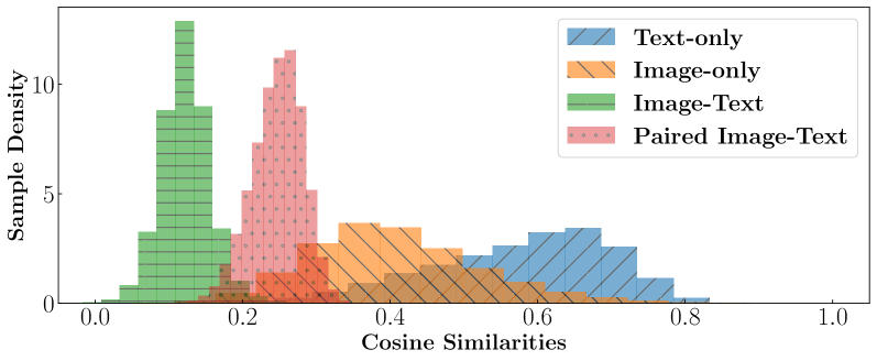
(a) Intra-modal and inter-modal CLIP cosine similarities. We observe quite distinct intra-modal and inter-modal cosine similarity distributions.

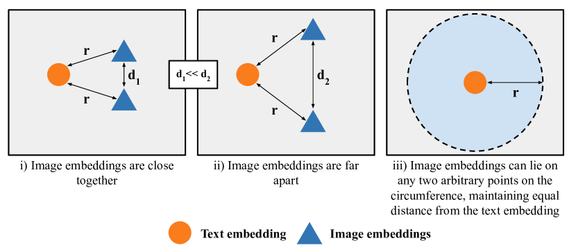
(b) Intra-modal degrees of freedom. Different intra-modal similarities can satisfy same inter-modal constraints, leaving room for poor calibration.

Figure 3: Our two-fold analysis motivating TIP-X

Fig. 3(a) shows the pairwise image-image, text-text and image-text cosine similarities of the ImageNet validation set CLIP embeddings. Clearly, the intra-modal and inter-modal similarities are distributed differently—the inter-modal similarities have small variance and mean, whereas the intra-modal similarities have larger means and variances. This mismatch happens because contrastive training of CLIP maximises the inter-modal cosine similarities of paired samples without regard to intra-modal similarities. This implies that the intra-image CLIP embedding similarities employed by TIP-Adapter may not reflect the true intra-image similarities. Fig. 3(b) illustrates this idea with a simple example. Consider two image embeddings that are required to be a distance $r$ away from a particular text embedding. The two image embeddings can satisfy this condition by being very close to each other or very far apart from each other. Fig. 3(b) shows that this constraint can be satisfied by any two arbitrary points on a hypersphere of radius $r$. While we expect loose constraints to be imposed via transitivity, we nevertheless expect a lower quality of calibration in intra-modal (e.g., image-image) comparisons.

TIP-X to the rescue. To get around the problem of uncalibrated intra-modal embedding distances in TIP-Adapter, we propose to use inter-modal distances as a bridge. More specifically, rather than computing similarities between the test features ($f{\in}\mathbb{R}^{t{\times}d}$) and few-shot features ($F{\in}\mathbb{R}^{CK\times d}$) in the image embedding space ($fF^{T}$), we use the image-text space. We first construct signatures by computing similarities of $f$ and $F$ with the text classifier weights $W$:

$$\begin{gathered}S=\texttt{softmax}(FW^{T}),S\in\mathbb{R}^{CK\times C}\\ s=\texttt{softmax}(fW^{T}),s\in\mathbb{R}^{t\times C}\end{gathered}$$ (6)

These signatures comprise probability distributions encoding inter-modal affinities between the few-shot features and class text vectors, and likewise for the test features. We then construct our affinity matrix $M\in\mathbb{R}^{t\times CK}$ by measuring the KL-divergence between the signatures as follows:

$$\begin{gathered}M_{i,j}=\texttt{KL}(s_{i}||S_{j}),i\in[1,t],j\in[1,CK]\end{gathered}$$ (7)

where $s_{i}$ represents the $i^{th}$ test signature for the $t$ test samples, and $S_{j}$ represents the $j^{th}$ few-shot signature. Since we are working with discrete probability distributions, we compute the KL-divergence as $\texttt{KL}(P||Q)=\sum_{i}P_{i}\log\frac{P_{i}}{Q_{i}}$.

The construction of the affinity matrix $M$ can be seen as analogous to the affinity computation in TIP-Adapter (Eq. 4). However, our affinity matrix construction removes direct reliance on the uncalibrated image-image similarities.

Finally, before using our affinity matrix $M$ as attention weights for $L$ (one-hot encoded class labels), we rescale (denoted by $\psi$) the values of $M$ to have the same range (min, max values) as the TIP-Adapter affinities ($A$). Further, since our affinity matrix $M$ consists of KL-divergence values, the most similar samples will get small weights since their KL-divergence will be low (close to 0). To mitigate this, we simply negate the values in $M$. We then blend our predicted logits with TL using a scalar $\gamma$:

$$\texttt{TXL}=fW^{T}+\alpha AL+\gamma\psi(-M)L$$ (8)

The entire TIP-X method is shown in  Fig. 2 (bottom right).

3.3 SuS-X: Combining SuS and TIP-X

Since our constructed support sets act as pseudo few-shot datasets, we directly replace the few-shot features $F$ in the TIP-X framework with the features of our support set. We call our method SuS-X-LC if we combine TIP-X with the LAION-5B curated support set, and SuS-X-SD when combined with the Stable Diffusion generated support set. These methods enable training-free name-only adaptation of zero-shot VLMs.

4 Experiments

First, we evaluate SuS-X against strong baselines in the training-free zero-shot/name-only transfer regimes, across three VLMs. Next, we illustrate the adaptation of TIP-X into the few-shot training-free regime. Finally, we ablate and analyse our method to provide additional insights.

4.1 Training-free name-only transfer evaluation

Datasets. For a comprehensive evaluation, we test on 19 datasets spanning a wide range of object, scene and fine-grained categories: ImageNet [18], StanfordCars [43], UCF101 [68], Caltech101 [25], Caltech256 [32], Flowers102 [56], OxfordPets [59], Food101 [7], SUN397 [75], DTD [14], EuroSAT [37], FGVCAircraft [51], Country211 [61], CIFAR-10 [44], CIFAR-100 [44], Birdsnap [5], CUB [72], ImageNet-Sketch [73] and ImageNet-R [38]. Previous few-shot adaptation methods [81, 28, 86] benchmark on a subset of 11 of these 19 datasets. We report results on the 19-dataset suite in the main paper and compare results using only the 11-dataset subset in the supp. mat.

Experimental Settings. We compare against six baselines. For zero-shot CLIP, we use prompt ensembling with 7 different prompt templates following [61, 84]. We run CuPL, VisDesc (name-only transfer) and CLIP+DN (zero-shot transfer) using their official code. We also experiment with augmenting the CuPL prompts with the original prompt ensemble, and call it CuPL+e. For CALIP (zero-shot transfer), in the absence of public code at the time of writing, we aim to reproduce their results using our own implementation. For our proposed methods, we report results using both SuS-X-LC and SuS-X-SD. For both methods, we use a fixed number of support samples per dataset (see supp. mat. for details). For CALIP and SuS-X, we conduct a hyperparameter search on the dataset validation sets. In Sec. 4.4 we perform a hyperparameter sensitivity test for a fair evaluation. By default, we use the ResNet-50 [35] backbone as CLIP’s image encoder for all models.

Table 2: Training-free adaptation of CLIP on 19 datasets with RN50 visual backbone. The best and second best results for each dataset are bolded and underlined, respectively. Individual results for all 19 datasets are available in the supp. mat. ^∗Average reported across 19 datasets. ^†Our re-implementation.

	Method	Average∗	ImageNet [18]	ImageNet-R [38]	ImageNet-Sketch [73]	EuroSAT [37]	DTD [14]	Birdsnap [5]
Zero-shot	Zero-shot CLIP [61]	52.27	60.31	59.34	35.42	26.83	41.01	30.56
	CALIP [34]	–	60.57	–	–	38.90	42.39	–
	CALIP [34]†	52.37	60.31	59.33	36.10	26.96	41.02	30.68
	CLIP+DN [89]	53.02	60.16	60.37	35.95	28.31	41.21	31.23
Name-only	CuPL [60]	55.50	61.45	61.02	35.13	38.38	48.64	35.65
	CuPL+e	55.76	61.64	61.17	35.85	37.06	47.46	35.80
	VisDesc [53]	53.76	59.68	57.16	33.78	37.60	41.96	35.65
	SuS-X-SD (ours)	56.73	61.84	61.76	36.30	45.57	50.59	37.14
	SuS-X-LC (ours)	56.87	61.89	62.10	37.83	44.23	49.23	38.50

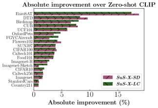
(a)

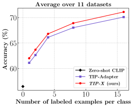
(b)

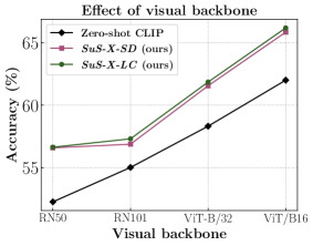
(c)

Figure 4: (a) Comparison of SuS-X with Zero-shot CLIP. (b) Results of training-free few-shot classification. (c) Performance comparison of SuS-X across visual backbones.

Main Results. In Tab. 2, we compare both variants of SuS-X with the baselines. We report an average across 19 datasets. We also include results on ImageNet, EuroSAT, DTD, Birdsnap, ImageNet-R and ImageNet-Sketch (results on all 19 datasets in the supp. mat.). SuS-X methods outperform zero-shot CLIP by 4.6% on average across all 19 datasets. We observe striking gains of 18%, 8% and 7% on EuroSAT, DTD and Birdsnap respectively. We also outperform the SoTA training-free adaptation methods—CuPL+ensemble and VisDesc by 1.1% and 3.1% on average respectively. To further probe where we attain the most gains, we plot the absolute improvement of our models over zero-shot CLIP in Fig. 4(a). We observe large gains on fine-grained (Birdsnap, CUB, UCF101) and specialised (EuroSAT, DTD) datasets, demonstrating the utility of SuS-X in injecting rich visual knowledge into zero-shot CLIP (additional fine-grained classification analysis in supp. mat.). We further compare SuS-X to few-shot methods that use labelled samples from the true distribution in the supp. mat.—despite being at a disadvantage due to using no target distribution samples, SuS-X is still competitive with these methods.

4.2 Transfer to different VLMs

We evaluate transfer to VLMs other than CLIP, namely TCL [76] and BLIP [46]. We only retain image and text encoders of these models for computing features, while preserving all other experimental settings from Sec. 4.1. Tab. 3 shows our SuS-X methods strongly outperform all baseline methods across both VLMs—we improve on zero-shot models by 11.37% and 5.97% on average across 19 datasets. This demonstrates that our method is not specific to CLIP, but can improve performance across different VLMs.

Table 3: SuS-X generalises to different VLMs. ^∗Average reported across 19 datasets.

VLM	Method	Average∗	ImageNet	EuroSAT	DTD	Birdsnap
TCL	Zero-shot	31.38	35.55	20.80	28.55	4.51
	CuPL	34.79	41.60	26.30	42.84	6.83
	CuPL+e	32.79	41.36	25.88	41.96	6.60
	VisDesc	33.94	40.40	21.27	34.28	5.69
	SuS-X-SD	41.49	52.29	28.75	48.17	13.60
	SuS-X-LC	42.75	52.77	36.90	46.63	17.93
BLIP	Zero-shot	48.73	50.59	44.10	44.68	10.21
	CuPL	51.11	52.96	39.37	52.95	12.24
	CuPL+e	51.36	53.07	41.48	53.30	12.18
	VisDesc	49.91	50.94	42.25	47.45	11.69
	SuS-X-SD	53.20	55.93	45.36	56.15	16.95
	SuS-X-LC	54.64	56.75	51.62	55.91	23.78

4.3 Adapting to the few-shot regime

A key component of our SuS-X method is TIP-X. In the previous section, we showcased SoTA results in the training-free name-only transfer regime. Due to its formulation, TIP-X can directly be extended to the few-shot regime, where our support sets are labelled samples from the target dataset rather than curated/generated samples. To evaluate TIP-X on such real-world support sets, we conduct training-free few-shot classification using TIP-X. We compare against the SoTA method in this regime—TIP-Adapter [84]. We report results on the 11-dataset subset used by TIP-Adapter on five different shot settings of the $K$-shot classification task: 1, 2, 4, 8 and 16.

We present average accuracy results on all shots in Fig. 4(b)—TIP-X outperforms both Zero-shot CLIP and TIP-Adapter (absolute gain of 0.91% across shots). Notably, on OxfordPets, we achieve 2.1% average gain. This further demonstrates the generalisability of the TIP-X method in transferring to the few-shot training-free setting.

4.4 Analysis

We conduct several ablations and provide additional visualisations to offer further insight into the SuS-X method.

Component Analysis. SuS-X consists of two major building blocks—SuS construction and TIP-X. We compare the performance difference (with average accuracy across 19 datasets) of using SuS with TIP-Adapter instead of TIP-X in Tab. 4. We use both default ensemble prompts and CuPL prompts for CLIP’s text classifier to break down the performance gains further. We note that both SuS and TIP-X are crucial for achieving the best results.

(a)

(b)

(c)

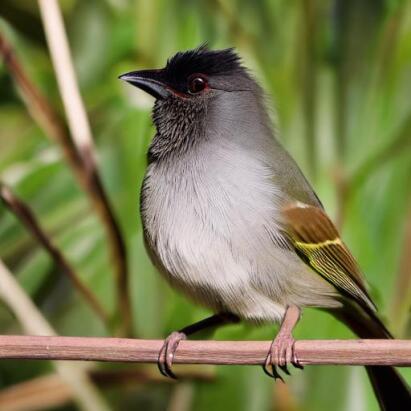
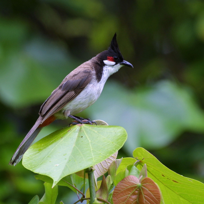
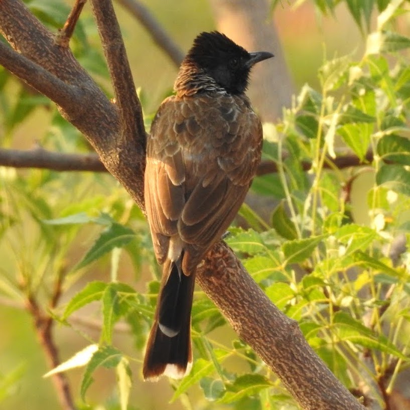
(d)

Figure 5: Support samples from the generated SuS-SD, retrieved SuS-LC and true training distribution for ImageNet. By randomising the image order in each subfigure, we pose a challenge question—can you match the three images for each subfigure to their source i.e. SuS-SD, SuS-LC or ImageNet train set? The answers are provided at the bottom of the page.

Transfer to different visual backbones. We evaluate the scalability of our model across different CLIP visual backbones— Fig. 4(c) shows that both SuS-X variants consistently improve upon zero-shot CLIP across ResNet and VisionTransformer backbones of varying depths and sizes.

SuS size. We study the effect of varying support set size for SuS-LC and SuS-SD—we generate three different support sets with random seeds for support sizes of 1, 5, 10, 25, 50, 75 and 100 samples. From Fig. 6, we observe two broad trends—some tasks benefit (ImageNet-R, DTD) from having more support set samples while others do not (Country211, Flowers102). We suggest that this is connected to the domain gap between the true data distribution and support set samples—if the domain gap is large, it is inimical to provide a large support set, whereas if the domains are similar, providing more support samples always helps.

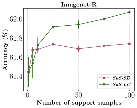
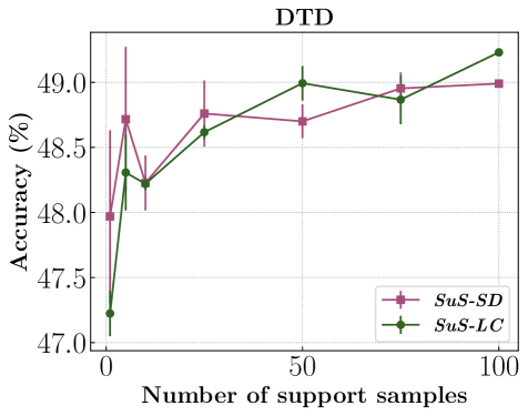
(a)

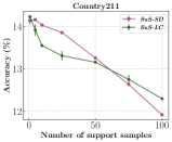
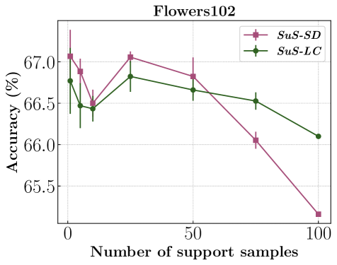
(b)

Figure 6: Effect of support size.

SuS visualisation. We visualise samples from both support set construction methods on ImageNet in Fig. 5. It is hard to distinguish between the true ImageNet samples and the SuS samples—we can therefore construct support sets to mimic the true data distribution, with access to only the category names. A caveat is that the support set does not always capture the domain characteristics of the true distribution, leading to a domain gap (lighting conditions, diverse scene backgrounds, confounding objects etc). To fully close the gap to using true few-shot datasets as support sets [28, 84], further research into exact unsupervised domain matching of support sets and few-shot datasets is required.

Prompting strategies for SuS construction. Tab. 5 depicts the performance of Photo and CuPL prompting—best results are achieved with the LC-Photo and SD-CuPL strategies. We further compare the diversity of images produced by the two strategies on ImageNet—from Tab. 5, it is evident that CuPL prompting leads to more diverse support sets as compared to Photo prompting.

Table 4: Component Analysis of SuS-X.

Text Prompts	Method	SuS	TIP-X	Average Accuracy
Default	Zero-shot CLIP	✗	✗	52.27
	SuS-TIP-SD	✓	✗	53.49 (+1.22%)
	SuS-X-SD	✓	✓	53.69 (+1.42%)
	SuS-TIP-LC	✓	✗	53.83 (+1.56%)
	SuS-X-LC	✓	✓	54.20 (+1.93%)
CuPL+e	CuPL+e	✗	✗	55.76 (+3.49%)
	SuS-TIP-SD	✓	✗	56.63 (+4.36%)
	SuS-X-SD	✓	✓	56.73 (+4.46%)
	SuS-TIP-LC	✓	✗	56.72 (+4.45%)
	SuS-X-LC	✓	✓	56.87 (+4.60%)

Table 5: Prompting strategies for SuS construction.

SuS method	Average Acc.		ImageNet Acc.		Diversity
	Photo	CuPL	Photo	CuPL	Photo	CuPL
LC	56.87	56.20	61.89	61.79	0.28	0.32
SD	56.32	56.73	61.79	61.84	0.17	0.20

Hyperparameter Sensitivity. We perform a sensitivity test for our $\gamma$ hyperparameter (refer Eq. 8) on ImageNet-R, OxfordPets, and DTD. We fix $\alpha$ and $\beta$ to be 1, and run a sweep over $\gamma\in[0,1]$. From Tab. 6, we observe that moderate values of $\gamma$ are typically preferred, and the variance of the accuracy values is small. However, note that for DTD, the optimal $\gamma$ is slightly larger (0.75)—this is due to its specialised nature which requires more guidance from the specialised support set to inform pre-trained CLIP. Previous few-shot adaptation works [28, 84] observed similar results. For more hyperparameter ablations, see the supp. mat.

Table 6: Hyperparameter sensitivity for $\boldsymbol{\gamma}$

Dataset	$\boldsymbol{\gamma}$ value
	$\boldsymbol{0}$	$\boldsymbol{0.1}$	$\boldsymbol{0.2}$	$\boldsymbol{0.3}$	$\boldsymbol{0.5}$	$\boldsymbol{0.75}$	$\boldsymbol{1}$
ImageNet-R	60.87	60.98	61.03	61.05	61.00	60.89	60.65
OxfordPets	76.76	77.17	77.58	77.44	77.17	77.17	76.90
DTD	47.16	47.16	47.51	47.69	47.87	47.96	47.60

4.5 Limitations and broader impact

While demonstrating promising results, we note several limitations of our approach. (1) To perform name-only transfer, we rely on CLIP to have seen related concepts during pre-training. For concepts that are so rare that they do not appear during pre-training, transfer will not be feasible. (2) We employ LAION-5B [65] as a source of knowledge. While reasonable for a proof of concept, this data is relatively uncurated and may contain harmful content. As such, our approach is not suitable for real-world deployment without careful mitigation strategies to address this concern. Similar arguments apply to Stable Diffusion [63].

5 Conclusion

In this paper, we studied the training-free name-only transfer paradigm for classification tasks. We systematically curated support sets with no access to samples from the target distribution and showed that they help improve CLIP’s zero-shot predictions by providing rich, task-specific knowledge. We further motivated the TIP-X framework through the observation that CLIP’s intra-modal embedding spaces are not optimal for computing similarities. With these two building blocks, we demonstrated superior performance to prior state-of-the-art.

Acknowledgements. This work was supported by the Isaac Newton Trust and an EPSRC access-to-HPC grant. SA would like to acknowledge the support of Z. Novak and N. Novak in enabling his contribution. VU would like to thank Gyungin Shin, Surabhi S. Nath, Jonathan Roberts, Vlad Bogolin, Kaiqu Liang and Anchit Jain for helpful discussions and feedback.

Appendix A Dataset Details

We enumerate the validation and testing split sizes of all datasets in Tab. 7. We make two small modifications to the standard datasets as described in CoOp [86]: (1) We discard the “BACKGROUND Google” and “Faces easy classes” from the Caltech101 dataset, and (2) For the UCF101 dataset, we consider the middle frame of each video as our image sample.

Table 7: Dataset details for the 19 datasets used in this study.

Dataset	Classes	Val	Test
UCF-101	101	1898	3783
CIFAR-10	10	10000	10000
CIFAR-100	100	10000	10000
Caltech101	100	1649	2465
Caltech256	257	6027	9076
ImageNet	1000	50000	50000
SUN397	397	3970	19850
FGVCAircraft	100	3333	3333
Birdsnap	500	7774	11747
StanfordCars	196	1635	8041
CUB	200	1194	5794
Flowers102	102	1633	2463
Food101	101	20200	30300
OxfordPets	37	736	3669
DTD	47	1128	1692
EuroSAT	10	5400	8100
ImageNet-Sketch	1000	50889	50889
ImageNet-R	200	30000	30000
Country211	211	10550	21100

Appendix B Details about Support Set Curation Strategies

We include further technical details about our two support set curation strategies—Stable Diffusion Generation and LAION-5B Retrieval.

Stable Diffusion Generation. For all our experiments with the Stable Diffusion model, we use the stable-diffusion-v1-4 checkpoint with a 9.5 guidance scale [39], 85 diffusion steps and $512{\times}512$ output resolution. We then downscale these images to CLIP’s input resolution of $224{\times}224$.

LAION-5B Retrieval. For all our experiments, we rank all images in the LAION-5B corpus based on their image-text similarity with the given class textual prompt. We use the LAION-5B pre-constructed index that leverages the CLIP-ViT-L/14 model. Finally, since the images might be of varying resolutions, we pre-process them to CLIP’s input resolution of $224{\times}224$.

Appendix C Few-shot Learning with TIP-X

In Sec. 4.3, we adapt TIP-X to the few-shot training-free adaptation regime, and compare with the SoTA model TIP-Adapter. We now show the extended results on all 11 datasets in Fig. 7. On average, we outperform TIP-Adapter by $0.91\%$ across all shots.

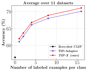
(a)

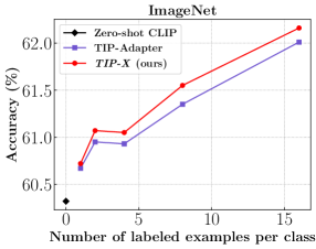
(b)

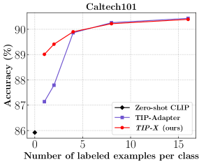
(c)

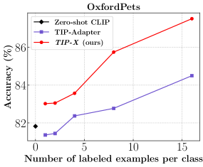
(d)

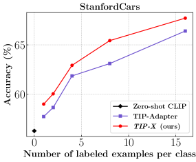
(e)

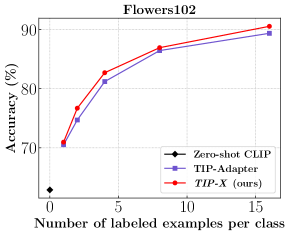
(f)

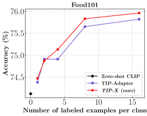
(g)

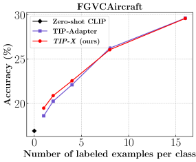
(h)

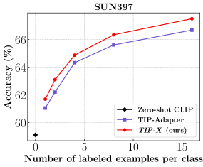
(i)

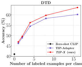
(j)

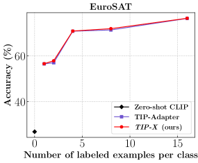
(k)

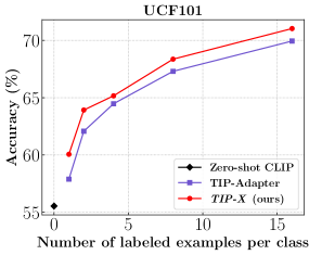
(l)

Figure 7: Results for the training-free few-shot regime across 11 datasets.

Appendix D Details about Support Set Sizes

For our main results in Sec. 4.1, we use a fixed number of support set samples per dataset. In Tab. 8, we enumerate the number of support set samples used per dataset. As shown in Sec. 4.4, the support set size can impact performance significantly—the nature of these impacts are dataset-specific.

Table 8: Support Set Sizes

Dataset	Support Set Size
UCF-101	5858
CIFAR-10	50
CIFAR-100	4700
Caltech101	101
Caltech256	3084
ImageNet	36000
SUN397	397
FGVCAircraft	7900
Birdsnap	39000
StanfordCars	980
CUB	400
Flowers102	3162
Food101	3434
OxfordPets	2627
DTD	188
EuroSAT	150
ImageNet-Sketch	42000
ImageNet-R	10200
Country211	844

Appendix E Details about Baselines

For our main zero-shot/name-only training-free CLIP-based experiments, we use six main baselines—Zero-shot CLIP [61], CALIP [34], CLIP+DN [89], VisDesc [53], CuPL [60] and CuPL+e.

Zero-shot CLIP. For Zero-shot CLIP, we directly use the model weights released by OpenAI and the official repository for reproducing results on different datasets. For benchmarking all our results, we use the 7-prompt ensemble set used by TIP-Adapter [84] for all datasets. The 7 prompt templates in the ensemble are: “itap of a $<$class$>$.”, “a origami $<$class$>$.”, “a bad photo of the $<$class$>$.”, “a photo of the large $<$class$>$.”, “a $<$class$>$ in a video game.”, “art of the $<$class$>$.”, and “a photo of the small $<$class$>$.”.

CALIP details. Due to the unavailability of publicly released code at the time of writing this paper, we re-implement the CALIP baseline, following the description in [34]. We provide access to our re-implementation as part of our released codebase.

CLIP+DN details. For CLIP+DN, we use the official code released by the authors on all datasets. As specified in the paper, we (i) use 100 random unlabeled validation samples for the mean estimation for DN, and (ii) report the average accuracy across 5 different random seeds.

VisDesc details. For VisDesc, we use the official code released by the authors on all datasets. We use their default prompt settings for generating the GPT-3 descriptors.

CuPL details. For CuPL, we use the official code released by the authors on all datasets. The list of pre-prompts used as inputs to GPT-3 for different datasets are listed in Tab. 9 and Tab. 10.

CuPL+e details. For CuPL+e, we simply concatenate the 7-prompt ensemble embeddings of each class with the custom GPT-3 generated CuPL embeddings of that particular class. We then average all the embeddings within a class to generate the textual embedding for that class. Then, we proceed as standard to construct the classifier weight matrix by stacking all class text embeddings.

E.1 Transfer to other VLMs

We can transfer all the aforementioned baselines to different VLMs by simply swapping out CLIP’s frozen image and text encoders with those of TCL [76] and BLIP [46]. For the TCL experiments, we use the standard ViT-B/16 base model that is fine-tuned for retrieval on MS-COCO, released by the authors here. For the BLIP experiments, we use the standard ViT-B/16 base model fine-tuned for retrieval on MS-COCO, released by the authors here.

Table 9: CuPL hand-written prompts (1/2)

Dataset	GPT-3 prompts
UCF101	“What does a person doing {} look like”
	“Describe the process of {}”
	“How does a person {}”
CIFAR10	“Describe what a {} looks like”
	“How can you identify {}?”
	“What does {} look like?”
	“Describe an image from the internet of a {}”
	“A caption of an image of {}: ”
CIFAR100	“Describe what a {} looks like”
	“How can you identify {}?”
	“What does {} look like?”
	“Describe an image from the internet of a {}”
	“A caption of an image of {}: ”
Caltech101	“Describe what a {} looks like”
	“What does a {} look like”
	“Describe a photo of a {}”
Caltech256	“Describe what a {} looks like”
	“What does a {} look like”
	“Describe a photo of a {}”
ImageNet	“Describe what a {} looks like”
	“How can you identify {}?”
	“What does {} look like?”
	“Describe an image from the internet of a {}”
	“A caption of an image of {}: ”
SUN397	“Describe what a {} looks like”
	“How can you identify a {}?”
	“Describe a photo of a {}”
FGVCAircraft	“Describe a {} aircraft”
Birdsnap	“Describe what a {}, a species of bird, looks like”
	“What does a {} look like”
	“Visually describe a {}, a type of bird”
	“A caption of an image of a {}, a type of bird”
	“Describe the appearance of a {}”
	“What are the prominent features to identify a {} bird”
StanfordCars	“How can you identify a {}”
	“Description of a {}, a type of car”
	“A caption of a photo of a {}:”
	“What are the primary characteristics of a {}?”
	“Description of the exterior of a {}”
	“What are the identifying characteristics of a {}, a type of car?”
	“Describe an image from the internet of a {}”
	“What does a {} look like?”
	“Describe what a {}, a type of car, looks like”

Table 10: CuPL hand-written prompts (2/2)

Dataset	GPT-3 prompts
CUB	“Describe what a {}, a species of bird, looks like”
	“What does a {} look like”
	“Visually describe a {}, a type of bird”
	“A caption of an image of a {}, a type of bird”
	“Describe the appearance of a {}”
	“What are the prominent features to identify a {} bird”
Flowers102	“What does a {} flower look like”
	“Describe the appearance of a {}”
	“A caption of an image of {}”
	“Visually describe a {}, a type of flower”
Food101	“Describe what a {} looks like”
	“Visually describe a {}”
	“How can you tell that the food in this photo is a {}?”
OxfordPets	“Describe what a {} pet looks like”
	“Visually describe a {}, a type of pet”
DTD	“What does a {} material look like?”
	“What does a {} surface look like?”
	“What does a {} texture look like?”
	“What does a {} object look like?”
	“What does a {} thing look like?”
	“What does a {} pattern look like?”
EuroSAT	“Describe an aerial satellite view of {}”
	“How does a satellite photo of a {} look like”
	“Visually describe a centered satellite view of a {}”
ImageNet-Sketch	“Describe how a black and white sketch of a {} looks like”
	“A black and white sketch of a {}”
	“Describe a black and white sketch from the internet of a {}”
ImageNet-R	“An art drawing of a {}”
	“Artwork showing a {}”
	“A cartoon a {}”
	“An origami of a {}”
	“A deviant art photo depicting a {}”
	“An embroidery of a ”
	“A graffiti art showing a {}”
	“A painting of a {}”
	“A sculpture of a {}”
	“A black and white sketch of {}”
	“A toy of a {}”
	“A videogame of a {}”
Country211	“Visually describe what {} looks like”
	“What does the landscape of {} look like”
	“Describe a photo taken in {}”
	“How does a typical photo taken in {} look like”

Appendix F More SuS Visualisations

In Fig. 8, we provide further support set samples across different datasets curated using both SuS-LC and SuS-SD methods.

(a)

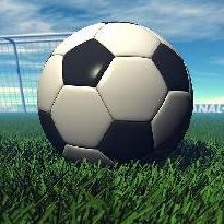
(b)

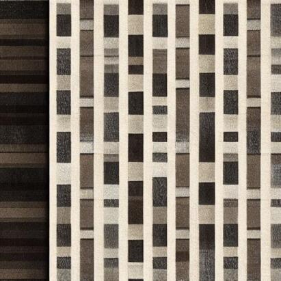
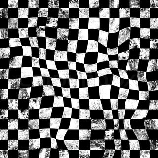
(c)

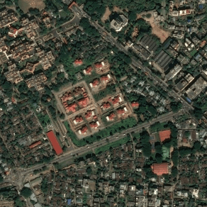
(d)

(e)

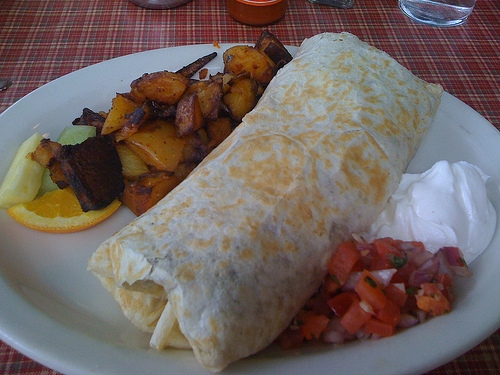
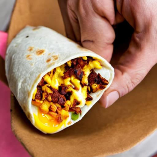
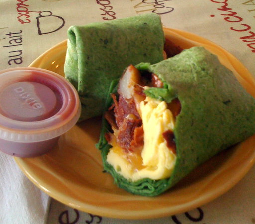
(f)

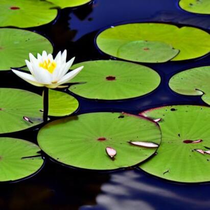
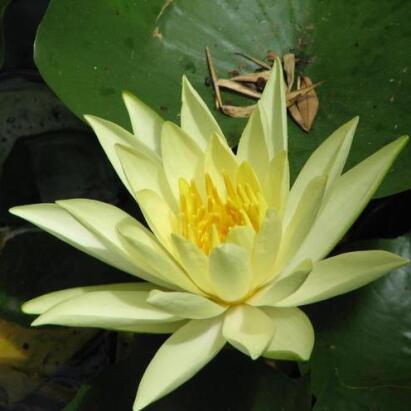
(g)

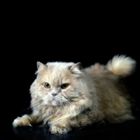
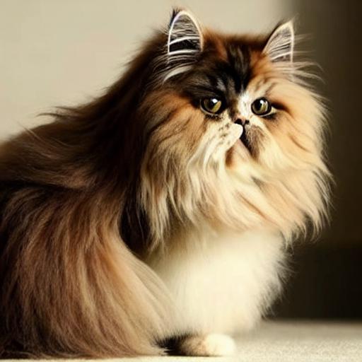
(h)

(i)

(j)

Figure 8: Support samples from the generated SuS-SD, retrieved SuS-LC and true training distribution for different datasets. For each subfigure, the ordering of figures is—SuS-LC, SuS-SD, Train. We label each figure with its source dataset and class name.

Appendix G Hyperparameter Settings

We provide the hyperparameter settings for obtaining our main results from Sec. 4.1 in Tab. 11. For our hyperparameters, we conduct a search over $[0.1,50]$ for $\alpha$, $[1,50]$ for $\beta$ and $[0.1,30]$ for $\gamma$. In the main paper, we have a hyperparameter sensitivity test which ensures that the variance in accuracy values is not too large as we vary our hyperparameters.

Table 11: Hyperparameter settings for the 19 datasets.

Dataset	$\boldsymbol{\alpha}$	$\boldsymbol{\beta}$	$\boldsymbol{\gamma}$
UCF-101	0.10	8.59	0.10
CIFAR-10	5.09	5.41	0.10
CIFAR-100	0.10	1.49	0.10
Caltech101	0.10	1.27	0.10
Caltech256	0.10	12.76	0.10
ImageNet	10.08	39.46	0.10
SUN397	2.60	8.35	0.10
FGVCAircraft	2.60	24.52	0.69
Birdsnap	48.53	22.55	0.69
StanfordCars	0.10	1.58	0.10
CUB	0.10	8.84	0.10
Flowers102	0.10	2.72	0.10
Food101	17.56	49.02	0.10
OxfordPets	10.08	41.91	1.29
DTD	5.09	23.79	0.70
EuroSAT	2.60	1.00	0.10
ImageNet-Sketch	30.04	38.48	0.69
ImageNet-R	2.60	30.65	0.70
Country211	12.57	22.31	0.10

Results without tuning. We also report the results on all 19 datasets without tuning our hyperparameters in Tab. 12. For this, we fix the hyperparameters to be ${\alpha}{=}{0.1}$, ${\beta}{=}{1.0}$, ${\gamma}{=}{0.1}$. Even without hyperparameter tuning, we see large gains over Zero-shot CLIP.

Table 12: Zero-shot/name-only results with fixed hyperparameters (no hyperparameter tuning)

	UCF101	CIFAR-10	CIFAR-100	Caltech101	Caltech256	ImageNet	SUN397	FGVCAircraft	Birdsnap	StanfordCars	CUB	Flowers102	Food101	OxfordPets	DTD	EuroSAT	ImageNet-Sketch	ImageNet-R	Country211	Average (11 subset)	Average (19 datasets)
ZS-CLIP	55.56	73.10	40.58	85.92	78.98	60.31	59.11	16.71	30.56	56.33	41.31	62.89	74.11	81.82	41.01	26.83	35.42	59.34	13.42	56.41	52.27
SuS-X-SD-P	61.41	74.68	43.45	89.57	80.46	61.64	62.96	18.84	36.20	57.19	48.90	66.18	77.45	85.17	48.76	37.11	36.05	61.69	14.26	60.57	55.89
SuS-X-SD-C	61.51	74.65	43.53	89.53	80.50	61.65	62.95	19.11	36.36	57.18	48.84	66.26	77.53	85.17	48.35	37.27	35.88	61.69	14.25	60.59	55.91
SuS-X-LC-P	61.49	74.62	44.30	89.57	80.56	61.80	63.02	20.04	36.75	57.19	48.81	66.87	77.36	85.31	47.87	37.49	36.25	61.62	14.20	60.73	56.01
SuS-X-LC-C	60.51	74.61	44.07	89.49	80.59	61.53	62.94	19.23	36.25	57.05	49.02	66.83	77.35	82.27	47.04	36.78	35.76	60.91	14.21	60.09	55.60

Analysis of hyperparameters. From Tab. 11, we note that for some datasets, the weight for the inter-modal distance term $\gamma$ is dominated by the weight for the intra-modal distance term $\alpha$. We analyse this in depth, and show that despite this disparity, using inter-modal distances still brings gains. Tab. 13 reports results on these datasets (for which ${\alpha}{>>}{\gamma}$) using their optimal hyperparameters (${\alpha}{>}{\gamma}$), fixed hyperparameters (${\alpha}{=}{\gamma}{=}{0.1}$), and removed inter-modal contributions (${\gamma}{=}{0}$). In most cases, it is beneficial to use small inter-modal distance contributions over neglecting them (see green rows). Hence, we conclude that both these terms are important for bringing the large performance gains of our model.

Table 13: Analysis of $\alpha$ and $\gamma$ values.

Dataset	Optimal	Fixed&Equal	Inter-modal only
	${\alpha}{>}{\gamma}$	${\alpha}{=}{\gamma}{=}{0.1}$	${\alpha}{=}{\text{optimal}},{\gamma}{=}{0}$
ImageNet	61.89	61.80	61.30
ImageNet-Sketch	37.83	36.25	36.10
ImageNet-R	62.10	61.62	61.30
OxfordPets	86.59	85.31	85.00
Birdsnap	38.50	36.75	37.70
Food101	77.62	77.53	77.55

Appendix H Discussion on SuS vs CuPL/VisDesc

As discussed in the main paper, CuPL and VisDesc are two name-only transfer methods that leverage a large pre-trained language model (GPT-3) to enhance the textual prompts used for zero-shot classification. On the other hand, our SuS construction strategies endow the zero-shot model with rich visual information to discriminate between different categories.

We note that text alone cannot model the rich information in the world [15, 9]. Consider a task of classifying between two bird species—“Florida Scrub Jay” and “Blue Jay”. The difference is all in the subtle visual details—blue jays have a crest and distinct black markings on their necks. This level of rich visual information is hard to extract from textual descriptions of class names. Hence, the main advantage of SuS is in imparting this expressive visual information for discriminating between fine-grained categories. We verify this empirically in Fig. 9 depicting large gains in fine-grained datasets like Birdsnap, Flowers102, OxfordPets etc (Full results in Tab. 17 below.).

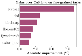
Figure 9: Improvement for fine-grained tasks using SuS.

Appendix I Compute Cost Comparison

We compare the computational requirements of our SuS-X and the baselines in Tab. 14—for each method, we measure the time and memory requirements for one ImageNet class i.e. on 50 test images. For CuPL, VisDesc and SuS-X, we measure the construction time required for curating the enhanced textual prompts and support sets. Note that in practical applications, it is typical to cache the curated support sets/prompts for each class, thereby amortising costs across queries. We note that our SuS-X models offer the most competetive performance-efficiency tradeoff when comparing the compute requirements and accuracy values.

Table 14: Compute requirements of different methods. These numbers are with our tests on a single Nvidia A100-80GB GPU with one ImageNet class i.e. 50 test images.

Method	Construction	Inference	GPU	ImageNet
	Time	Time	Memory	Accuracy
Zero-shot	–	10.22ms	2.2GB	60.32
CALIP	–	121.26ms	24GB	60.57
CLIP+DN	–	10.22ms	2.2GB	60.16
VisDesc	$\sim$3s	10.22ms	2.2GB	59.68
CuPL+e	$\sim$3s	10.22ms	2.2GB	61.64
SuS-X-SD	$\sim$60s	10.50ms	3.2GB	61.84
SuS-X-LC	$\sim$2s	10.50ms	3.2GB	61.89

Appendix J Diversity of CuPL and Photo prompting strategies

In this section, we describe in detail the computation of the diversity metric used in Sec. 4.4.

We assume access to a support set $S$ of size $NC$, where there are $C$ classes and $N$ support samples per class. We denote the support subset of a given class $i$ as $S_{i}=\{s_{i,1},s_{i,2},\dots,s_{i,N}\}$, where $s_{i,j}$ denotes the $j^{th}$ support sample for class $i$. Corresponding to these support subsets, we denote the features of $S_{i}$ as $F_{i}$ (using CLIP’s image encoder):

$$\begin{gathered}F_{i,j}=\texttt{CLIPImageEncoder}(s_{i,j}),F_{i,j}\in\mathbb{R}^{d},i\in[1,C],j\in[1,N]\\ F_{i}=\texttt{Concat}([F_{i,1},F_{i,2},\dots,F_{i,N}]),F_{i}\in\mathbb{R}^{N\times d}\end{gathered}$$

We now compute the mean pairwise cosine similarity between all support samples within a class i.e. for class $i$, we compute:

$$\texttt{PCS}_{i}=\frac{\sum_{j=1}^{N}\sum_{k=1}^{N}F_{i,j}F_{i,k}^{T}}{N^{2}}$$

The intuition is that if all the support samples within a class are similar to each other, then the support set is less diverse. Hence, a higher value of $\texttt{PCS}_{i}$ implies a lower diversity. We then compute the mean PCS over all classes as:

$$\texttt{MPCS}=\frac{\sum_{i=1}^{C}\texttt{PCS}_{i}}{C}$$

Finally, we define diversity to be:

$$\texttt{Diversity}=1-\texttt{MPCS}$$

Appendix K Further Analyses

We conduct some further ablation studies to analyse our novel TIP-X method with more rigour. Due to lack of space in the main paper, we include these ablations here, however these are vital analyses which delineate important properties of our method.

K.1 Contribution of intra-model and inter-modal distances

In Sec. 3.2, we describe our TIP-X method that utilises image-text distances as a bridge for computing image-image intra-modal similarities. We refer to the main equation for computing TIP-X logits again, highlighting the importance of each term:

$$\texttt{TXL}=\underbrace{fW^{T}}_{\text{1. zero-shot component}}+\underbrace{\alpha AL}_{\text{2. intra-modal distance component}}+\underbrace{\gamma\psi(-M)L}_{\text{3. inter-modal distance component}}$$

Zero-shot CLIP utilises only the zero-shot term (1) above. TIP-Adapter utilises the zero-shot and intra-modal distance terms (1+2). Our method uses all three terms (1+2+3). We further ablate this design choice to break down the gains brought forth from each individual term. In Tab. 15, we show the performance gains from each of these terms with our best performing SuS-X-LC model across 19 datasets. We observe large gains from inter-modal and intra-modal distances independently over just using the zero-shot term. Further, both these distances provide complementary information to each other, and hence can be productively combined leading to the best results.

Table 15: Contribution of intra-modal and inter-modal distances.

Dist. terms used	1	1+3	1+2	1+2+3
	(Zero-shot)	(Inter-modal)	(Intra-modal)	(Both)
Average Acc.	52.27	56.30	56.56	56.87
Gain	0	+4.03	+4.29	+4.60

K.2 Comparing name-only SuS-X to few-shot methods

In Sec. 4.1 of the main paper, we showcased SoTA results with our SuS-X model in the name-only setting. Recollect that in this setting, we use no images from the true target distribution. Here, we evaluate how well our SuS-X model fares against methods that use image samples from the true target distribution. We compare our best performing SuS-X-LC method (uses no images from target distribution) with 16-shot TIP-Adapter and 16-shot TIP-X (both using 16 labelled images per class). From Tab. 16, we see that SuS-X-LC is competitive (in green) against these few-shot adaptation methods, despite using no target task images. There are however cases where SuS-X-LC severely underperforms the few-shot methods—this is due to the domain gap between the SuS images and the true labelled images (refer Sec. 4.4).

Table 16: SuS-X against few-shot labelled methods.

Dataset	Zero-shot	SuS-X-LC	TIP-Adapter	TIP-X
		(name-only, ours)	(few-shot)	(few-shot, ours)
ImageNet	60.31	61.89	62.01	62.16
Food101	74.11	77.62	75.82	75.96
OxfordPets	81.82	86.59	84.50	87.52
Caltech101	85.92	89.65	90.43	90.39
Flowers102	62.89	67.97	89.36	90.54
FGVCAircraft	16.71	21.09	29.64	29.61

K.3 Intuitions for best performing configurations

From Tab. 5 of the main paper, we note that our best name-only results are achieved with the LC-Photo and SD-CuPL SuS construction strategies. A natural question arises: “Why do the two SuS construction methods require different prompting strategies for achieving their best results?”. We attempt to answer this question via careful inspection of the support sets curated from these strategies. For this case study, we inspect the support sets for the CIFAR-10 dataset.

(a)

(b)

(c)

(d)

(e)

(f)

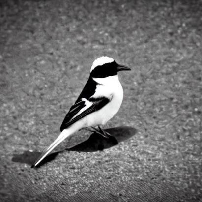
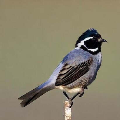
(g)

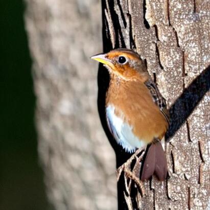
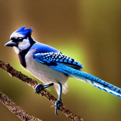
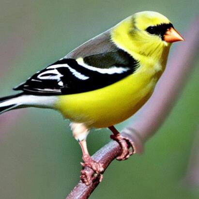
(h)

Figure 10: Uncovering the intuitions for different prompting configurations. We showcase some support samples using different prompting configurations for two CIFAR-10 classes—airplane and bird. The key takeaways upon inspecting these samples are enumerated below.

From Fig. 10, we can draw two key takeaways regarding the best prompting strategies for the two SuS curation methods:

1. LAION-5B retrieval. The support sets constructed with CuPL prompts are largely divergent from the “true” distribution of natural semantic images of the target concepts/classes. This can be noted from the right panels of the first two rows in Fig. 10—this disparity in the retrieved support set images leads to a large domain gap to the target distribution, hence resulting in poorer performance than the Photo prompting strategy. Further, since the LAION-5B support sets consist of natural images i.e. images available on the web, the LAION-5B Photo support set images are closer to the true target distribution of images.

2. Stable Diffusion Generation. The support sets generated using Stable Diffusion represent a synthetic data distribution i.e. there is an innate distribution shift from the target distribution images owing to the target datasets (mostly) consisting of natural images. Hence, the Stable Diffusion support sets are inherently at a disadvantage compared to the LAION-5B support sets. However, within the constructed Stable Diffusion support sets, the CuPL prompting strategy mildly wins over the Photo strategy since it helps generate a more diverse set of images (consisting of more expansive lighting conditions, background scenes etc.)—this diversity helps reduce the domain gap to the target dataset to a small extent. This phenomenon of added diversity in synthetic datasets aiding downstream performance has also been noted in previous works [36].

Appendix L Extended Results on all Datasets

In Tab. 17, we report the accuracies obtained on each of the 19 individual datasets for all our baselines, and our SuS-X model variants with CLIP as te VLM. We also report the average accuracy obtained on the 11 dataset subset used in previous CLIP adaptation works [84, 28, 86]. In Tab. 18, we report all the results with the TCL model as the VLM, and in Tab. 19, we report the results with the BLIP model as the VLM.

Table 17: Training-free zero-shot/name-only results across model configurations and datasets. We report average results using both the 11 dataset subset used by previous works on few-shot adaptation [84, 28, 86] and the entire 19 dataset suite. For the CALIP baseline, we report numbers from the original paper (denoted with a subscript o) as well as our re-implementation (denoted with a subscript (r)). We refer to the Zero-shot CLIP model as ZS-CLIP and CuPL+ensemble baseline as CuPL+e. We use the CuPL+ensemble prompts for CLIP’s text classifier in this experiment. For both variants of our models, we append P or C to the name to distinguish between Photo and CuPL prompt strategies. For instance, SuS-X-LC-P refers to the SuS-X model with LC curation using the Photo strategy. All models use the ResNet-50 visual backbone. The best results for each dataset are bolded and the second best are underlined. This table contains the full set of values used for generating Fig. 4(a) and populating Tab. 2 in the paper.

	UCF101	CIFAR-10	CIFAR-100	Caltech101	Caltech256	ImageNet	SUN397	FGVCAircraft	Birdsnap	StanfordCars	CUB	Flowers102	Food101	OxfordPets	DTD	EuroSAT	ImageNet-Sketch	ImageNet-R	Country211	Average (11 subset)	Average (19 datasets)
ZS-CLIP	55.56	73.10	40.58	85.92	78.98	60.31	59.11	16.71	30.56	56.33	41.31	62.89	74.11	81.82	41.01	26.83	35.42	59.34	13.42	56.41	52.27
CALIPo	61.72	–	–	87.71	–	60.57	58.59	17.76	–	56.27	–	66.38	77.42	86.21	42.39	38.90	–	–	–	59.45	–
CALIPr	55.61	73.15	40.62	86.20	79.08	60.31	59.10	16.71	30.68	56.32	41.40	63.01	74.13	81.84	41.01	26.96	36.10	59.32	13.45	56.47	52.37
CLIP+DN	55.60	74.49	43.73	87.25	79.24	60.16	59.11	17.43	31.23	56.55	43.03	63.32	74.64	81.92	41.21	28.31	35.95	60.37	13.76	56.86	53.02
CuPL	58.97	74.13	42.90	89.29	80.29	61.45	62.55	19.59	35.65	57.28	48.84	65.44	76.94	84.84	48.64	38.38	35.13	61.02	13.27	60.30	55.50
CuPL+e	61.45	74.67	43.35	89.41	80.57	61.64	62.99	19.26	35.80	57.23	48.77	65.93	77.52	85.09	47.45	37.06	35.85	61.17	14.27	60.45	55.76
VisDesc	58.47	73.22	39.69	88.11	79.94	59.68	59.84	16.26	35.65	54.76	48.31	65.37	76.80	82.39	41.96	37.60	33.78	57.16	12.42	58.30	53.76
SuS-X-SD-P	61.72	74.71	44.14	89.65	80.62	61.79	62.96	19.17	36.59	57.37	49.12	67.97	77.59	86.24	49.35	38.11	36.58	62.10	14.26	61.08	56.32
SuS-X-SD-C	61.54	74.69	44.63	89.53	80.64	61.84	62.95	19.47	37.14	57.27	49.12	67.72	77.58	85.34	50.59	45.57	36.30	61.76	14.27	61.76	56.73
SuS-X-LC-P	61.49	74.95	44.48	89.57	80.62	61.89	63.01	21.09	38.50	57.17	48.86	67.07	77.62	86.59	49.23	44.23	37.83	62.10	14.24	61.72	56.87
SuS-X-LC-C	61.43	74.76	44.12	89.61	80.63	61.79	62.94	20.34	37.07	57.06	48.86	67.60	77.58	85.22	49.47	37.16	36.45	61.39	14.26	60.93	56.20

Table 18: Training-free zero-shot/name-only results across model configurations using the TCL [76] architecture. For our SuS-X models, we only use the two best configurations from the previous CLIP experiment i.e. SuS-X-SD with CuPL strategy and SuS-X-LC with Photo strategy. This table contains the full set of values used for populating Tab. 3 in the paper.

	UCF101	CIFAR-10	CIFAR-100	Caltech101	Caltech256	ImageNet	SUN397	FGVCAircraft	Birdsnap	StanfordCars	CUB	Flowers102	Food101	OxfordPets	DTD	EuroSAT	ImageNet-Sketch	ImageNet-R	Country211	Average (11 subset)	Average (19 datasets)
ZS-TCL	35.29	82.33	50.86	77.65	61.90	35.55	42.12	2.25	4.51	1.53	7.63	28.30	24.71	20.63	28.55	20.80	24.24	46.05	1.42	28.84	31.38
CuPL	41.23	81.75	52.63	81.66	65.91	41.60	49.35	3.48	6.83	2.11	10.20	26.10	23.62	22.15	42.84	26.30	25.67	53.61	4.07	32.77	34.79
CuPL+e	41.63	82.07	52.66	81.29	66.46	41.36	49.98	3.51	6.60	2.11	9.80	26.91	24.84	21.17	41.96	25.88	26.36	53.36	3.68	34.82	32.79
VisDesc	42.53	82.30	51.89	77.00	66.51	40.40	51.18	3.21	5.69	2.91	8.96	25.13	27.16	24.58	34.28	21.27	27.05	49.26	3.57	31.77	33.94
SuS-X-SD-C	47.66	82.92	55.19	81.38	66.52	52.29	49.98	9.21	13.60	2.31	9.72	30.98	48.87	65.96	48.17	28.75	32.22	58.95	3.66	42.32	41.49
SuS-X-LC-P	50.28	83.14	57.47	81.38	66.80	52.77	49.97	10.98	17.93	2.57	9.77	30.04	48.06	69.96	46.63	36.90	36.28	57.58	3.72	43.59	42.75
												*We use the official TCL-base checkpoint from here for these results.

Table 19: Training-free zero-shot/name-only results across model configurations using the BLIP [46] architecture. For our SuS-X models, we only use the two best configurations from the previous CLIP experiment i.e. SuS-X-SD with CuPL strategy and SuS-X-LC with Photo strategy. This table contains the full set of values used for populating Tab. 3 in the paper.

	UCF101	CIFAR-10	CIFAR-100	Caltech101	Caltech256	ImageNet	SUN397	FGVCAircraft	Birdsnap	StanfordCars	CUB	Flowers102	Food101	OxfordPets	DTD	EuroSAT	ImageNet-Sketch	ImageNet-R	Country211	Average (11 subset)	Average (19 datasets)
ZS-BLIP	50.49	86.68	61.72	92.13	82.17	50.59	54.22	5.40	10.21	54.71	14.95	40.15	54.21	59.04	44.68	44.10	43.69	70.93	5.84	49.97	48.73
CuPL	56.09	86.06	61.99	92.41	83.45	52.96	59.16	5.85	12.24	54.64	18.53	43.97	56.14	72.00	52.95	39.37	44.83	72.27	6.26	53.23	51.11
CuPL+e	55.61	86.33	62.16	92.29	83.59	53.07	59.38	6.27	12.18	54.89	18.63	43.72	57.10	71.73	53.30	41.48	45.34	72.40	6.42	53.53	51.36
VisDesc	53.42	86.78	60.47	92.04	81.53	50.94	55.85	6.30	11.69	54.64	16.65	42.71	58.50	69.22	47.45	42.25	43.30	68.62	6.01	52.12	49.91
SuS-X-SD-C	57.28	87.56	63.60	92.33	83.66	55.93	59.46	10.14	16.95	54.89	18.95	44.38	62.75	74.68	56.15	45.36	46.51	73.85	6.45	55.76	53.20
SuS-X-LC-P	59.90	88.28	64.43	92.29	83.61	56.75	59.39	11.82	23.78	54.94	19.24	43.97	64.14	79.72	55.91	51.62	48.53	73.42	6.44	57.31	54.64
												*We use the official BLIP-base checkpoint from here for these results.

Appendix M Results with different Visual Backbones

All our main results use the ResNet-50 [35] visual backbone for CLIP’s image encoder. In Tab. 20, we compare the accuracies obtained on all 19 datasets using 2 different visual backbone model classes—ResNets [35] (ResNet-50, ResNet-101) and Vision Transformers [22] (ViT-B/32, ViT-B/16). We observe that the accuracy values monotonically improve as we increase the model capacity.

Table 20: Training-free name-only results across visual backbones. For this experiment, we use the default versions of our SuS-X models: SuS-X-LC with Photo strategy and SuS-X-SD with CuPL strategy. This experiment uses the CuPL prompts for CLIP’s text classifier. This table contains the raw data for generating Fig. 4(c) of the paper.

		UCF101	CIFAR-10	CIFAR-100	Caltech101	Caltech256	ImageNet	SUN397	FGVCAircraft	Birdsnap	StanfordCars	CUB	Flowers102	Food101	OxfordPets	DTD	EuroSAT	ImageNet-Sketch	ImageNet-R	Country211	Average (11 subset)	Average (19 datasets)
RN50	SuS-X-LC	59.98	74.79	44.22	89.29	80.29	61.66	62.70	21.87	38.56	56.92	48.90	66.91	77.21	86.35	50.06	43.99	37.25	61.97	13.21	61.54	56.64
	SuS-X-SD	59.48	74.21	44.33	89.25	80.27	61.65	62.58	19.92	37.00	57.14	49.10	67.32	77.02	85.09	51.00	47.69	37.25	61.73	13.30	61.65	56.59
RN101	SuS-X-LC	60.03	77.51	46.72	92.09	81.96	62.11	61.50	22.92	39.87	61.20	45.82	59.28	78.52	88.44	51.18	39.23	40.05	69.07	11.45	61.50	57.31
	SuS-X-SD	57.84	76.97	46.01	92.09	81.96	62.18	61.61	21.66	35.60	61.05	45.93	60.90	78.41	86.56	51.95	39.23	40.47	68.94	11.41	61.23	56.88
ViT-B/32	SuS-X-LC	63.49	89.32	65.25	93.18	84.73	64.73	65.49	23.01	40.77	61.19	53.03	68.01	80.31	87.95	52.25	53.91	43.10	70.55	14.91	64.87	61.85
	SuS-X-SD	63.20	88.39	64.84	93.18	84.73	64.71	65.47	21.66	38.97	61.12	53.52	68.17	80.24	86.81	51.89	53.91	43.27	70.42	14.91	64.58	61.55
ViT-B/16	SuS-X-LC	66.72	90.94	68.66	93.91	87.41	70.00	67.85	30.51	47.71	65.90	56.96	73.08	86.08	91.58	55.32	58.06	49.34	78.20	19.19	69.00	66.18
	SuS-X-SD	66.59	89.88	68.47	93.96	87.45	69.88	67.73	28.68	45.53	66.13	57.11	73.81	86.08	90.57	54.55	57.49	49.51	78.22	19.28	68.68	65.84

Appendix N Results with different Text-to-Image Generation Models

We also experiment with different text-to-image generation models for support set generation to showcase the generalisability and robustness of our method’s results. Tab. 21 depicts SuS-X-SD results by generating support sets using different text-to-image generation models. The results presented in the main paper all use the Stable-Diffusion-v1.4 model, but we also note similar gains across three other generative models.

Table 21: SuS-X-SD Results with additional T2I models.

T2I Model	ImageNet	EuroSAT	DTD	OxfordPets	Average
ZS-CLIP (baseline)	60.31	26.83	41.01	81.82	52.49
StableDiffusion-1.4 (from main paper)	61.84	45.57	50.59	85.34	60.84 (+8.35%)
Kandinsky2.1	61.83	44.96	49.17	85.47	60.36 (+7.87%)
OpenJourney-4	61.81	45.00	50.71	85.17	60.67 (+8.18%)
Protogen-2.2	61.82	48.67	50.35	85.26	61.52 (+9.03%)

Appendix O Fine-tuning SuS-X

Despite our work’s main focus being the training-free adaptation regime, we explore some preliminary results with fine-tuning SuS-X on a few datasets. We compare both the training-free and the fine-tuned variants of SuS-X with other CLIP adaptation methods that use full or partial (parameter-efficient fine-tuning) in Tab. 22. We note for some datasets, full/partial fine-tuning methods perform better than training-free SuS-X. However, due to the domain gap between StableDiffusion/LAION-5B curated data and real test data, the gains are not large (confirming prior work [36, sariyildiz2023fake]). Further, we note that full fine-tuning and SuS-X are complementary, allowing a large boost in performance for SuS-X-F. On the other hand, we emphasise that the goal of our work is to keep the approach flexible and scalable—one can apply SuS-X to an arbitrary number of rare categories without training. This training-free approach can particularly benefit when the categories of interest vary frequently, rendering repetitive fine-tuning inefficient. Moreover, fine-tuning forces the model to fit a very specific task distribution, enforcing forgetting of the model’s pre-trained performance on a wide array of tasks. Since SuS-X only requires target task class names and does not fine-tune the model, we can cache the task-specific support sets a-priori and switch them dynamically based on the task at hand, without causing catastrophic forgetting of CLIP’s pre-trained knowledge.

Table 22: Fine-tuning methods vs SuS-X.

Method	ZS-CLIP	FT-CLIP	CoOp [88]	CLIP-Adapter [28]	SuS-X	SuS-X-F
	(No adaptation)	(Full fine-tuning)	(PromptTuning)	(Adapters)	(Ours)	(Ours)
ImageNet	60.31	60.35	60.96	61.61	61.89	63.22
EuroSAT	26.83	55.37	52.12	57.00	44.23	59.22
DTD	41.01	50.35	45.66	49.29	49.23	52.30
OxfordPets	81.82	84.51	85.99	85.06	86.59	87.77

References

- [1] Jean-Baptiste Alayrac, Jeff Donahue, Pauline Luc, Antoine Miech, Iain Barr, Yana Hasson, Karel Lenc, Arthur Mensch, Katie Millican, Malcolm Reynolds, et al. Flamingo: a visual language model for few-shot learning. arXiv preprint arXiv:2204.14198, 2022.
- [2] Max Bain, Arsha Nagrani, Gül Varol, and Andrew Zisserman. A clip-hitchhiker’s guide to long video retrieval. arXiv preprint arXiv:2205.08508, 2022.
- [3] Manuele Barraco, Marcella Cornia, Silvia Cascianelli, Lorenzo Baraldi, and Rita Cucchiara. The unreasonable effectiveness of clip features for image captioning: An experimental analysis. In Proceedings of the IEEE/CVF Conference on Computer Vision and Pattern Recognition, pages 4662–4670, 2022.
- [4] Sara Beery, Grant Van Horn, and Pietro Perona. Recognition in terra incognita. In Proceedings of the European conference on computer vision (ECCV), pages 456–473, 2018.
- [5] Thomas Berg, Jiongxin Liu, Seung Woo Lee, Michelle L Alexander, David W Jacobs, and Peter N Belhumeur. Birdsnap: Large-scale fine-grained visual categorization of birds. In Proceedings of the IEEE Conference on Computer Vision and Pattern Recognition, pages 2011–2018, 2014.
- [6] Rishi Bommasani, Drew A Hudson, Ehsan Adeli, Russ Altman, Simran Arora, Sydney von Arx, Michael S Bernstein, Jeannette Bohg, Antoine Bosselut, Emma Brunskill, et al. On the opportunities and risks of foundation models. arXiv preprint arXiv:2108.07258, 2021.
- [7] Lukas Bossard, Matthieu Guillaumin, and Luc Van Gool. Food-101–mining discriminative components with random forests. In European conference on computer vision, pages 446–461. Springer, 2014.
- [8] Tom Brown, Benjamin Mann, Nick Ryder, Melanie Subbiah, Jared D Kaplan, Prafulla Dhariwal, Arvind Neelakantan, Pranav Shyam, Girish Sastry, Amanda Askell, et al. Language models are few-shot learners. Advances in neural information processing systems, 33:1877–1901, 2020.
- [9] Jacob Browning and Yann Lecun. Ai and the limits of language, 2022.
- [10] Adrian Bulat and Georgios Tzimiropoulos. Language-aware soft prompting for vision & language foundation models. arXiv preprint arXiv:2210.01115, 2022.
- [11] Delong Chen, Zhao Wu, Fan Liu, Zaiquan Yang, Yixiang Huang, Yiping Bao, and Erjin Zhou. Prototypical contrastive language image pretraining. arXiv preprint arXiv:2206.10996, 2022.
- [12] Guangyi Chen, Weiran Yao, Xiangchen Song, Xinyue Li, Yongming Rao, and Kun Zhang. Prompt learning with optimal transport for vision-language models. arXiv preprint arXiv:2210.01253, 2022.
- [13] Gordon Christie, Neil Fendley, James Wilson, and Ryan Mukherjee. Functional map of the world. In Proceedings of the IEEE Conference on Computer Vision and Pattern Recognition, pages 6172–6180, 2018.
- [14] Mircea Cimpoi, Subhransu Maji, Iasonas Kokkinos, Sammy Mohamed, and Andrea Vedaldi. Describing textures in the wild. In Proceedings of the IEEE conference on computer vision and pattern recognition, pages 3606–3613, 2014.
- [15] Nigel H Collier, Fangyu Liu, and Ehsan Shareghi. On reality and the limits of language data. arXiv preprint arXiv:2208.11981, 2022.
- [16] Andrea Cossu, Tinne Tuytelaars, Antonio Carta, Lucia Passaro, Vincenzo Lomonaco, and Davide Bacciu. Continual pre-training mitigates forgetting in language and vision. arXiv preprint arXiv:2205.09357, 2022.
- [17] Guillaume Couairon, Matthijs Douze, Matthieu Cord, and Holger Schwenk. Embedding arithmetic of multimodal queries for image retrieval. In Proceedings of the IEEE/CVF Conference on Computer Vision and Pattern Recognition, pages 4950–4958, 2022.
- [18] Jia Deng, Wei Dong, Richard Socher, Li-Jia Li, Kai Li, and Li Fei-Fei. Imagenet: A large-scale hierarchical image database. In 2009 IEEE conference on computer vision and pattern recognition, pages 248–255. Ieee, 2009.
- [19] Mohammad Mahdi Derakhshani, Enrique Sanchez, Adrian Bulat, Victor Guilherme Turrisi da Costa, Cees GM Snoek, Georgios Tzimiropoulos, and Brais Martinez. Variational prompt tuning improves generalization of vision-language models. arXiv preprint arXiv:2210.02390, 2022.
- [20] Karan Desai and Justin Johnson. Virtex: Learning visual representations from textual annotations. In Proceedings of the IEEE/CVF conference on computer vision and pattern recognition, pages 11162–11173, 2021.
- [21] Kun Ding, Ying Wang, Pengzhang Liu, Qiang Yu, Haojian Zhang, Shiming Xiang, and Chunhong Pan. Prompt tuning with soft context sharing for vision-language models. arXiv preprint arXiv:2208.13474, 2022.
- [22] Alexey Dosovitskiy, Lucas Beyer, Alexander Kolesnikov, Dirk Weissenborn, Xiaohua Zhai, Thomas Unterthiner, Mostafa Dehghani, Matthias Minderer, Georg Heigold, Sylvain Gelly, et al. An image is worth 16x16 words: Transformers for image recognition at scale. arXiv preprint arXiv:2010.11929, 2020.
- [23] Yu Du, Fangyun Wei, Zihe Zhang, Miaojing Shi, Yue Gao, and Guoqi Li. Learning to prompt for open-vocabulary object detection with vision-language model. In Proceedings of the IEEE/CVF Conference on Computer Vision and Pattern Recognition, pages 14084–14093, 2022.
- [24] Alex Fang, Gabriel Ilharco, Mitchell Wortsman, Yuhao Wan, Vaishaal Shankar, Achal Dave, and Ludwig Schmidt. Data determines distributional robustness in contrastive language image pre-training (clip). arXiv preprint arXiv:2205.01397, 2022.
- [25] Li Fei-Fei, Rob Fergus, and Pietro Perona. Learning generative visual models from few training examples: An incremental bayesian approach tested on 101 object categories. In 2004 conference on computer vision and pattern recognition workshop, pages 178–178. IEEE, 2004.
- [26] Robert Fergus, Li Fei-Fei, Pietro Perona, and Andrew Zisserman. Learning object categories from google’s image search. In Tenth IEEE International Conference on Computer Vision (ICCV’05) Volume 1, volume 2, pages 1816–1823. IEEE, 2005.
- [27] Benjamin Feuer, Ameya Joshi, and Chinmay Hegde. Caption supervision enables robust learners. arXiv preprint arXiv:2210.07396, 2022.
- [28] Peng Gao, Shijie Geng, Renrui Zhang, Teli Ma, Rongyao Fang, Yongfeng Zhang, Hongsheng Li, and Yu Qiao. Clip-adapter: Better vision-language models with feature adapters. arXiv preprint arXiv:2110.04544, 2021.
- [29] Yuting Gao, Jinfeng Liu, Zihan Xu, Jun Zhang, Ke Li, and Chunhua Shen. Pyramidclip: Hierarchical feature alignment for vision-language model pretraining. arXiv preprint arXiv:2204.14095, 2022.
- [30] Golnaz Ghiasi, Xiuye Gu, Yin Cui, and Tsung-Yi Lin. Open-vocabulary image segmentation. arXiv preprint arXiv:2112.12143, 2021.
- [31] Shashank Goel, Hritik Bansal, Sumit Bhatia, Ryan Rossi, Vishwa Vinay, and Aditya Grover. Cyclip: Cyclic contrastive language-image pretraining. arXiv preprint arXiv:2205.14459, 2022.
- [32] Gregory Griffin, Alex Holub, and Pietro Perona. Caltech-256 object category dataset. 2007.
- [33] Xiuye Gu, Tsung-Yi Lin, Weicheng Kuo, and Yin Cui. Open-vocabulary object detection via vision and language knowledge distillation. arXiv preprint arXiv:2104.13921, 2021.
- [34] Ziyu Guo, Renrui Zhang, Longtian Qiu, Xianzheng Ma, Xupeng Miao, Xuming He, and Bin Cui. Calip: Zero-shot enhancement of clip with parameter-free attention. arXiv preprint arXiv:2209.14169, 2022.
- [35] Kaiming He, Xiangyu Zhang, Shaoqing Ren, and Jian Sun. Deep residual learning for image recognition. In Proceedings of the IEEE conference on computer vision and pattern recognition, pages 770–778, 2016.
- [36] Ruifei He, Shuyang Sun, Xin Yu, Chuhui Xue, Wenqing Zhang, Philip Torr, Song Bai, and Xiaojuan Qi. Is synthetic data from generative models ready for image recognition? arXiv preprint arXiv:2210.07574, 2022.
- [37] Patrick Helber, Benjamin Bischke, Andreas Dengel, and Damian Borth. Eurosat: A novel dataset and deep learning benchmark for land use and land cover classification. IEEE Journal of Selected Topics in Applied Earth Observations and Remote Sensing, 12(7):2217–2226, 2019.
- [38] Dan Hendrycks, Steven Basart, Norman Mu, Saurav Kadavath, Frank Wang, Evan Dorundo, Rahul Desai, Tyler Zhu, Samyak Parajuli, Mike Guo, et al. The many faces of robustness: A critical analysis of out-of-distribution generalization. In Proceedings of the IEEE/CVF International Conference on Computer Vision, pages 8340–8349, 2021.
- [39] Jonathan Ho and Tim Salimans. Classifier-free diffusion guidance. arXiv preprint arXiv:2207.12598, 2022.
- [40] Tony Huang, Jack Chu, and Fangyun Wei. Unsupervised prompt learning for vision-language models. arXiv preprint arXiv:2204.03649, 2022.
- [41] Chao Jia, Yinfei Yang, Ye Xia, Yi-Ting Chen, Zarana Parekh, Hieu Pham, Quoc Le, Yun-Hsuan Sung, Zhen Li, and Tom Duerig. Scaling up visual and vision-language representation learning with noisy text supervision. In International Conference on Machine Learning, pages 4904–4916. PMLR, 2021.
- [42] Daniel S Kermany, Michael Goldbaum, Wenjia Cai, Carolina CS Valentim, Huiying Liang, Sally L Baxter, Alex McKeown, Ge Yang, Xiaokang Wu, Fangbing Yan, et al. Identifying medical diagnoses and treatable diseases by image-based deep learning. Cell, 172(5):1122–1131, 2018.
- [43] Jonathan Krause, Michael Stark, Jia Deng, and Li Fei-Fei. 3d object representations for fine-grained categorization. In Proceedings of the IEEE international conference on computer vision workshops, pages 554–561, 2013.
- [44] Alex Krizhevsky, Geoffrey Hinton, et al. Learning multiple layers of features from tiny images. 2009.
- [45] Christoph H Lampert, Hannes Nickisch, and Stefan Harmeling. Learning to detect unseen object classes by between-class attribute transfer. In 2009 IEEE conference on computer vision and pattern recognition, pages 951–958. IEEE, 2009.
- [46] Junnan Li, Dongxu Li, Caiming Xiong, and Steven Hoi. Blip: Bootstrapping language-image pre-training for unified vision-language understanding and generation. arXiv preprint arXiv:2201.12086, 2022.
- [47] Yangguang Li, Feng Liang, Lichen Zhao, Yufeng Cui, Wanli Ouyang, Jing Shao, Fengwei Yu, and Junjie Yan. Supervision exists everywhere: A data efficient contrastive language-image pre-training paradigm. arXiv preprint arXiv:2110.05208, 2021.
- [48] Weixin Liang, Yuhui Zhang, Yongchan Kwon, Serena Yeung, and James Zou. Mind the gap: Understanding the modality gap in multi-modal contrastive representation learning. arXiv preprint arXiv:2203.02053, 2022.
- [49] Yuning Lu, Jianzhuang Liu, Yonggang Zhang, Yajing Liu, and Xinmei Tian. Prompt distribution learning. arXiv preprint arXiv:2205.03340, 2022.
- [50] Yiwei Ma, Guohai Xu, Xiaoshuai Sun, Ming Yan, Ji Zhang, and Rongrong Ji. X-clip: End-to-end multi-grained contrastive learning for video-text retrieval. arXiv preprint arXiv:2207.07285, 2022.
- [51] Subhransu Maji, Esa Rahtu, Juho Kannala, Matthew Blaschko, and Andrea Vedaldi. Fine-grained visual classification of aircraft. arXiv preprint arXiv:1306.5151, 2013.
- [52] Shu Manli, Nie Weili, Huang De-An, Yu Zhiding, Goldstein Tom, Anandkumar Anima, and Xiao Chaowei. Test-time prompt tuning for zero-shot generalization in vision-language models. In NeurIPS, 2022.
- [53] Sachit Menon and Carl Vondrick. Visual classification via description from large language models. arXiv preprint arXiv:2210.07183, 2022.
- [54] Ron Mokady, Amir Hertz, and Amit H Bermano. Clipcap: Clip prefix for image captioning. arXiv preprint arXiv:2111.09734, 2021.
- [55] Thao Nguyen, Gabriel Ilharco, Mitchell Wortsman, Sewoong Oh, and Ludwig Schmidt. Quality not quantity: On the interaction between dataset design and robustness of clip. arXiv preprint arXiv:2208.05516, 2022.
- [56] Maria-Elena Nilsback and Andrew Zisserman. Automated flower classification over a large number of classes. In 2008 Sixth Indian Conference on Computer Vision, Graphics & Image Processing, pages 722–729. IEEE, 2008.
- [57] Zachary Novack, Saurabh Garg, Julian McAuley, and Zachary C Lipton. Chils: Zero-shot image classification with hierarchical label sets. arXiv preprint arXiv:2302.02551, 2023.
- [58] Omiros Pantazis, Gabriel Brostow, Kate Jones, and Oisin Mac Aodha. Svl-adapter: Self-supervised adapter for vision-language pretrained models. arXiv preprint arXiv:2210.03794, 2022.
- [59] Omkar M Parkhi, Andrea Vedaldi, Andrew Zisserman, and CV Jawahar. Cats and dogs. In 2012 IEEE conference on computer vision and pattern recognition, pages 3498–3505. IEEE, 2012.
- [60] Sarah Pratt, Rosanne Liu, and Ali Farhadi. What does a platypus look like? generating customized prompts for zero-shot image classification. arXiv preprint arXiv:2209.03320, 2022.
- [61] Alec Radford, Jong Wook Kim, Chris Hallacy, Aditya Ramesh, Gabriel Goh, Sandhini Agarwal, Girish Sastry, Amanda Askell, Pamela Mishkin, Jack Clark, et al. Learning transferable visual models from natural language supervision. In International Conference on Machine Learning, pages 8748–8763. PMLR, 2021.
- [62] Aditya Ramesh, Prafulla Dhariwal, Alex Nichol, Casey Chu, and Mark Chen. Hierarchical text-conditional image generation with clip latents. arXiv preprint arXiv:2204.06125, 2022.
- [63] Robin Rombach, Andreas Blattmann, Dominik Lorenz, Patrick Esser, and Bjarn Ommer. High-resolution image synthesis with latent diffusion models. In Proceedings of the IEEE Conference on Computer Vision and Pattern Recognition (CVPR), 2022.
- [64] Shibani Santurkar, Yann Dubois, Rohan Taori, Percy Liang, and Tatsunori Hashimoto. Is a caption worth a thousand images? a controlled study for representation learning. arXiv preprint arXiv:2207.07635, 2022.
- [65] Christoph Schuhmann, Romain Beaumont, Richard Vencu, Cade Gordon, Ross Wightman, Mehdi Cherti, Theo Coombes, Aarush Katta, Clayton Mullis, Mitchell Wortsman, et al. Laion-5b: An open large-scale dataset for training next generation image-text models. arXiv preprint arXiv:2210.08402, 2022.
- [66] Gyungin Shin, Weidi Xie, and Samuel Albanie. Namedmask: Distilling segmenters from complementary foundation models. arXiv preprint arXiv:2209.11228, 2022.
- [67] Gyungin Shin, Weidi Xie, and Samuel Albanie. Reco: Retrieve and co-segment for zero-shot transfer. arXiv preprint arXiv:2206.07045, 2022.
- [68] Khurram Soomro, Amir Roshan Zamir, and Mubarak Shah. Ucf101: A dataset of 101 human actions classes from videos in the wild. arXiv preprint arXiv:1212.0402, 2012.
- [69] Tejas Srinivasan, Ting-Yun Chang, Leticia Leonor Pinto Alva, Georgios Chochlakis, Mohammad Rostami, and Jesse Thomason. Climb: A continual learning benchmark for vision-and-language tasks. arXiv preprint arXiv:2206.09059, 2022.
- [70] Vishaal Udandarao. Understanding and Fixing the Modality Gap in Vision-Language Models. Master’s thesis, University of Cambridge, 2022.
- [71] Vishaal Udandarao, Abhishek Maiti, Deepak Srivatsav, Suryatej Reddy Vyalla, Yifang Yin, and Rajiv Ratn Shah. Cobra: Contrastive bi-modal representation algorithm. arXiv preprint arXiv:2005.03687, 2020.
- [72] Catherine Wah, Steve Branson, Peter Welinder, Pietro Perona, and Serge Belongie. The caltech-ucsd birds-200-2011 dataset. 2011.
- [73] Haohan Wang, Songwei Ge, Zachary Lipton, and Eric P Xing. Learning robust global representations by penalizing local predictive power. In Advances in Neural Information Processing Systems, pages 10506–10518, 2019.
- [74] Zirui Wang, Jiahui Yu, Adams Wei Yu, Zihang Dai, Yulia Tsvetkov, and Yuan Cao. Simvlm: Simple visual language model pretraining with weak supervision. arXiv preprint arXiv:2108.10904, 2021.
- [75] Jianxiong Xiao, James Hays, Krista A Ehinger, Aude Oliva, and Antonio Torralba. Sun database: Large-scale scene recognition from abbey to zoo. In 2010 IEEE computer society conference on computer vision and pattern recognition, pages 3485–3492. IEEE, 2010.
- [76] Jinyu Yang, Jiali Duan, Son Tran, Yi Xu, Sampath Chanda, Liqun Chen, Belinda Zeng, Trishul Chilimbi, and Junzhou Huang. Vision-language pre-training with triple contrastive learning. In Proceedings of the IEEE/CVF Conference on Computer Vision and Pattern Recognition, pages 15671–15680, 2022.
- [77] Lewei Yao, Runhui Huang, Lu Hou, Guansong Lu, Minzhe Niu, Hang Xu, Xiaodan Liang, Zhenguo Li, Xin Jiang, and Chunjing Xu. Filip: Fine-grained interactive language-image pre-training. arXiv preprint arXiv:2111.07783, 2021.
- [78] Haoxuan You, Luowei Zhou, Bin Xiao, Noel Codella, Yu Cheng, Ruochen Xu, Shih-Fu Chang, and Lu Yuan. Learning visual representation from modality-shared contrastive language-image pre-training. arXiv preprint arXiv:2207.12661, 2022.
- [79] Jiahui Yu, Zirui Wang, Vijay Vasudevan, Legg Yeung, Mojtaba Seyedhosseini, and Yonghui Wu. Coca: Contrastive captioners are image-text foundation models. arXiv preprint arXiv:2205.01917, 2022.
- [80] Youngjae Yu, Jiwan Chung, Heeseung Yun, Jack Hessel, JaeSung Park, Ximing Lu, Prithviraj Ammanabrolu, Rowan Zellers, Ronan Le Bras, Gunhee Kim, et al. Multimodal knowledge alignment with reinforcement learning. arXiv preprint arXiv:2205.12630, 2022.
- [81] Renrui Zhang, Rongyao Fang, Peng Gao, Wei Zhang, Kunchang Li, Jifeng Dai, Yu Qiao, and Hongsheng Li. Tip-adapter: Training-free clip-adapter for better vision-language modeling. arXiv preprint arXiv:2111.03930, 2021.
- [82] Renrui Zhang, Xiangfei Hu, Bohao Li, Siyuan Huang, Hanqiu Deng, Hongsheng Li, Yu Qiao, and Peng Gao. Prompt, generate, then cache: Cascade of foundation models makes strong few-shot learners. arXiv preprint arXiv:2303.02151, 2023.
- [83] Renrui Zhang, Longtian Qiu, Wei Zhang, and Ziyao Zeng. Vt-clip: Enhancing vision-language models with visual-guided texts. arXiv preprint arXiv:2112.02399, 2021.
- [84] Renrui Zhang, Wei Zhang, Rongyao Fang, Peng Gao, Kunchang Li, Jifeng Dai, Yu Qiao, and Hongsheng Li. Tip-adapter: Training-free adaption of clip for few-shot classification. arXiv preprint arXiv:2207.09519, 2022.
- [85] Yuhao Zhang, Hang Jiang, Yasuhide Miura, Christopher D Manning, and Curtis P Langlotz. Contrastive learning of medical visual representations from paired images and text. arXiv preprint arXiv:2010.00747, 2020.
- [86] Kaiyang Zhou, Jingkang Yang, Chen Change Loy, and Ziwei Liu. Learning to prompt for vision-language models. arXiv preprint arXiv:2109.01134, 2021.
- [87] Kaiyang Zhou, Jingkang Yang, Chen Change Loy, and Ziwei Liu. Conditional prompt learning for vision-language models. arXiv preprint arXiv:2203.05557, 2022.
- [88] Kaiyang Zhou, Jingkang Yang, Chen Change Loy, and Ziwei Liu. Learning to prompt for vision-language models. International Journal of Computer Vision, 130(9):2337–2348, 2022.
- [89] Yifei Zhou, Juntao Ren, Fengyu Li, Ramin Zabih, and Ser-Nam Lim. Distribution normalization: An “effortless” test-time augmentation for contrastively learned visual-language models. arXiv preprint arXiv:2302.11084, 2023.