Cubic fixed point in three dimensions: Monte Carlo simulations of the $\phi^{4}$ model on the lattice

Abstract

We study the cubic fixed point for $N=3$ and $4$ by using finite-size scaling applied to data obtained from Monte Carlo simulations of the $N$-component $\phi^{4}$ model on the simple cubic lattice. We generalize the idea of improved models to a two-parameter family of models. The two-parameter space is scanned for the point, where the amplitudes of the two leading corrections to scaling vanish. To this end, a dimensionless quantity is introduced that monitors the breaking of the $O(N)$ invariance. For $N=4$, we determine the correction exponents $\omega_{1}=0.763(24)$ and $\omega_{2}=0.082(5)$. In the case of $N=3$, we obtain $Y_{4}=0.0142(6)$ for the renormalization group exponent of the cubic perturbation at the $O(3)$-invariant fixed point, while the correction exponent $\omega_{2}=0.0133(8)$ at the cubic fixed point. Simulations close to the improved point result in the estimates $\nu=0.7202(7)$ and $\eta=0.0371(2)$ of the critical exponents of the cubic fixed point for $N=4$. For $N=3$, at the cubic fixed point, the $O(3)$ symmetry is only mildly broken and the critical exponents differ only by little from those of the $O(3)$-invariant fixed point. We find $-0.00001\lessapprox\eta_{cubic}-\eta_{O(3)}\lessapprox 0.00007$ and $\nu_{cubic}-\nu_{O(3)}=-0.00061(10)$.

I Introduction

The three-dimensional Heisenberg universality class is supposed to describe the critical behavior of isotropic magnets, for example, the Curie transition in isotropic ferromagnets such as Ni and EuO, and of antiferromagnets such as RbMnF3 at the Néel transition point. For a more detailed discussion, see for instance Sec. 5 of PeVi02 or the introduction of Ref. ourHeisen . The Heisenberg universality class is characterized by an $O(3)$ symmetry of the order parameter. Due to the crystal structure, in real systems, one expects that there are weak interactions that break the $O(3)$ symmetry and possess only cubic symmetry. Therefore, it is important to study the effect of such perturbations theoretically. This has been done by using field-theoretic methods for five decades now. In their seminal paper on the $\epsilon$ expansion WiFi72 , Wilson and Fisher discuss the problem to the leading order for $O(2)$ symmetry. Very soon the problem was taken on by various authors generalizing the calculation to $O(N)$ symmetry with arbitrary $N$ and extending the calculation to higher orders in the $\epsilon$ expansion. For example, in 1973, Aharony Aha73 performed the calculation to two-loop order. Furthermore, large-$N$ expansions around decoupled Ising systems were performed. See Ref. Aha73Lett and recently DBinder .

It is beyond the scope of this paper to give a detailed account of the progress that has been made over the years. The development up to and the state of the art in 1999 is nicely summarized in Ref. Carmona . See also Refs. Varna00 ; Folk00 . At that time, the $\epsilon$ expansion had been computed up to five loop Frohlinde and the expansion in three dimensions fixed up to six loop Carmona .

Here we like to summarize some basic facts to set the scene for our numerical study. We follow the book Cardy . Similar discussions can be found in other reviews on the subject. The reduced Hamiltonian of the $\phi^{4}$ theory with two quartic couplings in the continuum is given by, [see, for example, Eq. (5.66) of Ref. Cardy ]

$${\cal H}=\int\mbox{d}^{d}x\left\{\frac{1}{2}\sum_{i=1}^{N}[(\partial_{\mu}\phi_{i})^{2}+r\phi_{i}^{2}]+\sum_{i,j=1}^{N}(u+v\delta_{ij})\phi_{i}^{2}\phi_{j}^{2}\right\}\;,$$ (1)

where $\phi_{i}$ is a real number. Note that for $d=4-\epsilon$, $\epsilon>0$ and $\epsilon$ small, these $\phi^{4}$ terms are the only relevant perturbations of the free (or Gaussian) theory. For $v=0$ the system is $O(N)$-invariant. The question is, whether the term that breaks this invariance is relevant at the $O(N)$-invariant fixed point. The qualitative picture already emerges from the leading-order calculation of the $\epsilon$ expansion. It can be obtained from the renormalization group (RG) flow on the critical surface [Eqs. (2)] taken from Eqs. (5.67) and (5.68) of Ref. Cardy :

$$\frac{\mbox{d}u}{\mbox{d}l} = \epsilon u-8(N+8)u^{2}-48uv+...\;,$$

$$\frac{\mbox{d}v}{\mbox{d}l} = \epsilon v-96uv-72v^{2}+...\;,$$ (2)

where $l$ is the logarithm of a length scale. The set of differential equations (2) has four fixed points Cardy :

• Gaussian fixed point $(u,v)=(0,0)$ ;

• Decoupled Ising fixed point $(u,v)=(0,\epsilon/72)$ ;

• $O(N)$-invariant fixed point $(u,v)=(\epsilon/(8(N+8)),0)$ ;

• Cubic fixed point $(u,v)=(\epsilon/(24N),(N-4)\epsilon/(72N))$ .

The Gaussian and the decoupled Ising fixed points are always unstable. Whether the $O(N)$-invariant or the cubic fixed point is stable depends on $N$. For $N>N_{c}$, the cubic fixed point is stable, while for $N<N_{c}$ it is the $O(N)$-invariant fixed point. At one loop, setting $\epsilon=1$, $N_{c}=4$. Analyzing higher orders in the $\epsilon$ expansion, $N_{c}\approx 3$ is obtained. The analysis of the five-loop $\epsilon$-expansion and the six-loop perturbative series in three dimensions fixed gives $N_{c}$ slightly smaller than $3$ (see Refs. Carmona ; Varna00 ; Folk00 and references therein). Recently the $\epsilon$ expansion has been extended to six loop epsilon6 . Analyzing the result, the authors find $N_{c}=2.915(3)$. In Fig. 1 we give the flow obtained for $N=5$ and eqs. (2) for $\epsilon=1$. The exact RG flows for $N=3$ and $4$ should show the same qualitative features. The $O(N)$-invariant fixed point has one stable direction, along the $u$-axis. The corresponding correction exponent is denoted by $\omega$. The RG exponent related with the unstable direction is denoted by $Y_{4}$, where the subscript refers to spin $l=4$. At the cubic fixed point there are two stable directions characterized by the correction exponents $\omega_{2}<\omega_{1}$. The choice of the subscripts follows the literature. RG trajectories starting with $v<0$ run towards ever increasing $|v|$. Eventually $v$ reaches values, that give first-order transitions in mean field. Hence, one expects that for any $v<0$, the transition is of first order. A characteristic feature of the flow is that it collapses rather quickly on a single line, corresponding to the fact that $\omega$, $\omega_{1}$ $\gg$ $Y_{4}$, $\omega_{2}$. For a recent reanalysis of the six-loop $\epsilon$ expansion and a discussion of the relevance in structural transitions in, for example, perovskites, see Ref. AharonyNeu .

The result $N_{c}<3$ is supported by the fact that in a finite-size scaling analysis of Monte Carlo data for the improved $\phi^{4}$ model on the simple cubic lattice the authors find $Y_{4}=0.013(4)$ for $N=3$ O234 . The rigorous bound $Y_{4}>3-2.99056$ for $N=3$ was recently established by using the conformal bootstrap (CB) method CB_O3 . Note that in the introduction of Ref. CB_O3 a nice summary of recent results obtained by different methods is given.

While it is established now that for $N=3$ the cubic fixed point is the stable one, highly accurate estimates of the critical exponents, for example the critical exponent $\nu$ of the correlation length, for the cubic fixed point are missing. The accuracy of estimates obtained by using field theoretic methods does not allow to discriminate between the cubic and the $O(N)$-symmetric fixed point in the experimentally relevant case $N=3$. Note that for the $O(3)$-invariant fixed point the estimates of critical exponents obtained by Monte Carlo simulations of lattice models (see, for example, Ref. myIco ) or the CB method CB_O3 are by one digit more accurate than those obtained by field theoretic methods. For a more detailed discussion see Sec. IX below.

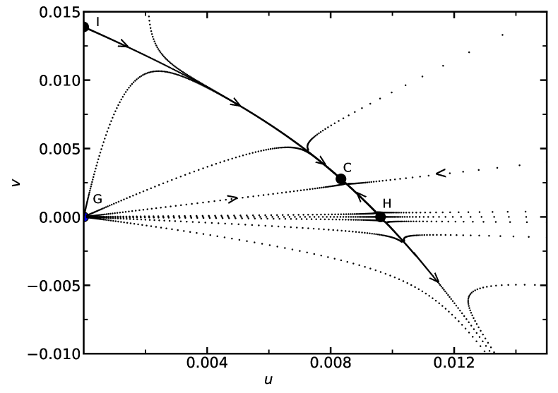
Figure 1: We have numerically integrated the one-loop flow equations (2) for $N=5$ and $\epsilon=1$. The fixed points are given as solid circles. The fixed points are labeled as G (Gaussian), I (decoupled Ising), H ($O(N)$-invariant Heisenberg), and C (cubic). Selected RG trajectories are given by dotted lines. Subsequent dots are separated by a scale factor of $b=2^{1/8}$. Hence, the larger the distance between the dots, the faster the flow. The arrows indicate the direction of the flow.

In the present work, we provide accurate estimates of critical exponents for the cubic fixed point for $N=3$ and $4$. To this end, we study a lattice version of the Hamiltonian (1) with two parameters. We generalize the idea of an improved model to a two-parameter model. The idea to study improved models to get better precision on universal quantities goes back to Refs. ChFiNi ; FiCh . First studies of improved models using finite-size scaling (FSS) Barber and Monte Carlo simulations applied to the three-dimensional Ising universality class are Refs. Bloete ; Ballesteros ; KlausStefano ; myPhi4 . For a discussion see, for example, Sec. 2.3 of the review PeVi02 . For the application to the three-dimensional Heisenberg universality class, see Refs. O34 ; ourHeisen ; O234 ; myIco . By using finite-size scaling, one tunes the parameter of the reduced Hamiltonian such that the amplitude of the leading correction vanishes. Here in the case of the cubic fixed point, we are tuning two parameters to eliminate the amplitudes of the two leading corrections. Since one of the correction exponents is much smaller than one, improving the reduced Hamiltonian turns out to be absolutely crucial to get reliable results for the critical exponents of the cubic fixed point.

In our simulations we consider $N=4$ in addition to $3$. It is not of direct experimental relevance. However, here we expect that the cubic fixed point is well separated from the $O(4)$-invariant one, and therefore the conceptual points of our study can be more easily demonstrated in this case. Furthermore, our results allow to benchmark field-theoretic methods that produce estimates for any value of $N$.

The outline of the paper is the following: In the next section we define the model and the observables that we measure. In Sec. III we discuss the Monte Carlo algorithms that are used for the simulation. In Sec. IV we summarize the theoretical predictions for the FSS behavior of dimensionless quantities. In Sec. V we discuss the simulations and the analysis of the data for $N=4$. For $N=3$ we first perform high statistics simulations at the $O(3)$-invariant point to improve the accuracy of the estimate of the exponent $Y_{4}$ (see Sec. VI). Next, in Sec. VI, we discuss simulations for a finite perturbation with cubic symmetry. We locate the improved model by analyzing the FSS behavior of dimensionless quantities. Estimates of the critical exponents $\eta$ and $\nu$ are obtained by analyzing the FSS behavior of the magnetic susceptibility and the slope of dimensionless quantities at criticality. Finally, we summarize our results and compare them with estimates given in the literature.

II The model and observables

In our study we consider a discretized version of the continuum Hamiltonian (1) on a simple cubic lattice. We extend the reduced Hamiltonian of the $\phi^{4}$ model [see, for example, Eq. (1) of Ref. ourHeisen ] by a term proportional to

$$\sum_{a}Q_{4,aaaa}(\vec{\phi}\,)=\sum_{a}\phi_{x,a}^{4}-\frac{3}{N+2}\left(\vec{\phi}_{x}^{\,2}\right)^{2}\;,$$ (3)

with cubic symmetry, breaking $O(N)$ invariance

$${\cal H}(\{\vec{\phi}\,\})=-\beta\sum_{<xy>}\vec{\phi}_{x}\cdot\vec{\phi}_{y}+\sum_{x}\left[\vec{\phi}_{x}^{\,2}+\lambda(\vec{\phi}_{x}^{\,2}-1)^{2}+\mu\left(\sum_{a}\phi_{x,a}^{\,4}-\frac{3}{N+2}\left(\vec{\phi}_{x}^{\,2}\right)^{2}\right)\right]\;,$$ (4)

where $\vec{\phi}_{x}$ is a vector with $N$ real components. The subscript $a$ denotes the components of the field and $\{\vec{\phi}\,\}$ is the collection of the fields at all sites $x$. We label the sites of the simple cubic lattice by $x=(x_{0},x_{1},x_{2})$, where $x_{i}\in\{1,2,\ldots,L_{i}\}$. Furthermore, $<xy>$ denotes a pair of nearest neighbors on the lattice. In our study, the linear lattice size $L=L_{0}=L_{1}=L_{2}$ is equal in all three directions throughout. We employ periodic boundary conditions. The real numbers $\beta$, $\lambda$ and $\mu$ are the parameters of the model. Note that $Q_{4}$ is the traceless symmetric combination of four instances of the field [see, for example, Eq. (7) of Ref. O234 ]

$$Q_{4,abcd}(\vec{\Phi}\,) = \Phi_{a}\Phi_{b}\Phi_{c}\Phi_{d}$$ (5)

$$- {1\over N+4}\vec{\Phi}^{\,2}\left(\delta_{ab}\Phi_{c}\Phi_{d}+\delta_{ac}\Phi_{b}\Phi_{d}+\delta_{ad}\Phi_{b}\Phi_{c}+\delta_{bc}\Phi_{a}\Phi_{d}+\delta_{bd}\Phi_{a}\Phi_{c}+\delta_{cd}\Phi_{a}\Phi_{b}\right)$$

$$+ {1\over(N+2)(N+4)}(\vec{\Phi}^{\,2})^{2}\left(\delta_{ab}\delta_{cd}+\delta_{ac}\delta_{bd}+\delta_{ad}\delta_{bc}\right)\;.$$

The expectation value of $\sum_{a}Q_{4,aaaa}(\vec{\phi}\,)$ vanishes for an $O(N)$-symmetric distribution of $\vec{\phi}$. A small perturbation of the $O(N)$-symmetric system, $\mu=0$, only affects scaling fields with the symmetries corresponding to the cubic symmetry of the perturbation. See also Eq. (5) of Ref. CB_O3 and the accompanying discussion.

Note that in the Hamiltonian (4) the components of the field decouple for $\lambda-\frac{3}{N+2}\mu=0$. Since the term $\sum_{x}\vec{\phi}_{x}^{\,2}$ has the factor $(1-2\lambda)$ and $\sum_{x}\sum_{a}\phi_{x,a}^{4}$ the factor $\mu=\frac{N+2}{3}\lambda$ in front, a rescaling of the field $\phi_{x}$ is needed to match with the Hamiltonian

$${\cal H}(\{\phi\})=-\tilde{\beta}\sum_{<xy>}\phi_{x}\phi_{y}+\sum_{x}\left[\phi_{x}^{2}+\tilde{\lambda}(\phi_{x}^{2}-1)^{2}\right]\;,$$ (6)

considered for example in ref. myPhi4 , where $\phi_{x}$ is a real number. We arrive at the equations

$$(1-2\lambda)=(1-2\tilde{\lambda})\;c\;\;,\;\;\;\;\frac{N+2}{3}\lambda=\tilde{\lambda}\;c^{2}$$ (7)

and hence

$$\frac{6}{N+2}\tilde{\lambda}\;c^{2}+(1-2\tilde{\lambda})\;c-1=0$$ (8)

with the solutions

$$c=\frac{-(1-2\tilde{\lambda})\pm\sqrt{(1-2\tilde{\lambda})^{2}+\frac{24}{N+2}\tilde{\lambda}}}{\frac{12}{N+2}\tilde{\lambda}}\;\;,$$ (9)

where we take the positive solution. Plugging in $\tilde{\lambda}^{*}\approx 1.1$ myPhi4 we arrive at $c=1.43647586...$ for $N=3$. Note that $\tilde{\lambda}^{*}$ denotes the value of $\tilde{\lambda}$, where leading corrections to scaling vanish. Hence we get for the improved decoupled model $\lambda^{*}=1.361885...$, $\mu^{*}=\frac{N+2}{3}\lambda^{*}=2.269809...$, and $\tilde{\beta}_{c}=0.3750966(4)$ at $\tilde{\lambda}=1.1$ translates to $\beta_{c}=c\tilde{\beta}_{c}=0.5388172...\;$. For $N=4$ we get $\lambda^{*}=1.486347...$, $\mu^{*}=2.972695...$, and $\beta_{c}=0.616626...\;$.

II.1 The observables and dimensionless quantities

Dimensionless quantities or phenomenological couplings play a central role in finite size scaling. Similar to the study of $O(N)$-invariant models we study the Binder cumulant $U_{4}$, the ratio of partition functions $Z_{a}/Z_{p}$ and the second moment correlation length over the linear lattice size $\xi_{2nd}/L$. Let us briefly recall the definitions of the observables and dimensionless quantities that we measure.

The energy of a given field configuration is defined as

$$E=\sum_{<xy>}\vec{\phi}_{x}\cdot\vec{\phi}_{y}\;\;.$$ (10)

The magnetic susceptibility $\chi$ and the second moment correlation length $\xi_{2nd}$ are defined as

$$\chi\equiv\frac{1}{V}\left\langle\Big{(}\sum_{x}\vec{\phi}_{x}\Big{)}^{2}\right\rangle\;\;,$$ (11)

where $V=L^{3}$ and

$$\xi_{2nd}\equiv\sqrt{\frac{\chi/F-1}{4\sin^{2}\pi/L}}\;\;,$$ (12)

where

$$F\equiv\frac{1}{V}\left\langle\Big{|}\sum_{x}\exp\left(i\frac{2\pi x_{k}}{L}\right)\vec{\phi}_{x}\Big{|}^{2}\right\rangle$$ (13)

is the Fourier transform of the correlation function at the lowest non-zero momentum. In our simulations, we have measured $F$ for the three directions $k=0,1,2$ and have averaged these three results.

The Binder cumulant $U_{4}$ is given by

$$U_{4}\equiv\frac{\langle(\vec{m}^{2})^{2}\rangle}{\langle\vec{m}^{2}\rangle^{2}},$$ (14)

where $\vec{m}=\frac{1}{V}\,\sum_{x}\vec{\phi}_{x}$ is the magnetization of a given field configuration. We also consider the ratio $Z_{a}/Z_{p}$ of the partition function $Z_{a}$ of a system with anti-periodic boundary conditions in one of the three directions and the partition function $Z_{p}$ of a system with periodic boundary conditions in all directions. This quantity is computed by using the cluster algorithm. For a discussion see Appendix A 2 of ref. XY1 .

In order to detect the effect of the cubic anisotropy we study

$$U_{C}=\frac{\langle\sum_{a}Q_{4,aaaa}(\vec{m})\rangle}{\langle\vec{m}^{\,2}\rangle^{2}}\;.$$ (15)

In the following we shall refer to the RG-invariant quantities $U_{C}$, $U_{4}$, $Z_{a}/Z_{p}$, and $\xi_{2nd}/L$ by using the symbol $R$.

In our analysis we need the observables as a function of $\beta$ in some neighborhood of the simulation point $\beta_{s}$. To this end we have computed the coefficients of the Taylor expansion of the observables up to the third order. For example the first derivative of the expectation value $\langle A\rangle$ of an observable $A$ is given by

$$\frac{\partial\langle A\rangle}{\partial\beta}=\langle AE\rangle-\langle A\rangle\langle E\rangle\;\;.$$ (16)

In the case of decoupled systems, $\lambda-\frac{N+2}{3}\mu=0$, we can express the dimensionless quantities introduced above in terms of their Ising counterparts. For example

$$U_{C}=\frac{N-1}{N(N+2)}(U_{4,Ising}-3)\;\;.$$ (17)

Hence, we get for the fixed point value, which is indicated by ^∗

$$U_{C,DI}^{*}=(1.60359(4)-3)\frac{N-1}{N(N+2)}=-1.39641(4)\frac{N-1}{N(N+2)}$$ (18)

using the result of myIso for $U_{4,Ising}^{*}$. Furthermore, $(Z_{a}/Z_{p})^{*}_{DI}=((Z_{a}/Z_{p})^{*}_{Ising})^{N}$, $U_{4,DI}^{*}=\frac{1}{N}U_{4,Ising}^{*}+\frac{N-1}{N}$, and $(\xi_{2nd}/L)^{*}_{DI}=(\xi_{2nd}/L)^{*}_{Ising}$, where the subscript $DI$ indicates the decoupled Ising fixed point.

III Monte Carlo algorithm

In previous work (see, for example, Refs. O34 ; O234 ; myON ) we have simulated the $O(N)$-invariant $\phi^{4}$ model on the simple cubic lattice. Here, for $N=4$, we use the algorithm and C-code of ref. myON with minor modifications, to take into account the term proportional to $\mu$ in the reduced Hamiltonian (4). For $N=3$, we have implemented the algorithm by using AVX intrinsics to speed up the simulation.

The algorithm used in ref. myON is a hybrid of:

• wall cluster algorithm KlausStefano ;

• local Metropolis update;

• local over-relaxation update;

• global rotation of the field.

In the case of the wall cluster update, in ref. myON , we performed the update for technical reasons componentwise. This means that in a given update step only the sign of a single component of the field might change. This way, the value of $\sum_{a}Q_{4,aaaa}(\vec{\phi}_{x})$ remains unchanged. Hence, we can take this part of the C-program from Ref. myON without any change. Also the measurement of $Z_{a}/Z_{p}$, which is integrated into the wall cluster update, is reused without change.

In the local Metropolis algorithm, we generate a proposal by

$$\phi_{x,i}^{\prime}=\phi_{x,i}+s(r_{i}-0.5)$$ (19)

for each component $i$ of the field at the site $x$. $r_{i}$ is a uniformly distributed random number in $[0,1)$ and the step size $s$ is tuned such that the acceptance rate is roughly $50\%$. Note that for each component a random number $r_{i}$ is taken. We use the acceptance probability

$$P_{acc}=\mbox{min}\left[1,\exp(-H(\{\vec{\phi}\,\}^{\prime})+H(\{\vec{\phi}\,\})\right]\;.$$ (20)

The only change compared with the program of Ref. myON is that we have to take into account the term $\mu\sum_{a}Q_{4,aaaa}(\vec{\phi}_{x})$, when computing $\Delta H(\{\vec{\phi}\,\}^{\prime},\{\vec{\phi}\,\})=H(\{\vec{\phi}\,\}^{\prime})-H(\{\vec{\phi}\,\})$.

We have implemented over-relaxation updates

$$\vec{\phi}_{x}^{\;\;{}^{\prime}}=2\frac{\vec{\Phi}_{x}\cdot\vec{\phi}_{x}}{\vec{\Phi}_{x}^{2}}\vec{\Phi}_{x}-\vec{\phi}_{x}\;\;,$$ (21)

where

$$\vec{\Phi}_{x}=\sum_{y.nn.x}\vec{\phi}_{y}\;\;,$$ (22)

where $\sum_{y.nn.x}$ is the sum over all nearest neighbors $y$ of the site $x$. In the case of the $O(N)$-invariant $\phi^{4}$ model this update does not change the value of the Hamiltonian and therefore no accept/reject step is needed. Here, the value of the term $\mu\sum_{a}Q_{4,aaaa}(\vec{\phi}_{x})$ changes under the update, which has to be taken into account in an accept/reject step (20). This update has no parameter which can be tuned. The acceptance rate depends on the parameters of the model. In particular, the larger $\mu$, the smaller the acceptance rate. It turns out that for the range of $\mu$ studied here the acceptance rate is reasonably high. For example, for $N=4$, for $(\lambda,\mu)=(7,2.64)$, which is close to the improved point $(\lambda,\mu)^{*}$, we get an acceptance rate of about $0.77$ at the critical point, with little dependence on the lattice size. In the case of $N=3$, the values of $\mu$ that we simulated at are smaller and hence the acceptance rates are even larger.

In Ref. myON we use global rotations of the field to compensate for the fact that the cluster update has preferred directions. The global rotation changes the value of the new term $\sum_{x}\mu\sum_{a}Q_{4,aaaa}(\vec{\phi})$. Hence, an accept/reject step has to be introduced. In addition, we introduced a step size for the global rotation, which is tuned such that the acceptance rate is very roughly $1/2$. For simplicity we did not perform a general $O(N)$ rotation, but used a rotation among two of the components. It turned out that these global rotations are useful only for small $\mu$ and/or small linear lattice sizes $L$. In particular for $\mu$ of the order of $\mu^{*}$, the reduction in the autocorrelation times, for reasonable lattice sizes, does not pay off for the computational costs of the rotation. Therefore, eventually, we skipped this component of the update. Unfortunately this leaves us with the potential problem that the cluster update discussed above only changes the sign of a given component of the field.

In fact, for lattice sizes $L\gtrapprox 32$ it turned out to be advantageous to add cluster updates that exchange two components of the field

$$\phi_{x,j}^{\prime}=\phi_{x,i}\;\;,\;\phi_{x,i}^{\prime}=\phi_{x,j}$$ (23)

for $i\neq j$, while the other components stay unchanged. Note that this update leaves the term $\sum_{a}Q_{4,aaaa}(\vec{\phi}_{x})$ unchanged. The update can be written as a reflection

$$\vec{\phi}_{x}^{\prime}=\vec{\phi}_{x}-2(\vec{r}\cdot\vec{\phi}_{x})\vec{r}$$ (24)

with $r_{i}=2^{-1/2}$, $r_{j}=-2^{-1/2}$, and $r_{k}=0$ for $k\neq i,j$. The cluster update can also be performed with an additional change of the sign:

$$\phi_{x,j}^{\prime}=-\phi_{x,i}\;\;,\;\phi_{x,i}^{\prime}=-\phi_{x,j}$$ (25)

for $i\neq j$, while the other components stay unchanged. For simplicity, we have implemented this update as single-cluster update Wolff . With probability $1/2$ we took either eq. (23) or eq. (25) for a given cluster update.

During the major part of the simulations, we did not measure autocorrelation times, since we performed binning of the data at run time. In preliminary simulations, where we performed of the order of $10^{6}$ update cycles, we stored all measurement. In the analysis we computed integrated autocorrelation times for a selection of observables that we studied.

In the case of $N=4$ an update and measurement cycle is given by the following C-code:
over(); rotate(); metro(); for(ic=0;ic<N;ic++) wall_0(ic); measure();
over(); rotate(); metro(); for(ic=0;ic<N;ic++) wall_1(ic); measure();
over(); rotate(); metro(); for(ic=0;ic<N;ic++) wall_2(ic); measure();
Here over() is a sweep with the over-relaxation update over the lattice. rotate() is the global rotation of the field. For larger lattices, we have skipped the rotation. metro() is a sweep with the Metropolis update discussed above, followed by an over-relaxation update at the same site. wall_k(ic) is a wall-cluster update with a plane perpendicular to the k-axis. The component ic of the field is updated. measure() contains the evaluation of the observables discussed above.

In the most recent version of the program, a sequence of single-cluster updates replaces rotate(). The sequence is given by
for(j=0;j<L/8;j++) for(l=0;l<N-1;l++) for(k=l+1;l<N;l++) single(l,k);
where single(l,k) is a single-cluster update, exchanging the components l and k for the sites within the cluster.

In Table 1 we give integrated autocorrelation times for the energy, the magnetic susceptibility $\chi$, and $Q_{4}(\vec{m})$ for $(\lambda,\mu)=(7,2.64)$, which is close to $(\lambda,\mu)^{*}$, at $\beta=0.86407506$, which is our estimate of $\beta_{c}$. We truncated the summation of the integrated autocorrelation function at $t_{max}=6\tau_{int,E}$ for all quantities considered. Throughout we performed $10^{6}$ measurements. Note that adding the single-cluster updates increases the CPU time needed for one update cycle by about 40 $\%$. Hence already for $L=32$ we see an advantage for adding the single-cluster updates.

Table 1: Estimates of the integrated autocorrelation time $\tau_{int}$ of the energy $E$, the magnetic susceptibility $\chi$, and $Q_{4}(\vec{m})$ for $N=4$, at $(\lambda,\mu)=(7,2.64)$ and $\beta=0.86407506$. ”single” and ”no single” refer to simulations that have component exchanging single-cluster updates or not. For a discussion see the text.

$L$	type	$t_{max}$	$\tau_{int,E}$	$\tau_{int,\chi}$	$\tau_{int,Q_{4}}$
16	no single	30	4.76(5)	3.58(3)	2.37(3)
16	single	21	3.38(3)	2.30(2)	1.57(1)
32	no single	38	6.16(7)	4.48(5)	3.34(4)
32	single	26	4.20(4)	2.40(2)	1.63(2)
64	no single	50	8.29(11)	5.65(7)	4.62(7)
64	single	31	5.09(5)	2.44(2)	1.50(2)
128	no single	68	11.13(17)	7.24(11)	6.11(12)
128	single	38	6.35(7)	2.51(3)	1.41(2)

In the case of $N=3$, we implemented the algorithm by using the AVX instruction set of x86 CPUs. These were accessed by using AVX intrinsics. AVX instructions act on several variables that are packed into 256 bit units in parallel. In particular we used __m256d variables to store 4 double precision floating point numbers. We employed a trivial parallelization, simulating four systems in parallel. Each of the floating point numbers in a __m256d variable is associated with one of the four systems that is simulated. This way, we could speed up the local updates and the measurement of the observables by a factor somewhat larger than two. To this end we reused the random number $r^{(0)}$ that is uniformly distributed in $[0,1)$ by

$$r^{(j)}=\mbox{frac}(r^{(0)}+j/4)\;,$$ (26)

where $j=0$, $1$, $2$, or $3$ and frac is the fractional part of a real number. A discussion on the reuse of random numbers is given in Appendix A of Ref. ourDynamic .

In the case of the cluster algorithm we found no efficient use of the parallel execution using AVX instruction. Therefore, we go through the four copies of the field sequentially. Here, the data layout is a small obstacle. Therefore, the overall gain obtained by using the parallelization as discussed above is at the level of about $20\%$.

Since the overall gain is rather modest compared with a plain C implementation, we abstain from a detailed discussion of the implementation. We experimented with the composition of the update cycle. It turns out that the dependence of the efficiency on the precise composition is rather flat. Similar to $N=4$, it is clearly advantageous to add cluster updates that exchange components of the field. The update and measurement cycles used in most of our simulations are similar to those discussed above for $N=4$. Motivated by the speedup of the local updates by the AVX implementation, however, the relative number of local over-relaxation updates compared with the cluster updates is increased.

IV Finite-size scaling

In this section we recall the theoretical basis of the FSS analysis of dimensionless quantities. In particular, we consider the ratio of partition functions $Z_{a}/Z_{p}$, the second moment correlation length over the linear lattice size $\xi_{2nd}/L$, the Binder cumulant $U_{4}$, and the quantity $U_{C}$ that quantifies the violation of the $O(N)$ symmetry. First we consider the neighborhood of a single fixed point, being well separated from other fixed points. In previous work, we discussed the case of a single correction with a correction exponent $\omega$ being clearly smaller than two. Here we discuss the case of two such corrections with the exponents $\omega_{2}<\omega_{1}<2$, which is the case for the cubic fixed point.

This turns out to be sufficient for the analysis of the cubic fixed point for $N=4$. However, for $N=3$ it is desirable to extend the discussion to the neighborhood of two fixed points that are close to each other.

IV.1 Dimensionless quantities in the neighborhood of a fixed point

Dimensionless quantities $R_{i}$, for a given geometry, are functions of the lattice size $L$ and the parameters $\beta$, $\lambda$, and $\mu$ of the reduced Hamiltonian. Throughout, we consider a vanishing external field $h=0$. In the neighborhood of a critical point, we might also write them as a function of the nonlinear scaling fields $u_{j}$ and the linear lattice size $L$:

$$R_{i}(\beta,\lambda,\mu,L)=R_{i}(u_{t}L^{y_{t}},u_{3}L^{y_{3}},u_{4}L^{y_{4}},\{u_{j}L^{y_{j}}\})\;,$$ (27)

where we identify $y_{3}=-\omega_{2}$ and $y_{4}=-\omega_{1}$ in the case of the cubic fixed point. $y_{t}=1/\nu$ is the thermal RG exponent. Note that $y_{3}>y_{4}>-1$, while we expect, similar as for the $O(N)$-invariant models, $y_{j}\lessapprox-2$ for $j>4$. The non-linear scaling fields can be written as (see, for example, Ref. PeVi02 , sec. 1.5.7)

$$u_{t}=t+g_{11}(\lambda,\mu)t^{2}+O(t^{3})\;,$$ (28)

where $t=\beta-\beta_{c}$ is the reduced temperature, and $\beta_{c}$ is the inverse critical temperature. For simplicity, in the definition of $t$, we have skipped the normalization $1/\beta_{c}$ and took the opposite sign as usual. The irrelevant scaling fields are

$$u_{3}=g_{13}(\lambda,\mu)+g_{23}(\lambda,\mu)t+O(t^{2})$$ (29)

and

$$u_{4}=g_{14}(\lambda,\mu)+g_{24}(\lambda,\mu)t+O(t^{2})\;.$$ (30)

Now let us expand $R_{i}$ on the right-hand side of eq. (27) around the fixed point $u_{j}L^{y_{j}}=0$:

$$R_{i}(\beta,\lambda,\mu,L)=R_{i}^{*}+\sum_{j}r_{i,j}u_{j}L^{y_{j}}+\frac{1}{2}\sum_{j,k}r_{i,j,k}u_{j}u_{k}L^{y_{j}+y_{k}}+...\;,$$ (31)

where $j=t,3,4,...$ and

$$r_{i,j}=\frac{\partial R_{i}}{\partial(u_{j}L^{y_{j}})}$$ (32)

and

$$r_{i,j,k}=\frac{\partial^{2}R_{i}}{\partial(u_{j}L^{y_{j}})\partial(u_{k}L^{y_{k}})}$$ (33)

at the fixed point. Now putting in the expressions for the scaling fields $u_{j}$ we arrive at

$$R_{i}(\beta_{c},\lambda,\mu,L)=R_{i}^{*}+\sum_{j\geq 3}r_{i,j}g_{1j}(\lambda,\mu)L^{y_{j}}+...\;$$ (34)

at the critical temperature. Eq. (34) is the basis for the Ansätze used to fit our data. Note that we have simulated at $\beta_{s}\approx\beta_{c}$. In addition to the value of $R_{i}(\beta_{s},\lambda,\mu,L)$, we determine the Taylor coefficients of the expansion of $R_{i}$ in $(\beta-\beta_{s})$ up to the third order. In our fits, we keep $R_{i}(\beta_{s},\lambda,\mu,L)$ on the left side of the equation, and bring the terms proportional to $(\beta_{c}-\beta_{s})^{\alpha}$ for $\alpha=1$, $2$, and $3$ to the left. Furthermore, we ignore the statistical error of the Taylor coefficients. This way, we can treat $\beta_{c}$ as a free parameter in the fit.

In order to arrive at an Ansatz that can be used in a fit, we have to truncate eq. (34). After a few numerical experiments we took

$$R_{i}(\beta_{c},\lambda,\mu,L) = R_{i}^{*}+r_{i,3}u_{3}(\lambda,\mu)L^{y_{3}}+\frac{1}{2}q_{i,3}(r_{i,3}u_{3}(\lambda,\mu)L^{y_{3}})^{2}$$ (35)

$$+ r_{i,4}u_{4}(\lambda,\mu)L^{y_{4}}+q(\beta_{c},\lambda,\mu,L)\;$$

as our standard Ansatz. To simplify the notation, we identify $u_{j}=g_{1,j}$ here. We set $r_{4,3}=1$ and $r_{3,4}=1$, where $i=3$ corresponds to the Binder cumulant $U_{4}$ and $i=4$ to $U_{C}$. We have skipped terms that mix $u_{3}$ and $u_{4}$, since we simulated at parameters $(\lambda,\mu)$, where at least one of the scaling fields has a small amplitude. Below, analyzing the data, we specify how we parametrize $u_{3}$ and $u_{4}$. $q(\beta_{c},\lambda,\mu,L)$ contains the corrections that decay with $L^{-\epsilon}$, where $\epsilon\gtrapprox 2$. For $Z_{a}/Z_{p}$, we assumed that there are only corrections due to the breaking of the symmetry by the cubic lattice. We assume that the amplitude of this correction does not depend on $\mu$ and $\lambda$. As in our previous work, we take $\epsilon_{2}=2.023$ as numerical value of the exponent. In the case of the other three quantities there are corrections with the exponent $\epsilon_{1}=2-\eta$ due to the analytic background of the magnetic susceptibility. We write the coefficient of these corrections as linear functions of $\lambda$ and $\mu$. In the case of the Binder cumulant $U_{4}$ and the new cumulant, we do not take into account the correction due to the breaking of the symmetry by the lattice. We expect that it is at least partially taken into account by the term with the exponent $\epsilon_{1}$. For $\xi_{2nd}/L$, we expect that there is even a third correction, and that there are huge cancellations between the terms. Therefore we have added in this case a second correction. We took a constant amplitude and the exponent $\epsilon_{2}=2.023$. Obviously, this Ansatz suffers from truncation errors. The effect of these errors can be checked by varying the range of $\lambda$ and $\mu$ and the linear lattice sizes $L$ that are taken into account.

IV.2 Two fixed points in close neighborhood

Generically for a perturbation of a conformally invariant fixed point (see, for example, frad ) one gets

$$\frac{\mbox{d}g_{i}}{\mbox{d}l}=y_{i}g_{i}-C_{kli}g_{k}g_{l}+...\;,$$ (36)

where $y_{i}$ is the RG exponent of the perturbation, $C_{kli}$ is a structure constant, up to a constant factor, set by convention, and $g_{i}$ a dimensionless coupling. Here we consider a single relevant perturbation with $0<y\ll 1$. We get

$$\frac{\mbox{d}g}{\mbox{d}l}=yg-Cg^{2}+O(g^{3})\;.$$ (37)

Note that the authors of Ref. AharonyNeu discuss the same equation [their Eq. (11)], where $y$ and $C$ are obtained from the analysis of the six-loop $\epsilon$ expansion. See also Eq. (27) of Ref. CB_O3 . Here $y$ and $C$ are free parameters that are eventually fixed by fitting numerical data. We assume $g$ to be small and hence ignore the $O(g^{3})$ contributions in the following. In addition to the fixed point $g=0$, there is the fixed point

$$g^{*}=\frac{y}{C}\;.$$ (38)

Let us rewrite Eq. (37) by using $\delta=g-g^{*}$:

$$\frac{\mbox{d}\delta}{\mbox{d}l}=y(g^{*}+\delta)-C(g^{*}+\delta)^{2}=-y\delta-C\delta^{2}\;.$$ (39)

Hence at the fixed point $g=g^{*}$, there is an irrelevant perturbation with RG exponent $-y$.

With respect to our finite size scaling study, we vary the linear lattice size $L$, while the coupling at the cutoff scale is given. The differential equation $g^{\prime}=yg-Cg^{2}$ is discussed in various contexts in the literature and one finds the solution

$$g=\frac{y}{C+p\exp(-yl)}\;,$$ (40)

where $p$ is an integration constant. Solving for $p$, for given $g_{0}$ at the scale $\exp(l_{0})$, we get

$$g=\frac{g^{*}}{1+\left(\frac{g^{*}}{g_{0}}-1\right)\exp(-y[l-l_{0}])}\;.$$ (41)

The coupling constant $g_{0}$ should be an analytic function of the parameters of the model

$$g_{0}=r(\lambda)\mu+s(\lambda)\mu^{2}+...\;.$$ (42)

The dimensionless quantity $U_{C}$ at the critical point is an analytic function of $g$ at the scale proportional to $L=\exp(l)$, where $L$ is the linear size of the lattice

$$U_{C}(g)=Ag+Bg^{2}+...\;.$$ (43)

Taking the leading order in Eqs. (42) and (43) only, we arrive at

$$U_{C}(\mu,\lambda,L)=\frac{U_{C}^{*}}{1+q\left(\frac{\mu^{*}}{\mu}-1\right)L^{-y}}\;,$$ (44)

where $U_{C}^{*}=Ag^{*}$ and $r\mu^{*}=g^{*}$. The factor $q$ reflects the uncertainty of the identification of the length scales. $\mu^{*}$ and $q$ might depend on $\lambda$.

V The simulations and the analysis for $N=4$

First we have simulated the model for $N=4$. Here the $O(N)$ invariant and the cubic fixed point are better separated than for $N=3$, which should make the analysis of the data more simple. First we performed simulations for $\lambda=18.5$ at various values of $\mu$. Note that for the $O(4)$-invariant $\phi^{4}$ model $\lambda^{*}=18.4(9)$ myON . Extensive simulations for $\mu=0$, were performed for $\lambda=18.5$ in Ref. myON . In the preliminary stage of the analysis we mainly monitored $\bar{U}_{C}$, which is $U_{C}$ at the value of $\beta$ such that $[Z_{a}/Z_{p}](\beta)=0.11911$. Note that $(Z_{a}/Z_{p})^{*}=0.11911(2)$ for the $O(4)$-invariant $\phi^{4}$ model on a $L^{3}$ torus myON .

The cubic fixed point is identified by $\bar{U}_{C}$ not depending on the linear lattice size $L$. We arrived at $\bar{U}_{C}^{*}\approx-0.086$ and $\mu^{*}\approx 3.5$. However, a more detailed analysis of the data showed that for $(\lambda,\mu)=(18.5,3.5)$, corrections $\propto L^{-\omega_{1}}$ with $\omega_{1}\approx 0.8$ have a considerable magnitude. Prompted by this result we started a more general search for $(\lambda,\mu)^{*}$, where both leading and subleading corrections are vanishing. As preliminary estimate we arrived at $(\lambda,\mu)^{*}\approx(7,2.7)$.

In particular, to get accurate estimates of the correction exponents, we simulated at various values of $(\lambda,\mu)$, focussing on the neighborhood of $(\lambda,\mu)^{*}$. The data sets used in our final analysis, containing 20 different pairs $(\lambda,\mu)$, are summarized in Table 2.

For most of these pairs we simulated the linear lattice sizes $L=12$, $14$, $16$, $18$, $20$, $24$, $28$, $32$, $40$, $48$, and $56$. More, and in particular larger lattice sizes were added for $(\lambda,\mu)=(18.5,3.5)$, $(18.5,4)$, $(7,2.64)$, and $(7,3)$ in order to determine the critical exponents $\nu$ and $\eta$. In particular for $(\lambda,\mu)=(7,2.64)$, which is close to our final estimate of $(\lambda,\mu)^{*}$, we have simulated in addition $L=6$, $7$, $8$, $9$, $10$, $11$, $13$, $15$, $64$, $72$, $80$, and $100$. For example, for $(\lambda,\mu)=(7,2.64)$, we performed between $10^{9}$ and $3\times 10^{9}$ measurements for $L=6$ up to $32$. Then the statistics is going down with increasing lattice size. For $L=100$, we performed $1.3\times 10^{8}$ measurements. In total we have used the equivalent of about $22$ years of CPU time on a single core of an AMD EPYC^TM 7351P CPU.

V.1 Dimensionless quantities

First we have analyzed the dimensionless quantities by using a joint fit of all four quantities that we have measured and all 20 pairs of $(\lambda,\mu)$. To this end, we used the Ansatz (35). We used $u_{3}(\lambda,\mu)$ and $u_{4}(\lambda,\mu)$ as free parameters for each pair $(\lambda,\mu)$.

Already for $L_{min}=12$ we find an acceptable $\chi^{2}/$DOF$=0.999$ corresponding to a $p$-value $p=0.504$. In table 2 we give the correction amplitudes $u_{3}$ and $u_{4}$ for each $(\lambda,\mu)$, and the estimate of $\beta_{c}$. In the case of $u_{3}$ and $u_{4}$ we give the statistical error for this particular fit only. In Fig. 2 we plot the estimates of $u_{3}$ and $u_{4}$. Note that we avoided values of $(\lambda,\mu)$, where both $u_{3}$ and $u_{4}$ have a large modulus. This way we tried to reduce the effect of corrections that contain both scaling fields $u_{3}$ and $u_{4}$.

In order to get the final estimate of $\beta_{c}$, the dimensionless quantities $R_{i}$ and the correction exponents $\omega_{1}$ and $\omega_{2}$ and their error, we produced a set of estimates with their respective statistical error. To this end, we take Ansatz (35) for $L_{min}=12$ and $16$. Furthermore, we extended Ansatz (35) in four different ways or skipped one pair of $(\lambda,\mu)$:

• adding a term proportional to $L^{-4}$;

• adding a term proportional $u_{3}L^{-\omega_{2}}$ to the third power;

• adding a term proportional $u_{4}L^{-\omega_{1}}$ to the second power;

• adding a mixed $u_{3}u_{4}L^{-\omega_{2}-\omega_{1}}$ term;

• skipping $(\lambda,\mu)=(2,1.16)$ from the data.

These are all taken at $L_{min}=12$, giving all $\chi^{2}/$DOF $\approx 1$. We compute the minimum $\beta_{c,min}$ of $\beta_{c}-error$ for each pair $(\lambda,\mu)$ among these different estimates. The same is done for the maximum $\beta_{c,max}$ of $\beta_{c}+error$. As our final estimate we take $(\beta_{c,max}+\beta_{c,min})/2$ and $(\beta_{c,max}-\beta_{c,min})/2$ as error. The results are given in the last column of Table 2.

Table 2: Amplitudes $u_{3}$ and $u_{4}$ of the corrections obtained by fitting our data for dimensionless quantities for $N=4$ for $L_{min}=12$ by using the Ansatz (35). In the last column, we give the estimate of $\beta_{c}$. Details are discussed in the text.

$\lambda$	$\mu$	$u_{3}$	$u_{4}$	$\beta_{c}$
2	1.16	–0.00006(12)	0.03235(79)	0.77776644(85)
4	1.9	0.00060(10)	0.01192(32)	0.83415315(38)
6	2.5	–0.00134(10)	0.00244(9)	0.85567074(29)
6	2.93	–0.00996(16)	–0.00035(15)	0.84735549(45)
6.5	2.4	0.00311(11)	0.00223(11)	0.86309955(34)
6.5	2.7	–0.00324(10)	0.00037(8)	0.85790473(32)
7	2.2	0.00974(17)	0.00251(18)	0.87097872(53)
7	2.5	0.00287(10)	0.00087(9)	0.86635289(24)
7	2.64	–0.00004(10)	0.00008(7)	0.86407506(17)
7	2.7	–0.00126(10)	–0.00030(8)	0.86307673(28)
7	3	–0.00688(12)	–0.00205(15)	0.85789401(27)
7.2	2.656	0.00035(10)	–0.00028(8)	0.86566530(27)
7.5	2.6	0.00251(10)	–0.00034(8)	0.86913520(28)
7.5	2.8	–0.00143(10)	–0.00146(9)	0.86598689(39)
7.5	3	–0.00509(11)	–0.00262(14)	0.86270900(33)
8	2.43	0.00767(14)	–0.00008(11)	0.87542511(43)
8	2.5	0.00615(12)	–0.00041(10)	0.87443835(37)
8	2.9	–0.00173(10)	–0.00252(11)	0.86849718(33)
18.5	3.5	0.00312(11)	–0.00994(26)	0.89931064(30)
18.5	4	–0.00352(10)	–0.01173(37)	0.89496905(38)

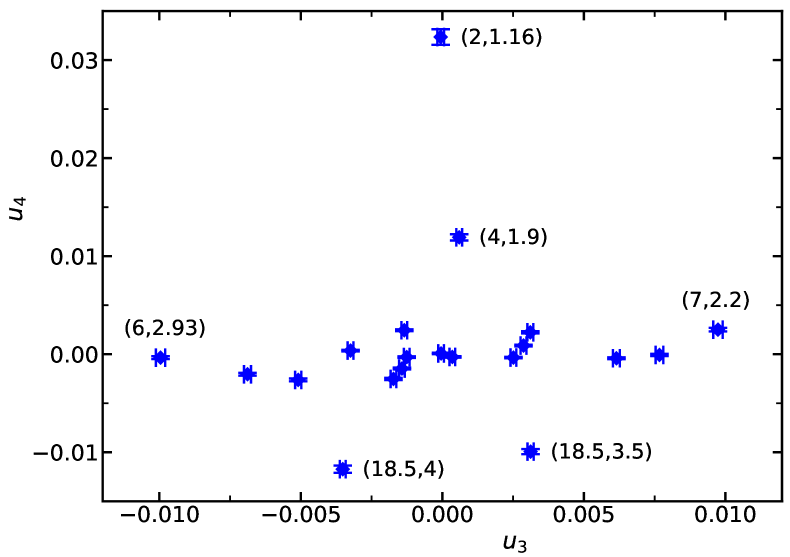
Figure 2: We plot the estimates of the correction amplitudes $(u_{3},u_{4})$ obtained by fitting our data for dimensionless quantities for $N=4$ and $L_{min}=12$ with the Ansatz (35). Each data point corresponds to a pair $(\lambda,\mu)$ we simulated at. To keep the figure readable, we give the values of $(\lambda,\mu)$ only for some data points. The complete information is given in Table 2.

In the case of the other quantities we proceed analogously. We obtain $\omega_{2}=0.082(5)$, $\omega_{1}=0.763(24)$ for the correction exponents. Note that the estimate of $\omega_{1}$ is within errors the same as $\omega=0.755(5)$ obtained for the $O(4)$-symmetric fixed point in Ref. myON . The value of $\omega_{2}$ is clearly smaller than $Y_{4}=0.125(5)$ obtained in O234 , indicating that the approximation discussed in Sec. IV.2 is not appropriate for $N=4$. Our results for the dimensionless quantities are given in Table 3. These clearly differ from the $O(4)$-symmetric counterparts.

Table 3: Values of dimensionless quantities for a $L^{3}$ lattice with periodic boundary conditions for the cubic fixed point for $N=4$. For comparison we give the results obtained in Ref. myON for the $O(4)$ symmetric case.

quantity	$Z_{a}/Z_{p}$	$\xi_{2nd}/L$	$U_{4}$	$U_{C}$
cubic, $N=4$	0.113495(41)	0.56252(11)	1.104522(71)	-0.08869(22)
$O(4)$-symm.	0.11911(2)	0.547296(26)	1.094016(12)	0

Next we consider an Ansatz based on eq. (35), where the scaling fields $u_{3}$ and $u_{4}$ are parameterized as quadratic functions of $\lambda$ and $\mu$

$$u_{j}=a_{j,\lambda,1}(\lambda-\lambda^{*})+a_{j,\mu,1}(\mu-\mu^{*})+\frac{1}{2}a_{j,\lambda,2}(\lambda-\lambda^{*})^{2}+\frac{1}{2}a_{j,\mu,2}(\mu-\mu^{*})^{2}+a_{j,\lambda,\mu}(\lambda-\lambda^{*})(\mu-\mu^{*})\;.$$ (45)

In our Ansatz, $\lambda^{*}$, $\mu^{*}$, and $a_{j,\lambda,1}$, $a_{j,\mu,1}$, $a_{j,\lambda,2}$, $a_{j,\mu,2}$, and $a_{j,\lambda,\mu}$ for both values of $j$ are free parameters.

In order to get an acceptable $\chi^{2}/$DOF we had to restrict the range of $\lambda$ and $\mu$ such that 7 or 8 pairs $(\lambda,\mu)$ remained. Since this way data with a large amplitude of $u_{3}$ and $u_{4}$ are excluded, no accurate estimate of $\omega_{1}$ and $\omega_{2}$ is obtained in the fit. Therefore, we have fixed these to the values obtained above.

In order to get the final estimate we considered the following Ansätze and data sets: Ansatz (35) for $L_{min}=12$ and $16$ and the Ansatz (35) with a term proportional to $L^{-4}$ for $L_{min}=12$. Using these Ansätze we fitted the data set with 7 or 8 pairs $(\lambda,\mu)$. Based on these results, proceeding as discussed above, we arrive at

$$(\lambda,\mu)^{*}=(7.10(15),2.642(26)).$$ (46)

Furthermore get $a_{3,\lambda,1}/a_{3,\mu,1}=-0.180(5)$, Eq. (45), characterizing the line of vanishing $u_{3}$ in the neighborhood of $(\lambda,\mu)^{*}$.

Below we compute the exponents $y_{t}=1/\nu$ and $\eta$ based on our data for $(\lambda,\mu)=(7,2.64)$, which is close to $(\lambda,\mu)^{*}$. In order to estimate errors due to residual correction amplitudes $u_{3}$ and $u_{4}$, we compare with results obtained for $(\lambda,\mu)=(7,3)$ and $(\lambda,\mu)=(18.5,3.5)$ and $(18.5,4)$, respectively. Analyzing our estimates of the correction amplitudes obtained by using the different Ansätze discussed above, we find that $|u_{3}|$ should be at least by a factor of 16 smaller for $(\lambda,\mu)=(7,2.64)$ than for $(\lambda,\mu)=(7,3)$. $|u_{4}|$ should be at least by a factor of 16 smaller for $(\lambda,\mu)=(7,2.64)$ than for $(\lambda,\mu)=(18.5,3.5)$ and $(18.5,4)$.

V.2 The critical exponents $\eta$ and $\nu$

Here we focus on the analysis of our data for $(\lambda,\mu)=(7,2.64)$, which is close to $(\lambda,\mu)^{*}$. In addition, we analyze $(\lambda,\mu)=(7,3)$, $(18.5,3.5)$, and $(18.5,4)$ in order to estimate the possible effect of residual corrections at $(\lambda,\mu)=(7,2.64)$.

V.3 $\eta$ from the FSS behavior of the magnetic susceptibility

We have analyzed our data for the magnetic susceptibility at $(\lambda,\mu)=(7,2.64)$ at either $Z_{a}/Z_{p}=0.113495$ or $\xi_{2nd}/L=0.56252$. We used the Ansätze

$$\bar{\chi}=aL^{2-\eta}+b$$ (47)

or

$$\bar{\chi}=aL^{2-\eta}(1+cL^{-\epsilon})+b\;,$$ (48)

where we have taken either $\epsilon=2.023$ or $4$. Our results are plotted in Fig. 3. Our preliminary estimate $\eta=0.03710(15)$ is chosen such that all four fits are consistent with the estimate for some range of $L_{min}$.

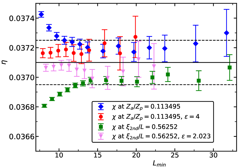
Figure 3: We plot the estimates of $\eta$ obtained by fitting the data for the magnetic susceptibility $\chi$ at $(\lambda,\mu)=(7,2.64)$ and $N=4$ by using the Ansätze (47,48) versus the minimal lattice size $L_{min}$ that is taken into account. The solid line gives our final estimate, while the dashed lines indicate our preliminary error estimate. Note that the values on the $x$-axis are slightly shifted to reduce overlap of the symbols.

In order to estimate the error due to residual correction amplitudes $u_{3}$ and $u_{4}$ at $(\lambda,\mu)=(7,2.64)$, we have analyzed the magnetic susceptibility at $(\lambda,\mu)=(7,3)$, $(18.5,3.5)$, and $(18.5,4)$ by using the same Ansätze as for $(\lambda,\mu)=(7,2.64)$. In the case of $(\lambda,\mu)=(7,3)$, we see a larger spread between the results for $Z_{a}/Z_{p}=0.113495$ and $\xi_{2nd}/L=0.56252$ fixed. For $\xi_{2nd}/L=0.56252$, using Ansatz (47), we get very similar results as for $(\lambda,\mu)=(7,2.64)$. In contrast for $Z_{a}/Z_{p}=0.113495$, using Ansatz (47), we get, for example, $\eta=0.03753(8)$ for $L_{min}=16$.

In the case of $(\lambda,\mu)=(18.5,3.5)$ and $(18.5,4)$, the estimates of $\eta$ are smaller than those for $(\lambda,\mu)=(7,2.64)$ throughout. For example, $\eta=0.03661(12)$ using Ansatz (47) for $L_{min}=20$ and $(18.5,3.5)$, fixing $Z_{a}/Z_{p}=0.113495$.

Given the discussion on the relative amplitude of the scaling fields above, we enlarge the error to

$$\eta=0.0371(2)\;\;,$$ (49)

to take into account the possible effect of residual corrections due to the scaling fields $u_{3}$ and $u_{4}$ at $(\lambda,\mu)=(7,2.64)$. Our estimate clearly differs from $\eta_{O(4)}=0.03624(8)$, Ref. myON for the $O(4)$ symmetric fixed point.

V.4 The thermal RG-exponent $y_{t}=1/\nu$ from the FSS behavior of the slopes of phenomenological couplings

The slope of a dimensionless quantity at the critical point behaves as

$$S_{i}=\frac{\partial R_{i}}{\partial\beta}=a_{i}L^{y_{t}}(1+\sum_{j}b_{i,j}L^{y_{j}}+...)+\sum_{j}c_{i,j}L^{y_{j}}+...\;,$$ (50)

where $b_{i,3}$ and $b_{i,4}$ vanish for an improved model, while $c_{i,3}$ and $c_{i,4}$ are finite.

In order to check the effect of $c_{i,3}L^{y_{3}}$ we can construct linear combinations of dimensionless quantities that do not depend on $u_{3}$. To this end we use the results of the previous section, where we obtained the dependence of $R_{i}$ on $u_{3}$. In particular we have constructed such combinations for either $Z_{a}/Z_{p}$ or $\xi_{2nd}/L$ with $U_{C}$.

We have computed the slopes of dimensionless quantities at either $\xi_{2nd}/L=0.56252$ or $Z_{a}/Z_{p}=0.113495$. We have fitted our data with the Ansatz

$$\bar{S}=aL^{y_{t}}(1+cL^{-\epsilon})\;,$$ (51)

where we take $\epsilon=2.023$, which is the estimate of the exponent related with the violation of the rotational invariance by the lattice. As a check, we performed fits with $\epsilon=2-\eta$, taking our estimate of $\eta$ obtained above. The estimates of $y_{t}$ change only by little. In Fig. 4 we plot the estimates for $Z_{a}/Z_{p}=0.113495$ obtained by fitting the data for $(\lambda,\mu)=(7,2.64)$ taking $\epsilon=2.023$. As preliminary result we obtain $y_{t}=1.3898(7)$. It is chosen such that the estimates obtained by the fits are covered for all four slopes for some range of $L_{min}$. Analyzing the slopes at $\xi_{2nd}/L=0.56252$, we get fully consistent results.

We have repeated this analysis for $(\lambda,\mu)=(7,3)$, $(18.5,3.5)$, and $(18.5,4)$ to see the effect of the corrections on the estimate of $y_{t}$. For $(\lambda,\mu)=(7,3)$ we get essentially consistent results from the different slopes that we consider. We get the estimate $y_{t}\approx 1.396$ being clearly larger than the estimate obtained for $(\lambda,\mu)=(7,2.64)$.

In the case of $(18.5,3.5)$ and $(18.5,4)$ the estimate of $y_{t}$ obtained from the slope of $U_{4}$ is clearly larger than that obtained from the slopes of $Z_{a}/Z_{p}$ and $\xi_{2nd}/L$. Likely this is due to the fact that the effect of a finite scaling field $u_{4}$ is different in the different slopes. On top of this, there is a clear difference between the results of $(18.5,3.5)$ and $(18.5,4)$, which we attribute to the different sign of $u_{3}$ for these two values of $(\lambda,\mu)$. From the slopes of $Z_{a}/Z_{p}$ and $\xi_{2nd}/L$ we get $y_{t}\approx 1.386$ and $1.392$, respectively.

Given the discussion on the relative amplitude of the scaling fields above, we enlarge the error to

$$y_{t}=1.3898(13)$$ (52)

to take into account the possible effect of residual corrections due to the scaling fields $u_{3}$ and $u_{4}$ at $(\lambda,\mu)=(7,2.64)$.

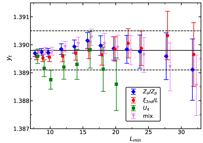
Figure 4: We plot the estimates of $y_{t}$ obtained by fitting the slopes of $Z_{a}/Z_{p}$, $\xi_{2nd}/L$, $U_{4}$ and $Z_{a}/Z_{p}-0.165U_{C}$ at $Z_{a}/Z_{p}=0.113495$ using the Ansatz (51) with $\epsilon=2.023$ versus the minimal lattice size $L_{min}$ that is taken into account. Data for $(\lambda,\mu)=(7,2.64)$ and $N=4$ are analyzed. The dimensionless quantity is given in the legend, where “mix” refers to $Z_{a}/Z_{p}-0.165U_{C}$. The solid line gives our final estimate, while the dashed lines indicate our preliminary error estimate. Note that the values on the $x$ axis are slightly shifted to reduce overlap of the symbols.

VI Critical exponents $Y_{l}$ for $O(3)$ symmetry

We have extended the simulations of Ref. O234 focussing on $N=3$. We make use of the estimate $\lambda^{*}=5.17(11)$ given in the Appendix of myIco . Close to $\lambda^{*}$, the inverse critical temperature is estimated as $\beta_{c}(\lambda=5.0)=0.68756127(13)[6]$ and $\beta_{c}(\lambda=5.2)=0.68798521(8)[3]$.

Here we study the same quantities as in Ref. O234 . We consider perturbations $P_{m,l}$ defined by the power $m$ of the order parameter and the spin representation $l$ of the O($N$) group

$$P_{m,l}^{a_{1}...a_{l}}(\vec{\Phi})=(\vec{\Phi}^{\,2})^{(m-l)/2}Q_{l}^{a_{1}...a_{l}}(\vec{\Phi})\;,$$ (53)

where $Q_{l}^{a_{1}...a_{l}}$ is a homogeneous polynomial of degree $l$ that is symmetric and traceless in the $l$ indices. For $l=4$, see Eq. (5) above. We consider correlators of the type

$$C_{l}=\sum_{a_{1},a_{2},...,a_{l}}\left\langle\sum_{x}Q_{l}^{a_{1},a_{2},...,a_{l}}(\vec{\phi}_{x})\>Q_{l}^{a_{1},a_{2},...,a_{l}}(\vec{m})\right\rangle\;,$$ (54)

where $\vec{M}=\sum_{x}\vec{\phi}_{x}$ and $\vec{m}=\vec{M}/|\vec{M}|$. And in addition

$$D_{l}=\frac{\sum_{a_{1},a_{2},...,a_{l}}\left\langle\sum_{x}Q_{l}^{a_{1},a_{2},...,a_{n}}(\vec{\phi}_{x})\>Q_{l}^{a_{1},a_{2},...,a_{l}}(\vec{M})\right\rangle}{\langle\vec{M}^{\,2}\rangle^{l/2}}\;.$$ (55)

In terms of the angle $\alpha$ between $\vec{m}$ and $\vec{\phi}_{x}$ defined by

$$\vec{\phi}_{x}\cdot\vec{m}=|\vec{\phi}_{x}|\cos(\alpha_{x})$$ (56)

one gets, for example

$$C_{4}=\left\langle\sum_{x}|\vec{\phi}_{x}|^{4}\left(\cos^{4}\alpha_{x}-\frac{6}{N+4}\cos^{2}\alpha_{x}+\frac{3}{(N+2)(N+4)}\right)\right\rangle\;.$$ (57)

The new simulations were in particular designed for $l=4$. Furthermore we have added measurements for $l=5$ and $6$. We notice that the estimators $C_{l}$ and $D_{l}$ become increasingly noisy with increasing $l$. This means that integrated autocorrelation times $\tau_{int}$ go to $0.5$, while the relative variance increases as the lattice size $L$ increases. This behavior can be seen starting from $l=4$. Here we try to attenuate the problem by frequent measurements. To this end, we have implemented local updates, in particular the over-relaxation update efficiently by using AVX intrinsics. See Sec. III.

The most recent update and measurement cycle is

rotate();
for(i=0;i<N_cl;i++) {cluster(0); cluster(1); cluster(2);}
metro(); measure_ene(); measure_X();
for(i=0;i<N_ov;i++) {over(); measure_X();}

rotate() is a global rotation of the field $\phi$ by a random $O(3)$ matrix. cluster(i) is a single-cluster update of the $i^{th}$ component of the field. metro() is the local Metropolis update sweeping over the lattice. At each site an over-relaxation update follows the Metropolis update as second hit. over() is a sweep with the over-relaxation update. measure_ene() is the measurement of the energy, Eq. (10). It remains unchanged under over-relaxation updates. measure_X() is the measurement of the magnetic susceptibility [Eq. (11)] $C_{l}$ and $D_{l}$. In the most recent simulations, we used N_ov $=20$ and N_cl$=L/8$. Some of the simulations for $L<30$ were performed without cluster updates.

We performed simulations at $\lambda=5.2$ and $\beta=0.68798521$ for the linear lattice sizes $L=6$, $7$, …, $28$, $30$, $32$, $36$, $40$ and $48$. In Ref. O234 larger lattice sizes have been simulated. However to get an accurate estimate of $Y_{4}$ it is better to generate high statistics for relatively small lattice sizes.

In the case of our largest linear lattice size $L=48$ we performed $410\;320\;000$ cycles for four copies of the field, while for linear lattice sizes up to $L\approx 20$ about $2\times 10^{9}$ cycles for four copies of the field are performed. Going from $L\approx 20$ up to $L=48$ the statistics gradually decreases.

To check the effect of $\lambda$ on our numerical result we performed simulations at $\lambda=5$ and $\beta=0.68756127$ for linear lattice sizes up to $L=24$.

In total we have used about the equivalent of 20 years of CPU time on a single core of an AMD EPYC^TM 7351P CPU.

VI.1 Analysis of the data

In Fig. 5 we show our estimates obtained for $Y_{2}$ by using the Ansätze

$$C_{l}=aL^{Y_{l}}\;,$$ (58)

$$C_{l}=aL^{Y_{l}}\left(1+bL^{-2+\eta}\right)$$ (59)

and

$$C_{l}=aL^{Y_{l}}\left(1+bL^{-2+\eta}+cL^{-4}\right)\;,$$ (60)

where the term $cL^{-4}$ is an ad hoc choice that is justified by the improved quality of the fits and the fact that for $l=2$, the estimates obtained by using the Ansätze (59,60) are in nice agreement with the result obtained by using the CB method CB_O3 . Analogous fits are performed for $D_{l}$. In general, the results obtained by fitting $D_{l}$ and $C_{l}$ are consistent. The statistical error is slightly smaller for $C_{l}$. Based on fits with the Ansätze (59) and (60), we take $Y_{2}=1.79047(11)$ as preliminary estimate.

As a check we reanalyzed our data for $\lambda=5.2$ at $\beta=0.68798521\pm 0.00000011$, which is our estimate of $\beta_{c}\pm$ the estimate of the error. We find that the estimate of $Y_{2}$ changes by about $2\times 10^{-5}$ with some dependence on the type of the fit and on $L_{min}$. Furthermore, we have replaced $\epsilon_{1}=2-\eta$ by $\epsilon_{1}=2.023$. Also here, the results change by about $2\times 10^{-5}$.

Finally, we estimate the effect of residual leading-order corrections to scaling due to the fact that $\lambda=5.2$ is only an approximation of $\lambda^{*}$. To this end we have simulated the linear lattice sizes $L=10$, $12$, …, $24$ at $\lambda=5.0$ and the estimate of $\beta_{c}$, $\beta=0.68756127$. We computed the ratios $r_{l}(L)=C_{l}(L,\lambda=5.0)/C_{l}(L,\lambda=5.2)$. We have fitted these ratios by using the Ansatz

$$r_{l}(L)=cL^{x}\;.$$ (61)

Taking into account all lattice sizes that we simulated for $\lambda=5.0$ we get $x=0.000138(22)$ for $l=2$. We assume that the difference in the numerical estimate in the exponent is dominated by the difference in the leading correction. Based on the estimate $\lambda^{*}=5.17(11)$, we assume as lower bound $\lambda^{*}\geq 5.06$ in our estimate of the error.

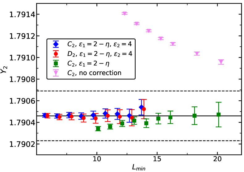
Figure 5: We plot the estimates of $Y_{2}$ for $N=3$ obtained by fitting our data for $C_{2}$ and $D_{2}$ at $\lambda=5.2$ by using the Ansätze (58,59,60). Note that the values on the $x$-axis are slightly shifted to reduce overlap of the symbols. The solid line gives the estimate of Ref. CB_O3 , while the dashed lines indicate the error.

Taking these different errors into account we arrive at the final estimate

$$Y_{2}=1.7905(3)\;.$$ (62)

Performing a similar analysis, we arrive at

$$Y_{3}=0.9615(3)\;.$$ (63)

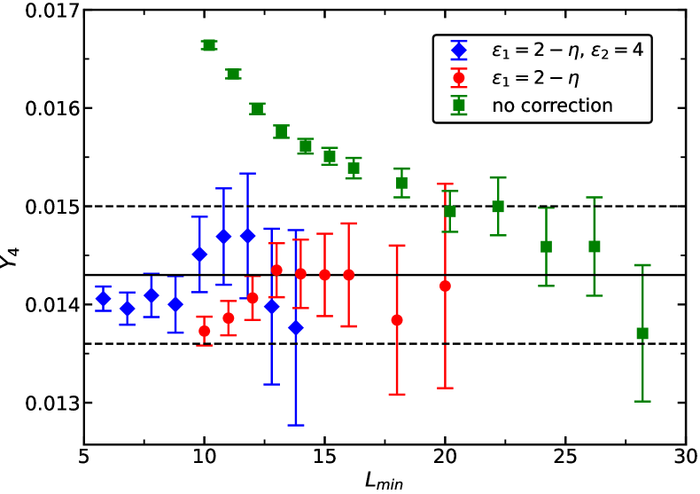
Figure 6: We plot the estimates of $Y_{4}$ obtained by fitting our data for $C_{4}$ at $\lambda=5.2$ for $N=3$ by using the Ansätze (58,59,60). Note that the values on the $x$-axis are slightly shifted to reduce overlap of the symbols. The solid line gives our preliminary estimate of $Y_{4}$, while the dashed lines indicate the error.

In Fig. 6 we plot results obtained for $Y_{4}$. As preliminary estimate we take $Y_{4}=0.0143(7)$. Taking into account systematic errors as discussed above for $l=2$, we arrive at the final estimate

$$Y_{4}=0.0143(9)\;.$$ (64)

In a similar fashion we arrive at $Y_{5}=-1.04(1)$ and $Y_{6}=-2.2(2)$. We notice that the error rapidly increases with increasing $l$. For $l\geq 5$ alternative approaches are likely more suitable. See for example Refs. DebasishO2 ; DebasishO4 .

In these simulations we also have computed the magnetic susceptibility $\chi$. Just as a check, we have fitted the data for $\lambda=5.2$ with the Ansatz

$$\chi=aL^{2-\eta}+b\;.$$ (65)

We get an acceptable goodness of the fit starting from $L_{min}=8$. Estimates of the exponent are for example $\eta=0.037935(15)$, $0.037890(20)$, $0.037881(26)$, $0.037894(35)$, $0.037864(45)$, for $L_{min}=8$, $10$, $12$, $14$, and $16$. Starting from $L_{min}=10$ these estimates are consistent with $\eta=0.037884(102)$ CB_O3 and $\eta=0.03784(5)$ myIco .

VII Simulations and analysis of the data for $N=3$

We simulated at values of $\lambda$ that are close to $\lambda^{*}=5.17(11)$ of the $O(3)$-symmetric case $\mu=0$ myIco . In particular, we simulated the model at $\lambda=5.2$, $\mu=-0.5$, $-0.3$, $-0.1$, $0.05$, $0.1$, $0.2$, $0.3$, $0.4$, $0.5$, and $0.7$ using $L_{max}=48$, $48$, $48$, $48$, $48$, $48$, $200$, $48$, $48$, $48$, respectively. Furthermore, we simulated at $\lambda=5$, $\mu=-0.3$, $-0.1$, $0.1$, $0.2$, $0.25$, $0.3$, and $0.4$, using $L_{max}=96$, $48$, $48$, $48$, $100$, $200$, and $48$, respectively, at $\lambda=4.8$, $\mu=-0.5$, $-0.3$, $0.2$, $0.3$, $0.4$, and $0.5$, using $L_{max}=64$, $48$, $48$, $200$, $48$, and $64$, respectively, at $\lambda=4.7$, $\mu=-0.7$, and $0.7$ using $L_{max}=64$, at $\lambda=4.5$, $\mu=-1.0$, $-0.5$, $-0.3$, $-0.15$, $0.15$, $0.25$, $0.3$, $0.35$, $0.5$ and $1.0$, using $L_{max}=64$, $32$, $32$, $32$, $32$, $32$, $32$, $32$, $32$, and $64$, respectively, and at $\lambda=4.3$, $\mu=-1.0$ using $L_{max}=64$. Here, $L_{max}$ is the largest linear lattice size that we simulated.

For example for $(\lambda,\mu)=(5.0,0.3)$, which is close to $(\lambda,\mu)^{*}$ as we shall see below, we simulated the linear lattice sizes $L=8$, $9$, …, $16$, $18$, …, $36$, $40$, …, $48$, $56$, $60$, $64$, $72$, $80$, $90$, $100$, $110$, $120$, $140$, and $200$. We performed about $2\times 10^{9}$ measurements for each lattice size up to $L=24$. Then the number of measurements gradually drops. For example, we performed $8.6\times 10^{8}$, $1.2\times 10^{8}$, and $2.1\times 10^{7}$ measurements for $L=48$, $100$, and $200$, respectively. The simulations at $(\lambda,\mu)=(5.0,0.3)$ took about the equivalent of 25 years of CPU time on a single core of an AMD EPYC^TM 7351P CPU. All simulations for $\mu\neq 0$ took about the equivalent of 130 years of CPU time on a single core of an AMD EPYC^TM 7351P CPU.

In addition we used the data for $\mu=0$, $\lambda=5.0$ and $5.2$, discussed in the Appendix A of Ref. myIco . We have added the lattice sizes $L=32$, $48$, $56$, $64$, and $72$ for $\lambda=5.0$ and $L=32$, $48$, $56$, $64$, $72$ and $90$ for $\lambda=5.2$ to have a better match with the lattice sizes simulated for $\mu\neq 0$.

Note that here we have simulated also negative values of $\mu$, where a first order transition is expected. However for the values of $\mu$ studied here, the linear lattice size $L$ should be smaller by several orders than the correlation length at the transition. Therefore, it is justified to treat the systems as if they were critical.

VII.1 dimensionless quantities

As for $N=4$, we first analyze the behavior of dimensionless quantities. In a first series of fits, we use Ansätze, where we expand around the $O(3)$-symmetric fixed point. For the dimensionless quantities $Z_{a}/Z_{p}$, $\xi_{2nd}/L$ and $U_{4}$ we take

$$R_{i}(\beta_{c},\lambda,\mu,L)=R_{i}^{*}+r_{i,4}w_{4}(\lambda,\mu)L^{-\omega}+\sum_{m=2}^{m_{max}}c_{i,m}U_{C}^{m}(\beta_{c},\lambda,\mu,L)+\sum_{j}a_{i,j}L^{-\epsilon_{j}}\;,$$ (66)

where $\epsilon_{j}\gtrapprox 2$. Equation (66) is a standard Ansatz for analyzing dimensionless quantities at $\mu=0$, augmented by $\sum_{m=2}^{m_{max}}c_{i,m}U_{C}^{m}(\beta_{c},\lambda,\mu,L)$. The basic idea of the Ansatz is that $Z_{a}/Z_{p}$, $\xi_{2nd}/L$ and $U_{4}$ behave as $R_{i}(\beta_{c},\lambda,\mu,L)=R_{i}(\beta_{c},\lambda,0,L)+O(\mu^{2})$, while $U_{C}=O(\mu)$, due to symmetry. Hence $R_{i}^{*}$ are the $O(3)$-symmetric fixed point values. Here we avoid an explicit parameterization of the RG flow of the cubic perturbation. Instead, we take it from the dimensionless quantity $U_{C}$. In our fits, we chose either $m_{max}=3$, $4$, or $5$. The term $r_{i,4}w_{4}(\lambda,\mu)L^{-\omega}$ is an approximation based on the fact that $\omega_{1}\gg Y_{4},\omega_{2}$. In the approximation we assume a line of fixed points, and furthermore that the correction exponent $\omega_{1}$ stays constant along this line.

In order to fix the normalization of $w_{4}(\lambda,\mu)$, we set $r_{U_{4},4}=1$ for the Binder cumulant $U_{4}$. The choice of subleading corrections depends on the dimensionless quantity. In the case of $Z_{a}/Z_{p}$ we take $\epsilon=2.023$, which is an estimate of the correction exponent related with the violation of rotational invariance by the lattice. The amplitude $a_{Z_{a}/Z_{p},1}$ is assumed to be constant in $\lambda$ and $\mu$. In the case of $\xi_{2nd}/L$, we take two correction terms, one with the correction exponent $\epsilon_{1}=2-\eta$, associated with the analytic background of the magnetic susceptibility, and, as for $Z_{a}/Z_{p}$, one with the correction exponent $\epsilon_{2}=2.023$. The amplitude $a_{\xi_{2nd}/L,2}$ is assumed to be constant in $\lambda$ and $\mu$. The amplitude $a_{\xi_{2nd}/L,1}$ is parameterized as linear in $\lambda$ and quadratic in $\mu$. We experimented with various dependencies on $\lambda$ and $\mu$, which however did not improve the quality of the fit. In the case of $U_{4}$, we take one correction term with $\epsilon_{1}=2-\eta$. The amplitude $a_{U_{4},1}$ is parameterized as $a_{\xi_{2nd}/L,1}$. As check, we added a second correction term with $\epsilon_{2}=2.023$ in some of the fits. We performed fits fixing $\omega=0.759$, which is the value obtained for the $O(3)$-symmetric fixed point myIco . For technical reasons, we ignore the statistical error of $U_{C}(\beta_{s},\lambda,\mu,L)$ and the Taylor coefficients in $(\beta_{c}-\beta_{s})$. This is justified by the fact that $\sum_{m=2}^{m_{max}}c_{i,m}U_{C}(\beta_{c},\lambda,\mu,L)^{m}$ assumes only rather small values. As check, we added a term proportional to $L^{-4}$ for each dimensionless quantity, were the amplitudes are constant in $\mu$ and $\lambda$. In a first series of fits, we used $w_{4}(\lambda,\mu)$ as a free parameter for each pair $(\lambda,\mu)$.

Fitting the data for $|\mu|\leq 0.5$ with the Ansatz (66) and $m_{max}=3$, we get $\chi^{2}/$DOF$=1.125$, $1.076$, $1.086$ and $1.066$ corresponding to $p=0.002$, $0.056$, $0.057$, and $0.13$ for $L_{min}=12$, $16$, $20$, and $24$, respectively. Adding a term proportional to $L^{-4}$ for each dimensionless quantity, we get $\chi^{2}/$DOF $=1.061$, $1.074$, $1.075$, and $1.061$ corresponding to $p=0.078$, $0.062$, $0.084$, and $0.148$ for $L_{min}=12$, $16$, $20$, and $24$, respectively. Fitting the data for $|\mu|\leq 0.7$ with the Ansatz (66) and $m_{max}=3$, the $p$-value is smaller than $0.1$ for $L_{min}<24$, while for $L_{min}=24$ we get $\chi^{2}/$DOF $=1.071$ corresponding to $p=0.106$. Adding a term proportional to $L^{-4}$ for each dimensionless quantity the fits for $L_{min}<24$ are worse than those for $|\mu|\leq 0.5$, while for $L_{min}=24$ we get $\chi^{2}/$DOF $=1.068$ corresponding to $p=0.116$.

Fitting the data for $|\mu|\leq 1.0$ with the Ansatz (66) and $m_{max}=3$, for $L_{min}=24$ we get $\chi^{2}/$DOF $=1.471$ corresponding to $p=0.000$. Adding a term proportional to $L^{-4}$ for each dimensionless quantity, the quality of the fit does not improve considerably.

Fitting the data for $|\mu|\leq 1.0$ with the Ansatz (66) and $m_{max}=4$, the quality of the fit improves considerably. We get $\chi^{2}/$DOF $=1.111$, $1.065$, $1.078$, and $1.051$, corresponding to $p=0.004$, $0.077$, $0.066$, and $0.179$ for $L_{min}=12$, $16$, $20$, and $24$, respectively. Adding a term proportional to $L^{-4}$ for each dimensionless quantity, we get $\chi^{2}/$DOF $=1.050$, $1.063$, $1.070$, and $1.047$, corresponding to $p=0.112$, $0.082$, $0.087$, and $0.198$ for $L_{min}=12$, $16$, $20$, and $24$, respectively. Going from $m_{max}=4$ to $m_{max}=5$, taking into account the data with $|\mu|\leq 1.0$, the quality of the fits only slightly improves.

We conclude that our approximative Ansatz (66), for our high statistics data, is at the edge of being acceptable, which in the literature is usually assumed to be the case for $0.1\leq p\leq 0.9$. For $|\mu|\leq 0.5$, $m_{max}=3$ seems to be sufficient, while for $|\mu|\leq 1$ at least one more power of $U_{C}$ has to be added.

In Table 4 we give a few characteristic results for the dimensionless quantities obtained by using these fits. These are consistent with those of Ref. myIco . A more accurate final result than that given in Ref. myIco can not be obtained.

Table 4: Estimates of the fixed point values $R^{*}$ of dimensionless quantities $R$ at the $O(3)$-invariant fixed point. These are obtained by using the Ansatz (66). In the last line we give the final results of Ref. myIco for comparison. For a discussion see the text.

$m_{max}$	$L^{-4}$	range	$L_{min}$	$(Z_{a}/Z_{p})^{*}$	$(\xi_{2nd}/L)^{*}$	$U_{4}^{*}$
3	no	$|\mu|\leq 0.5$	24	0.194766(13)	0.564036(11)	1.139284(10)
3	yes	$|\mu|\leq 0.5$	12	0.194753(7)	0.564051(6)	1.139299(6)
4	no	$|\mu|\leq 1.0$	24	0.194761(11)	0.564041(10)	1.139289(9)
4	yes	$|\mu|\leq 1.0$	12	0.194750(6)	0.564053(5)	1.139300(5)
ref. myIco				0.19477(2)	0.56404(2)	1.13929(2)

Next we consider the coefficients $c_{i,m}$. As final result we quote numbers that are consistent with four different fits. First we took $m_{max}=4$ and data for $|\mu|\leq 0.7$. Using a correction term proportional to $L^{-4}$ we took the result for $L_{min}=12$, while without this correction the data are taken for $L_{min}=24$. The third and fourth fit are analogous, but for $m_{max}=5$ and data for $|\mu|\leq 1.0$. We get $c_{Z_{a}/Z_{p},2}=-0.64(5)$, $c_{Z_{a}/Z_{p},3}=2.1(3)$, $c_{\xi_{2nd}/L,2}=1.34(4)$, $c_{\xi_{2nd}/L,3}=-3.4(3)$, $c_{U_{4},2}=1.25(3)$, and $c_{U_{4},3}=-3.0(3)$. Coefficients for $m=4$ and $5$ have large error bars and vary considerably among the different fits.

In the approximation used in the fits discussed in this section, there is an improved line $\lambda^{*}(\mu)$, where the correction proportional to $L^{-\omega}$ vanishes. We have computed zeros of $w_{4}(\lambda,\mu)$ for given $\mu$ by linear interpolation in $\lambda$. Our final results, which are consistent with the four different fits used above are given in table 5. The maximum of $\lambda^{*}(\mu)$ is reached for $\mu=0$. The result for $\lambda^{*}(0)$ is consistent with $\lambda^{*}=5.17(11)$ obtained in ref. myIco . $\lambda^{*}(\mu)$ is almost even in $\mu$. $\lambda^{*}(\mu)$ for negative values of $\mu$ is slightly smaller than for the corresponding positive values of $\mu$.

Table 5: Numerical results for $\lambda^{*}(\mu)$ for $N=3$. For a discussion see the text.

$\mu$	$\lambda^{*}$
-0.7	4.53(22)
-0.5	4.78(13)
-0.3	4.97(10)
-0.1	5.08(10)
0.0	5.10(10)
0.1	5.09(10)
0.2	5.04(10)
0.3	4.98(10)
0.4	4.90(10)
0.5	4.81(13)
0.7	4.55(22)

Next we used the parameterization for the correction amplitude

$$w_{4}(\lambda,\mu)=a(\lambda-\lambda^{*}-c\mu^{2}-d\mu^{3})\;(1+e(\lambda-5.0))$$ (67)

and

$$w_{4}(\lambda,\mu)=a(\lambda-\lambda^{*}-c\mu^{2}-d\mu^{3}-e\mu^{4})\;(1+f(\lambda-5.0))\;,$$ (68)

where we have added one term proportional to $\mu^{4}$. We obtain a similar quality of the fit as above without parameterization of $w_{4}(\lambda,\mu)$. Also the differences between the two parameterizations (67, 68) is minor. Therefore we abstain from a detailed discussion. Let us just briefly summarize the results for the parameters of Eqs. (67) and (68) and the estimate of $\beta_{c}$ that we obtain.

To this end let us discuss the results of four selected fits

• For the Ansatz (66) without a correction of $U_{4}$ proportional to $L^{-2.023}$ and no correction proportional to $L^{-4}$, $m_{max}=5$, the parameterization (67), $|\mu|\leq 1$, and $L_{min}=24$ we get $\chi^{2}/$DOF $=1.052$ corresponding to $p=0.168$. The estimates of the parameters are $\lambda^{*}=5.14(4)$, $c=-1.17(17)$, and $d=0.07(1)$.

• For the Ansatz (66) without a correction of $U_{4}$ proportional to $L^{-2.023}$, no correction proportional to $L^{-4}$, $m_{max}=5$, the parameterization (68), $|\mu|\leq 1$, and $L_{min}=24$ we get $\chi^{2}/$DOF $=1.051$ corresponding to $p=0.171$. The estimates of the parameters are $\lambda^{*}=5.15(4)$, $c=-1.24(18)$, $d=0.05(3)$, and $e=0.07(6)$.

• For the Ansatz (66) with a correction of $U_{4}$ proportional to $L^{-2.023}$, no correction proportional to $L^{-4}$, $m_{max}=5$, the parameterization (68), $|\mu|\leq 1$, and $L_{min}=16$ we get $\chi^{2}/$DOF $=1.044$ corresponding to $p=0.159$. The estimates of the parameters are $\lambda^{*}=5.13(6)$, $c=-0.78(7)$, $d=0.05(1)$, and $e=0.04(3)$.

• For the Ansatz (66) without a correction of $U_{4}$ proportional to $L^{-2.023}$, but a correction proportional to $L^{-4}$ for all dimensionless quantities, $m_{max}=5$, the parameterization (68), $|\mu|\leq 1$, and $L_{min}=12$ we get $\chi^{2}/$DOF $=1.041$ corresponding to $p=0.156$. The estimates of the parameters are $\lambda^{*}=5.096(20)$, $c=-0.78(4)$, $d=0.05(1)$, and $e=0.04(2)$.

In summary, also taking into account fits not explicitly given above, we find values of $\lambda^{*}$ that are consistent with $\lambda^{*}=5.17(11)$ obtained in Ref. myIco . Furthermore $-1.5\lessapprox c\lessapprox-0.7$, where the smaller values of $c$ are correlated with larger values of $\lambda^{*}$. There is only a small asymmetry in $\mu$, corresponding to small values of $d$. These findings are consistent with the results for $\lambda^{*}(\mu)$, which are summarized in table 5.

Finally in tables 6 and 7 we give the results for $\beta_{c}$ which are based on the four fits which are explicitly discussed above. Given the large number of pairs $(\lambda,\mu)$ we simulated at, we used an automated procedure to obtain the central value and its error, similar to the analysis for $N=4$ above. These results might be used to bias the analysis of high temperature (HT) series expansions or in future Monte Carlo studies of the model.

Table 6: Numerical results for the inverse critical temperature $\beta_{c}$ for the pairs of $(\lambda,\mu)$ we simulated at for $N=3$. For a discussion see the text.

$\lambda$	$\mu$	$\beta_{c}$
4.3	-1.00	0.6773490(14)
4.5	-1.00	0.67841424(96)
4.5	-0.50	0.68439865(37)
4.5	-0.30	0.68559135(40)
4.5	-0.15	0.68607863(25)
4.5	0.15	0.68608422(22)
4.5	0.25	0.68581697(32)
4.5	0.30	0.68563593(23)
4.5	0.35	0.68542342(26)
4.5	0.50	0.68460540(23)
4.5	1.00	0.68006803(59)

Table 7: Continuation of table 6.

$\lambda$	$\mu$	$\beta_{c}$
4.7	-0.70	0.68329292(59)
4.7	0.70	0.68382797(22)
4.8	-0.50	0.68536469(28)
4.8	-0.30	0.68647819(18)
4.8	0.20	0.68682876(15)
4.8	0.30	0.68651908(10)
4.8	0.40	0.68609278(13)
4.8	0.50	0.68555428(13)
5.0	-0.30	0.68698276(13)
5.0	-0.10	0.68749850(13)
5.0	0.00	0.68756126(8)
5.0	0.10	0.68749982(12)
5.0	0.20	0.68731855(11)
5.0	0.25	0.68718435(9)
5.0	0.30	0.68702161(6)
5.0	0.40	0.68661260(11)
5.2	-0.50	0.68640695(35)
5.2	-0.30	0.68742991(35)
5.2	-0.10	0.68792511(14)
5.2	0.00	0.68798524(8)
5.2	0.05	0.68797037(15)
5.2	0.10	0.68792634(12)
5.2	0.20	0.68775221(10)
5.2	0.30	0.68746677(11)
5.2	0.40	0.68707374(14)
5.2	0.50	0.68657694(16)
5.2	0.70	0.68528562(32)

VII.1.1 $U_{C}$ at $Z_{a}/Z_{p}=0.19477$

In a complementary analysis we considered $U_{C}$ at $Z_{a}/Z_{p}=0.19477$. To get a first impression of its behavior, we plot $\bar{U}_{C}$ as a function of the linear lattice size $L$ for $(\lambda,\mu)=(5.0,0.2)$ and $(5.0,0.4)$ in Fig. 7. We find that $\bar{U}_{C}$ is slowly decreasing with increasing lattice size for $\mu=0.2$, while it is increasing for $\mu=0.4$. We notice that high statistical accuracy is needed to detect this behavior. We expect that $0.2<\mu^{*}<0.4$. For $\mu<0$, $\bar{U}_{C}$ is positive and it is increasing with increasing lattice size, throughout.

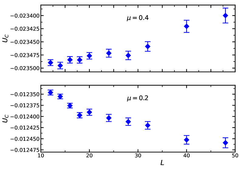
Figure 7: We plot $U_{C}$ at $Z_{a}/Z_{p}=0.19477$ versus the linear lattice size $L$ for $\lambda=5.0$ and $N=3$. In the upper part we give numerical results for $\mu=0.4$ and in the lower part the estimates for $\mu=0.2$.

Let us analyze $\bar{U}_{C}$ quantitatively. We performed joint fits for different values of $\mu$ and a single value of $\lambda$, either $\lambda=4.8$, $5.0$ or $\lambda=5.2$.

First we performed fits by using the Ansatz (44)

$$\bar{U}_{C}(\mu,\lambda,L)=\frac{\bar{U}_{C}^{*}}{1+q\left(\frac{\mu^{*}}{\mu}-1\right)L^{-y}}\;,$$ (69)

where we simply have replaced $U_{C}$ by $\bar{U}_{C}$. Next we introduce a quadratic correction in $\mu$:

$$\bar{U}_{C}(\mu,\lambda,L)=\frac{\bar{U}_{C}^{*}}{1+q\left(\frac{\bar{\mu}}{\mu+s\mu^{2}}-1\right)L^{-y}}\;,$$ (70)

where now

$$\mu^{*}=\frac{\sqrt{1+4\bar{\mu}s}-1}{2s}$$ (71)

or a correction proportional to $L^{-2+\eta}$

$$\bar{U}_{C}(\mu,\lambda,L)=\frac{\bar{U}_{C}^{*}}{1+q\left(\frac{\mu^{*}}{\mu}-1\right)L^{-y}}\left(1+cL^{-2+\eta}\right)\;.$$ (72)

and both types of corrections

$$\bar{U}_{C}(\mu,\lambda,L)=\frac{\bar{U}_{C}^{*}}{1+q\left(\frac{\bar{\mu}}{\mu+s\mu^{2}}-1\right)L^{-y}}\left(1+cL^{-2+\eta}\right)\;.$$ (73)

We find that acceptable fits can only be obtained by restricting the range of the parameter: $|\mu|\leq 0.4$. In the case of $\lambda=5.0$ we get, by using the Ansatz (73) a $\chi^{2}/$DOF $=1.01$ for $L_{min}=12$ and $\chi^{2}/$DOF slightly smaller than one for larger $L_{min}$. We obtain $\bar{U}_{C}^{*}=-0.0176(3)$, $-0.0172(4)$, $-0.0171(5)$, $-0.0168(6)$, and $-0.0166(7)$ for $L_{min}=12$, $14$, $16$, $18$, and $20$, respectively. Furthermore $y=0.0149(3)$, $0.0146(4)$, $0.0144(5)$, $0.0142(5)$, and $0.0141(6)$ for the same values of $L_{min}$ as above. Note that $y=Y_{4}=\omega_{2}$ in the approximation used here. For the fixed point value of the parameter $\mu$ we get $\mu^{*}=0.290(6)$, $0.283(8)$, $0.283(9)$, $0.277(11)$, and $0.273(12)$.

Comparing with the results obtained by using the other Ansätze and $\lambda=4.8$ and $5.2$ we arrive at the final results

$$Y_{4}=0.0144(15)$$ (74)

and

$$\bar{U}_{C}^{*}=-0.017(2)\;.$$ (75)

The error bars are chosen such that the estimates of different acceptable fits are covered. For $\lambda=5.0$ we conclude $\mu^{*}=0.28(2)$. The estimates for $\lambda=4.8$ and $5.2$ are the same within errors.

We have repeated the analysis for $U_{C}$ at $Z_{a}/Z_{p}-0.64U_{C}^{2}+2.1U_{C}^{3}=0.19477$. We arrive at very similar results. (Revised version: See remark in Sec. VII.1.3).

Putting things together, the improved model for the cubic fixed point is given by $(\lambda,\mu)^{*}_{cubic}=(4.99(11),0.28(2))$, where we obtain the value of $\lambda$ by interpolating the estimates for $\mu=0.2$ and $0.3$ given in table 5.

We performed fits with Ansätze that combine Eq. (66) with the Ansätze for $U_{C}$ discussed in this subsection. The results are fully consistent with those given above. Therefore we abstain from a discussion.

VII.1.2 Generic Ansatz for the dimensionless quantities in the neighborhood of the cubic fixed point

Finally we performed fits, similar to the case $N=4$, with a generic Ansatz, not exploiting the vicinity of the $O(3)$ symmetric fixed point. In order to get an acceptable $\chi^{2}/$DOF, using the parameterization (45), the values of $(\lambda,\mu)$ have to be restricted to a close neighborhood of $(\lambda,\mu)^{*}$. Here we only included data with $0.2\leq\mu\leq 0.4$ for $\lambda=4.8$, $5.0$, and $5.2$. We are aiming at estimates of the fixed point values of the dimensional quantities $R_{i}^{*}$ and $(\lambda,\mu)^{*}$.

First we take $\omega_{2}$ as free parameter in the Ansatz (35), while we fix $\omega_{1}=0.759$ myIco . We get an acceptable goodness of the fit starting from $L_{min}=18$. We get $\omega_{2}=0.0150(13)$, $0.0137(17)$, $0.0179(23)$, and $0.021(3)$ for $L_{min}=12$, $14$, $16$, and $18$. Going to larger values of $L_{min}$, the statistical error is rapidly increasing. Therefore we performed fits fixing $\omega_{2}=0.0143$. In this case, we also get an acceptable goodness of the fit starting from $L_{min}=18$. As a check, we also performed fits using $\omega_{2}=0.013$, taking into account possible deviations of $\omega_{2}$ from $Y_{4}$ of the $O(3)$-invariant fixed point.

We arrive at $(\lambda,\mu)^{*}_{cubic}=(4.98(10),0.30(3))$ covering results for $L_{min}=18$ up to $24$. The differences of results for $\omega_{2}=0.013$ and $0.0143$ are clearly smaller than the error bars quoted.

Furthermore we get

$$(Z_{a}/Z_{p})^{*}_{cubic} = 0.19453(5)$$ (76)

$$(\xi_{2nd}/L)^{*}_{cubic} = 0.56451(7)$$ (77)

$$U_{4,cubic}^{*} = 1.13972(6)$$ (78)

$$U_{C,cubic}^{*} = -0.0181(12)$$ (79)

for the cubic fixed point. Also here, the estimates for $L_{min}=18$ up to $L_{min}=24$ are covered and the difference of results for $\omega_{2}=0.013$ and $0.0143$ are clearly smaller than the error bars quoted.

The estimates of $(Z_{a}/Z_{p})^{*}_{cubic}$, $(\xi_{2nd}/L)^{*}_{cubic}$ and $U^{*}_{4,cubic}$ differ only slightly from the values for the $O(3)$ symmetric fixed point. However the differences are clearly larger than the error estimates.

VII.1.3 Flow equation for $\bar{U}_{C}$

Finally we consider the dimensionless quantity $U_{C}$ itself as coupling. In order to stay at criticality we take it at $Z_{a}/Z_{p}-0.64U_{C}^{2}+2.1U_{C}^{3}=0.19477$.

(Remark revised version: $Z_{a}/Z_{p}-0.64U_{C}^{2}+2.1U_{C}^{3}$ should be $Z_{a}/Z_{p}+0.64U_{C}^{2}-2.1U_{C}^{3}$. However even with the wrong sign it is a dimensionless quantity that can be fixed to a certain value. Errors in the final result might become larger due to larger corrections. However, we have checked that replacing $-0.64U_{C}^{2}+2.1U_{C}^{3}$ by $+0.64U_{C}^{2}-2.1U_{C}^{3}$ changes virtually nothing in the final results. Therefore we did not update the discussion of the analysis of the data below.)

Furthermore we stay, at the level of our numerical precision, on the line $\lambda^{*}(\mu)$.

We determine

$$u=\frac{1}{\bar{U}_{C}}\frac{\mbox{d}\bar{U}_{C}}{\mbox{d}l}\;,$$ (80)

where $l=\ln L$, by fitting the data for fixed $(\lambda,\mu)$ by using the Ansatz

$$\bar{U}_{C}(\lambda,\mu,L)=aL^{u}$$ (81)

for some range $L_{min}\leq L\leq L_{max}$. As argument of $u$ we take $[\bar{U}_{C}(L_{min})+\bar{U}_{C}(L_{max})]/2$. The approximation (81) relies on the fact that $\bar{U}_{C}$ varies only little in the range of linear lattice sizes considered. In order to check the effect of subleading corrections, we consider different ranges $L_{min}\leq L\leq L_{max}$. For $L_{min}=32$ the maximal lattice size $L_{max}$ is determined by the largest lattice size that we have simulated. For $L_{min}=16$ and $24$, we reduce $L_{max}$ by the corresponding factor with respect to $L_{min}=32$. Finally we used the Ansatz

$$\bar{U}_{C}(\lambda,\mu,L)=aL^{u}\;(1+cL^{-2})$$ (82)

with $L_{min}=12$ and $L_{max}$ given by the largest lattice size simulated. In our analysis, we took into account the data for $(\lambda,\mu)=(4.3,-1)$, $(4.5,-1)$, $(4.7,-0.7)$, $(4.8,-0.5)$, $(5.0,-0.3)$, $(5.0,-0.1)$, $(5.2,-0.1)$, $(5.0,0.1)$, $(5.2,0.1)$, $(5.0,0.2)$, $(5.2,0.2)$, $(5.0,0.25)$, $(5.0,0.3)$, $(5.0,0.4)$, $(4.8,0.5)$, $(4.7,0.7)$, and $(4.5,1.0)$.

We fit the estimates of $u$ by using the Ansatz

$$u(\bar{U}_{C})=a+b\bar{U}_{C}+c\bar{U}_{C}^{2}+d\bar{U}_{C}^{3}$$ (83)

and as check

$$u(\bar{U}_{C})=a+b\bar{U}_{C}+c\bar{U}_{C}^{2}\;.$$ (84)

It turns out that the Ansatz (84) gives quite large $\chi^{2}/$DOF, when all data are fitted, while Ansatz (83) results in an acceptable $\chi^{2}/$DOF. Excluding the data for $|\mu|=1$, also Ansatz (84) gives acceptable values of $\chi^{2}/$DOF.

In Fig. (8) we plot the numerical estimates of $u(\bar{U}_{c})$ obtained by using the Ansatz (82) with $L_{min}=12$. The line corresponds to the fit of the data by using the Ansatz (83). The relative error of the data for $|\mu|\leq 0.2$ is large. These data contribute little to the final result.

In table 8 we summarize the numerical results. In addition to the estimates of the parameters of the Ansätze (83,84) we give the zero $\bar{U}_{C}^{*}$ of $u$ and the correction exponent $\omega_{2}$ at this zero. These are computed numerically for the given estimates of $a$, $b$, $c$ and $d$.

Table 8: Results of fitting $u(\bar{U}_{c})$ by using the Ansatz (83) or  (84). The estimates of $u$ are obtained by using the Ansatz (81) or (82) using the minimal lattice size $L_{min}$. The corresponding maximal lattice size is given in the text. $a$, $b$, $c$ and $d$ are the parameters of the Ansätze (83,84). If no value for $d$ is given, Ansatz (84) is used. Otherwise the data are fitted by using the Ansatz (83). $\bar{U}_{C}^{*}$ is the zero of $u$ that is computed numerically and $\omega_{2}$ the correction exponent at this zero. (Remark revised version: by mistake we have computed the statistical error of $a+\omega_{2}$ instead of $a-\omega_{2}$. The error of $a-\omega_{2}$ is smaller than that of $a+\omega_{2}$. In the table below, still the wrong error is quoted.)

Ansatz	$L_{min}$	a	b	c	d	$\bar{U}_{C}^{*}$	$\omega_{2}$	$a-\omega_{2}$
81	16	0.01558(22)	0.836(6)	2.00(13)	-11.9(1.4)	-0.0197(3)	0.01463(25)	0.00096(32)
81	24	0.01398(41)	0.843(10)	2.64(30)	-17.7(2.9)	-0.0177(5)	0.01296(46)	0.00102(47)
81	32	0.01521(48)	0.826(12)	0.94(16)	-	-0.0188(5)	0.01488(51)	0.00033(53)
81	32	0.01429(55)	0.851(14)	2.06(35)	-12.2(3.4)	-0.0176(6)	0.01352(60)	0.00077(78)
82	12	0.01465(30)	0.848(9)	1.20(16)	-	-0.0177(3)	0.01427(33)	0.00038(34)
82	12	0.01392(31)	0.850(8)	2.20(20)	-10.7(2.1)	-0.0172(4)	0.01316(34)	0.00076(43)

The results obtained by using the Ansatz (81) with $L_{min}=24$ and $32$ and those obtained by using the Ansatz (82) and $L_{min}=12$ are essentially consistent. Fitting $u(\bar{U}_{c})$ by using the Ansatz (83), the results for $a$ are slightly smaller than by using the Ansatz (84). Furthermore, the difference $a-\omega_{2}$ is smaller when fitting by using the Ansatz (84) than for Ansatz (83). Giving preference to the Ansatz (83) and fitting all data, we arrive at the results $Y_{4}=a=0.0142(6)$, $\omega_{2}=0.0133(8)$, and $\bar{U}_{C}^{*}=-0.0175(7)$. Throughout the fits reported in table 8, $\omega_{2}<Y_{4}$, and $Y_{4}-\omega_{2}<0.0015$ in the extreme case, taking into account the statistical error. The estimates of $Y_{4}$ and $\bar{U}_{C}^{*}$ are consistent with those obtained in previous sections.

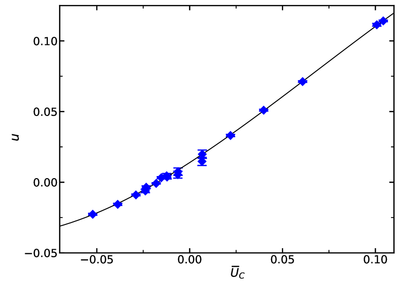
Figure 8: We plot $u\approx\frac{1}{\bar{U}_{C}}\frac{\mbox{d}\bar{U}_{C}}{\mbox{d}l}$ for $N=3$ as a function of $\bar{U}_{c}$. Here we give the data obtained by using the Ansatz (82) and $L_{min}=12$. The line gives the result of the fit with the Ansatz (84).

VII.2 The critical exponent $\eta$

(Remark revised version: Also here the wrong sign of corrections in $U_{C}$ is taken. However a reanalysis, taking the correct sign, or abstain from using it, shows that the final result for $\eta$ is virtually uneffected.)

Here we focus on the analysis of our data for $(\lambda,\mu)=(5,0.3)$. We analyze the magnetic susceptibility $\chi$ at $Z_{a}/Z_{p}=0.19453$ or $\xi_{2nd}=0.56451$. We used the Ansätze (47,48) already used for $N=4$. Our estimates of $\eta$ are plotted in Fig. 9.

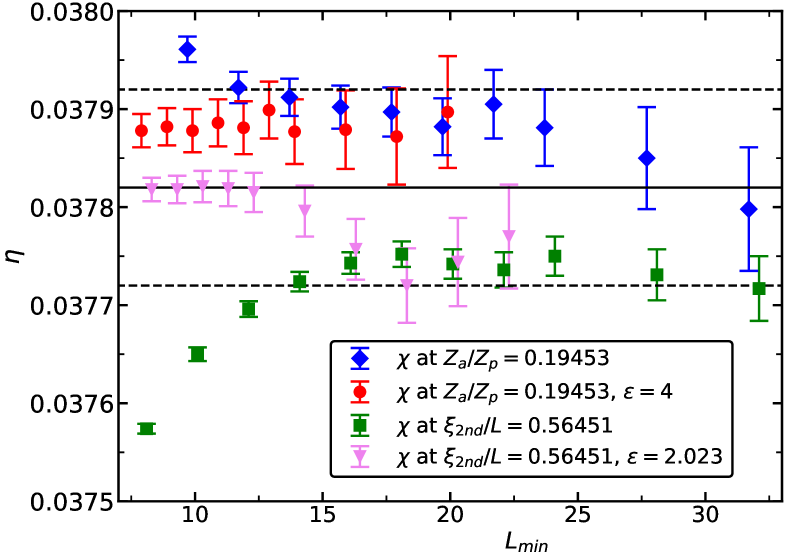
Figure 9: We give estimates of $\eta$ obtained by fitting the data for $\chi$ at $(\lambda,\mu)=(5.0,0.3)$ and $N=3$ by using the Ansätze (47,48). In the legend, for the Ansatz (48), we give the value of the correction exponent $\epsilon$. Note that the values on the $x$-axis are slightly shifted to reduce overlap of the symbols. The solid line gives our preliminary estimate of $\omega$, while the dashed lines indicate the error.

As our preliminary estimate we take $\eta=0.03782(10)$ that covers, for some range of $L_{min}$, the results obtained from all four fits.

In order to estimate the dependence of the result on $\lambda$, we analyze the data for $\lambda=4.8$ and $5.2$. Assuming that subleading corrections to scaling are very similar for these values of $\lambda$ we compare fits with small $L_{min}$, where the statistical error is small. We find, consistently for both Ansätze (47,48) and fixing $Z_{a}/Z_{p}=0.19453$ or $\xi_{2nd}=0.56451$ that the estimates of $\eta$ for $\lambda=4.8$ are larger by about $0.0001$ than for $\lambda=5.2$. In the analysis of the data for $\lambda=4.8$ and $5.2$ smaller lattices are included than for $\lambda=5.0$. Therefore the effect of corrections proportional to $L^{-\omega_{1}}$ should be smaller. Given the accuracy of $\lambda^{*}$ for the cubic fixed point we arrive at our final estimate

$$\eta=0.03782(13)\;.$$ (85)

This estimate is within the errors consistent with that obtained in Ref. myIco for the $O(3)$-invariant fixed point: $\eta_{O(3)}=0.03784(5)$. Therefore, assuming that the estimate of $\eta$ is monotonic in the scaling field of the cubic perturbation in the range that we consider here, we do not add an additional error due to the uncertainty of $\mu^{*}$.

VII.3 The critical exponent $\nu$

(Remark revised version: Also here the wrong sign of corrections in $U_{C}$ is taken. A reanalysis shows that the final result for the critical exponent $\nu$ at the cubic fixed point is uneffected.)

We have analyzed the slopes of dimensionless quantities $Z_{a}/Z_{p}-0.64U_{C}^{2}+2.1U_{C}^{3}$, $\xi_{2nd}/L+1.34U_{C}^{2}-3.4U_{C}^{3}$, and $U_{4}-1.25U_{C}^{2}-3.0U_{C}^{3}$ at $Z_{a}/Z_{p}-0.64U_{C}^{2}+2.1U_{C}^{3}=0.19477$ that stay approximately constant on the line $\lambda^{*}(\mu)$ at criticality. Below we denote these quantities by $Z_{a}/Z_{p}+...$, $\xi_{2nd}/L+...$, and $U_{4}+...$ for simplicity. We performed fits with the Ansatz (51). The resulting estimates of $y_{t}$ are plotted in Fig. 10. As our preliminary estimate we take $y_{t}=1.40635(30)$. In order to estimate the effect of corrections proportional to $L^{-\omega_{1}}$, we analyze ratios

$$r_{S,i}(L)=\frac{S_{\lambda=5.2,i}(L)}{S_{\lambda=4.8,i}(L)}\;,$$ (86)

where $i$ indicates which dimensionless quantity is taken. We expect that subleading corrections approximately cancel. Therefore we analyze these ratios with the simple Ansatz

$$r_{S,i}(L)=aL^{\Delta y_{t}}\;.$$ (87)

The estimate for $L_{min}=16$ is $\Delta y_{t}=-0.00044(10)$, $-0.00030(10)$ and $0.00021(19)$ for the slopes of $Z_{a}/Z_{p}+...$, $\xi_{2nd}/L+...$ and $U_{4}+...$, respectively. Since the difference in $\lambda$ is about 4 times as large as the uncertainty of $\lambda$ in $(\lambda,\mu)^{*}$, we conclude that the error of $y_{t}$ due to the uncertainty of $\lambda$ in $(\lambda,\mu)^{*}$ is about $0.0001$. Finally we analyzed the ratios

$$r_{S,i}(L)=\frac{S_{\mu=0.3,i}(L)}{S_{\mu=0.25,i}(L)}\;$$ (88)

for $\lambda=5.0$. Here we get $\Delta y_{t}=0.00029(9)$, $0.00019(8)$, and $0.00022(16)$ for or $Z_{a}/Z_{p}+...$, $\xi_{2nd}/L+...$ and $U_{4}+...$, respectively. Taking the estimate $\mu^{*}=0.28(2)$ we arrive at the final estimate

$$y_{t,cubic}=1.40625(50)\;,$$ (89)

which can be compared with $y_{t,O(3)}=1.4052(2)$ myIco .

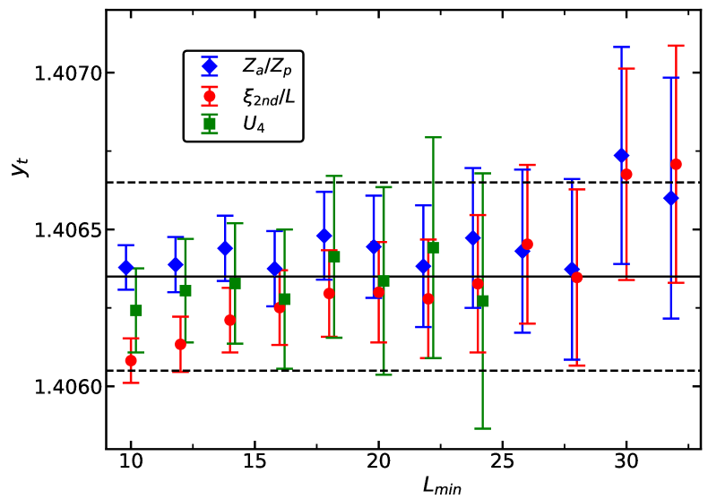
Figure 10: We give estimates of $y_{t}$ obtained by fitting the data for the slopes of $Z_{a}/Z_{p}-0.64U_{C}^{2}+2.1U_{C}^{3}$, …, at $(\lambda,\mu)=(5.0,0.3)$ and $N=3$ by using the Ansatz (51). Note that the values on the $x$-axis are slightly shifted to reduce overlap of the symbols. The solid line gives our preliminary estimate of $y_{t}$ and the dashed lines indicate the error.

VII.4 Difference between critical exponents for the $O(3)$-invariant and the cubic fixed point

(Remark revised version: Also here the wrong sign of corrections in $U_{C}$ is taken. A reanalysis shows that the final results for the critical exponents $\nu$ and $\eta$ at the cubic fixed point are uneffected. With the correct sign, the estimates of $c_{2}$ given in table 9 are consistant for the three different dimensionless quantities, with $c_{2}\approx 3.8$, while $c_{3}$ still assumes different values for different dimensionless quantities.)

Based on the expectation that corrections to scaling are similar for the improved models for the $O(3)$-invariant and the cubic fixed point, we study ratios of magnetic susceptibilities and slopes at criticality. In addition to $(\lambda,\mu)^{*}$ we analyze data for pairs $(\lambda,\mu)$ that are approximately on the line $\lambda^{*}(\mu)$. To stay critical we take the quantities at either $Z_{a}/Z_{p}-0.64U_{C}^{2}+2.1U_{C}^{3}=0.19477$ or $\xi_{2nd}/L+1.34U_{C}^{2}-3.4U_{C}^{3}=0.56404$. We evaluate ratios of slopes $S$

$$r_{S,i}(L)=\frac{S_{Cubic,i}(L)}{S_{O(3),i}(L)}\;,$$ (90)

where $i$ indicates which dimensionless quantity is taken. We analyze these ratios by fitting with the simple Ansatz

$$r_{S,i}(L)=aL^{y_{t,Cubic}-y_{t,O(3)}}$$ (91)

or as check

$$r_{S,i}(L)=aL^{y_{t,Cubic}-y_{t,O(3)}}(1+cL^{-2})\;.$$ (92)

In the case of the magnetic susceptibilities we use analogous Ansätze.

Let us first analyze the magnetic susceptibility. We only discuss $\chi$ at $\xi_{2nd}/L+1.34U_{C}^{2}-3.4U_{C}^{3}=0.56404$, since the statistical error of $\chi$ at $\xi_{2nd}/L+1.34U_{C}^{2}-3.4U_{C}^{3}=0.56404$ is clearly smaller than at $Z_{a}/Z_{p}-0.64U_{C}^{2}+2.1U_{C}^{3}=0.19477$.

For the ratio of the susceptibility at $(\lambda,\mu)=(5.0,0.3)$ and $(5.2,0)$ we get $\Delta\eta=0.00004(3)$ taking into account both the analogues of the Ansätze (91,92). As check, we computed the ratio for $(\lambda,\mu)=(5.0,0.3)$ and $(5.0,0)$. We get $\Delta\eta=0.00002(3)$.

A $\Delta\eta$ that is clearly different from zero we only get for larger values of $|\mu|$. For example for $(\lambda,\mu)=(4.7,0.7)$ and $(5.2,0)$ we get $\Delta\eta=0.00024(5)$ and for $(\lambda,\mu)=(4.8,-0.5)$ and $(\lambda,\mu)=(5.2,0)$ we get $\Delta\eta=-0.00040(5)$. We regard the estimates obtained from the susceptibility at $(\lambda,\mu)=(5.0,0.3)$ and $(5.2,0)$ or $(5.0,0)$ as bound for the difference between the cubic and the $O(3)$-invariant fixed point. Therefore

$$-0.00001\lessapprox\eta_{cubic}-\eta_{O(3)}\lessapprox 0.00007\;,$$ (93)

which is more strict than the difference of our result (85) and the estimate of $\eta_{O(3)}$ of Ref. myIco .

Finally we study ratios of slopes for $(\lambda,\mu)=(5.2,0)$ and several pairs $(\lambda,\mu)$ that approximate $\lambda^{*}(\mu)$. Our estimates are given in Fig. (11) as a function of $\bar{U}_{C}$, where $\bar{U}_{C}=[\bar{U}_{C}(L_{max})+\bar{U}_{C}(L_{min})]/2$, similar to section VII.1.3.

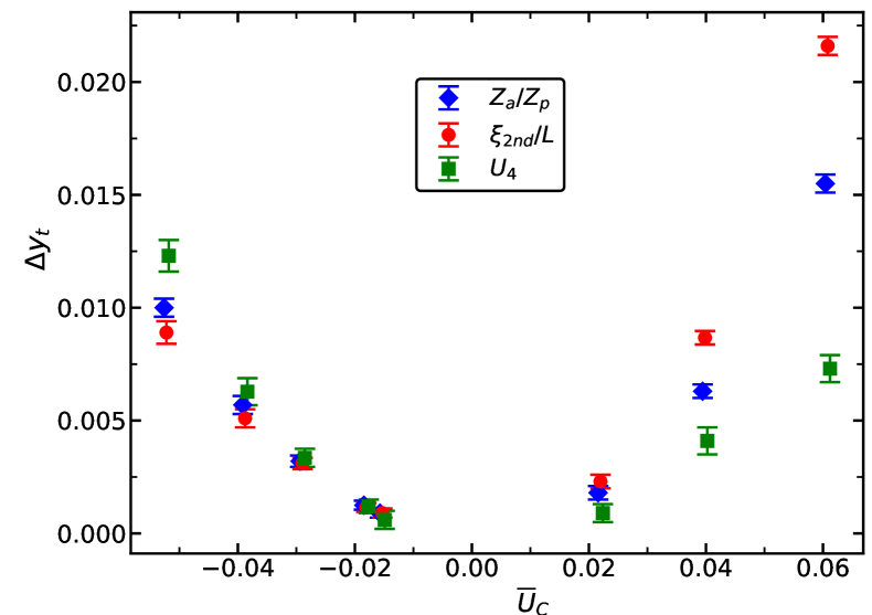
Figure 11: We plot $\Delta y_{t}$ obtained by fitting ratios of slopes for $N=3$ by using the Ansätze (91,92) as a function of $\bar{U}_{C}$. For a discussion see the text.

We have fitted the estimates with the Ansatz

$$\Delta y_{t}=c_{2}\bar{U}_{C}^{2}+c_{3}\bar{U}_{C}^{3}\;.$$ (94)

The results for the coefficients are given in table 9. Plugging in the estimate $\bar{U}_{C}^{*}=-0.0175(7)$, sec. VII.1.3, we arrive at $\Delta y_{t}=0.00117(13)$, $0.00123(13)$, and $0.00114(15)$ for $Z_{a}/Z_{p}+...$, $\xi_{2nd}/L+...$, and $U_{4}+...$, respectively. As our final estimate we quote

$$y_{t,Cubic}-y_{t,O(3)}=0.0012(2)\;,$$ (95)

where the error is dominated by the uncertainty of $U_{C}^{*}$. This result translates to

$$\nu_{Cubic}-\nu_{O(3)}=-0.00061(10)\;.$$ (96)

Table 9: Coefficients of $\Delta y_{t}=c_{2}\bar{U}_{C}^{2}+c_{3}\bar{U}_{C}^{3}$ for the slopes of three different dimensionless quantities for $N=3$. For a discussion see the text.

$R$	$c_{2}$	$c_{3}$
$Z_{a}/Z_{p}+...$	3.90(8)	4.3(1.5)
$\xi_{2nd}/L+...$	4.42(8)	23.6(1.6)
$U_{4}+...$	3.32(13)	-22.2(2.4)

VIII Comparison with results given in the literature

In the literature, information on the cubic fixed point stems mainly from field theoretic methods. The $\epsilon$-expansion has been computed up to 5-loop in Ref. Frohlinde and has recently been extended to 6-loop epsilon6 . The perturbative expansion in $d=3$ fixed has been computed up to 6-loop in Ref. Carmona . The numerical values obtained for the critical exponents vary with the resummation scheme that is used. For example, the 6-loop $\epsilon$-expansion for $N=3$ has been resummed in Ref. epsilon6 by using the Padé approximation and alternatively a by a Padé-Borel-Leroy (PBL) resummation. In Ref. AharonyNeu the resummation scheme of Ref. KoPa17 is used. For a detailed discussion of these analyses, we refer the reader to the original work.

In Ref. DBinder a large $N$-expansion around the decoupled Ising fixed point has been performed on the basis of the CB results for the Ising universality class, see Ref. Simmons-Duffin:2016wlq and references therein. The results for critical exponents obtained in Ref. DBinder are

$$\eta=0.03629+\frac{0.001232}{N}+O(N^{-2})$$ (97)

and

$$\Delta^{*}_{\epsilon}=1.5874+\frac{0.0796}{N}+O(N^{-2})\;,$$ (98)

where $\nu=1/(d-\Delta^{*}_{\epsilon})$. In tables 10 and 12 we give the numbers obtained from Eqs. (97,98) by inserting $N=3$ and $4$, respectively. Finally we give the results obtained in the present work.

Let us first discuss the numbers for $N=3$ summarized in table 10. The estimates of $\nu$ obtained from the $\epsilon$-expansion by different authors are consistent. However they are too small compared with our result. They differ from our result by more than the error that is quoted. The estimates of $\nu$ obtained from the perturbative series in $d=3$ fixed are larger than those obtained from the $\epsilon$-expansion. Still they are too small compared with ours. The estimate obtained from the large $N$-expansion is larger than ours. But one should note that the deviation is of similar size as that for the $\epsilon$-expansion, which is quite remarkable given the small value of $N$.

In the case of $\eta$ we find that the estimates obtained from the analysis of the $\epsilon$-expansion are consistent with ours, while those obtained from the perturbative series in $d=3$ fixed are smaller and the estimate of the error is smaller than the difference.

The results for the correction exponents $\omega_{1}$ and $\omega_{2}$ obtained by different authors are essentially consistent. Within errors $\omega_{1}$ of the cubic fixed point is the same as $\omega$ of the $O(3)$-invariant fixed point. For $\omega_{1}$ we have no direct numerical estimate. Our estimate of $\omega_{2}$ is larger than those obtained by field theoretic methods.

In table 11 we have selected a few results for the critical exponents for the $O(3)$-invariant fixed point. At the level of the accuracy obtained by field theoretic methods, the estimates for the critical exponents for the cubic and the $O(N)$-invariant fixed point can not be discriminated for $N=3$.

It is an interesting idea, to directly aim at the difference between the values of critical exponents for the $O(3)$-symmetric and the cubic fixed point. Given the fact that the two fixed points are close in coupling space, one might hope that systematic errors of the calculation are more or less the same and cancel when the difference is taken.

Such an analysis of the perturbative expansion in $d=3$ fixed is given in the Appendix of Ref. Calabrese . The authors find

$$\nu_{cubic}-\nu_{O(3)} = -0.0003(3)\;,$$ (99)

$$\eta_{cubic}-\eta_{O(3)} = -0.0001(1)\;,$$ (100)

$$\gamma_{cubic}-\gamma_{O(3)} = -0.0005(7)\;.$$ (101)

Our estimate $\nu_{cubic}-\nu_{O(3)}=-0.00061(10)$, Eq. (96), is consistent with that of Ref. Calabrese . In the case of $-0.00001\lessapprox\eta_{cubic}-\eta_{O(3)}\lessapprox 0.00007$, Eq. (93), we favor the opposite sign as the authors of Ref. Calabrese .

Starting from the 6-loop $\epsilon$-expansion, the authors of Ref. AharonyNeu perform an expansion of the RG-flow around the $O(3)$-symmetric fixed point to second order. Furthermore the authors have computed effective critical exponents, depending on the parameters of this RG-flow, see eqs. (14) of Ref. AharonyNeu . Plugging in the values of the parameters for the cubic fixed point, the authors get $\gamma_{cubic}=1.3849(61)$ and $\beta_{cubic}=0.3663(21)$. These values are virtually identical with $\gamma_{O(3)}=1.385(4)$ and $\beta_{O(3)}=0.3663(12)$ obtained in Ref. KoPa17 by using the same resummation scheme. Using the information given by the authors it is hard to estimate the error of the difference, which might be much smaller than the naively propagated one.

One also should note the discussion of section 5 of Ref. CB_O3 . To leading order, the deviation of the exponents of the cubic fixed point from those of the $O(3)$-invariant one is proportional to $Y_{4}$ and the coefficient is given by structure constants of the $O(3)$-invariant fixed point. For $\nu$ and $\eta$, these coefficients vanish.

There have also been attempts to isolate the cubic fixed point for $N=3$ by using the CB method Ster18 ; KoSt19 ; KoSt20 . However the candidate that is found, has critical exponents and a correction exponent very different from those discussed here.

Table 10: Estimates of the exponents $\nu$, $\eta$, and $\gamma$ and the correction exponents $\omega_{1}$ and $\omega_{2}$ for the cubic fixed point for $d=3$ and $N=3$. Aharony et al. AharonyNeu only quote the result for the exponents $\beta$ and $\gamma$ (see their table II). They give $\beta=0.3669(12)$. Inserting our results for $\nu$ and $\eta$, we arrive at $\beta=\frac{\nu}{2}(d-2+\eta)=0.3690(2)$. ^∗ indicates that the Monte Carlo result for $\gamma$ is obtained by inserting our numerical estimates of $\nu$ and $\eta$ into $\gamma=\nu(2-\eta)$. For a discussion see the text.

Ref.	method	$\omega_{1}$	$\omega_{2}$	$\nu$	$\eta$	$\gamma$
Mud98	5-loop $\epsilon$-exp			0.6997(24)	0.0375(5)	1.3746(20)
Carmona	5-loop $\epsilon$-exp	0.799(14)	0.006(4)	0.701(4)	0.0374(22)	1.377(6)
Carmona	6-loop $d=3$ fix	0.781(4)	0.010(4)	0.706(6)	0.0333(26)	1.390(12)
Varna00	6-loop $d=3$ fix	0.7833(54)	0.0109(32)	0.7040(40)	0.0327(20)	1.3850(50)
Folk00	6-loop $d=3$ fix	0.777(9)		0.705(1)		1.387(1)
epsilon6	6-loop $\epsilon$-exp, PBL	0.799(4)	0.005(5)	0.700(8)	0.036(3)	1.368(12)
epsilon6	6-loop $\epsilon$-exp, Padé	0.78(11)	0.008(38)	0.703(5)	0.038(4)	1.379(8)
AharonyNeu	6-loop $\epsilon$-exp					1.387(9)
DBinder	Large $N$			0.7215	0.03671
this work	MC		0.0133(8)	0.7111(3)	0.03782(13)	1.3953(6)∗

Table 11: Estimates of the exponents $\nu$, $\eta$, $\gamma$, and $Y_{4}$ and the correction exponent $\omega$ for the Heisenberg fixed point for $d=3$ and $N=3$. ^∗ indicates that in the case of Ref. myIco , we computed $\gamma=(2-\eta)\nu$ by using the values given for $\nu$ and $\eta$. For a discussion see the text.

Ref.	method	$\omega$	$Y_{4}$	$\nu$	$\eta$	$\gamma$
GuZi98	5-loop $\epsilon$-exp	0.794(18)		0.7045(55)	0.0375(45)	1.3820(90)
GuZi98	$d=3$	0.782(13)		0.7073(35)	0.0355(25)	1.3895(50)
KoPa17	6-loop $\epsilon$-exp	0.795(7)		0.7059(20)	0.0378(5)
Carmona	5-loop $\epsilon$-exp		0.003(4)
Carmona	6-loop $d=3$		0.013(6)
AharonyNeu	6-loop $\epsilon$-exp	0.7967(57)	0.0083(15)
CB_O3	CB		$>$0.00944	0.71169(30)	0.037884(102)
O234	MC		0.013(4)
myIco	MC	0.759(2)		0.71164(10)	0.03784(5)	1.39635(20)∗
this work	MC, Sec. VI		0.0143(9)
this work	MC, Sec. VII.1.3		0.0142(6)

Table 12: Estimates of the exponents $\nu$, $\eta$, and $\gamma$ and the correction exponents $\omega_{1}$ and $\omega_{2}$ for the cubic fixed point for $d=3$ and $N=4$. ^∗ indicates that the Monte Carlo result for $\gamma$ is obtained by inserting our numerical estimates of $\nu$ and $\eta$ into $\gamma=\nu(2-\eta)$. For a discussion see the text.

Ref.	method	$\omega_{1}$	$\omega_{2}$	$\nu$	$\eta$	$\gamma$
Mud98	5-loop $\epsilon$-exp			0.7225(22)	0.0365(5)	1.4208(30)
Carmona	5-loop $\epsilon$-exp	0.790(8)	0.078(4)	0.723(4)	0.0357(18)	1.419(6)
Carmona	6-loop $d=3$ fix	0.781(44)	0.076(40)	0.714(8)	0.0316(22)	1.405(10)
Varna00	6-loop $d=3$ fix	0.7887(90)	0.0740(65)	0.7150(50)	0.0316(25)	1.4074(30)
Folk00	6-loop $d=3$ fix	0.777(2)		0.719(2)		1.416(4)
DBinder	Large $N$			0.7180	0.03661
this work	MC	0.763(24)	0.082(5)	0.7202(7)	0.0371(2)	1.4137(14)∗

Let us discuss the results for $N=4$ summarized in table 12. Here we see that the estimates of $\nu$ obtained by the various authors are consistent with our result. The estimate obtained by the large $N$-expansion is slightly smaller than ours. Note that for $N=3$ it is bigger and the deviation is roughly by a factor of 4 larger than for $N=4$. It is plausible that for $N\geq 5$ the large $N$-expansion expansion gives very accurate results and might serve as benchmark for the analysis of the $\epsilon$-expansion or the perturbative expansion in $d=3$ fixed. In the case of the exponent $\eta$ the findings are similar to $N=3$. The results obtained from the $\epsilon$-expansion are consistent with ours, while those obtained from the perturbative expansion in $d=3$ fixed are too small. The estimate obtained from the large $N$-expansion is slightly smaller than ours. The deviation is much smaller than for $N=3$. It is plausible that for $N\geq 5$ the deviation of the large $N$-expansion from the exact value is at most in the $5^{th}$ digit.

The estimates of $\omega_{2}$ are consistent among different authors and the field theoretic results are consistent with that obtained here. Our estimate of $\omega_{1}$ is smaller than that obtained by field theoretic methods, which also holds in the case of $\omega$ for the $O(4)$-symmetric fixed point myON . Within error bars our estimate of $\omega_{1}$ takes the same value as $\omega$ for the $O(4)$-symmetric fixed point myON .

In contrast to $N=3$, truncating the expansion of the scaling fields of the $O(N)$-invariant fixed point at second order is no good approximation. This is seen for example by the fact that $Y_{4}$ and $\omega_{2}$ clearly differ.

IX Summary and Conclusions

We have studied a $\phi^{4}$ model on the simple cubic lattice, where the reduced Hamiltonian, Eq. (4), includes a term that breaks $O(N)$ invariance and possesses only cubic symmetry. It has two parameters $\lambda$ and $\mu$, where $\mu$ controls the breaking of the $O(N)$ invariance. Field theory predicts that for $N>N_{c}$ the perturbation of the $O(N)$-invariant fixed point is relevant, where $N_{c}$ is slightly smaller than three. In fact the recent conformal bootstrap study CB_O3 finds the rigorous bound $Y_{4}>3-2.99056$ for the RG-exponent of a cubic perturbation for $N=3$. Depending on the sign of the parameter $\mu$, the system should undergo a first order phase transition or a continuous transition governed by the cubic fixed point. For a recent discussion of the implications for structural transition in perovskites see Ref. AharonyNeu .

For $N=4$ the cubic fixed point is well separated from the $O(4)$-symmetric one. Using a finite size scaling analysis of dimensionless quantities such as the Binder cumulant $U_{4}$, we determine the improved model, characterized by $(\lambda,\mu)^{*}$, where the two leading corrections to scaling vanish. In order to monitor the violation of the $O(N)$ symmetry the cumulant $U_{C}$, Eq. (15), is introduced. It vanishes for an $O(N)$-symmetric distribution of the order parameter. At $(\lambda,\mu)^{*}$, we determine the critical exponents $\nu$ and $\eta$ by using standard finite size scaling methods. For $N=4$ these are clearly different from those of $O(4)$-symmetric systems. For the correction exponents we obtain $\omega_{1}=0.763(24)$ and $\omega_{2}=0.082(5)$ for $N=4$. One should note that in order to reduce the effect of corrections proportional to $L^{-\omega_{2}}$ for example by half, one has to increase the linear lattice size by the factor $2^{1/\omega_{2}}\approx 4700$. It is clear that in a Monte Carlo study of lattice models, we can not approach the cubic fixed point by just increasing the linear lattice size $L$. It is mandatory to eliminate corrections proportional to $L^{-\omega_{2}}$ by a proper choice of the parameters! This is even more the case for $N=3$, where we find $\omega_{2}=0.0133(8)$.

In the experimentally relevant case $N=3$, the cubic fixed point is close to the $O(3)$-invariant one. This is related to the fact that the correction and RG exponents $\omega_{2}\approx Y_{4}=0.0143(9)$ have a small modulus. This also implies that there is a slow RG-flow along a line in coupling space. In order to analyze the behavior of dimensionless quantities we use Ansätze that are approximately valid in a region of the parameter space that includes both the $O(3)$-symmetric and the cubic improved models. This allows us to determine a line $\lambda^{*}(\mu)$ in the $(\lambda,\mu)$ plane, onto which the RG-flow rapidly collapses.

In order to study the flow of the symmetry breaking perturbation, we focus on the dimensionless quantity $U_{C}$. Based on the RG-flow equation to second order, Eq. (37), we obtain an Ansatz for $U_{C}$ that is a good approximation in a region of the parameter space that includes both improved models. We obtain the estimate $(\lambda,\mu)^{*}=(4.99(11),0.28(2))$, characterizing the improved model for the cubic fixed point. Estimates of the exponents $\nu$ and $\eta$ of the cubic fixed point are obtained by analyzing the slopes of dimensionless quantities and the magnetic susceptibility at $(\lambda,\mu)=(5.0,0.3)$ and values close by. It turns out that the estimate of $\eta$ is the same as that for the $O(3)$-symmetric fixed point within errors. In the case of the exponent of the correlation length the estimate $\nu_{cubic}=0.7111(3)$ obtained for the cubic fixed point is only slightly smaller than that for the $O(3)$-symmetric one $\nu_{O(3)}=0.71164(10)$ myIco . Since we have estimated the error conservatively here, we consider the difference as significant.

In Sec. VII.1.3 we go beyond the second order approximation of the RG-flow. In the second order approximation $Y_{4}=\omega_{2}$, while in Sec. VII.1.3 we find $0\lessapprox Y_{4}-\omega_{2}\lessapprox 0.0015$.

In Sec. (VII.4) we analyze ratios of magnetic susceptibilities and slopes of dimensionless quantities to get estimates of the differences of the critical exponents for the cubic and the $O(3)$-invariant fixed point. The idea is that subleading corrections approximately cancel, and the systematic error is reduced in the difference. In fact, we arrive at $-0.00001\lessapprox\eta_{cubic}-\eta_{O(3)}\lessapprox 0.00007$ and $\nu_{Cubic}-\nu_{O(3)}=-0.00061(10)$.

The results of the present work can be improved by simply increasing the statistics and moderately increasing the linear lattices sizes. Beyond that we would like to extend the study for $N=3$ in the following directions:

• Study $|\mu|>1$. In particular we would like to extend the flow equation for $\bar{U}_{C}$ discussed in Sec. VII.1.3 to larger values of $|\bar{U}_{C}|$. On the one hand we like to extend the range up to the decoupled Ising fixed point and on the other hand we like to see clear signs of the first order transition in the simulation.

• Here we studied finite systems at criticality. It would be interesting to study the case $\xi\ll L$ that approximates the thermodynamic limit in the phases. One could compute universal amplitude ratios that can be compared with results obtained in experiments.

• Extending the calculation of RG-exponents to a larger set of operators. In section 5 of Ref. CB_O3 it is discussed that for example the RG-exponent of the rank-2 symmetric tensor should have a contribution at leading order in $Y_{4}$, in contrast to the singlet and vector operators studied here.

X Acknowledgement

This work was supported by the Deutsche Forschungsgemeinschaft (DFG) under the grant HA 3150/5-3.

References

- (1) A. Pelissetto and E. Vicari, Critical Phenomena and Renormalization-Group Theory, [arXiv:cond-mat/0012164], Phys. Rept. 368, 549 (2002).
- (2) M. Campostrini, M. Hasenbusch, and A. Pelissetto, P. Rossi, and E. Vicari, Critical Exponents and Equation of State of the Three-Dimensional Heisenberg Universality Class, [arXiv:cond-mat/0110336], Phys. Rev. B 65, 144520 (2002).
- (3) K. G. Wilson and M. E. Fisher, Critical Exponents in 3.99 Dimensions, Phys. Rev. Lett. 28, 240 (1972).
- (4) A. Aharony, Critical Behavior of Anisotropic Cubic Systems, Phys. Rev. B 8, 4270 (1973).
- (5) A. Aharony, Critical Behavior of Anisotropic Cubic Systems in the Limit of Infinite Spin Dimensionality, Phys. Rev. Lett. 31, 1494 (1973).
- (6) Damon J. Binder, The Cubic Fixed Point at Large , [arXiv:2106.03493], JHEP 09 (2021) 079.
- (7) J. M. Carmona, A. Pelissetto, and E. Vicari, The -component Ginzburg-Landau Hamiltonian with cubic anisotropy: A Six loop study, [arXiv:cond-mat/9912115], Phys. Rev. B 61, 15136 (2000).
- (8) K. B. Varnashev, Stability of a cubic fixed point in three-dimensions: Critical exponents for generic , [arXiv:cond-mat/9909087], Phys. Rev. B 61, 14660 (2000).
- (9) R. Folk, Y. Holovatch and T. Yavors’kii, Pseudo-expansion of six-loop renormalization-group functions of an anisotropic cubic model, [arXiv:cond-mat/0003216], Phys. Rev. B 62, 12195 (2000).
- (10) H. Kleinert and V. Schulte-Frohlinde, Exact Five-Loop Renormalization Group Functions of -Theory with -Symmetric and Cubic Interactions. Critical Exponents up to , [arXiv:cond-mat/9503038], Phys. Lett. B 342, 284 (1995).
- (11) John Cardy, Scaling and Renormalization in Statistical Physics, Series: Cambridge Lecture Notes in Physics (No. 5) (Cambridge University Press, Cambridge, 1996)
- (12) Loran Ts. Adzhemyan, Ella V. Ivanova, Mikhail V.Kompaniets, Andrey Kudlis, and Aleksandr I. Sokolov, Six-loop -expansion study of three-dimensional -vector model with cubic anisotropy, [arXiv:1901.02754], Nucl. Phys. B 940, 332 (2019).
- (13) A. Aharony, O. Entin-Wohlman and A. Kudlis, Different critical behaviors in cubic to trigonal and tetragonal perovskites, [arXiv:2201.08252], Phys. Rev. B 105, 104101 (2022).
- (14) M. Hasenbusch and E. Vicari, Anisotropic perturbations in three-dimensional O(N)-symmetric vector models, [arXiv:1108.0491], Phys. Rev. B 84, 125136 (2011).
- (15) Shai M. Chester, Walter Landry, Junyu Liu, David Poland, David Simmons-Duffin, Ning Su, and Alessandro Vichi, Bootstrapping Heisenberg Magnets and their Cubic Instability, [arXiv:2011.14647], Phys. Rev. D 104, 105013 (2021).
- (16) M. Hasenbusch, Monte Carlo study of a generalized icosahedral model on the simple cubic lattice, [arXiv:2005.04448], Phys. Rev. B 102, 024406 (2020).
- (17) J. H. Chen, M. E. Fisher and B. G. Nickel, Unbiased Estimation of Corrections to Scaling by Partial Differential Approximants, Phys. Rev. Lett. 48, 630 (1982).
- (18) M. E. Fisher and J. H. Chen, The validity of hyperscaling in three dimensions for scalar spin systems, J. Physique (Paris) 46, 1645 (1985).
- (19) M. N. Barber, Finite-size Scaling in Phase Transitions and Critical Phenomena, Vol. 8, eds. C. Domb and J. L. Lebowitz, (Academic Press, 1983)
- (20) H. W. J. Blöte, E. Luijten and J. R. Heringa, Ising universality in three dimensions: a Monte Carlo study, [arXiv:cond-mat/9509016], J. Phys. A: Math. Gen. 28, 6289 (1995).
- (21) H. G. Ballesteros, L. A. Fernández, V. Martín-Mayor, and A. Muñoz Sudupe, Finite Size Scaling and “perfect” actions: the three dimensional Ising model, [arXiv:hep-lat/9805022], Phys. Lett. B 441, 330 (1998).
- (22) M. Hasenbusch, K. Pinn, and S. Vinti, Critical Exponents of the 3D Ising Universality Class From Finite Size Scaling With Standard and Improved Actions, [arXiv:hep-lat/9806012], Phys. Rev. B 59, 11471 (1999).
- (23) M. Hasenbusch, A Monte Carlo study of leading order scaling corrections of theory on a three dimensional lattice, [hep-lat/9902026], J. Phys. A 32, 4851 (1999).
- (24) M. Hasenbusch, Eliminating leading corrections to scaling in the 3-dimensional O(N)-symmetric model: and , [arXiv:cond-mat/0010463], J. Phys. A 34, 8221 (2001).
- (25) M. Campostrini, M. Hasenbusch, A. Pelissetto, P. Rossi, and E. Vicari, Critical behavior of the three-dimensional XY universality class, [arXiv:cond-mat/0010360], Phys. Rev. B 63, 214503 (2001).
- (26) M. Hasenbusch, Restoring isotropy in a three-dimensional lattice model: The Ising universality class, [arXiv:2105.09781], Phys. Rev. B 104, 014426 (2021).
- (27) Martin Hasenbusch, Three-dimensional -invariant models at criticality for , [arXiv:2112.03783], Phys. Rev. B 105, 054428 (2022).
- (28) U. Wolff, Collective Monte Carlo Updating for Spin Systems, Phys. Rev. Lett. 62, 361 (1989).
- (29) Martin Hasenbusch, Dynamic critical exponent z of the three-dimensional Ising universality class: Monte Carlo simulations of the improved Blume-Capel model, [arXiv:1908.01702], Phys. Rev. E 101, 022126 (2020).
- (30) Eduardo Fradkin, Quantum Field Theories, An Integrated Approach, Princton University Press, Princton and Oxford, (2021).
- (31) D. Banerjee, S. Chandrasekharan, and D. Orlando, Conformal dimensions via large charge expansion, [arXiv:1707.00711], Phys. Rev. Lett. 120, 061603 (2018).
- (32) D. Banerjee, S. Chandrasekharan, D. Orlando, and S. Reffert, Conformal Dimensions in the Large Charge Sectors at the Wilson-Fisher Fixed Point, [arXiv:1902.09542], Phys. Rev. Lett. 123, 051603 (2019).
- (33) M. V. Kompaniets and E. Panzer, Minimally subtracted six-loop renormalization of -symmetric theory and critical exponents, [arXiv:1705.06483], Phys. Rev. D 96, 036016 (2017).
- (34) D. Simmons-Duffin, The Lightcone Bootstrap and the Spectrum of the 3d Ising CFT, [arXiv:1612.08471], JHEP 03 (2017) 086.
- (35) P. Calabrese, A. Pelissetto and E. Vicari, Randomly dilute spin models with cubic symmetry, [arXiv:cond-mat/0202292], Phys. Rev. B 67, 024418 (2003).
- (36) Andreas Stergiou, Bootstrapping hypercubic and hypertetrahedral theories in three dimensions, [arXiv:1801.07127], JHEP 05 (2018) 035.
- (37) Stefanos R. Kousvos and Andreas Stergiou, Bootstrapping mixed correlators in three-dimensional cubic theories, [arXiv:1810.10015], SciPost Phys. 6, 035 (2019).
- (38) Stefanos R. Kousvos and Andreas Stergiou, Bootstrapping mixed correlators in three-dimensional cubic theories II, [arXiv:1911.00522], SciPost Phys. 8, 085 (2020).
- (39) A. I. Mudrov and K. B. Varnashev, Modified Borel summation of divergent series and critical-exponent estimates for an -vector cubic model in three dimensions from five-loop expansions, [arXiv:cond-mat/9805081], Phys. Rev. E 58 5371, (1998).
- (40) R. Guida and J. Zinn-Justin, Critical exponents of the N vector model, [arXiv:cond-mat/9803240], J. Phys. A 31, 8103 (1998).