Robust boundary integral equations for the solution of elastic scattering problems via Helmholtz decompositions

Abstract

Helmholtz decompositions of the elastic fields open up new avenues for the solution of linear elastic scattering problems via boundary integral equations (BIE) [19]. The main appeal of this approach is that the ensuing systems of BIE feature only integral operators associated with the Helmholtz equation. However, these BIE involve non standard boundary integral operators that do not result after the application of either the Dirichlet or the Neumann trace to Helmholtz single and double layer potentials. Rather, the Helmholtz decomposition approach leads to BIE formulations of elastic scattering problems with Neumann boundary conditions that involve boundary traces of the Hessians of Helmholtz layer potential. As a consequence, the classical combined field approach applied in the framework of the Helmholtz decompositions leads to BIE formulations which, although robust, are not of the second kind. Following the regularizing methodology introduced in [3] we design and analyze novel robust Helmholtz decomposition BIE for the solution of elastic scattering that are of the second kind in the case of smooth scatterers in two dimensions. We present a variety of numerical results based on Nyström discretizations that illustrate the good performance of the second kind regularized formulations in connections to iterative solvers.
Keywords: Time-harmonic Navier scattering problems, Helmholtz decomposition, boundary integral equations, pseudodifferential calculus, Nyström discretizations, preconditioners.

AMS subject classifications: 65N38, 35J05, 65T40, 65F08

1 Introduction

The extension of Boundary Integral Equation (BIE) based discretizations for the numerical solution of acoustic scattering problems (i.e. Helmholtz equations) to their elastic scattering problems (i.e. Navier equations) counterpart is thought to be more or less straightforward. Typically, BIE for elastic scattering problems are based on the Navier Green’s function, which albeit more complicated than the Helmholtz Green’s function (not in the least because it involves two wave-numbers), exhibits the same singularity type as the latter. Therefore, discretization methods that rely on kernel independent quadratures, that is these quadratures resolve in a black box manner the singularities of Green’s functions together with their derivatives, can be extended from the Helmholtz to the Navier case without much fuss. Amongst these types of discretizations we mention the $\delta$-BEM methods [14, 12, 13, 15] and the Density Interpolation Methods [21]. On the other hand, other discretizations strategy such as the Kussmaul-Martensen singularity splitting Nyström methods can be extended from the Helmholtz to the Navier setting but require cumbersome modifications [10, 17].

Recently a new BIE approach to elastic scattering problems shortcuts the need to use Navier Green’s functions and relies entirely on Helmholtz layer potentials [19, 28]. This approach is based on Helmholtz decompositions of elastic waves into compressional and shear waves, a manner which reduces the elastic scattering problem, at least in two dimensions, to the solution of two Helmholtz equations coupled by their boundary values on the scatterers. In three dimensions this approach leads to coupling the solution of a Helmholtz scattering problem to that of a Maxwell scattering problem [20]. These recent contributions consider only single layer potential representations of Helmholtz fields and elastodynamic fields with Dirichlet boundary conditions on the boundary of the scatterers, and, therefore, the ensuing BIE are not robust for all frequencies. We extended the Helmholtz decomposition approach in two dimensions to Neumann boundary conditions as well as for combined field representations in [18]. The extension of the Helmholtz decomposition approach to the Neumann case is nontrivial since it gives rise to non standard Boundary Integral Operators (BIOs) which arise from applications of boundary traces to Hessians of single and double layer Helmholtz potentials. More importantly, the BIE Helmholtz decomposition route is a viable approach to the solution of elastic scattering problems in as much as robust formulations are used. The goal of this paper is to derive and analyze such robust formulations, including some which are of the second kind in the case of smooth scatterers.

The most widely used strategy to deliver robust BIE formulations for the solution of time harmonic scattering problems is the combined field (CFIE) strategy [4, 6]. The analysis of such formulations relies on the Fredholm theory and the well posedness of Robin boundary value problems in bounded/interior domains. The analysis of the Fredholm property of the BIOs that arise in the combined field strategy in the Helmholtz decomposition framework for elastic scattering problems is a bit more delicate, as it requires the use of lower order terms in the asymptotic expansion in the pseudodifferential sense of the constitutive BIOs. The reason for this more involved analysis is the fact that the principal symbols of these operators (unlike the Helmholtz case) are defective, which was already remarked in [19]. However, the ensuing CFIE feature pseudodifferential operators of order one (Dirichlet) and respectively two (Neumann) and a such are not ideal for iterative solutions.

In order to design integral formulations of the second kind for the solution of elastic scattering problems via the Helmholtz decomposition approach we employ the general methodology in [3]. Using coercive approximations of Dirichlet to Neumann (DtN) operators, we construct certain regularizing operators that are approximations of the operators that map the boundary conditions in the Helmholtz decomposition approach to the Helmholtz Cauchy data on the boundary of the scatterer. The regularizing operators we consider, whose construction relies on the pseudodifferential calculus, are based on either square root Fourier multipliers or Helmholtz BIOs, and are straightforward to implement in existing discretizations methodologies for Helmholtz BIOs. More importantly, we prove that in the case of smooth scatterers the regularized formulations are robust and of the second kind, and we provide numerical evidence about the superior performance of these formulations over the combined field formulations with respect to iterative solvers. Thus, we show in this paper that it is possible to construct BIE with good spectral properties for the solution of the elastic scattering problems in two dimensions via Helmholtz decompositions, making this approach a viable alternative to the recently introduced BIE based on the Navier Green’s function [8, 9, 17, 5]. The extension of this approach to three dimensional elastic scattering problem is currently ongoing.

The paper is organized as follows: in Section 2 we introduce the Navier equations in two dimensions and we present the Helmholtz decomposition approach; in Section 3 we present the trace for the gradient and Hessian of the boundary layer operators for Helmholtz equation. We also review certain properties of Helmholtz BIOs with asymptotic expansions of in the pseudodifferential sense. The proof of these result is postponed to the self-contained Appendix and presented here just for the sake of completeness; in Section 4 we analyze the nonstandard BIOs that arise in the Helmholtz decomposition approach for Dirichlet (subsection 4.1) and Neumann (subsection 4.2) boundary conditions. Finally, we present in Section 5 a variety of numerical results illustrating the iterative behavior of solvers based on Nyström discretizations of the various BIE formulations of the Helmholtz decomposition approach in the high frequency regime.

2 Navier equations

For any vector function ${\bf u}=(u_{1},u_{2})^{\top}:\mathbb{R}^{2}\to\mathbb{R}^{2}$ (vectors in this paper will be always regarded as column vectors) the strain tensor in a linear isotropic and homogeneous elastic medium with Lamé constants $\lambda$ and $\mu$ is defined as

$$\bm{\epsilon}({\bf u}):=\frac{1}{2}(\nabla{\bf u}+(\nabla{\bf u})^{\top})=\begin{bmatrix}\partial_{x_{1}}u_{1}&\tfrac{1}{2}\left(\partial_{x_{1}}u_{2}+\partial_{x_{2}}u_{1}\right)\\ \tfrac{1}{2}\left(\partial_{x_{1}}u_{2}+\partial_{x_{2}}u_{1}\right)&\partial_{x_{2}}u_{2}\end{bmatrix}.$$

The stress tensor is then given by

$$\bm{\sigma}({\bf u}):=2\mu\bm{\epsilon}({\bf u})+\lambda(\operatorname{div}{\bf u})I_{2}$$

where $I_{2}$ is the identity matrix of order 2 and the Lamé coefficients $\lambda$ are assumed to satisfy $\lambda,\ \lambda+2\mu>0$. The time-harmonic elastic wave (Navier) equation is

$$\operatorname{div}\bm{\sigma}({\bf u})+\omega^{2}{\bf u}=\mu\Delta{\bf u}+(\lambda+\mu)\nabla(\operatorname{div}{\bf u})+\omega^{2}{\bf u}=0$$

where the frequency $\omega\in\mathbb{R}^{+}$ and the divergence operator ${\rm div}$ is applied row-wise.

Considering a bounded domain $\Omega$ in $\mathbb{R}^{2}$ whose boundary $\Gamma$ is a closed smooth curve, we are interested in solving the impenetrable elastic scattering problem in the exterior of $\Omega$, denoted from now on as $\Omega^{+}$. That is, we look for solutions of the time-harmonic Navier equation

$$\operatorname{div}\bm{\sigma}({\bf u})+\omega^{2}{\bf u}=0\quad{\rm in}\ \mathbb{R}^{2}\setminus\Omega$$ (2.1)

that satisfy the Kupradze radiation condition at infinity [1, 27]: if

$$\mathbf{u}_{p}:=-\frac{1}{k_{p}^{2}}\nabla\operatorname{div}\mathbf{u},\quad\mathbf{u}_{s}:=\mathbf{u}-\mathbf{u}_{p}=\operatorname{\overrightarrow{\mathrm{curl}}}{\rm{curl}\ {\bf u}}$$ (2.2)

($\operatorname{\overrightarrow{\mathrm{curl}}}\varphi:=(\partial_{x_{2}}\varphi,-\partial_{x_{1}}\varphi)$, $\operatorname{curl}{\bf u}:=\partial_{x_{2}}u_{1}-\partial_{x_{1}}u_{2}$ are respectively the vector and scalar curl, or rotational, operator) with

$$k_{p}^{2}:=\frac{\omega^{2}}{\lambda+2\mu},\quad k_{s}^{2}:=\frac{\omega^{2}}{\mu}$$ (2.3)

the associated the pressure and stress wave-numbers wave-numbers, then

$$\frac{\partial\mathbf{u}_{p}}{\partial\widehat{\bm{x}}}(\bm{x})-ik_{p}\mathbf{u}_{p}(\bm{x}),\quad\frac{\partial\mathbf{u}_{s}}{\partial\widehat{\bm{x}}}(\bm{x})-ik_{s}\mathbf{u}_{s}(\bm{x})=o\left(|\bm{x}|^{-1/2}\right),\quad\widehat{\bm{x}}:=\frac{1}{|\bm{x}|}\bm{x}.$$

On the boundary $\Gamma$ the solution ${\bf u}$ of (2.1) satisfies either the Dirichlet boundary condition

$${\bf u}={\bf f}\quad{\rm on}\ \Gamma$$

or the Neumann boundary condition

$$T{\bf u}:=\bm{\sigma}({\bf u})\bm{n}=\lambda\operatorname{div}{\bf u}-2\mu(\nabla{\bf u})\bm{t}={\bf g}\quad{\rm on}\ \Gamma.$$

Here $\bm{n}$ is unit normal vector pointing outward and

$$\bm{t}:=-\mathrm{Q}\bm{n},\quad\mathrm{Q}:=\begin{bmatrix}&1\\ -1&\end{bmatrix}$$

the unit tangent field positively (counterclockwise if $\Gamma$ is simply connected) oriented.

In view of (2.2) we can look for the fields ${\bf u}$ in the form

$${\bf u}=\nabla u_{p}+\operatorname{\overrightarrow{\mathrm{curl}}}{u_{s}}$$ (2.4)

where $u_{p}$ and $u_{s}$ are respectively solutions of the Helmholtz equations in $\Omega^{+}$ with wave-numbers $k_{p}$ and $k_{s}$ fulfilling the radioactive, or Sommerfeld, condition at infinity (as consequence of the Kupradze radiation condition) .

In the case of Dirichlet boundary conditions, by taking the scalar product of the decomposition (2.4) with the orthogonal frame $(\bm{t},\bm{n})$ on $\Gamma$, it is straightforward to see that $u_{p}$ and $u_{s}$ must satisfy the following coupled boundary conditions

$$\left|\begin{array}[]{rcll}\partial_{\bm{n}}u_{p}+\partial_{\bm{t}}u_{s}&=&-{\bf u}^{\rm inc}\cdot\bm{n},&{\rm on}\ \Gamma\\ \partial_{\bm{t}}u_{p}-\partial_{\bm{n}}u_{s}&=&-{\bf u}^{\rm inc}\cdot\bm{t},&{\rm on}\ \Gamma.\end{array}\right.$$ (2.5)

In the case of Neumann boundary conditions, the same approach described above combined with the identities

$$T[\nabla u_{p}] = 2\mu\operatorname{Hes}u_{p}+\lambda\Delta u_{p}=2\mu\operatorname{Hes}u_{p}-\lambda k_{p}^{2}u_{p}$$

$$T[\overrightarrow{{\rm curl}}_{p}u_{s}] = {\rm Q}(2\mu\operatorname{Hes}u_{s}-\mu\Delta u_{s})={\rm Q}(2\mu\operatorname{Hes}u_{s}+\mu k^{2}_{s}u_{s})$$

where $\operatorname{Hes}:=\nabla\nabla^{\top}$ is the Hessian matrix operator, imply that $u_{p}$ and $u_{s}$ must satisfy the following coupled boundary conditions

$$\left|\begin{array}[]{rclrcl}2\mu\bm{n}^{\top}\operatorname{Hes}u_{p}{\bm{n}}-\lambda k_{p}^{2}u_{p}&+&2\mu\bm{t}^{\top}\operatorname{Hes}u_{s}{\bm{n}}&=&-T{\bf u}^{\rm inc}\cdot{\bm{n}},&{\rm on}\ \Gamma\\ 2\mu\bm{t}^{\top}\operatorname{Hes}u_{p}{\bm{n}}&-&2\mu\bm{n}^{\top}\operatorname{Hes}u_{s}{\bm{n}}-\mu k_{s}^{2}u_{s}&=&-T{\bf u}^{\rm inc}\cdot{\bm{t}},&{\rm on}\ \Gamma.\\ \end{array}\right.$$ (2.6)

The goal of this paper is to develop robust BIE formulations for the solution of elastic scattering problems based on the Helmholtz decomposition approach in connection with the systems of boundary conditions (2.5) and respectively (2.6). The BIE we develop use Helmholtz potentials, for which reason we review certain properties of those next section.

Remark 2.1

Throughout this article, except in the Appendix, we will assume that $\Gamma$ is of length $2\pi$. This simplifies some of the following expressions. The modifications needed to cover the case of arbitrary length curves essentially consist of replacing the wave-number(s) $k$ (as well as $k_{p}$, $k_{s}$ and its complexifications $\widetilde{k}_{p}$ and $\widetilde{k}_{s}$) by $Lk/(2\pi)$, its characteristic length. We can see this either by adapting the analysis or by a simple scaling argument.

3 Helmholtz BIOs, gradient and Hessian calculations

For a given wave-number $k$ and a functional density $\varphi$ on the boundary $\Gamma$ we define the Helmholtz single and double layer potentials in the form

$$\operatorname{SL}_{k}[\varphi]({\bm{x}}):=\int_{\Gamma}\phi_{k}({\bm{x}}-{\bm{y}})\varphi({\bm{y}}){{\rm d}{\bm{y}}},\quad\operatorname{DL}_{k}[\varphi]({\bm{x}}):=\int_{\Gamma}\frac{\partial\phi_{k}({\bm{x}}-{\bm{y}})}{\partial\bm{n}({\bm{y}})}\varphi({\bm{y}}){{\rm d}{\bm{y}}},\ {\bm{x}}\in\mathbb{R}^{2}\setminus\Gamma.$$

where $k>0$ and

$$\phi_{k}({\bm{x}})=\frac{i}{4}H_{0}^{(1)}(k|{\bm{x}}|)$$

is the fundamental solution of the Helmholtz equation.

The four BIOs of the Calderón’s calculus associated with the Helmholtz equation are defined by applying the exterior/interior Dirichlet and Neumann traces on $\Gamma$ (denoted in what follows by $\gamma^{+}/\gamma^{-}$ and $\partial_{\bm{n}}^{+}/\partial_{\bm{n}}^{-}$ respectively) to the Helmholtz single and double layer potentials defined above via the classical relations [22, 29, 31]

$$\gamma^{\pm}\operatorname{SL}_{k}\varphi =\operatorname{V}_{k}\varphi,\quad \partial_{\bm{n}}^{\pm}\operatorname{SL}_{k}\varphi =\mp\frac{1}{2}\varphi+\operatorname{K}_{k}^{\top}\varphi,$$ (3.1)

$$\gamma^{\pm}\operatorname{DL}_{k}\varphi =\pm\frac{1}{2}\varphi+\operatorname{K}_{k}\varphi,\quad \partial_{\bm{n}}^{\pm}\operatorname{DL}_{k}\varphi =\operatorname{W}_{k}\varphi$$

where, for ${\bm{x}}\in\Gamma$,

$$(\operatorname{V}_{k}\varphi)({\bm{x}}) := \int_{\Gamma}\phi_{k}({\bm{x}}-{\bm{y}})\varphi({\bm{y}}){{\rm d}{\bm{y}}},$$

$$(\operatorname{K}_{k}\varphi)({\bm{x}}) := \int_{\Gamma}\frac{\partial\phi_{k}({\bm{x}}-{\bm{y}})}{\partial\bm{n}({\bm{y}})}\varphi({\bm{y}}){{\rm d}{\bm{y}}},$$

$$(\operatorname{K}_{k}^{\top}\varphi)({\bm{x}}) := \int_{\Gamma}\frac{\partial\phi_{k}({\bm{x}}-{\bm{y}})}{\partial\bm{n}({\bm{x}})}\varphi({\bm{y}}){{\rm d}{\bm{y}}},$$

$$(\operatorname{W}_{k}\varphi)({\bm{x}}) := \mathrm{f.p.}\int_{\Gamma}\frac{\partial^{2}\phi_{k}({\bm{x}}-{\bm{y}})}{\partial\bm{n}({\bm{x}})\,\partial\bm{n}({\bm{y}})}\varphi({\bm{y}}){{\rm d}{\bm{y}}},\$$

(“f.p.” stands for finite part since the kernel of the operator is strongly singular) are respectively the single layer, double layer, adjoint double and hypersingular operator. The well-know jump relations, which can be extended to merely Lipschitz curves, are then simple byproducts:

$$=\gamma^{+}\operatorname{SL}_{k}\varphi-\gamma^{-}\operatorname{SL}_{k}\varphi=0\quad [\partial_{\bm{n}}\operatorname{SL}_{k}\varphi] =\partial_{\bm{n}}^{+}\operatorname{SL}_{k}\varphi-\partial_{\bm{n}}^{-}\operatorname{SL}_{k}\varphi=\varphi$$ (3.2)

$$[\gamma\operatorname{DL}_{k}\varphi] =\gamma^{+}\operatorname{DL}_{k}\varphi-\gamma^{-}\operatorname{DL}_{k}\varphi=-\varphi,\quad [\partial_{\bm{n}}\operatorname{DL}_{k}\varphi] =\partial_{\bm{n}}^{+}\operatorname{DL}_{k}\varphi-\partial_{\bm{n}}^{-}\operatorname{DL}_{k}\varphi=0.$$

Let $H^{s}(\Gamma)$ be the Sobolev space on $\Gamma$ of order $s$. It is well known then that, for smooth $\Gamma$,

$$\operatorname{K}_{k},\ \operatorname{K}_{k}^{\top}:H^{s}(\Gamma)\to H^{s+3}(\Gamma),\quad\operatorname{V}_{k}:H^{s}(\Gamma)\to H^{s+1}(\Gamma),\quad\operatorname{W}_{k}:H^{s+1}(\Gamma)\to H^{s+1}(\Gamma).$$

That is, we have pseudodifferential operators of order $-3$, $-1$ and $1$ respectively. We will then write

$$\operatorname{K}_{k},\ \operatorname{K}_{k}^{\top}\in\mathrm{OPS}(-3),\quad\operatorname{V}_{k}\in\mathrm{OPS}(-1),\quad\operatorname{W}_{k}\in\mathrm{OPS}(1).$$

Having reviewed properties of Helmholtz BIOs that will be useful in what follows, we turn our attention to connecting the systems of boundary conditions (2.5) and (2.6) to the four Helmholtz BIOs of the Calderón calculus. In particular, since the boundary conditions (2.6) feature the Hessian operators, more involved calculations are necessary to express them via the classical four BIOs. We detail in what follows these derivations which are largely based on integration by parts techniques akin to those leading to Maue’s identity (3.12).

We will follow from now on the convention that for a vector function $\bm{\varphi}=(\varphi_{1},\varphi_{2})^{\top}$ and a pseudodifferential operator $\mathrm{R}$,

$$\mathrm{R}\bm{\varphi}:=(\mathrm{R}{\varphi}_{1},\mathrm{R}{\varphi}_{2})^{\top}.$$ (3.3)

The following identities will be used in the proofs of the next results

$$\bm{t}\bm{t}^{\top}+\bm{n}\bm{n}^{\top}=I_{2},\qquad\bm{t}\bm{t}^{\top}-\bm{n}\bm{n}^{\top}=I_{2}-2\bm{n}\bm{n}^{\top}.$$ (3.4)

(Notice in pass that the second one is just a reflection, a Householder matrix, about the $\bm{t}$ direction.) Finally, the signed curvature $\kappa$ given

$$\kappa=\bm{n}\cdot\partial_{\bm{t}}\bm{t}$$ (3.5)

will appear profusely in the expressions below.

We will study now the exterior trace for the gradient of the single and double layer potentials. Although these results (Propositions 3.1 and 3.3) can be certainly found in the literature, we cite for example [26, 23, 24], we will prefer to present their proofs here for the sake of completeness and to prepare both the statements and the proofs themselves of the corresponding results for the Hessian matrix of the layer boundary potentials for which the authors were not able to find detailed proofs. Clearly very similar results can be derived for the interior traces with the same techniques but since our aim is the study of exterior problems, we omit the study of this case, leaving it as (a simple) exercise for the reader.

Proposition 3.1

For any smooth closed curve sufficiently smooth,

$$\gamma^{+}\nabla{\rm SL}_{k}\varphi=-\frac{1}{2}\varphi\,\bm{n}+\nabla\operatorname{V}_{k}\varphi$$ (3.6)

with

$$(\nabla\operatorname{V}_{k})\varphi := -\operatorname{K}_{k}(\varphi\,\bm{n})+\operatorname{V}_{k}(\partial_{\bm{t}}(\varphi\,\bm{t}))$$ (3.7a)

$$= -\operatorname{K}_{k}(\varphi\,\bm{n})+\operatorname{V}_{k}(\partial_{\bm{t}}\varphi\,\bm{t})-\operatorname{V}_{k}(\kappa\varphi\,\bm{n})$$ (3.7b)

$$= (\operatorname{K}_{k}^{\top}\varphi)\bm{n}+(\partial_{\bm{t}}\operatorname{V}_{k}\varphi)\bm{t}$$

$$= {\rm p.v.}\int_{\Gamma}(\nabla\phi_{k})(\cdot-{\bm{y}})\varphi({\bm{y}})\,\mathrm{d}{\bm{y}}$$

where p.v. stands for “principal value” of the integral.

Proof. For ${\bm{x}}\in\Omega^{+}$ sufficiently close to $\Gamma$ extend

$$\bm{n}({\bm{x}})=\bm{n}(\widehat{{\bm{x}}}),\quad\bm{t}({\bm{x}})=\bm{t}(\widehat{{\bm{x}}}),\qquad{\bm{x}}=\widehat{{\bm{x}}}+\varepsilon\bm{n}(\widehat{{\bm{x}}}),\quad\widehat{{\bm{x}}}\in\Gamma$$

with $\varepsilon>0$ sufficiently small.

First, to prove (3.7) we note that by (3.4)

$$(\nabla{\rm SL}_{k}\varphi)({\bm{x}}) = \int_{\Gamma}\left(\nabla_{{\bm{x}}}\phi_{k}({{\bm{x}}}-{{\bm{y}}})\cdot\bm{n}({\bm{x}})\right)\bm{n}({\bm{x}})\varphi({\bm{x}})\,{\rm d}{\bm{y}}+\int_{\Gamma}\left(\nabla_{{\bm{x}}}\phi_{k}({{\bm{x}}}-{{\bm{y}}})\cdot\bm{t}({\bm{x}})\right)\bm{t}({\bm{x}})\varphi({\bm{y}})\,{\rm d}{\bm{y}}$$

$$= [\partial_{\bm{n}}\operatorname{SL}_{k}\varphi]({\bm{x}})\bm{n}({\bm{x}})+(\nabla_{\bm{x}}[\operatorname{SL}_{k}\varphi]({\bm{x}})\cdot{\bm{t}}({\bm{x}})){\bm{t}}({\bm{x}})$$

and applied then (3.1).

Alternatively, by the first identity in (3.4)

$$(\nabla{\rm SL}_{k}\varphi)({\bm{x}}) = \int_{\Gamma}\nabla_{{\bm{x}}}\phi_{k}({{\bm{x}}}-{{\bm{y}}})\varphi({\bm{y}})\,{\rm d}{\bm{y}}=-\int_{\Gamma}\nabla_{{\bm{y}}}\phi_{k}({{\bm{x}}}-{{\bm{y}}})\varphi({\bm{y}})\,{\rm d}{\bm{y}}$$

$$= -\int_{\Gamma}\left(\nabla_{{\bm{y}}}\phi_{k}({{\bm{x}}}-{{\bm{y}}})\cdot\bm{t}({\bm{y}})\right)\bm{t}({\bm{y}})\varphi({\bm{y}})\,{\rm d}{\bm{y}}-\int_{\Gamma}\left(\nabla_{{\bm{y}}}\phi_{k}({{\bm{x}}}-{{\bm{y}}})\cdot\bm{n}({\bm{y}})\right)\bm{n}({\bm{y}})\varphi({\bm{y}})\,{\rm d}{\bm{y}}$$

$$= -\int_{\Gamma}\partial_{\bm{t}({\bm{y}})}\phi_{k}({{\bm{x}}}-{{\bm{y}}})\left(\bm{t}({\bm{y}})\varphi({\bm{y}})\right)\,{\rm d}{\bm{y}}-\int_{\Gamma}\left(\nabla_{{\bm{y}}}\phi_{k}({{\bm{x}}}-{{\bm{y}}})\cdot\bm{n}({\bm{y}})\right)\bm{n}({\bm{y}})\varphi({\bm{y}})\,{\rm d}{\bm{y}}$$

$$= \int_{\Gamma}\phi_{k}({{\bm{x}}}-{{\bm{y}}})\partial_{\bm{t}({\bm{y}})}\left(\bm{t}({\bm{y}})\varphi({\bm{y}})\right)\,{\rm d}{\bm{y}}-\int_{\Gamma}\left(\nabla_{{\bm{y}}}\phi_{k}({{\bm{x}}}-{{\bm{y}}})\cdot\bm{n}({\bm{y}})\right)\bm{n}({\bm{y}})\varphi({\bm{y}})\,{\rm d}{\bm{y}}$$

$$= \left({\rm SL}_{k}\partial_{\bm{t}}(\varphi\,\bm{t})\right)({\bm{x}})-\left({\rm DL}_{k}(\varphi\,\bm{n})\right)({\bm{x}})$$

$$= \left({\rm SL}_{k}(\partial_{\bm{t}}\varphi\,\bm{t})\right)({\bm{x}})-\left({\rm SL}_{k}(\kappa\varphi\,\bm{n})\right)({\bm{x}})-\left({\rm DL}_{k}(\varphi\,\bm{n})\right)({\bm{x}}).$$

(Notice that integration by parts has been applied in the last part of the argument). Clearly, (3.7a) and (3.7b) follows again from the jump relations (3.1). $\Box$

Recall the relations

$$\overrightarrow{{\rm curl}}\,{u}\cdot\bm{n}=\nabla u\cdot\bm{t}=\partial_{\bm{t}}u,\quad\overrightarrow{{\rm curl}}\,{u}\cdot\bm{t}=-\nabla u\cdot\bm{n}=-\partial_{\bm{n}}u,\quad\nabla(\operatorname{div}{\bf u})=\Delta{\bf u}+\overrightarrow{{\rm curl}}\,\operatorname{curl}{\bf u}.$$ (3.8)

($\Delta{\bf u}$ is just, according to the convention (3.3), the vector laplacian) and

$$\operatorname{curl}({u{\bf v}})=\nabla u\cdot\mathrm{Q}{\bf v}+u\operatorname{curl}{\bf v}.$$ (3.9)

Lemma 3.2

It holds

$$\nabla{\rm DL}_{k}\varphi=k^{2}{\rm SL}_{k}(\varphi\,\bm{n})+\overrightarrow{{\rm curl}}\,{\rm SL}_{k}\partial_{\bm{t}}\varphi$$ (3.10)

Proof. Note first that

$$\left(\nabla{\rm DL}_{k}\varphi\right)({\bm{x}})=\int_{\Gamma}\nabla_{{\bm{x}}}(\nabla_{{\bm{y}}}\phi_{k}({\bm{x}}-{\bm{y}})\cdot\bm{n}({\bm{y}}))\varphi({\bm{y}})\,\mathrm{d}{\bm{y}}=-\int_{\Gamma}\nabla_{{\bm{x}}}(\operatorname{div}_{{\bm{x}}}(\phi_{k}({\bm{x}}-{\bm{y}})\bm{n}({\bm{y}}))\varphi({\bm{y}})\,\mathrm{d}{\bm{y}}.$$

The third identity in (3.8) implies then

$$\left(\nabla{\rm DL}_{k}\varphi\right)({\bm{x}}) = -\int_{\Gamma}\Delta_{{\bm{x}}}\phi_{k}({\bm{x}}-{\bm{y}})\bm{n}({\bm{y}}))\varphi({\bm{y}})\,\mathrm{d}{\bm{y}}-\int_{\Gamma}\overrightarrow{{\rm curl}}\,_{{\bm{x}}}(\operatorname{curl}_{{\bm{x}}}\phi_{k}({\bm{x}}-{\bm{y}})\bm{n}({\bm{y}}))\varphi({\bm{y}})\,\mathrm{d}{\bm{y}}$$

$$= k^{2}\int_{\Gamma}\phi_{k}({\bm{x}}-{\bm{y}})\bm{n}({\bm{y}}))\varphi({\bm{y}})\,\mathrm{d}{\bm{y}}-\int_{\Gamma}\overrightarrow{{\rm curl}}\,_{{\bm{x}}}(\nabla_{{\bm{y}}}\phi_{k}({\bm{x}}-{\bm{y}})\cdot\bm{t}({\bm{y}}))\varphi({\bm{y}})\,\mathrm{d}{\bm{y}}$$

$$= k^{2}[\operatorname{SL}_{k}(\varphi\bm{n})]({\bm{x}})-\int_{\Gamma}\overrightarrow{{\rm curl}}\,_{{\bm{x}}}\partial_{\bm{t}({\bm{y}})}\phi_{k}({\bm{x}}-{\bm{y}})\varphi({\bm{y}})\,\mathrm{d}{\bm{y}}$$

where we have made use of the first identity in (3.8) and that $\phi_{k}$ is the fundamental solution of the Helmholtz equation. The result follows now by integration by parts in the last integral.

$\Box$

We are ready to prove the counterpart of Proposition 3.1 for the double layer operator

Proposition 3.3

It holds

$$\gamma^{+}\nabla{\rm DL}_{k}\varphi=\frac{1}{2}\partial_{\bm{t}}\varphi\,\bm{t}+\nabla\operatorname{K}_{k}\varphi$$

where

$$(\nabla\operatorname{K}_{k}\varphi)({\bm{x}}) := {\rm p.v.}\int_{\Gamma}\left(\nabla_{{\bm{x}}}\partial_{\bm{n}({\bm{y}})}\phi_{k}(\cdot-{\bm{y}})\right)\!({\bm{x}})\,\varphi({\bm{y}})\,\mathrm{d}{\bm{y}}$$ (3.11a)

$$= k^{2}\operatorname{V}_{k}(\varphi\bm{n})({\bm{x}})+\left(\partial_{\bm{t}}\operatorname{V}_{k}\partial_{\bm{t}}\varphi\right)\!({\bm{x}})\,\bm{n}({\bm{x}})-\big{(}\operatorname{K}_{k}^{\top}\partial_{\bm{t}}\varphi\big{)}({\bm{x}})\,{\bm{t}}({\bm{x}})$$

$$= \big{[}\operatorname{W}_{k}\varphi\big{]}({\bm{x}})\,\bm{n}({\bm{x}})+\big{[}k^{2}\operatorname{V}_{k}(\varphi\bm{n})\cdot\bm{t}-\operatorname{K}_{k}^{\top}\partial_{\bm{t}}\varphi\big{]}({\bm{x}})\,\bm{t}({\bm{x}}).$$ (3.11b)

Proof. From Lemma 3.2 we derive

$$\gamma^{+}(\bm{t}\cdot\nabla{\rm DL}_{k}\varphi) = \gamma^{+}(k^{2}\bm{t}\cdot{\rm SL}_{k}(\varphi\,\bm{n})+\bm{t}\cdot\overrightarrow{{\rm curl}}\,{\rm SL}_{k}\partial_{\bm{t}}\varphi)$$

$$= k^{2}\gamma^{+}(\bm{t}\cdot{\rm SL}_{k}(\varphi\,\bm{n})-\bm{n}\cdot\nabla{\rm SL}_{k}\partial_{\bm{t}}\varphi)$$

$$= k^{2}\bm{t}\cdot\operatorname{V}_{k}(\varphi\,\bm{n})-\operatorname{K}_{k}^{\top}\partial_{\bm{t}}\varphi+\frac{1}{2}\partial_{\bm{t}}u_{s}$$

$$\gamma^{+}(\bm{n}\cdot\nabla{\rm DL}_{k}\varphi) = \gamma^{+}(k^{2}\bm{n}\cdot{\rm SL}_{k}(\varphi\,\bm{n})+\bm{t}\nabla{\rm SL}_{k}\partial_{\bm{t}}\varphi)$$

$$= k^{2}\bm{n}\cdot{\rm V}_{k}(\varphi\,\bm{n})+\partial_{\bm{t}}\operatorname{V}_{k}\partial_{\bm{t}}\varphi.$$

Alternatively,

$$\gamma^{+}(\bm{n}\cdot\nabla{\rm DL}_{k}\varphi)=\partial_{\bm{n}}{\rm DL}_{k}\varphi=\operatorname{W}_{k}\varphi.$$

Using (3.4) the proof is finished. $\Box$
Notice that as byproduct the well-known Maue identity (cf. [29, Ch. 9], [26, Ch. 7] or [31, Ch. 2]) has been derived for the hypersingular operator:

$$\operatorname{W}_{k}\varphi=\partial_{\bm{t}}\operatorname{V}_{k}\partial_{\bm{t}}\varphi+\bm{n}\cdot\operatorname{V}_{k}(\bm{n}\varphi)$$ (3.12)

We next move to consider the trace for the Hessian for the Helmholtz single and double layer operator.

Theorem 3.4

It holds

$$\gamma^{+}(\operatorname{Hes}{\rm SL}_{k}\varphi) = -\frac{1}{2}\partial_{\bm{t}}\varphi\,(\bm{n}\bm{t}^{\top}+\bm{t}\bm{n}^{\top})-\frac{1}{2}\kappa\varphi\,(I_{2}-2\bm{n}\bm{n}^{\top})$$ (3.13)

$$+\nabla\operatorname{V}_{k}(\partial_{\bm{t}}\varphi\,\bm{t}^{\top})-\nabla\operatorname{V}_{k}(\kappa\varphi\,\bm{n}^{\top})-\nabla\operatorname{K}_{k}(\varphi\,\bm{n}^{\top})$$

$$\gamma^{+}(\operatorname{Hes}{\rm DL}_{k}\varphi) = \frac{1}{2}\partial_{\bm{t}}^{2}\varphi\,(I_{2}-2\bm{n}\bm{n}^{\top})-\frac{1}{2}\kappa\partial_{\bm{t}}\varphi\,(\bm{n}\bm{t}^{\top}+\bm{t}\bm{n}^{\top})-\frac{1}{2}k^{2}\varphi\,\bm{n}\bm{n}^{\top}$$ (3.14)

$$+k^{2}\nabla\operatorname{V}_{k}(\varphi\,\bm{n}^{\top})+\nabla\operatorname{V}_{k}(\partial^{2}_{\bm{t}}\varphi\,\bm{n}^{\top})+\nabla\operatorname{V}_{k}(\kappa\partial_{\bm{t}}\varphi\,\bm{t}^{\top})+\nabla\operatorname{K}_{k}(\partial_{\bm{t}}\varphi\,\bm{t}^{\top}).$$

Proof. We first consider (3) in Proposition 3.1:

$$(\nabla^{\top}{\rm SL}_{k}\varphi)({\bm{x}}) = \big{(}{\rm SL}_{k}(\partial_{\bm{t}}\varphi\,\bm{t}^{\top})\big{)}({\bm{x}})-\big{(}{\rm SL}_{k}(\kappa\varphi\,\bm{n}^{\top})\big{)}({\bm{x}})-\big{(}{\rm DL}_{k}(\varphi\,\bm{n}^{\top})\big{)}({\bm{x}}).$$

Therefore (note that $\operatorname{Hes}u=\nabla(\nabla^{\top}u)$), we can apply Proposition 3.1 (twice) for the single layer terms and Proposition 3.3 for the double layer to obtain

$$\gamma^{+}\operatorname{Hes}{\rm SL}_{k}\varphi = \nabla\operatorname{V}_{k}(\partial_{\bm{t}}\varphi\,\bm{t}^{\top})-\nabla\operatorname{V}_{k}(\kappa\varphi\,\bm{n}^{\top})-\nabla\operatorname{K}_{k}(\varphi\,\bm{n}^{\top})$$

$$-\frac{1}{2}\partial_{\bm{t}}\varphi\,\bm{n}\bm{t}^{\top}+\frac{1}{2}\kappa\varphi\,(\bm{n}\bm{n}^{\top})-\bm{t}\,\frac{1}{2}\partial_{\bm{t}}(\varphi\,\bm{n}^{\top})$$

$$= \nabla\operatorname{V}_{k}(\partial_{\bm{t}}\varphi\,\bm{t}^{\top})-\nabla\operatorname{V}_{k}(\kappa\varphi\,\bm{n}^{\top})-\nabla\operatorname{K}_{k}(\varphi\,\bm{n}^{\top})$$

$$-\frac{1}{2}\partial_{\bm{t}}\varphi\,(\bm{n}\bm{t}^{\top}+\bm{t}\bm{n}^{\top})-\frac{1}{2}\kappa\varphi\,(\bm{t}\bm{t}^{\top}-\bm{n}\bm{n}^{\top})$$

Then (3.13) follows now from (3.4).

To prove (3.14) we start from Lemma 3.2 which implies, using that $\overrightarrow{{\rm curl}}\,=\mathrm{Q}\nabla$,

$$\operatorname{Hes}{\rm DL}_{k}\varphi = k^{2}\nabla\mathrm{SL}_{k}(\varphi\bm{n}^{\top})+\nabla\nabla^{\top}\mathrm{SL}_{k}(\partial_{\bm{t}}\varphi)\mathrm{Q}^{\top}.$$

Proposition 3.1 for the first term and (3.13) for the second one imply

$$\operatorname{Hes}{\rm DL}_{k}\varphi = -\frac{1}{2}k^{2}\varphi\bm{n}\bm{n}^{\top}+k^{2}\nabla\operatorname{V}_{k}(\varphi\bm{n}^{\top})\bm{n}$$

$$+\Big{(}-\frac{1}{2}\partial_{\bm{t}}^{2}\varphi\,(\bm{n}\bm{t}^{\top}+\bm{t}\bm{n}^{\top})-\frac{1}{2}\kappa\partial_{\bm{t}}\varphi\,(I_{2}-2\bm{n}\bm{n}^{\top})$$

$$+\nabla\operatorname{V}_{k}(\partial^{2}_{\bm{t}}\varphi\,\bm{t}^{\top})-\nabla\operatorname{V}_{k}(\kappa\partial_{\bm{t}}\varphi\,\bm{n}^{\top})-\nabla\operatorname{K}_{k}(\partial_{\bm{t}}\varphi\,\bm{n}^{\top})\Big{)}\mathrm{Q}^{\top}.$$

The result follows from the relations $\mathrm{Q}\bm{n}=-\bm{t},\ \mathrm{Q}\bm{t}=\bm{n}.$

$\Box$

Let us write explicitly (3.13)-(3.14) in a way it will be used later. Hence, using (3.7) for $\nabla\operatorname{V}_{k}$ and (3.11b) $\nabla\operatorname{K}_{k}$ we can write

$$\gamma^{+}(\operatorname{Hes}{\rm SL}_{k}\varphi) = -\frac{1}{2}\partial_{\bm{t}}\varphi({\bm{n}}{\bm{t}}^{\top}+{\bm{t}}{\bm{n}}^{\top})-\frac{1}{2}\kappa\varphi(I_{2}-2\bm{n}\bm{n}^{\top})$$

$$+\Big{[}\operatorname{K}_{k}^{\top}(\partial_{\bm{t}}\varphi\,\bm{t})-\operatorname{K}_{k}^{\top}(\kappa\varphi\,\bm{n})-\operatorname{W}_{k}(\varphi\,\bm{n})\Big{]}{\bm{n}}^{\top}$$

$$+\Big{[}\partial_{\bm{t}}\operatorname{V}_{k}(\partial_{\bm{t}}\varphi\,\bm{t})-\partial_{\bm{t}}\operatorname{V}_{k}(\kappa\varphi\bm{n})-k^{2}\operatorname{V}_{k}(\varphi\,\bm{n}\bm{n}^{\top})\bm{t}+\operatorname{K}_{k}^{\top}(\partial_{\bm{t}}\varphi\,\bm{n})\Big{]}{\bm{t}}^{\top}$$

and

$$\gamma^{+}(\operatorname{Hes}{\rm DL}_{k}\varphi) = \frac{1}{2}\partial_{\bm{t}}^{2}\varphi(I_{2}-2\bm{n}\bm{n}^{\top})-\frac{1}{2}\kappa\partial_{\bm{t}}\varphi({\bm{n}}{\bm{t}}^{\top}+{\bm{t}}{\bm{n}}^{\top})-\frac{1}{2}\kappa^{2}\varphi\,\bm{n}\bm{n}^{\top}$$

$$+\Big{[}k^{2}\operatorname{K}_{k}^{\top}(\varphi\,\bm{n})+\operatorname{K}_{k}^{\top}(\partial_{\bm{t}}^{2}\varphi\,\bm{n})+\operatorname{K}_{k}^{\top}(\kappa\partial_{\bm{t}}\varphi\bm{t})+\operatorname{W}_{k}(\partial_{\bm{t}}\varphi\,\bm{t})\Big{]}{\bm{n}}^{\top}$$

$$+\Big{[}k^{2}\partial_{\bm{t}}\operatorname{V}_{k}(\varphi\,\bm{n})+\partial_{\bm{t}}\operatorname{V}_{k}(\partial_{\bm{t}}^{2}\varphi\bm{n})+\partial_{\bm{t}}\operatorname{V}_{k}(\kappa\varphi\bm{t})+k^{2}\operatorname{V}_{k}(\varphi\,\bm{t}\bm{n}^{\top})\bm{t}-\operatorname{K}_{k}^{\top}(\partial_{\bm{t}}\varphi\,\bm{t})\Big{]}{\bm{t}}^{\top}.$$

We will summarize the results proven in this section in a way that will be used in both the analysis and implementation of the numerical algorithms:

Theorem 3.5

It holds

$$\partial_{\bm{n}}{\rm SL}_{k}\varphi=\gamma^{+}(\nabla{\rm SL}_{k}\varphi)\cdot\bm{n} = -\frac{1}{2}\varphi+\operatorname{K}^{\top}\varphi$$

$$\partial_{\bm{t}}{\rm SL}_{k}\varphi=\gamma^{+}(\nabla{\rm SL}_{k}\varphi)\cdot\bm{t} = \partial_{\bm{t}}\operatorname{V}_{k}\varphi$$

and

$$\partial_{\bm{n}}{\rm DL}_{k}\varphi=\gamma^{+}(\nabla{\rm DL}_{k}\varphi)\cdot\bm{n} = \operatorname{W}_{k}\varphi=\partial_{\bm{t}}\operatorname{V}_{k}\partial_{\bm{t}}\varphi+k^{2}\bm{n}\cdot{\rm V}_{k}(\varphi\,\bm{n})$$

$$\partial_{\bm{t}}{\rm DL}_{k}\varphi=\gamma^{+}(\nabla{\rm DL}_{k}\varphi)\cdot\bm{t} = \frac{1}{2}\partial_{\bm{t}}\varphi+k^{2}\operatorname{V}_{k}(\varphi\bm{n})\cdot\bm{t}-\operatorname{K}_{k}^{\top}\partial_{\bm{t}}\varphi.$$

Theorem 3.6

For the trace of the Hessian matrix of the single layer boundary potential it holds

$$\gamma^{+}\,\bm{n}^{\top}(\operatorname{Hes}{\rm SL}_{k}\varphi)\bm{n} = -\gamma^{+}\,\bm{t}^{\top}(\operatorname{Hes}{\rm SL}_{k}\varphi)\bm{t}-k^{2}\operatorname{V}_{k}\varphi$$

$$= \frac{1}{2}\kappa\varphi+\bm{n}\cdot\Big{[}\operatorname{K}_{k}^{\top}(\partial_{\bm{t}}\varphi\,\bm{t})-\operatorname{K}_{k}^{\top}(\kappa\varphi\,\bm{n})-\operatorname{W}_{k}(\varphi\,\bm{n})\Big{]}$$

$$\gamma^{+}\,\bm{t}^{\top}(\operatorname{Hes}{\rm SL}_{k}\varphi)\bm{t} = -\gamma^{+}\,\bm{n}^{\top}(\operatorname{Hes}{\rm SL}_{k}\varphi)\bm{n}-k^{2}\operatorname{V}_{k}\varphi$$

$$= -\frac{1}{2}\kappa\varphi+\bm{t}\cdot\Big{[}\partial_{\bm{t}}\operatorname{V}_{k}(\partial_{\bm{t}}\varphi\,\bm{t})-\partial_{\bm{t}}\operatorname{V}_{k}(\kappa\varphi\bm{n})+k^{2}\operatorname{V}_{k}(\varphi\,\bm{n}\bm{n}^{\top})\bm{t}+\operatorname{K}_{k}^{\top}(\partial_{\bm{t}}\varphi\,\bm{n})\Big{]}$$

$$\gamma^{+}\,\bm{n}^{\top}(\operatorname{Hes}{\rm SL}_{k}\varphi)\bm{t} = \gamma^{+}\,\bm{t}^{\top}(\operatorname{Hes}{\rm SL}_{k}\varphi)\bm{n}$$

$$= -\frac{1}{2}\partial_{\bm{t}}\varphi+{\bm{n}}\cdot\Big{[}\partial_{\bm{t}}\operatorname{V}_{k}(\varphi\,\bm{t})-\partial_{\bm{t}}\operatorname{V}_{k}(\kappa\varphi\bm{n})+k^{2}\operatorname{V}_{k}(\varphi\,\bm{n}\bm{n}^{\top})\bm{t}+\operatorname{K}_{k}^{\top}(\partial_{\bm{t}}\varphi\,\bm{n})\Big{]}$$

$$= -\frac{1}{2}\partial_{\bm{t}}\varphi+{\bm{t}}\cdot\Big{[}\operatorname{K}_{k}^{\top}(\partial_{\bm{t}}\varphi\,\bm{t})-\operatorname{K}_{k}^{\top}(\kappa\varphi\,\bm{n})-\operatorname{W}_{k}(\varphi\,\bm{n})\Big{]}.$$

Similarly, for the trace of the Hessian matrix of the double layer potential we have

$$\gamma^{+}\,\bm{n}^{\top}(\operatorname{Hes}{\rm DL}_{k}\varphi)\bm{n} = -\gamma^{+}\,\bm{t}^{\top}(\operatorname{Hes}{\rm DL}_{k}\varphi)\bm{t}-{k^{2}\left(\frac{1}{2}\varphi+\operatorname{K}_{k}\varphi\right)}$$

$$= -\frac{1}{2}\partial_{\bm{t}}^{2}\varphi-\frac{1}{2}k^{2}\varphi\,+\bm{n}\cdot\Big{[}k^{2}\operatorname{K}_{k}^{\top}(\varphi\,\bm{n})+\operatorname{K}_{k}^{\top}(\partial_{\bm{t}}^{2}\varphi\,\bm{n})+\operatorname{K}_{k}^{\top}(\kappa\partial_{\bm{t}}\varphi\bm{t})+\operatorname{W}_{k}(\partial_{\bm{t}}\varphi\,\bm{t})\Big{]}$$

$$\gamma^{+}\,\bm{t}^{\top}(\operatorname{Hes}{\rm DL}_{k}\varphi)\bm{t} = -\gamma^{+}\,\bm{n}^{\top}(\operatorname{Hes}{\rm DL}_{k}\varphi)\bm{n}-{k^{2}\left(\frac{1}{2}\varphi+\operatorname{K}_{k}\varphi\right)}$$

$$= \frac{1}{2}\partial_{\bm{t}}^{2}\varphi+\bm{t}\cdot\Big{[}k^{2}\partial_{\bm{t}}\operatorname{V}_{k}(\varphi\,\bm{n})+\partial_{\bm{t}}\operatorname{V}_{k}(\partial_{\bm{t}}^{2}\varphi\bm{n})+\partial_{\bm{t}}\operatorname{V}_{k}(\kappa\varphi\bm{t})+k^{2}\operatorname{V}_{k}(\varphi\,\bm{t}\bm{n}^{\top})\bm{t}$$

$$-\operatorname{K}_{k}^{\top}(\partial_{\bm{t}}\varphi\bm{t})\Big{]}$$

$$\gamma^{+}\,\bm{n}^{\top}(\operatorname{Hes}{\rm DL}_{k}\varphi)\bm{t} = \gamma^{+}\,\bm{t}^{\top}(\operatorname{Hes}{\rm DL}_{k}\varphi)\bm{n}$$

$$= -\frac{1}{2}\kappa\partial_{\bm{t}}\varphi+{\bm{n}}\cdot\Big{[}k^{2}\partial_{\bm{t}}\operatorname{V}_{k}(\varphi\,\bm{n})+\partial_{\bm{t}}\operatorname{V}_{k}(\partial_{\bm{t}}^{2}\varphi\bm{n})+\partial_{\bm{t}}\operatorname{V}_{k}(\kappa{\partial_{\bm{t}}}\varphi\bm{t})+k^{2}\operatorname{V}_{k}({\partial_{\bm{t}}}\varphi\,\bm{t}\bm{n}^{\top})\bm{t}$$

$$-\operatorname{K}_{k}^{\top}(\partial_{\bm{t}}\varphi\bm{t})\Big{]}$$

$$= -\frac{1}{2}\kappa\partial_{\bm{t}}\varphi+{\bm{t}}\cdot\Big{[}k^{2}\operatorname{K}_{k}^{\top}(\varphi\,\bm{n})+\operatorname{K}_{k}^{\top}(\partial_{\bm{t}}^{2}\varphi\,\bm{n})+\operatorname{K}_{k}^{\top}(\kappa\partial_{\bm{t}}\varphi\bm{t})+\operatorname{W}_{k}(\partial_{\bm{t}}\varphi\,\bm{t})\Big{]}.$$

To conclude this section we will write the principal part of the normal and tangential derivatives for the layer potentials in terms of two basic pseudodifferential operator: powers of the tangential derivative and the Hilbert transform. Hence, let us denote

$$\mathrm{D}=\partial_{\bm{t}}:H^{s}(\Gamma)\to H^{s-1}(\Gamma),\quad\mathrm{D}_{-1}:=\mathrm{D}^{\dagger}:H^{s}(\Gamma)\to H^{s+1}(\Gamma)$$

the tangential derivative and its pseudoinverse. We will keep this double notation, ${\mathrm{D}}$ and $\partial_{\bm{t}}$, for the tangential derivative, favouring the former when dealing with expansions of the boundary operators.

We will define the integer powers of $\mathrm{D}$ in the natural way: with $r\in\mathbb{N}$, set

$$\mathrm{D}_{r}:=\mathrm{D}^{r},\quad\mathrm{D}_{-r}:=(\mathrm{D}_{-1})^{-r},\quad\mathrm{D}_{0}:=\mathrm{D}^{r}\mathrm{D}^{-r}.$$

Clearly,

$$\mathrm{D}_{r}\mathrm{D}_{s}=\mathrm{D}_{r+s},\qquad\mathrm{D}_{0}\varphi=\varphi-\mathrm{J}\varphi,\text{ with }\mathrm{J}\varphi:=\frac{1}{L}\int_{\Gamma}\varphi.$$

On the other hand, let $\operatorname{H}:H^{s}(\Gamma)\to H^{s}(\Gamma)$ be the Hilbert transform or Hilbert singular operator (cf. [31, Ch. 5], [26, Ch. 7]) given by

$$(\operatorname{H}\varphi)({\bf x}(t))=-\frac{1}{2\pi}\mathrm{p.v.}\int_{0}^{2\pi}\cot\left(\frac{\cdot-\tau}{2}\right)\varphi({\bf x}(\tau))\,{\rm d}\tau+i\mathrm{J}\varphi=i\bigg{[}\widehat{\varphi}(0)+\sum_{n\neq 0}\mathop{\rm\rm sign}(n)\widehat{\varphi}(n)e_{n}(t)\bigg{]},$$

where ${\bf x}:\mathbb{R}\to\Gamma$ is (a) $2\pi-$periodic arc-length parameterization (recall Remark 2.1) positively oriented of $\Gamma$ and

$$\widehat{\varphi}(n):=\frac{1}{{2\pi}}\int_{0}^{2\pi}\varphi({\bf x}(\tau))e_{-n}(\tau)\,{\rm d}\,\tau,\quad e_{n}(\tau):=\exp(i\,n\tau),\quad n\in\mathbb{Z}$$ (3.17)

the Fourier coefficients of $\varphi\circ{\bf x}$. Clearly

$$\operatorname{H}^{2}=-\operatorname{I}.$$

The operators $\mathrm{D}^{r}$ can be also written in the Fourier basis:

$$(\mathrm{D}_{r}\varphi)({\bf x}(t))=\sum_{n\neq 0}\left(in\right)^{r}\widehat{\varphi}(n)e_{n}(t)$$

which as byproduct shows that

$$\operatorname{H}\mathrm{D}_{r}=\mathrm{D}_{r}\operatorname{H}.$$

Furthermore, since for any smooth function $a:\Gamma\to\mathbb{C}$, $\operatorname{H}a-a\operatorname{H}$ can be written as an integral operator with smooth kernel we can conclude that $a\operatorname{H}$ and $\operatorname{H}a$ differ in a smoothing operator. The notation, which will be extensively used from now on,

$${\mathrm{A}}_{1}={\mathrm{A}}_{2}+\mathrm{OPS}(r)\ \Leftrightarrow\ {\mathrm{A}}_{1}-{\mathrm{A}}_{2}\in\mathrm{OPS}(r)$$

allows us to simply write

$$a\operatorname{H}=\operatorname{H}a+\mathrm{OPS}(-\infty).$$

Similarly

$$a\mathrm{D}_{r}=\mathrm{D}_{r}a+\mathrm{OPS}(r-1).$$

(It is trivial to prove for positive integers $r$ and a simple exercise for negative integers; see the Appendix).

The last two results of this section detail how the normal and tangential derivatives of the boundary layer operators can be expanded in terms of these basic operators. The proof is a consequence of Theorem 3.5-3.6 and Theorem A.5 in the Appendix:

Proposition 3.7

It holds

$$\gamma^{+}\,\nabla{\rm SL}_{k}[\,\cdot\,]\cdot\bm{n} \ =\ -\frac{1}{2}\operatorname{I}-\frac{1}{2}\kappa k^{2}\mathrm{D}_{-3}\operatorname{H}+\mathrm{OPS}(-4),$$ (3.18)

$$\gamma^{+}\,\nabla{\rm SL}_{k}[\,\cdot\,]\cdot\bm{t} \ =\frac{1}{2}\operatorname{H}-\frac{1}{4}k^{2}\mathrm{D}_{-2}\operatorname{H}+\mathrm{OPS}(-4)$$

and

$$\gamma^{+}\,\nabla{\rm DL}_{k}[\,\cdot\,]\cdot\bm{n} \ =\ \frac{1}{2}\operatorname{H}\mathrm{D}+\frac{1}{4}k^{2}\operatorname{H}\mathrm{D}_{-1}+\mathrm{OPS}(-3),$$ (3.19)

$$\gamma^{+}\,\nabla{\rm DL}_{k}[\,\cdot\,]\cdot\bm{t} \ =\ \frac{1}{2}\mathrm{D}+k^{2}\kappa\mathrm{D}_{-2}\operatorname{H}+\mathrm{OPS}(-3).$$

Proposition 3.8

It holds

$$\gamma^{+}\,\bm{n}^{\top}\operatorname{Hes}{\rm SL}_{k}[\,\cdot\,]\bm{n} \ =\ -\frac{1}{2}\mathrm{D}\operatorname{H}+\frac{1}{2}\kappa\operatorname{I}-\frac{k^{2}}{4}\operatorname{H}\mathrm{D}_{-1}+\mathrm{OPS}(-3),$$ (3.20)

$$\gamma^{+}\,\bm{t}^{\top}\operatorname{Hes}{\rm SL}_{k}[\,\cdot\,]\bm{t} \ =\ \frac{1}{2}\mathrm{D}\operatorname{H}-\frac{1}{2}\kappa\operatorname{I}-\frac{k^{2}}{4}\operatorname{H}\mathrm{D}_{-1}+\mathrm{OPS}(-3),$$

$$\gamma^{+}\,\bm{t}^{\top}\operatorname{Hes}{\rm SL}_{k}[\,\cdot\,]\bm{n} \ =\ \gamma^{+}\,\bm{n}^{\top}\operatorname{Hes}{\rm SL}_{k}[\,\cdot\,]\bm{t}$$

$$\ =\ -\frac{1}{2}\mathrm{D}\varphi-\frac{1}{2}\kappa\operatorname{H}-\frac{k^{2}\kappa}{4}\kappa\mathrm{D}_{-2}\operatorname{H}+\mathrm{OPS}(-3),$$

and

$$\gamma^{+}\,\bm{n}^{\top}\operatorname{Hes}{\rm DL}_{k}[\,\cdot\,]\bm{n} \ =\ -\frac{1}{2}\mathrm{D}_{2}-\frac{1}{2}\kappa\operatorname{H}\mathrm{D}-\frac{1}{2}k^{2}\operatorname{I}-\frac{k^{2}}{4}\kappa\operatorname{H}\mathrm{D}_{-1}+\mathrm{OPS}(-2),$$ (3.21)

$$\gamma^{+}\,\bm{t}^{\top}\operatorname{Hes}{\rm DL}_{k}[\,\cdot\,]\bm{t} \ =\ \frac{1}{2}\mathrm{D}_{2}+\frac{1}{2}\kappa\operatorname{H}\mathrm{D}+\frac{k^{2}}{4}\kappa\operatorname{H}\mathrm{D}_{-1}+\mathrm{OPS}(-2),$$

$$\gamma^{+}\,\bm{t}^{\top}\operatorname{Hes}{\rm DL}_{k}[\,\cdot\,]\bm{n} \ =\ \gamma^{+}\,\bm{n}^{\top}\operatorname{Hes}{\rm DL}_{k}[\,\cdot\,]\bm{t}=\frac{1}{2}\operatorname{H}\mathrm{D}_{2}-\frac{1}{2}\kappa\mathrm{D}+\frac{k^{2}}{4}\operatorname{H}+\mathrm{OPS}(-2).$$

4 Boundary integral formulations

From now on, and to alleviate the notation, we will use “$p$” and “$s$” in subscripts to refer to $k_{p}$ and $k_{s}$, the pressure and stress wave-numbers so that

$$\operatorname{SL}_{p}=\operatorname{SL}_{k_{p}},\ \operatorname{SL}_{s}=\operatorname{SL}_{k_{s}},\ \operatorname{DL}_{p}=\operatorname{DL}_{k_{p}},\ \operatorname{DL}_{s}=\operatorname{DL}_{k_{s}},$$

and similarly for the associated BIOs.

In what follows the operator matrix

$${\cal H}_{0}:=\begin{bmatrix}\operatorname{I}&-\operatorname{H}\\ -\operatorname{H}&-\operatorname{I}\end{bmatrix}\in\mathrm{OPS}(0)$$

will play an essential role. Notice that

$${\cal H}_{0}^{2}=0.$$

That is, ${\cal H}_{0}$ is nilpotent of index 2.

We note also that the matrix operator

$$\begin{bmatrix}a_{11}\operatorname{I}&a_{12}\operatorname{H}\\ a_{12}\operatorname{H}&a_{22}\operatorname{I}\end{bmatrix}\in\mathrm{OPS}(0)$$ (4.1a)

with $$a_{ij}\in\mathbb{C}$$ is invertible if and only if

$$\det\begin{bmatrix}a_{11}&a_{21}i\\ a_{12}i&a_{22}\end{bmatrix}=a_{11}a_{22}+a_{12}a_{22}\neq 0$$ (4.1b)

and that the inverse is given by

$$\frac{1}{a_{11}a_{22}+a_{12}a_{21}}\begin{bmatrix}a_{22}\operatorname{I}&-a_{12}\operatorname{H}\\ -a_{21}\operatorname{H}&a_{11}\operatorname{I}\end{bmatrix}.$$ (4.1c)

In particular, this also implies that $\mathcal{H}_{0}$ is not invertible.

For any matrix ${\cal A}$ and scalar operator $\mathrm{B}$ with

$${\cal A}=\begin{bmatrix}\mathrm{A}_{11}&\mathrm{A}_{12}\\ \mathrm{A}_{21}&\mathrm{A}_{22}\\ \end{bmatrix},\quad\mathrm{B}$$

we will denote

$${\cal A}\,\mathrm{B}={\cal A}\otimes\mathrm{B}=\begin{bmatrix}\mathrm{A}_{11}\mathrm{B}&\mathrm{A}_{12}\mathrm{B}\\ \mathrm{A}_{21}\mathrm{B}&\mathrm{A}_{22}\mathrm{B}\end{bmatrix},\qquad\mathrm{B}\,{\cal A}=\mathrm{B}\otimes{\cal A}=\begin{bmatrix}\mathrm{B}\mathrm{A}_{11}&\mathrm{B}\mathrm{A}_{12}\\ \mathrm{B}\mathrm{A}_{21}&\mathrm{B}\mathrm{A}_{22}\end{bmatrix}.$$

Clearly, if $a_{ij}\in\mathbb{C}$,

$$\begin{bmatrix}a_{11}\operatorname{I}&a_{12}\operatorname{H}\\ a_{12}\operatorname{H}&a_{22}\operatorname{I}\end{bmatrix}\mathrm{D}_{r}\operatorname{H}=\mathrm{D}_{r}\operatorname{H}\begin{bmatrix}a_{11}\operatorname{I}&a_{12}\operatorname{H}\\ a_{12}\operatorname{H}&a_{22}\operatorname{I}\end{bmatrix}.$$

We will work in this section with Fourier multiplier, or diagonal, scalar

$$(\mathrm{A}\varphi)\circ{\bf x}=\sum_{n\in\mathbb{Z}}\mathrm{A}(n)\widehat{\varphi}(n)e_{n}$$

and matrix operator,

$$(\mathcal{A}\bm{\varphi})\circ{\bf x}:=\sum_{n\in\mathbb{Z}}\mathcal{A}(n)\begin{bmatrix}\widehat{\varphi}_{1}(n)\\ \widehat{\varphi}_{2}(n)\end{bmatrix}e_{n}$$

where $\mathrm{A}(n)\in\mathbb{C}$ and the complex matrix $\mathcal{A}(n)$ a $2\times 2$ are the so-called principal symbol of $\mathrm{A}$ and $\mathcal{A}$. Besides, $e_{n}$ and ${\bf x}$ are the complex exponential and the (or an) arc-length parameterization of the curve such as it was introduced in (3.17).

Therefore we can write

$${\cal H}_{0}\bm{\varphi}=\begin{bmatrix}1&-i\\ -i&-1\end{bmatrix}\begin{bmatrix}\widehat{\varphi}_{1}(0)\\ \widehat{\varphi}_{2}(0)\end{bmatrix}+\sum_{n\neq 0}\begin{bmatrix}1&-i\operatorname{sign}(n)\\ -i\operatorname{sign}(n)&-1\\ \end{bmatrix}\begin{bmatrix}\widehat{\varphi}_{1}(n)\\ \widehat{\varphi}_{2}(n)\end{bmatrix}e_{n}.$$

It is well known (see also the Appendix of this work) that

$$\mathrm{A}:H^{s}(\Gamma)\to:H^{s-m}(\Gamma),\quad\mathcal{A}:H^{s}(\Gamma)\times H^{s}(\Gamma)\to H^{s-m}(\Gamma)\times H^{s-m}(\Gamma)$$

are continuous provided that, respectively,

$$|\mathrm{A}(n)|\leq C(1+|n|)^{m},\quad\|\mathcal{A}(n)\|_{2}\leq C(1+|n|)^{m}$$

with $C$ independent of $n$. Injectivity for matrix, respectively scalar, operator is equivalent to $\mathcal{A}(n)-$invertibility, resp. $|A(n)|\neq 0$. Finally, $\mathrm{A}^{-1}(n)$ and $\mathcal{A}^{-1}(n)$ are the principal symbols of $\mathrm{A}^{-1}$ and $\mathcal{A}^{-1}$ whenever these inverses exist.

4.1 Dirichlet problem

4.1.1 Combined formulations

If we look for combined field representations of the Helmholtz fields $u_{p}$ and $u_{s}$ defined in equation (2.4) satisfying the system of boundary conditions (2.5) in the form

$$u_{p}=\operatorname{DL}_{p}\varphi_{p}-ik\operatorname{SL}_{p}\varphi_{p}\qquad u_{s}=\operatorname{DL}_{s}\varphi_{s}-ik\operatorname{SL}_{s}\varphi_{s}\quad k>0$$ (4.2)

the results in Theorem 3.5 led to the CFIE formulation

$$\left({\cal A}_{\rm DL}-ik{\cal A}_{\rm SL}\right)\begin{bmatrix}\varphi_{p}\\ \varphi_{s}\end{bmatrix}=-\begin{bmatrix}{\bf u}^{\rm inc}\cdot\bm{n}\\ {\bf u}^{\rm inc}\cdot\bm{t}\end{bmatrix}$$

in terms of the matrix BIO

$${\cal A}_{\rm DL} = \begin{bmatrix}\operatorname{W}_{p}&\frac{1}{2}\partial_{\bm{t}}+k_{s}^{2}\bm{t}\cdot\operatorname{V}_{s}[\bm{n}\,\cdot\,]-\operatorname{K}_{s}^{\top}\partial_{\bm{t}}\\ \frac{1}{2}\partial_{\bm{t}}+k_{p}^{2}\bm{t}\cdot\operatorname{V}_{p}[\bm{n}\,\cdot\,]-\operatorname{K}_{p}^{\top}\partial_{\bm{t}}&-\operatorname{W}_{s}\end{bmatrix}$$

$$= \frac{1}{2}\mathcal{H}_{0}\mathrm{D}+\frac{1}{4}\begin{bmatrix}k_{p}^{2}&\\ &-k_{s}^{2}\end{bmatrix}\operatorname{H}\mathrm{D}+\mathrm{OPS}(-2)$$

$${\cal A}_{\rm SL} = \begin{bmatrix}-\frac{1}{2}\operatorname{I}+\operatorname{K}_{p}^{\top}&\partial_{\bm{t}}\operatorname{V}_{s}\\ \partial_{\bm{t}}\operatorname{V}_{p}&\frac{1}{2}\operatorname{I}-\operatorname{K}_{s}^{\top}\end{bmatrix}$$

$$= -\frac{1}{2}\mathcal{H}_{0}-\frac{1}{4}\begin{bmatrix}&k_{s}^{2}\\ k_{p}^{2}\end{bmatrix}\operatorname{H}\mathrm{D}_{-2}+\mathrm{OPS}(-3).$$

We then have

$${\cal A}_{\rm CFIE} :={\cal A}_{\rm DL}-ik{\cal A}_{\rm SL}$$ (4.5)

$$=\frac{1}{2}\left[\operatorname{H}\mathrm{D}+ik\right]\mathcal{H}_{0}+\frac{1}{4}\begin{bmatrix}k_{p}^{2}&\\ &-k_{s}^{2}\end{bmatrix}\operatorname{H}\mathrm{D}_{-1}+\mathrm{OPS}(-2).$$

Theorem 4.1

The ${\cal A}_{\rm CFIE}$ defined in equation (4.5) enjoys the property ${\cal A}_{\rm CFIE}^{2}\in\mathrm{OPS}(0)$ and is invertible.

Proof. Clearly

$${\cal A}_{\rm CFIE}^{2} = \frac{1}{4}\underbrace{\left[\left(\operatorname{H}\mathrm{D}+ik\right)\mathcal{H}_{0}\right]^{2}}_{=0}-\frac{1}{8}\begin{bmatrix}k_{p}^{2}&\\ &-k_{s}^{2}\end{bmatrix}\mathcal{H}_{0}-\frac{1}{8}\mathcal{H}_{0}\begin{bmatrix}k_{p}^{2}&\\ &-k_{s}^{2}\end{bmatrix}+\mathrm{OPS}(-1)$$

$$= -\frac{1}{8}\begin{bmatrix}2k_{p}^{2}\operatorname{I}&-(k_{p}^{2}+k_{s}^{2})\operatorname{H}\\ -(k_{p}^{2}+k_{s}^{2})\operatorname{H}&-2k_{s}^{2}\operatorname{I}\end{bmatrix}+\mathrm{OPS}(-1).$$

The principal part is clearly invertible with

$$\begin{bmatrix}2k_{p}^{2}\operatorname{I}&-(k_{p}^{2}+k_{s}^{2})\operatorname{H}\\ -(k_{p}^{2}+k_{s}^{2})\operatorname{H}&-2k_{s}^{2}\operatorname{I}\end{bmatrix}^{-1}=\frac{1}{(k_{p}-k_{s})^{2}}\begin{bmatrix}-2k_{s}^{2}\operatorname{I}&(k_{p}^{2}+k_{s}^{2})\operatorname{H}\\ (k_{p}^{2}+k_{s}^{2})\operatorname{H}&2k_{p}^{2}\operatorname{I}\end{bmatrix}$$

Therefore, the invertibility of the operator ${\cal A}_{\rm CFIE}^{2}$ is equivalent to the injectivity of the operator ${\cal A}_{\rm CFIE}$. The latter, in turn, can be established in a straightforward manner via classical arguments related to the well posedness of Helmholtz CFIE formulations. Indeed, assuming $(\varphi_{p},\varphi_{s})^{\top}\in\mathop{\rm Ker}({\cal A}_{\rm CFIE})$, we define the associated elastic field via the Helmholtz combined field representations (4.2) with these densities

$${\bf u}=\nabla u_{p}+\operatorname{\overrightarrow{\mathrm{curl}}}{u_{s}}$$

and we see that ${\bf u}$ is a radiative solution of the Navier equations in $\Omega^{+}$ satisfying ${\bf u}\cdot\bm{t}=0$ and ${\bf u}\cdot\bm{n}=0$ on $\Gamma$ and therefore ${\bf u}=0$ on $\Gamma$. We can invoke the uniqueness result for solutions of exterior Navier problems with Dirichlet boundary conditions to get that ${\bf u}=0$ in $\Omega^{+}$. Therefore we obtain $\operatorname{div}{\bf u}=0$ in $\Omega^{+}$ which amounts to $\Delta u_{p}=0$ in $\Omega^{+}$. Given that $u_{p}$ is a solution of the Helmholtz equation with wave-number $k_{p}$ in $\Omega^{+}$ we derive $u_{p}=0$ in $\Omega^{+}$. Then, we have $\operatorname{\overrightarrow{\mathrm{curl}}}{u_{s}}=0$ and hence $\Delta u_{s}=0$ in $\Omega^{+}$ which, since $u_{s}$ is a solution of the Helmholtz equation with wave-number $k_{s}$, implies that $u_{s}=0$ in $\Omega^{+}$. Finally, using the jump conditions of Helmholtz layer potentials (3.2), we see that $u_{p}$ and $u_{s}$ are solutions of Helmholtz equations in $\Omega$ with wave-numbers $k_{p}$ and $k_{s}$ satisfying the Robin conditions

$$\partial_{\bm{n}}u_{p}-iku_{p}=0\qquad\partial_{\bm{n}}u_{s}-iku_{s}=0\qquad{\rm on}\ \Gamma.$$

Therefore, $u_{p}=0$ and $u_{s}=0$ in $\Omega$ as well, and hence $\varphi_{p}=0$ and $\varphi_{s}=0$ on $\Gamma$. $\Box$

Following the Helmholtz paradigm, it would appear more natural to look for combined field representations of the fields $u_{p}$ and $u_{s}$ in the form

$$u_{p}:=\operatorname{DL}_{p}\varphi_{p}-ik_{p}\operatorname{SL}_{p}\varphi_{p}\qquad u_{p}:=\operatorname{DL}_{s}\varphi_{s}-ik_{s}\operatorname{SL}_{s}\varphi_{s}$$ (4.6)

leading to the CFIE formulation

$$\widetilde{\cal A}_{\rm CFIE}\begin{bmatrix}\varphi_{p}\\ \varphi_{s}\end{bmatrix}:=\left({\cal A}_{\rm DL}-\begin{bmatrix}ik_{p}&\\ &ik_{s}\end{bmatrix}{\cal A}_{\rm SL}\right)\begin{bmatrix}\varphi_{p}\\ \varphi_{s}\end{bmatrix}=-\begin{bmatrix}{\bf u}^{\rm inc}\cdot\bm{n}\\ {\bf u}^{\rm inc}\cdot\bm{t}\end{bmatrix}.$$

In this case it can be easily proven that

$$\widetilde{\cal A}_{\rm CFIE}^{2} = \frac{1}{4}\left[\left(\operatorname{H}\mathrm{D}+i\begin{bmatrix}k_{p}&\\ &k_{s}\end{bmatrix}\right)\mathcal{H}_{0}\right]^{2}-\frac{1}{8}\begin{bmatrix}k_{p}^{2}&\\ &-k_{s}^{2}\end{bmatrix}\mathcal{H}_{0}-\frac{1}{8}\mathcal{H}_{0}\begin{bmatrix}k_{p}^{2}&\\ &-k_{s}^{2}\end{bmatrix}+\mathrm{OPS}(-1)$$

$$= \frac{1}{4}i\mathcal{H}_{0}\begin{bmatrix}k_{p}&\\ &k_{s}\end{bmatrix}\mathcal{H}_{0}\mathrm{D}+\mathrm{OPS}(0)$$

$$= \frac{i}{4}(k_{p}-k_{s})\mathcal{H}_{0}\operatorname{H}\mathrm{D}+\mathrm{OPS}(0)$$

Then $\widetilde{\cal A}_{\rm CFIE}^{2}\in\mathrm{OPS}(1)$ and its principal part is not invertible.

4.1.2 Regularized formulations

The design of regularized formulations starts with Green’s identities in $\Omega^{+}$

$$u_{p}=\operatorname{DL}_{p}[\gamma u_{p}]-\operatorname{SL}_{p}[\partial_{\bm{n}}u_{p}]\qquad u_{s}=\operatorname{DL}_{s}[\gamma u_{s}]-\operatorname{SL}_{s}[\partial_{\bm{n}}u_{s}].$$

The main thrust in regularized formulations [3] is the construction of a certain regularizing operator ${\cal R}$ that is an approximation of the operator that maps the left hand side of equation (2.5) to the Dirichlet Cauchy data $(\gamma u_{p},\gamma u_{s})$ on $\Gamma$ corresponding to the Helmholtz solutions $u_{p}$ and $u_{s}$ in $\Omega^{+}$. At the core of the construction of regularizing operators lies the use of coercive approximations of DtN operators which are typically represented in the form of Fourier square root multipliers. Once such an operator is constructed, approximations of DtN operators are used to access the Neumann Cauchy data $(\partial_{\bm{n}}u_{p},\partial_{\bm{n}}u_{s})$ on $\Gamma$, which in turn leads via Green’s identities to representations of the fields $(u_{p},u_{s})$ in $\Omega^{+}$. Specifically, using (cf. (A.16) in Theorem A.3)

$${\rm DtN}_{k}=2\operatorname{W}_{k}+\mathrm{OPS}(-2)=\operatorname{H}\mathrm{D}_{1}+\frac{k^{2}}{2}\operatorname{H}\mathrm{D}_{-1}+\mathrm{OPS}(-2)$$ (4.7)

we can easily deduce (cf. (A.12) in Theorem A.3)

$${\rm DtN}_{p} =2\operatorname{W}_{\widetilde{k}_{p}}+\mathrm{OPS}(-1)=\frac{1}{2}\operatorname{H}\mathrm{D}+\mathrm{OPS}(-1)$$ (4.8)

$${\rm DtN}_{s} =2\operatorname{W}_{\widetilde{k}_{s}}+\mathrm{OPS}(-1)=\frac{1}{2}\operatorname{H}\mathrm{D}+\mathrm{OPS}(-1)$$

where

$$\widetilde{k}_{p}:=k_{p}+i\varepsilon_{p}\qquad\widetilde{k}_{s}:=k_{s}+i\varepsilon_{s},\qquad\varepsilon_{p}>0,\ \varepsilon_{s}>0.$$ (4.9)

We express then the fields $(u_{p},u_{s})$ in the combined field form

$$u_{p} = {\rm DL}_{p}\varphi_{p}-2{\rm SL}_{p}\operatorname{W}_{\widetilde{k}_{p}}\varphi_{p}$$

$$u_{s} = {\rm DL}_{s}\varphi_{s}-2{\rm SL}_{s}\operatorname{W}_{\widetilde{k}_{s}}\varphi_{s}$$ (4.10)

through a regularizing operator ${\cal R}$ in terms of boundary functional densities $(\varphi_{p},\varphi_{s})$

$$\begin{bmatrix}\varphi_{p}\\ \varphi_{s}\end{bmatrix}={\cal R}\begin{bmatrix}f_{p}\\ f_{s}\end{bmatrix}$$

for appropriate $(f_{p},f_{s})$. The enforcement of boundary conditions (2.5) on the combined field representation (4.1.2) leads to the CFIER formulation to be solved for the unknown densities $(f_{p},f_{s})$

$${\cal A}^{\rm comb}{\cal R}\begin{bmatrix}f_{p}\\ f_{s}\end{bmatrix}=\begin{bmatrix}-{\bf u}^{\rm inc}\cdot\bm{n}\\ -{\bf u}^{\rm inc}\cdot\bm{t}\end{bmatrix},\quad{\cal A}^{\rm comb}:=\left({\cal A}_{\rm DL}-2{\cal A}_{\rm SL}\begin{bmatrix}\operatorname{W}_{\widetilde{k}_{p}}&\\ &\operatorname{W}_{\widetilde{k}_{s}}\end{bmatrix}\right)$$ (4.11)

(See (4.1.1) and (4.1.1)). Provided the regularizing operator ${\cal R}$ is constructed per the prescriptions above, the CFIER operator in the left hand side of equation (4.11) is an approximation of the identity operator. Clearly, the main challenge in this approach is the construction of the regularizing operator ${\cal R}$. Using the DtN maps ${\rm DtN}_{p}$ and ${\rm DtN}_{s}$, the exact regularizing operator $\mathcal{R}^{\rm ex}_{\rm D}$ has the property

$$\begin{bmatrix}{\rm DtN}_{p}&\partial_{\bm{t}}\\ \partial_{\bm{t}}&-{\rm DtN}_{s}\end{bmatrix}\mathcal{R}^{\rm ex}_{\rm D}=\mathcal{I}.$$

and therefore, at least formally,

$$\mathcal{R}^{\rm ex}_{\rm D} = \begin{bmatrix}{\rm DtN}_{p}&\partial_{\bm{t}}\\ \partial_{\bm{t}}&-{\rm DtN}_{s}\end{bmatrix}^{-1}$$

$$= ({\rm DtN}_{p}{\rm DtN}_{s}+\partial_{\bm{t}}^{2})^{-1}\begin{bmatrix}{\rm DtN}_{s}&\partial_{\bm{t}}\\ -\partial_{\bm{t}}&{\rm DtN}_{p}\end{bmatrix}.$$

Notice that by (4.7)

$${\rm DtN}_{p}{\rm DtN}_{s}+\partial_{\bm{t}}^{2}=\left(\operatorname{H}\mathrm{D}+\frac{k_{p}^{2}}{4}\operatorname{H}\mathrm{D}_{-1}\right)\left(\operatorname{H}\mathrm{D}+\frac{k_{s}^{2}}{4}\operatorname{H}\mathrm{D}_{-1}\right)+\mathrm{D}_{2}+\mathrm{OPS}(-2)=\frac{k_{p}^{2}+k_{s}^{2}}{4}\operatorname{I}+\mathrm{OPS}(-2)$$

which lead us to propose

$$\mathcal{R}_{\rm D}=-\frac{2}{\widetilde{k}_{p}^{2}+\widetilde{k}_{s}^{2}}\mathcal{H}_{0}\operatorname{H}\mathrm{D}+\frac{1}{\widetilde{k}_{p}^{2}+\widetilde{k}_{s}^{2}}\begin{bmatrix}-\widetilde{k}_{s}^{2}\\ &\widetilde{k}_{p}^{2}\end{bmatrix}\operatorname{H}\mathrm{D}_{-1}+\begin{bmatrix}\mathrm{J}&\\ &\mathrm{J}\end{bmatrix}$$ (4.12)

as an approximation of $\mathcal{R}_{\rm D}^{\rm ex}$. It is easy to see that

$$\mathcal{R}_{\rm D}\begin{bmatrix}{\rm DtN}_{p}&\partial_{\bm{t}}\\ \partial_{\bm{t}}&-{\rm DtN}_{s}\end{bmatrix}=\mathcal{I}+\mathrm{OPS}(-1).$$

Moreover ${\cal R}_{\rm D}:H^{s}(\Gamma)\times H^{s}(\Gamma)\to H^{s-1}(\Gamma)\times H^{s-1}(\Gamma)$, i.e. ${\cal R}_{\rm D}\in\mathrm{OPS}(1)$, and it is injective since the Fourier matrix principal symbol is

$$\mathcal{R}_{\rm D}(0):=\begin{bmatrix}1&\\ &1\end{bmatrix},\qquad\mathcal{R}_{\rm D}(n)=\frac{2}{\widetilde{k}_{p}^{2}+\widetilde{k}_{s}^{2}}\begin{bmatrix}|n|+\frac{\widetilde{k}_{s}^{2}}{2|n|}&-ni\\ -ni&-|n|-\frac{\widetilde{k}^{2}_{p}}{2|n|}\end{bmatrix}$$

which is clearly invertible, but not uniformly invertible, for all $n$.

Alternatively, we can construct an approximation for $\mathcal{R}^{\rm ex}_{\rm D}$ via the Fourier multipliers $2\mathrm{PS}[\operatorname{W}_{\widetilde{k}_{p}}]$ and $2\mathrm{PS}[\operatorname{W}_{\widetilde{k}_{s}}]$ whose principal symbols are defined (cf. (A.15) in Theorem A.3) as

$$2\mathrm{PS}[\operatorname{W}_{\widetilde{k}_{p}}](n)=-(n^{2}-\widetilde{k}_{p}^{2})^{1/2}\qquad 2\mathrm{PS}[\operatorname{W}_{\widetilde{k}_{s}}]=-(n^{2}-\widetilde{k}_{s}^{2})^{1/2}.$$ (4.13)

Using formulas (4.13), and taking into account (4.7)–(4.9), we obtain $\mathrm{OPS}(1)\ni\widetilde{\mathcal{R}}_{\rm D}\approx\mathcal{R}^{\rm ex}_{\rm D}$, the Fourier multiplier of matrix principal symbol

$$\widetilde{\mathcal{R}}_{\rm D}(0)=\begin{bmatrix}1&\\ &1\end{bmatrix},\quad\widetilde{\mathcal{R}}_{\rm D}(n):=\Delta(n,\widetilde{k}_{p},\widetilde{k}_{s})\begin{bmatrix}(n^{2}-\widetilde{k}_{s}^{2})^{1/2}&-in\\ -in&-(n^{2}-\widetilde{k}_{p}^{2})^{1/2}\end{bmatrix},\quad n\neq 0,$$ (4.14)

where

$$\Delta(n,\widetilde{k}_{p},\widetilde{k}_{s}):=\frac{1}{n^{2}-(n^{2}-\widetilde{k}_{p}^{2})^{1/2}(n^{2}-\widetilde{k}_{s}^{2})^{1/2}}=\frac{n^{2}+(n^{2}-\widetilde{k}_{p}^{2})^{1/2}(n^{2}-\widetilde{k}_{s}^{2})^{1/2}}{(\widetilde{k}_{p}^{2}+\widetilde{k}_{s}^{2})n^{2}-\widetilde{k}_{p}^{2}\widetilde{k}_{s}^{2}}.$$ (4.15)

Note that $\Delta(n,\widetilde{k}_{p},\widetilde{k}_{s})$ is well defined since the denominator has positive imaginary part (cf. (4.9)).

Furthermore, since

$$\Delta(n,\widetilde{k}_{p},\widetilde{k}_{s})=\frac{2}{\widetilde{k}_{p}^{2}+\widetilde{k}_{s}^{2}}-\frac{\widetilde{k}_{p}^{2}-\widetilde{k}_{s}^{2}}{2(\widetilde{k}_{p}^{2}+\widetilde{k}_{s}^{2})n^{2}}+{\cal O}(n^{-4})$$

we easily deduce

$$\widetilde{\mathcal{R}}_{\rm D}=\mathcal{R}_{\rm D}-\frac{\widetilde{k}_{p}^{2}-\widetilde{k}_{s}^{2}}{2(\widetilde{k}_{p}^{2}+\widetilde{k}_{s}^{2})}\mathcal{H}_{0}\operatorname{H}\mathrm{D}_{-1}+\mathrm{OPS}(-2)$$ (4.16)

Before entering into the analysis, let us note that

$$\mathcal{A}^{\rm comb} = \mathcal{A}_{\rm DL}-2{\cal A}_{\rm SL}\begin{bmatrix}\operatorname{W}_{\widetilde{k}_{p}}&\\ &\operatorname{W}_{\widetilde{k}_{s}}\end{bmatrix}$$

$$= \frac{1}{2}\mathcal{H}_{0}\operatorname{H}\mathrm{D}+\frac{1}{4}\begin{bmatrix}k_{p}^{2}&\\ &-k_{s}^{2}\end{bmatrix}\operatorname{H}\mathrm{D}_{-1}$$

$$+\left(\frac{1}{2}\mathcal{H}_{0}+\frac{1}{4}\begin{bmatrix}&k_{s}^{2}\\ k_{p}^{2}&\end{bmatrix}\operatorname{H}\mathrm{D}_{-2}\right)\left(\operatorname{H}\mathrm{D}+\frac{1}{2}\begin{bmatrix}\widetilde{k}_{p}^{2}&\\ &\widetilde{k}_{s}^{2}\end{bmatrix}\operatorname{H}\mathrm{D}_{-1}\right)+\mathrm{OPS}(-2)$$

$$= \mathcal{A}^{\rm comb}_{0}+\mathrm{OPS}(-2),\qquad\quad\mathcal{A}^{\rm comb}_{0}:=\mathcal{H}_{0}\operatorname{H}\mathrm{D}+\frac{1}{4}\begin{bmatrix}(k_{p}^{2}+\widetilde{k}_{p}^{2})\operatorname{I}&(k_{s}^{2}-\widetilde{k}_{s}^{2})\operatorname{H}\\ (k_{p}^{2}-\widetilde{k}_{p}^{2})\operatorname{H}&-(k_{s}^{2}+\widetilde{k}_{s}^{2})\operatorname{I}\end{bmatrix}\operatorname{H}\mathrm{D}_{-1}$$

Lemma 4.2

The CFIER operators

$${\cal A}_{\rm CFIER} :={\cal A}^{\rm comb}{\cal R}_{\rm D},\qquad\widetilde{\cal A}_{\rm CFIER} :={\cal A}^{\rm comb}\widetilde{\cal R}_{\rm D}.$$ (4.17)

are compact perturbations of an invertible pseudodifferential operator of order 0.

Proof. Clearly (recall that $\mathcal{H}_{0}$ commutes with $\operatorname{H}$ and $\mathrm{D}$ and that $\mathcal{H}_{0}^{2}=0$),

$${\cal A}_{\rm CFIER} = \mathcal{A}^{\rm comb}_{0}\mathcal{R}_{\rm D}+\mathrm{OPS}(-1)$$

$$= \frac{1}{\widetilde{k}_{p}^{2}+\widetilde{k}_{s}^{2}}\left(\mathcal{H}_{0}\mathrm{D}+\frac{1}{4}\begin{bmatrix}(k_{p}^{2}+\widetilde{k}_{p}^{2})\operatorname{I}&(k_{s}^{2}-\widetilde{k}_{s}^{2})\operatorname{H}\\ (k_{p}^{2}-\widetilde{k}_{p}^{2})\operatorname{H}&-(k_{s}^{2}+\widetilde{k}_{s}^{2})\operatorname{I}\end{bmatrix}\mathrm{D}_{-1}\right)\left(2\mathcal{H}_{0}\mathrm{D}+\begin{bmatrix}\widetilde{k}_{s}^{2}\\ &-\widetilde{k}_{p}^{2}\end{bmatrix}\mathrm{D}_{-1}\right)$$

$$+\mathrm{OPS}(-1)$$

$$= \frac{1}{2(\widetilde{k}_{p}^{2}+\widetilde{k}_{s}^{2})}\begin{bmatrix}(\alpha+\widetilde{\alpha})\operatorname{I}&-(\alpha-\widetilde{\alpha})\operatorname{H}\\ (\alpha-\widetilde{\alpha})\operatorname{H}&(\alpha+\widetilde{\alpha})\operatorname{I}\end{bmatrix}+\mathrm{OPS}(-1)$$

where

$$\alpha=k_{p}^{2}+k_{s}^{2},\quad\widetilde{\alpha}=\widetilde{k}_{p}^{2}+\widetilde{k}_{s}^{2}.$$

Besides, by (4.16),

$$\widetilde{\cal A}_{\rm CFIER} = {\cal A}^{\rm comb}\widetilde{\cal R}_{\rm D}=\mathcal{A}^{\rm comb}\mathcal{R}_{\rm D}-\frac{\widetilde{k}_{p}^{2}-\widetilde{k}_{s}^{2}}{2(\widetilde{k}_{p}^{2}+\widetilde{k}_{s}^{2})}\mathcal{A}^{\rm comb}\mathcal{H}_{0}\operatorname{H}\mathrm{D}_{-1}+\mathrm{OPS}(-1)$$

$$= {\cal A}_{\rm CFIER}+\frac{\widetilde{k}_{p}^{2}-\widetilde{k}_{s}^{2}}{2(\widetilde{k}_{p}^{2}+\widetilde{k}_{s}^{2})}\underbrace{\left(\mathcal{H}_{0}+\frac{1}{4}\begin{bmatrix}(k_{p}^{2}+\widetilde{k}_{p}^{2})\operatorname{I}&(k_{s}^{2}-\widetilde{k}_{s}^{2})\operatorname{H}\\ (k_{p}^{2}-\widetilde{k}_{p}^{2})\operatorname{H}&-(k_{s}^{2}+\widetilde{k}_{s}^{2})\operatorname{I}\end{bmatrix}\mathrm{D}_{-2}\right)\mathcal{H}_{0}}_{\in\mathrm{OPS}(-2)}+\mathrm{OPS}(-1).$$

In short,

$$\widetilde{\cal A}_{\rm CFIER}={\cal A}_{\rm CFIER}+\mathrm{OPS}(-1)=\frac{1}{2(\widetilde{k}_{p}^{2}+\widetilde{k}_{s}^{2})}\begin{bmatrix}(\alpha+\widetilde{\alpha})\operatorname{I}&-(\alpha-\widetilde{\alpha})\operatorname{H}\\ (\alpha-\widetilde{\alpha})\operatorname{H}&(\alpha+\widetilde{\alpha})\operatorname{I}\end{bmatrix}+\mathrm{OPS}(-1).$$

Since

$$(\alpha+\widetilde{\alpha})^{2}-(\alpha-\widetilde{\alpha})^{2}=4\alpha\widetilde{\alpha}=4(k_{p}^{2}+k_{s}^{2})(\widetilde{k}_{p}^{2}+\widetilde{k}_{s}^{2})\neq 0$$

we conclude, cf. (4.1), that the principal part is an invertible operator of order 0 that finishes the proof. $\Box$

We prove now the main result concerning regularized formulations for the solution of elastic scattering problems with Dirichlet boundary conditions:

Theorem 4.3

The operators ${\cal A}_{\rm CFIER}$ and $\widetilde{\cal A}_{\rm CFIER}$ are invertible pseudodifferential operators of order zero.

Proof. Since ${\mathcal{R}}_{\rm D}$ and $\widetilde{\mathcal{R}}_{\rm D}$ are injective, by Fredholm alternative, and in view of Lemma 4.2, it suffices to show that $\mathcal{A}^{\rm comb}$ cf. (4.11) is injective too. Let $(\varphi_{p},\varphi_{s})\in\mathop{\rm Ker}({\cal A}_{\rm comb})$ and define $u_{p},\ u_{s}:\mathbb{R}^{2}\setminus\Gamma\to\mathbb{C}$ given by

$$u_{p} := {\rm DL}_{p}\varphi_{p}-2{\rm SL}_{p}\operatorname{W}_{\widetilde{k}_{p}}\varphi_{p},$$

$$u_{s} := {\rm DL}_{s}\varphi_{s}-2{\rm SL}_{s}\operatorname{W}_{\widetilde{k}_{s}}\varphi_{s}.$$

From the jump relations cf. (3.2)

$$[\partial_{\bm{n}}u_{p}]-2\operatorname{W}_{p}[\gamma u_{p}]=0,\quad[\partial_{\bm{n}}u_{s}]-2\operatorname{W}_{s}[\gamma u_{s}]=0.$$

But on account of the uniqueness of solutions of the elastic scattering problem with Dirichlet boundary conditions in $\Omega^{+}$, we obtain via the same arguments as in Theorem 4.1 that $u_{p}=0$ and $u_{s}=0$ in $\Omega^{+}$. Hence

$$\partial_{\bm{n}}^{-}u_{p}-2\operatorname{W}_{\widetilde{k}_{p}}\gamma^{-}u_{p}=0\qquad\partial_{\bm{n}}^{-}u_{s}-2\operatorname{W}_{\widetilde{k}_{s}}\gamma^{-}u_{s}=0\quad{\rm on}\ \Gamma.$$

Given the coercivity property [2]

$$\Im\int_{\Gamma}\operatorname{W}_{\widetilde{k}}f\ \overline{f}>0,\qquad\Im\widetilde{k}>0,\qquad f\neq 0.$$

But as consequence of the Green Identity

$$\Im\int_{\Gamma}\partial_{\bm{n}}^{-}u_{p}\overline{u}_{p}=\Im\int_{\Gamma}\partial_{\bm{n}}^{-}u_{s}\overline{u}_{s}=0$$

from where we conclude that $u_{p}=0$ and $u_{s}=0$ in $\Omega$. Consequently, it follows that $\varphi_{p}=0$ and $\varphi_{s}=0$ on $\Gamma$ and the result is proven. $\Box$

In an effort to simplify the regularizing operator, we can consider an alternative regularizer ${\cal R}_{{\rm D},1}\in\mathrm{OPS}(1)$ which is defined as the Fourier multiplier matrix operator whose symbol is given by the formula

$$\mathcal{R}_{{\rm D},1}(n):=\frac{2}{\widetilde{k}_{p}^{2}+\widetilde{k}_{s}^{2}}\begin{bmatrix}(n^{2}-\widetilde{k_{s}}^{2})^{1/2}&-in\\ -in&-(n^{2}-\widetilde{k}_{p}^{2})^{1/2}\end{bmatrix}.$$ (4.18)

The regularizing operator defined in equation (4.18) defines also a well posed CFIER formulation since

$$\mathcal{R}_{{\rm D},1}-\mathcal{R}_{{\rm D}}=\mathrm{OPS}(-2)$$

(see (4.12)) and therefore (see Lemma 4.2)

$${\cal A}^{\rm comb}\mathcal{R}_{{\rm D},1}={\cal A}_{\rm CFIER}+\mathrm{OPS}(-1).$$

Interestingly, it is possible to propose a different regularizing operator that involves Helmholtz BIOs rather than Fourier multipliers. Indeed, since the operator

$$\mathcal{R}_{{\rm D},2}:=\frac{1}{\widetilde{k}_{p}^{2}+\widetilde{k}_{s}^{2}}\begin{bmatrix}2\operatorname{W}_{\widetilde{k}_{p}}&\partial_{\bm{t}}\\ \partial_{\bm{t}}&-2\operatorname{W}_{\widetilde{k}_{s}}\end{bmatrix}.$$ (4.19)

has the property (cf. Theorem A.3)

$$\mathcal{R}_{{\rm D},2}-\mathcal{R}_{{\rm D},1}\in\mathrm{OPS}(-3)$$

we can see that the ensuing CFIER formulations based on the operator $\mathcal{R}_{{\rm D},2}$ lead again to Fredholm operators of index 0. In order to establish the invertibility of the CFIER operator in this case we rely on the following result

Lemma 4.4

The operator $\mathcal{R}_{{\rm D},2}$ is an injective pseudodifferential operator of order $1$.

Proof. Assume $(\varphi_{p},\varphi_{s})\in\mathop{\rm Ker}(\mathcal{R}_{{\rm D},2})$, that is

$$2\operatorname{W}_{\widetilde{k}_{p}}\varphi_{p}+\partial_{\bm{t}}\varphi_{s} = 0$$

$$\partial_{\bm{t}}\varphi_{p}-2\operatorname{W}_{\widetilde{k}_{s}}\varphi_{s} = 0.$$

Then

$$0 = 2\int_{\Gamma}\overline{\varphi_{p}}\,{\operatorname{W}_{\widetilde{k}_{p}}\varphi_{p}}+2\int_{\Gamma}\overline{\varphi}_{s}\,\operatorname{W}_{\widetilde{k}_{s}}\varphi_{s}+\int_{\Gamma}\overline{\varphi}_{p}\partial_{\bm{t}}\varphi_{s}-\int_{\Gamma}\overline{\varphi}_{s}\partial_{\bm{t}}\varphi_{p}$$

$$= 2\int_{\Gamma}\overline{\varphi_{p}}\,{\operatorname{W}_{\widetilde{k}_{p}}\varphi_{p}}+2\int_{\Gamma}\overline{\varphi}_{s}\,\operatorname{W}_{\widetilde{k}_{s}}+\int_{\Gamma}\overline{\varphi_{p}}\partial_{\bm{t}}\varphi_{s}+\int_{\Gamma}\overline{\partial_{\bm{t}}\varphi}_{s}\varphi_{p}.$$

(Notice that integration by parts has been applied in the last step). Then,

$$\Im\left(\int_{\Gamma}\overline{\varphi}_{p}\,{\operatorname{W}_{\widetilde{k}_{p}}\varphi_{p}}+\int_{\Gamma}\overline{\varphi}_{s}\,\operatorname{W}_{\widetilde{k}_{s}}{\varphi}_{s}\right)=0$$

Given that for $\Im\widetilde{k}>0$

$$\int_{\Gamma}\operatorname{W}_{\widetilde{k}}\varphi\overline{\varphi}>0,\qquad\text{for }\varphi\neq 0$$

we conclude $\varphi_{p}=\varphi_{s}=0$, which completes the proof. $\Box$

Remark 4.5

It is possible to replace the DtN approximations ${\rm DtN}_{p}\approx 2\operatorname{W}_{\widetilde{k}_{p}}$ and ${\rm DtN}_{s}\approx 2\operatorname{W}_{\widetilde{k}_{s}}$ by the Fourier multipliers $2\mathrm{PS}[\operatorname{W}_{\widetilde{k}_{p}}]$ and respectively $2\mathrm{PS}[\operatorname{W}_{\widetilde{k}_{s}}]$ defined in equations (4.13) in the construction of the CFIER operators considered above. In that case, the CFIER operators are of the form

$${\cal A}_{\rm CFIER}^{\rm PS}=\left({\cal A}_{\rm DL}-2{\cal A}_{\rm SL}\begin{bmatrix}\mathrm{PS}[\operatorname{W}_{\widetilde{k}_{p}}]&\\ &\mathrm{PS}[\operatorname{W}_{\widetilde{k}_{s}}]\end{bmatrix}\right){\cal R}_{\rm D}.$$ (4.20)

Given that $\mathrm{PS}[\operatorname{W}_{\widetilde{k}_{p}}]-\operatorname{W}_{\widetilde{k}_{p}}\in\mathrm{OPS}(-3)$ and $\mathrm{PS}[\operatorname{W}_{\widetilde{k}_{s}}]-\operatorname{W}_{\widetilde{k}_{s}}\in\mathrm{OPS}(-3)$, and $\Im\mathrm{PS}[\operatorname{W}_{\widetilde{k}_{p}}]>0,\ \Im\mathrm{PS}[\operatorname{W}_{\widetilde{k}_{s}}]>0$ the CFIER formulations define in equations (4.20) are well posed.

4.2 Neumann Problem

4.2.1 Double and single layer formulations

We turn our attention to the Neumann problem where the Helmholtz fields $u_{p}$ and $u_{s}$ in the Helmholtz decomposition (2.4) satisfy the system of boundary conditions (2.6). Looking for Helmholtz double layer potential representations of $u_{p}$ and $u_{s}$ in $\Omega^{+}$ of the form

$$u_{p}={\rm DL}_{p}\,\varphi_{p},\quad u_{s}={\rm DL}_{s}\,\varphi_{s}$$

the system of boundary conditions (2.6) can be recast as a system of BIE involving the matrix operator ${\cal B}_{\rm DL}$ defined as:

$${\cal B}_{\rm DL}\begin{bmatrix}\varphi_{p}\\ \varphi_{s}\end{bmatrix}\ := \mu\begin{bmatrix}-\partial_{\bm{t}}^{2}\varphi_{p}&2{\bm{t}}\cdot\operatorname{W}_{s}(\partial_{\bm{t}}\varphi_{s}\,\bm{t})\\ 2{\bm{t}}\cdot\operatorname{W}_{p}(\partial_{\bm{t}}\varphi_{p}\,\bm{t})&\partial_{\bm{t}}^{2}\varphi_{s}\end{bmatrix}+\mu\begin{bmatrix}2{\bm{n}}\cdot\operatorname{W}_{p}(\partial_{\bm{t}}\varphi_{p}\,\bm{t})&-\kappa\partial_{\bm{t}}\varphi_{s}\\ -\kappa\partial_{\bm{t}}\varphi_{p}&-2{\bm{n}}\cdot\operatorname{W}_{s}(\partial_{\bm{t}}\varphi_{s}\,\bm{t})\end{bmatrix}$$ (4.21)

$$-\mu\begin{bmatrix}k_{p}^{2}\varphi_{p}&\\ &-k_{s}^{2}\varphi_{s}\end{bmatrix}+2\mu\begin{bmatrix}\bm{n}\cdot\operatorname{K}_{p}^{\top}(\partial_{\bm{t}}^{2}\varphi_{p}\,\bm{n})&\\ &-\bm{n}\cdot\operatorname{K}_{s}^{\top}(\partial_{\bm{t}}^{2}\varphi_{s}\,\bm{n})\end{bmatrix}$$

$$+2\mu\begin{bmatrix}&{\bm{t}}\cdot\left(\operatorname{K}_{p}^{\top}(\partial_{\bm{t}}^{2}\varphi_{p}\,\bm{n})+\operatorname{K}_{p}^{\top}(\partial_{\bm{t}}\varphi\,{\bm{t}})\right)\\ {\bm{t}}\cdot\left(\operatorname{K}_{s}^{\top}(\partial_{\bm{t}}^{2}\varphi_{s}\,\bm{n})+\operatorname{K}_{s}^{\top}(\partial_{\bm{t}}\varphi\,{\bm{t}})\right)&\end{bmatrix}$$

$$+2\mu\begin{bmatrix}\bm{n}\cdot\left(k_{p}^{2}\operatorname{K}_{p}^{\top}(\varphi_{p}\,\bm{n})+\operatorname{K}_{p}^{\top}(\kappa\partial_{\bm{t}}\varphi_{p}\bm{t})\right)&\\ &-\bm{n}\cdot\left(k_{s}^{2}\operatorname{K}_{s}^{\top}(\varphi_{s}\,\bm{n})+\operatorname{K}_{s}^{\top}(\kappa\partial_{\bm{t}}\varphi_{s}\bm{t})\right)\end{bmatrix}$$

$$+2\mu\begin{bmatrix}&k_{s}^{2}{\bm{t}}\cdot\operatorname{K}_{s}^{\top}(\varphi_{p}\,\bm{n})\\ k_{p}^{2}{\bm{t}}\cdot\operatorname{K}_{p}^{\top}(\varphi_{s}\,\bm{n})&\end{bmatrix}-\begin{bmatrix}\lambda k_{p}^{2}(\frac{1}{2}\varphi_{p}+\operatorname{K}_{p}\varphi_{p})\\ &\mu k_{s}^{2}(\frac{1}{2}\varphi_{s}+\operatorname{K}_{s}\varphi_{s})\end{bmatrix}.$$

Applying the results in Theorem 3.6 and A.5 (or alternatively, (3.21) in Proposition 3.8) we can show that

$${\cal B}_{\rm DL}:=-\mu{\cal H}_{0}\partial_{\bm{t}}^{2}-\mu{\cal H}_{0}H\kappa\partial_{\bm{t}}-\frac{1}{2}\mu\begin{bmatrix}2k_{p}^{2}\operatorname{I}&-k_{s}^{2}\mathrm{H}\\ -k_{p}^{2}\mathrm{H}&-k_{s}^{2}\operatorname{I}\end{bmatrix}-\frac{\lambda}{2}\begin{bmatrix}k_{p}^{2}\operatorname{I}&0\\ 0&0\end{bmatrix}+\mathrm{OPS}(-1).$$ (4.22)

On the other hand, if we seek fields $u_{p}$ and $u_{s}$ in the form of Helmholtz single layer potentials with wave-numbers $k_{p}$ and $k_{s}$, that is

$$u_{p}={\rm SL}_{p}\,\varphi_{p},\quad u_{s}={\rm SL}_{s}\,\varphi_{s},$$

the system of boundary conditions (2.6) gives rise to the system of BIE involving the matrix operator ${\cal B}_{\rm SL}$ defined as

$$\begin{aligned} {\cal B}_{\rm SL}\begin{bmatrix}\varphi_{p}\\ \varphi_{s}\end{bmatrix}\ =\ &\mu\begin{bmatrix}-2\bm{n}\cdot\operatorname{W}_{k}(\varphi_{p}\,\bm{n})\Big{]}&-\partial_{\bm{t}}\varphi_{s}\\ -\partial_{\bm{t}}\varphi_{p}&2\bm{n}\cdot\operatorname{W}_{s}(\varphi_{s}\,\bm{n})\Big{]}\end{bmatrix}+\mu\begin{bmatrix}\kappa\varphi_{p}&-2{\bm{t}}\cdot\operatorname{W}_{k}(\varphi_{s}\,\bm{n})\\ -2{\bm{t}}\cdot\operatorname{W}_{k}(\varphi_{p}\,\bm{n})&-\kappa\varphi_{s}\end{bmatrix}\\ &+2\mu\begin{bmatrix}-\bm{n}\cdot\operatorname{K}_{p}^{\top}(\kappa\varphi_{p}\,\bm{n})&{\bm{t}}\cdot\operatorname{K}_{s}^{\top}(\varphi_{s}\,\bm{t})\\ \bm{t}\cdot\operatorname{K}_{p}^{\top}(\varphi_{p}\,\bm{t})&{\bm{n}}\cdot\operatorname{K}_{s}^{\top}(\varphi_{s}\,\bm{n})\end{bmatrix}+2\mu\begin{bmatrix}\bm{n}\cdot\operatorname{K}_{p}^{\top}(\varphi_{p}\,\bm{t})&-{\bm{t}}\cdot\operatorname{K}_{s}^{\top}(\kappa\varphi_{s}\,\bm{n})\\ -{\bm{t}}\cdot\operatorname{K}_{p}^{\top}(\kappa\varphi_{p}\,\bm{n})&-\bm{n}\cdot\operatorname{K}_{s}^{\top}(\varphi_{s}\,\bm{t})\end{bmatrix}\\ &-\begin{bmatrix}\lambda k_{p}^{2}\operatorname{V}_{p}\varphi_{p}\\ &\mu k_{s}^{2}\operatorname{V}_{s}\varphi_{s}\end{bmatrix}\end{aligned}.$$ (4.23)

Theorem 3.6 and A.5 (or alternatively, (3.20) in Proposition 3.8) implies

$${\cal B}_{\rm SL}=-\mu{\cal H}_{0}\operatorname{H}\mathrm{D}+\mu{\cal H}_{0}\kappa-\frac{1}{2}(\lambda+\mu)k_{p}^{2}\begin{bmatrix}\operatorname{I}&0\\ 0&0\end{bmatrix}\operatorname{H}\mathrm{D}_{-1}+\mathrm{OPS}(-2).$$ (4.24)

Looking for fields $u_{p}$ and $u_{s}$ in the combined field form (4.2) we are led to a CFIE formulation for the Neumann problem with the underlying operator

$${\cal B}_{\rm CFIE}={\cal B}_{\rm DL}-ik{\cal B}_{\rm SL}.$$

In this case, following the same approach as in the Dirichlet case, we obtain by combining formulas (4.22) and (4.24)

$${\cal B}_{\rm CFIE}^{2} \ =\ \frac{1}{2}\mu\begin{bmatrix}k_{p}^{2}\left(2\lambda+3\mu)-k_{s}^{2}\mu\right)\operatorname{I}&-\left(k_{p}^{2}(\lambda+2\mu)-k_{s}^{2}\mu\right)\operatorname{H}\\ -\left(k_{p}^{2}(\lambda+2\mu)-k_{s}^{2}\mu\right)\operatorname{H}&\mu\left(k_{s}^{2}-k_{p}^{2}\right)\operatorname{I}\end{bmatrix}\mathrm{D}_{2}+\mathrm{OPS}(1)$$ (4.25)

$$\ =\ \frac{\mu(\mu+\lambda)}{2(\lambda+2\mu)}\omega^{2}\begin{bmatrix}\operatorname{I}&\\ &\operatorname{I}\end{bmatrix}(\mathrm{D}^{2}-\operatorname{I})+\mathrm{OPS}(1),\quad\text{(by \eqref{eq:ks:kp})}$$

(We have used the definition of the wave-lengths $k_{p}$ and $k_{s}$ given in (2.3)). Since the leading order operator in formulas (4.25) is invertible, because so is $\mathrm{D}^{2}-\operatorname{I}$, the invertibility of the CFIE operator can be established using identical arguments as in the Dirichlet case (the only notable difference is that the uniqueness of solutions of Navier equations with Neumann boundary conditions in $\Omega^{+}$ has to be invoked). We note that both operator ${\cal B}_{\rm CFIE}\in\mathrm{OPS}(2)$ and ${\cal B}_{\rm CFIE}^{2}\in\mathrm{OPS}(2)$, and as such the CFIE formulations are not of the second kind. We describe in what follows a method that delivers robust BIE formulations of the second kind in the Neumann case.

Remark 4.6

As in the Dirichlet case we can be tempted to use the combined potential (4.6) but, as in Dirichlet case, the principal part of the square resulting operator is not invertible since it is given by

$$-i(k_{p}-k_{s})\mathcal{H}_{0}\operatorname{H}\mathrm{D}_{3}.$$

4.2.2 Regularized formulations

The main idea in the derivations of regularized BIE formulations for the boundary value system (2.6) is the construction of suitable approximations to the operator ${\cal R}_{\rm N}^{\rm ex}$ that maps the left hand side of the system (2.6) to the Cauchy data of $(u_{p},u_{s})$ on $\Gamma$. Starting with the formula

$$\nabla=\bm{n}\partial_{\bm{n}}+\bm{t}\partial_{\bm{t}}$$

we get

$$\nabla\nabla^{\top} = (\bm{n}\partial_{\bm{n}}+\bm{t}\partial_{\bm{t}})(\bm{n}^{\top}\partial_{\bm{n}}+\bm{t}^{\top}\partial_{\bm{t}})$$ (4.26)

$$= \bm{n}\bm{n}^{\top}\partial_{\bm{n}}^{2}+\bm{t}\bm{t}^{\top}\partial_{\bm{t}}^{2}+\bm{n}\bm{t}^{\top}\partial_{\bm{n}}\partial_{\bm{t}}+\bm{t}\bm{n}^{\top}\partial_{\bm{t}}\partial_{\bm{n}}-\kappa\bm{n}\bm{n}^{\top}\partial_{\bm{n}}+\kappa\bm{t}\bm{t}^{\top}\partial_{\bm{n}}.$$

Again, using DtN operators whenever the normal derivative $\partial_{\bm{n}}$ appears in the last formula above, and neglecting the lower order contributions that contain the curvature in formulas (4.26), a regularizing operator ${\cal R}_{\rm N}$ that satisfies the identity

$${\cal R}_{\rm N}\approx{\cal R}_{\rm N}^{\rm ex},\quad\text{with }\quad{\cal R}_{\rm N}^{\rm ex}:=\begin{bmatrix}2\mu{\rm DtN}_{p}^{2}-\lambda k_{p}^{2}\operatorname{I}&2\mu\partial_{\bm{t}}{\rm DtN}_{s}\\ 2\mu\partial_{\bm{t}}{\rm DtN}_{p}&-2\mu{\rm DtN}_{s}^{2}-\mu k_{s}^{2}\operatorname{I}\end{bmatrix}^{-1}$$ (4.27)

is suggested. Straightforward calculations, with the usual approximation for operators ${\rm DtN}_{p}$ and ${\rm DtN}_{s}$, shows that, at least formally,

$$({\cal R}_{\rm N}^{\rm ex})^{-1}=\begin{bmatrix}2\mu{\rm DtN}_{p}^{2}-\lambda k_{p}^{2}\operatorname{I}&2\mu\partial_{\bm{t}}{\rm DtN}_{s}\\ 2\mu\partial_{\bm{t}}{\rm DtN}_{p}&-2\mu{\rm DtN}_{s}^{2}-\mu k_{s}^{2}\operatorname{I}\end{bmatrix}=2\mu\begin{bmatrix}n^{2}-\frac{1}{2}k_{s}^{2}&-in(n^{2}-{k}_{s}^{2})^{1/2}\\ -in(n^{2}-{k}_{p}^{2})^{1/2}&\frac{1}{2}k_{s}^{2}-n^{2}\end{bmatrix}+\mathrm{OPS}(-1)$$

In order to ensure the invertibility of the principal part we consider complexified $\widetilde{k}_{p}$ and $\widetilde{k}_{s}$ in the off-diagonal terms. That is, we define ${\cal R}_{\rm N}$ so that

$${\cal R}_{\rm N}(n):=\frac{1}{2\mu}\begin{bmatrix}n^{2}-\frac{1}{2}k_{s}^{2}&-in(n^{2}-\widetilde{k}_{s}^{2})^{1/2}\\ -in(n^{2}-\widetilde{k}_{p}^{2})^{1/2}&\frac{1}{2}k_{s}^{2}-n^{2}\end{bmatrix}^{-1}=\frac{1}{2\mu}\Delta(n)\begin{bmatrix}-(n^{2}-\frac{1}{2}k_{s}^{2})&in(n^{2}-\widetilde{k}_{s}^{2})^{1/2}\\ in(n^{2}-\widetilde{k}_{p}^{2})^{1/2}&n^{2}-\frac{1}{2}k_{s}^{2}\end{bmatrix}$$ (4.28)

with

$$\Delta^{-1}(n)=-\left(n^{2}-\frac{1}{2}k_{s}^{2}\right)^{2}+n^{2}(n^{2}-\widetilde{k}_{p}^{2})^{1/2}(n^{2}-\widetilde{k}_{s}^{2})^{1/2}\neq 0.$$

(Notice that $\Delta$ is well defined since $\Im\Delta^{-1}(n)<0$). Then it can be proved after some direct but tedious calculations that

$${\cal R}_{\rm N}\ = \frac{1}{2\mu}\left(\frac{2}{\widetilde{k}_{p}^{2}-2k_{s}^{2}+\widetilde{k}_{s}^{2}}\mathrm{D}_{-2}+\frac{2k_{s}^{4}+(\widetilde{k}_{p}^{2}-\widetilde{k}_{s}^{2})^{2}}{2(k_{p}^{2}+\widetilde{k}_{s}^{2}-2k_{s}^{2})^{2}}\mathrm{D}_{-4}\right)\left(\mathcal{H}_{0}\mathrm{D}_{2}-\frac{1}{2}\begin{bmatrix}k_{s}^{2}\operatorname{I}&-\widetilde{k}_{s}^{2}\operatorname{H}\\ -\widetilde{k}_{p}^{2}\operatorname{H}&-k_{s}^{2}\operatorname{I}\end{bmatrix}\right)$$ (4.29)

$$\quad+\mathrm{OPS}(-4)$$

$$= \frac{1}{2\mu}\left(\frac{2}{\widetilde{k}_{p}^{2}-2k_{s}^{2}+\widetilde{k}_{s}^{2}}\mathcal{I}+\frac{2k_{s}^{4}+(\widetilde{k}_{p}^{2}-\widetilde{k}_{s}^{2})^{2}}{(\widetilde{k}_{p}^{2}-2k_{s}^{2}+\widetilde{k}_{s}^{2})^{2}}\mathrm{D}_{-2}\right)\mathcal{H}_{0}$$

$$-\frac{1}{2\mu(\widetilde{k}_{p}^{2}-2k_{s}^{2}+\widetilde{k}_{s}^{2})}\begin{bmatrix}k_{s}^{2}\operatorname{I}&-\widetilde{k}_{s}^{2}\operatorname{H}\\ -\widetilde{k}_{p}^{2}\operatorname{H}&-k_{s}^{2}\operatorname{I}\end{bmatrix}\mathrm{D}_{-2}+\mathrm{OPS}(-4)$$

Remark 4.7

It is possible to used complexified wave-numbers for the definition of the Fourier multipliers in equations (4.13) when we consider approximations of DtN operators in equation (4.27) and to consider only the pseudodifferential operators of order 2 that constitute the leading order contribution to the expression on the left hand side of equation (2.6). In that case, we are led to solve the following matrix equation

$$2\mu\begin{bmatrix}n^{2}-\widetilde{k}_{p}^{2}&-in(n^{2}-\widetilde{k}_{s}^{2})^{1/2}\\ -in(n^{2}-\widetilde{k}_{s}^{2})^{1/2}&\widetilde{k}_{s}^{2}-n^{2}\end{bmatrix}{\cal R}_{\rm N}(n)=\mathcal{I}.$$ (4.30)

Although such a choice works equally well in practice, it is more difficult to establish the unique solvability of equations (4.30). Using the actual wave-numbers $k_{p}$ and $k_{s}$ when approximating the operators ${\rm DtN}_{p}^{2}$ and respectively ${\rm DtN}_{s}^{2}$ is also more intuitive if we write the Laplacian operator $\Delta$ in the $(\bm{n},\bm{t})$ frame and taking into account the fact that $u_{p}$ and $u_{s}$ are solutions of the Helmholtz equation with those wave-numbers.

Using the regularizing operator defined in equation (4.28) we employ the same strategy as in the Dirichlet case and we arrive at the CFIER formulations

$${\cal B}^{\rm comb}{\cal R}_{\rm N}\begin{bmatrix}g^{R}_{p}\\ g^{R}_{s}\end{bmatrix}=-\begin{bmatrix}T{\bf u}^{\rm inc}\cdot{\bm{n}}\\ T{\bf u}^{\rm inc}\cdot{\bm{t}}\end{bmatrix}$$ (4.31)

with, see (4.22), (4.23) and (4.8),

$${\cal B}^{\rm comb} \ :={\cal B}_{\rm DL}-2{\cal B}_{\rm SL}\begin{bmatrix}\operatorname{W}_{\widetilde{k}_{p}}&\\ &\operatorname{W}_{\widetilde{k}_{s}}\end{bmatrix}$$ (4.32)

$$=-2\mu\mathcal{H}_{0}(\mathrm{D}_{2}+\kappa\operatorname{H}\mathrm{D})-\frac{1}{2}\mu\mathcal{H}_{0}\begin{bmatrix}\widetilde{k}_{p}^{2}&\\ &\widetilde{k}_{s}^{2}\end{bmatrix}+\frac{1}{4}\begin{bmatrix}-3k_{p}^{2}(\lambda+2\mu)\operatorname{I}&2k_{s}^{2}\mu\operatorname{H}\\ 2k_{p}^{2}\mu\operatorname{H}&3k_{s}^{2}\mu\operatorname{I}\\ \end{bmatrix}+\mathrm{OPS}(-1).$$

Lemma 4.8

It holds

$${\cal B}^{\rm comb}{\cal R}_{\rm N} \ =\ \begin{bmatrix}\left(2\mu\left(-3\widetilde{k}_{p}^{2}+3k_{s}^{2}+\widetilde{k}_{s}^{2}\right)-3k_{p}^{2}(\lambda+2\mu)\right)\operatorname{I}&\left(3k_{p}^{2}(\lambda+2\mu)+2\mu\left(\widetilde{k}_{p}^{2}+k_{s}^{2}-3\widetilde{k}_{s}^{2}\right)\right)\operatorname{H}\\ \mu\left(2k_{p}^{2}+6\widetilde{k}_{p}^{2}-7k_{s}^{2}-2\widetilde{k}_{s}^{2}\right)\operatorname{H}&\mu\left(2k_{p}^{2}+2\widetilde{k}_{p}^{2}+k_{s}^{2}-6\widetilde{k}_{s}^{2}\right)\operatorname{I}\end{bmatrix}$$

$$\ \qquad+\mathrm{OPS}(-1).$$

Furthermore, the principal part is an invertible operator of order zero.

Proof. Using (4.29) (recall again that ${\cal H}_{0}^{2}=0$) we conclude

$$\begin{aligned} \bigg{(}{\cal B}_{\rm DL}&-2{\cal B}_{\rm SL}\begin{bmatrix}\operatorname{W}_{\widetilde{k}_{p}}&\\ &\operatorname{W}_{\widetilde{k}_{s}}\end{bmatrix}\bigg{)}{\cal R}_{\rm N}\\ &\ =\ \frac{1}{\widetilde{k}_{p}^{2}-2k_{s}^{2}+\widetilde{k}_{s}^{2}}\bigg{(}\mathcal{H}_{0}\begin{bmatrix}k_{s}^{2}\operatorname{I}&-\widetilde{k}_{s}^{2}\operatorname{H}\\ -\widetilde{k}_{p}^{2}\operatorname{H}&-k_{s}^{2}\operatorname{I}\end{bmatrix}-\frac{1}{2}{\cal H}_{0}\begin{bmatrix}\widetilde{k}_{p}^{2}&\\ &\widetilde{k}_{s}^{2}\end{bmatrix}{\cal H}_{0}\\ &\qquad-\frac{1}{4\mu}\begin{bmatrix}-3k_{p}^{2}(\lambda+2\mu)\operatorname{I}&2k_{s}^{2}\mu\operatorname{H}\\ 2k_{p}^{2}\mu\operatorname{H}&3k_{s}^{2}\mu\operatorname{I}\\ \end{bmatrix}\mathcal{H}_{0}\bigg{)}+\mathrm{OPS}(-1)\end{aligned}.$$

from where the first result follows. The principal part is invertible since the determinant of the principal part (cf. (4.1)) is given (see Lemma below) by

$$\frac{(3\lambda+4\mu)k_{p}^{2}+k_{s}^{2}\mu}{4\mu\left(\widetilde{k}_{p}^{2}-2k_{s}^{2}+\widetilde{k}_{s}^{2}\right)}=\frac{(2\lambda+3\mu)k_{p}^{2}}{2(\mu(\widetilde{k}_{p}^{2}+\widetilde{k}_{s}^{2})-2w^{2})}\neq 0.$$

$\Box$

Lemma 4.9

The matrix

$$A=\frac{1}{4\mu(\widetilde{k}_{p}^{2}-2k_{s}^{2}+\widetilde{k}_{s}^{2})}\begin{bmatrix}2\mu\left(-3\widetilde{k}_{p}^{2}+3k_{s}^{2}+\widetilde{k}_{s}^{2}\right)-3k_{p}^{2}(\lambda+2\mu)&\left(3k_{p}^{2}(\lambda+2\mu)+2\mu\left(\widetilde{k}_{p}^{2}+k_{s}^{2}-3\widetilde{k}_{s}^{2}\right)\right)i\\ \mu\left(2k_{p}^{2}+6\widetilde{k}_{p}^{2}-7k_{s}^{2}-2\widetilde{k}_{s}^{2}\right)i&\mu\left(2k_{p}^{2}+2\widetilde{k}_{p}^{2}+k_{s}^{2}-6\widetilde{k}_{s}^{2}\right)\end{bmatrix}$$

is invertible with

$$\det A=\frac{k_{p}^{2}(3\lambda+4\mu)+k_{s}^{2}\mu}{4\mu\left(\widetilde{k}_{p}^{2}-2k_{s}^{2}+\widetilde{k}_{s}^{2}\right)}\neq 0.$$

Proof. Notice that

$$A\begin{bmatrix}i\\ 1\end{bmatrix}=-\begin{bmatrix}i\\ 1\end{bmatrix}.$$

Hence

$$\det A=-(1+\mathop{\rm Tr}(A))$$

from where the result follows. $\Box$

Just like in the Dirichlet case (see (4.18)), we can construct simpler regularizing operators starting from equation (4.28) and using asymptotic arguments. For instance, let us consider the alternative regularizing operator ${\cal R}_{{\rm N},1}\in\mathrm{OPS}(0)$ defined as the Fourier multiplier whose symbol is given by

$${\cal R}_{{\rm N},1}(n)=\begin{bmatrix}1&-in(n^{2}-\widetilde{k}_{s}^{2})^{-1/2}\\ -in(n^{2}-\widetilde{k}_{p}^{2})^{-1/2}&-1\end{bmatrix}.$$ (4.33)

It is straightforward to see that

$${\cal R}_{{\rm N},1}=\mathcal{H}_{0}-\frac{1}{2}\begin{bmatrix}0&\widetilde{k}_{s}^{2}\operatorname{I}\\ \widetilde{k}_{p}^{2}\operatorname{I}&0\end{bmatrix}\operatorname{H}\mathrm{D}_{-2}+\mathrm{OPS}(-4)$$ (4.34)

which is considerably simpler than ${\cal R}_{\rm N}$ (cf. (4.28)) and satisfies

$${\cal R}_{{\rm N},1}=\frac{1}{\mu(\widetilde{k}_{p}^{2}-2k_{s}^{2}+\widetilde{k}_{s}^{2})}{\cal R}_{\rm N}+\mathrm{OPS}(-2).$$

Next, we establish

Lemma 4.10

It holds

$${\cal B}^{\rm comb}{\cal R}_{{\rm N},1} \ =\ \begin{bmatrix}\left(2\mu\left(\widetilde{k}_{p}^{2}+k_{s}^{2}+\widetilde{k}_{s}^{2}\right)-3k_{p}^{2}(\lambda+2\mu)\right)\operatorname{I}&\left(3k_{p}^{2}(\lambda+2\mu)+2\mu\left(\widetilde{k}_{p}^{2}-k_{s}^{2}+\widetilde{k}_{s}^{2}\right)\right)\operatorname{H}\\ \mu\left(2k_{p}^{2}-2\widetilde{k}_{p}^{2}-3k_{s}^{2}-2\widetilde{k}_{s}^{2}\right)\operatorname{H}&\mu\left(2k_{p}^{2}+2\widetilde{k}_{p}^{2}-3k_{s}^{2}+2\widetilde{k}_{s}^{2}\right)\operatorname{I}\end{bmatrix}$$ (4.35)

$$\ \qquad+\mathrm{OPS}(-1).$$

Moreover, the principal part of this operator given above is an invertible operator of order zero.

Proof. Similarly as before, using (4.34) we obtain

$$\left({\cal B}_{\rm DL}-2{\cal B}_{\rm SL}\begin{bmatrix}\operatorname{W}_{\widetilde{k}_{p}}&\\ &\operatorname{W}_{\widetilde{k}_{s}}\end{bmatrix}\right){\cal R}_{{\rm N},1}$$

$$\qquad=\ \frac{1}{4}\begin{bmatrix}\left(2\mu\left(\widetilde{k}_{p}^{2}+k_{s}^{2}+\widetilde{k}_{s}^{2}\right)-3k_{p}^{2}(\lambda+2\mu)\right)\operatorname{I}&\left(3k_{p}^{2}(\lambda+2\mu)+2\mu\left(\widetilde{k}_{p}^{2}-k_{s}^{2}+\widetilde{k}_{s}^{2}\right)\right)\operatorname{H}\\ \mu\left(2k_{p}^{2}-2\widetilde{k}_{p}^{2}-3k_{s}^{2}-2\widetilde{k}_{s}^{2}\right)\operatorname{H}&\mu\left(2k_{p}^{2}+2\widetilde{k}_{p}^{2}-3k_{s}^{2}+2\widetilde{k}_{s}^{2}\right)\operatorname{I}\end{bmatrix}+\mathrm{OPS}(-1)$$

The principal symbol is invertible since its determinant is different from zero (see Lemma below). $\Box$

Lemma 4.11

Let

$$A_{2}=\frac{1}{4}\begin{bmatrix}2\mu\left(\widetilde{k}_{p}^{2}+k_{s}^{2}+\widetilde{k}_{s}^{2}\right)-3k_{p}^{2}(\lambda+2\mu)&\left(3k_{p}^{2}(\lambda+2\mu)+2\mu\left(\widetilde{k}_{p}^{2}-k_{s}^{2}+\widetilde{k}_{s}^{2}\right)\right)i\\ \mu\left(2k_{p}^{2}-2\widetilde{k}_{p}^{2}-3k_{s}^{2}-2\widetilde{k}_{s}^{2}\right)i&\mu\left(2k_{p}^{2}+2\widetilde{k}_{p}^{2}-3k_{s}^{2}+2\widetilde{k}_{s}^{2}\right)\end{bmatrix}.$$

Then

$$\det A_{2}=-\frac{1}{4}\mu\left(\widetilde{k}_{p}^{2}+\widetilde{k}_{s}^{2}\right)\left(k_{p}^{2}(3\lambda+4\mu)+k_{s}^{2}\mu\right).$$

Proof. Clearly

$$A_{2}\begin{bmatrix}i\\ 1\end{bmatrix}=\mu\left(\widetilde{k}_{p}^{2}+\widetilde{k}_{s}^{2}\right)\begin{bmatrix}i\\ 1\end{bmatrix}$$

which implies the result from the relation

$$\det A_{2}=\mu\left(\widetilde{k}_{p}^{2}+\widetilde{k}_{s}^{2}\right)\left(\mathop{\rm Tr}(A_{2})-\mu\left(\widetilde{k}_{p}^{2}+\widetilde{k}_{s}^{2}\right)\right).$$

$\Box$

The arguments in the proof of Theorem 4.3 carry over in the Neumann case and we have

Theorem 4.12

The operators

$${\cal B}^{\rm comb}{\cal R}_{\rm N},\quad{\cal B}^{\rm comb}{\cal R}_{{\rm N},1}$$

associated to CFIER formulations considered above are invertible pseudodifferential operators of order zero.

Therefore the CFIER formulations are well posed.

Proof. Indeed, the uniqueness of the solution of the elastic scattering equation in $\Omega^{+}$ with Neumann boundary conditions on $\Gamma$, together with the coercivity of the operators $\operatorname{W}_{\widetilde{k}_{p}},\ \operatorname{W}_{\widetilde{k}_{s}}$ and the invertibility of the operators ${\cal R}_{\rm N}$ and ${\cal R}_{{\rm N},1}$ are used in the same manner as in the proof of Theorem 4.3 to conclude the injectivity of the Neumann CFIER operators. Given that we have already established the Fredholmness of these operators, the proof is complete. $\Box$

Finally, it is also possible to construct regularizing operators that involve Helmholtz BIOs only. Indeed, it is straightforward to see that the operator

$${\cal R}_{{\rm N},2}:=\begin{bmatrix}\operatorname{I}&2\partial_{\bm{t}}\operatorname{V}_{\widetilde{k}_{s}}\\ 2\partial_{\bm{t}}\operatorname{V}_{\widetilde{k}_{p}}&-\operatorname{I}\end{bmatrix}$$ (4.36)

has the property

$${\cal R}_{{\rm N},2}-{\cal R}_{{\rm N},1}\in\mathrm{OPS}(-4).$$

Therefore, the CFIER formulations based on the newly defined operator ${\cal R}_{{\rm N},2}$ are Fredholm. Their well posedness is a consequence of the following

Lemma 4.13

The operator ${\cal R}_{{\rm N},2}$ is injective.

Proof. Assume $(f,g)\in\mathop{\rm Ker}(\mathcal{R}_{N,2})$, that is

$$f+2\partial_{\bm{t}}\operatorname{V}_{\widetilde{k}_{s}}g = 0$$

$$2\partial_{\bm{t}}\operatorname{V}_{\widetilde{k}_{p}}f-g = 0.$$

First, we remark that by integrating each of the equations above on $\Gamma$ we obtain $\int_{\Gamma}f=\int_{\Gamma}g=0$. Therefore there exist two functional densities $F$ and $G$ on $\Gamma$ such that

$$\partial_{\bm{t}}F=f\qquad\partial_{\bm{t}}G=g.$$

We have then

$$2\int_{\Gamma}\overline{F}\partial_{\bm{t}}\operatorname{V}_{\widetilde{k}_{p}}f+2\int_{\Gamma}\overline{G}\partial_{\bm{t}}\operatorname{V}_{\widetilde{k}_{s}}g+\int_{\Gamma}f\overline{G}-\int_{\Gamma}g\overline{F}=0.$$

By integration by parts

$$-2\int_{\Gamma}f\operatorname{V}_{\widetilde{k}_{p}}f-2\int_{\Gamma}g\operatorname{V}_{\widetilde{k}_{s}}g-\left(\int_{\Gamma}F\overline{g}+\int_{\Gamma}g\overline{F}\right)=0.$$

Taking the imaginary part of the last equation we obtain

$$\Im\int_{\Gamma}f\operatorname{V}_{\widetilde{k}_{p}}f+\Im\int_{\Gamma}g\operatorname{V}_{\widetilde{k}_{s}}g=0$$

but both terms are positive for $f,g\neq 0$. Hence we conclude $f=0$ and $g=0$, which completes the proof. $\Box$

Theorem 4.14

The operator

$${\cal B}^{\rm comb}{\cal R}_{{\rm N},2}$$

is an invertible pseudodifferential operators of order zero. Therefore the CFIER formulations is well posed.

5 Numerical results

In this brief section we check some of the robust formulations proposed in this paper. It is rather straightforward to extend the Nyström discretization based on global trigonometric interpolation and Kussmaul-Martensen singularity splittings for the four Helmholtz BIOs [25] to Nyström discretizations of the BIOs introduced in Sections 4.1 and 4.2. These extensions were described already in our previous contribution [18]. In addition, the Fourier multipliers required by the various regularizing operators considered in this paper are easy to discretize using global trigonometric interpolation. We present in this section numerical results concerning the iterative behavior of solvers based on the Nyström discretization of CFIE and CFIER Helmholtz decomposition formulations using GMRES [30] iterative solvers. Specifically, we report numbers of GMRES iterations required by various formulations to reach GMRES residuals of $10^{-5}$ for discretizations sizes that give rise to results accurate to at least four digits in the far field (which was estimated using reference solutions produced with the high-order Nyström solvers based on Navier Green functions [17]).

In all the numerical experiments in this section we assumed plane wave incident fields of the form

$${\bf u}^{\rm inc}({\bm{x}})=\frac{1}{\mu}e^{ik_{s}{\bm{x}}\cdot{\bm{d}}}({\bm{d}}\cdot\mathrm{Q}{\bm{p}}){\bm{d}}+\frac{1}{\lambda+2\mu}e^{ik_{p}{\bm{x}}\cdot{\bm{d}}}({\bm{d}}\cdot{\bm{p}}){\bm{d}}$$ (5.1)

where the direction ${\bm{d}}$ has unit length $|{\bm{d}}|=1$. Specifically, we considered plane waves of direction ${\bm{d}}=\begin{bmatrix}0&-1\end{bmatrix}^{\top}$ and ${\bm{p}}=\begin{bmatrix}1&0\end{bmatrix}^{\top}$ in all of our numerical experiments, and thus the incident wave is a shear S-wave. We observed that other choices of the direction ${\bm{d}}$ and of the vector ${\bm{p}}$ (including cases when ${\bm{p}}=\pm{\bm{d}}$—the incident plane is then a pressure wave or P-wave) lead to virtually identical results. In all the numerical experiments we considered Lamé constants $\lambda=2$ and $\mu=1$ so that $k_{s}=2k_{p}$.

We present numerical results for three smooth scatterer shapes. Namely, a unit circle, the kite parametrized by

$${\bf x}_{2}(t)=\frac{1}{L_{1}}(\cos{t}+0.65\cos{2t}-0.65,1.5\sin{t}),\$$

and a smooth cavity whose parametrization is given by

$${\bf x}_{3}(t)=\frac{1}{L_{2}}(12\cos t+24\cos 2t,28\sin t+17\sin 2t+18\sin 3t-2\sin 4t)$$

The constants $L_{1}\approx 1.17145$ and $L_{2}\approx 56.2295$ are taken so that the length of the three curves is $2\pi$. In order to be consistent with the derivation of regularizing operators in Sections 4.1 and 4.2, we used in our numerical experiments arc length parametrizations of the three shapes. For the CFIE formulations based on the representations (4.2) we selected the coupling parameter $k=k_{p}$. for both the Dirichlet and Neumann case; we have found in practice that other choices of the coupling parameter such as $k=k_{s}$, or even the classical representations in Remark 4.6 lead to similar iterative behaviors for CFIE formulations. The CFIE formulations are of the first kind for both Dirichlet and Neumann cases since the operators ${\cal A}_{\rm CFIE}\in\mathrm{OPS}(1)$ and ${\cal B}_{\rm CFIE}\in\mathrm{OPS}(2)$, and thus the numbers of GMRES iterations required by CFIE formulations increase with the discretization size. The increase of the numbers of GMRES iterations with respect to discretization size is more dramatic for Neumann boundary conditions (i.e. for CFIE based on the operator ${\cal B}_{\rm CFIE}$—see Figure 3 where we can see almost a linear growth with respect to the discretization size) but quite mild for Dirichlet boundary conditions (i.e. for CFIE based on the operator ${\cal A}_{\rm CFIE}$). In the Dirichlet case, and in the light of the result in Theorem 4.1, an obvious preconditioned CFIE formulation takes advantage of the fact that ${\cal A}_{\rm CFIE}^{2}\in\mathrm{OPS}(0)$. Unfortunately, this preconditioning strategies leads only to modest gains in numbers of iterations (i.e. about 20%) despite the resulting formulation being of the second kind cf. Theorem 4.1.

The CFIER formulations, on the other hand, are second kind integral equations for both types of boundary conditions. We present in Figure 2 and 3 high frequency results based on CFIER formulations with regularizing operators ${\cal R}_{\rm D}$ defined in equations (4.14) in the Dirichlet case and respectively operators ${\cal R}_{\rm N}$ defined in equations (4.28) in the Neumann case with the choice of complex wave-numbers

$$\widetilde{k}_{p,s}=k_{p,s}+0.4\ i\ K^{2/3}k_{p,s}^{1/3},\qquad K=\max_{\Gamma}|\kappa|.$$

Figure 1: Geometries for the experiments considered in this section. Top row, smooth curves: the unit circle, the kite and the cavity curve; bottom row, a square and the $L-$shaped (Lipschitz) domain; Notice that all the curves are of length $2\pi$.

The use of regularizing operators ${\cal R}_{{\rm D},1}$ defined in equations (4.18) and ${\cal R}_{{\rm D},2}$ defined in equations (4.19) in the Dirichlet CFIER formulations leads to almost identical results and similarly for the use of regularizing operators ${\cal R}_{{\rm N},1}$ defined in equations (4.33) and ${\cal R}_{{\rm N},2}$ defined in equations (4.36) in the Neumann CFIER formulations. Since the additional computational cost incurred by the implementation of the regularizing operators is negligible with respect to that of the CFIE operators, we conclude that the use of CFIER formulation gives rise to significant gains in the high frequency regime. We illustrate in Figure 4 the eigenvalue distribution corresponding to the CFIER formulations in the case of the kite geometry for the frequency $\omega=40$ and both Dirichlet and Neumann boundary conditions. We observe a very strong clustering of the eigenvalues in the Dirichlet case, justifying the very small numbers of GMRES iterations needed for convergence (cf. Figure 2). In the Neumann case the spectrum of the CFIER operator is more widespread, yet the clustering of eigenvalues around the value $1$ is still observed.

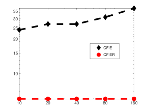
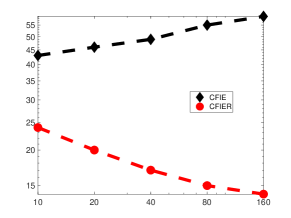
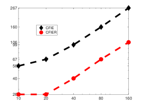
Figure 2: Numbers of GMRES iterations required to reach residuals of $10^{-5}$ for the CFIE and CFIER formulations for the circle (left), kite (middle) and the smooth cavity (right) in the case of Dirichlet boundary conditions and frequencies $\omega=10,20,40,80,160$ with Lamé parameters $\lambda=2$ and $\mu=1$ under plane wave incidence. We used Nyström discretizations corresponding to 8 points per the shorter wavelength. The numbers of iterations are independent of the direction and polarization of the plane wave.

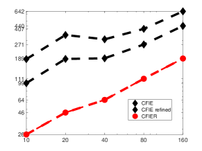
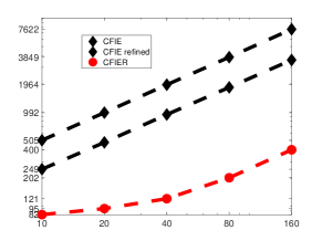
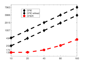
Figure 3: Numbers of GMRES iterations required to reach residuals of $10^{-5}$ for the CFIE and CFIER formulations for the circle (left), kite (middle) and the smooth cavity (right) in the case of Neumann boundary conditions and frequencies $\omega=10,20,40,80,160$ with Lamé parameters $\lambda=2$ and $\mu=1$ under plane wave incidence. We used Nyström discretizations corresponding to 8 points per the shorter wavelength. In order to illustrate the effect of discretization size on the iterative behavior of the CFIE formulations, we report iteration counts ”CFIE refined” corresponding to discretizations refined by a factor of two. The numbers of iterations are independent of the direction and polarization of the plane wave.

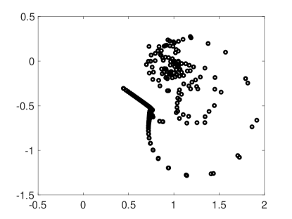
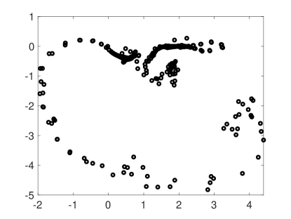
Figure 4: Eigenvalue distribution of the CFIER operators in the case of the kite geometry and $\omega=40$ for the Dirichlet (left) and Neumann (right) cases.

Finally, we illustrate in Figure 5 the iterative behavior of the CFIE and CFIER formulations in the case of Lipschitz scatterers in the high frequency regime. Specifically, we considered a square and an L-shaped scatterer of lengths $2\pi$ with arc length parametrizations, equipped with sigmoidal graded meshes that accumulate points polynomially (e.g. polynomials of degree three were used in our numerical experiments) towards the corner points. We remark that the various well posedness proofs of the formulations considered in this paper relied heavily on the smoothness of the curve $\Gamma$. Indeed, a key ingredient in the analysis was the increased regularity of the double layer operators, that is $\operatorname{K}_{k}^{\top}\in\mathrm{OPS}(-3)$, which in the case of Lipschitz curves is only $\operatorname{K}_{k}^{\top}\in\mathrm{OPS}(0)$. As a consequence, the CFIER formulations are no longer of the second kind. Nevertheless, the CFIER formulations still outperform the CFIE formulations. For instance, we did not observe convergence when GMRES solvers were applied to CFIE formulations in the Neumann case.

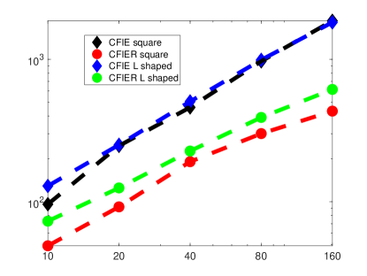
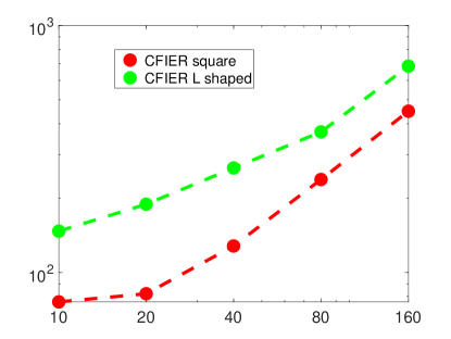
Figure 5: Numbers of GMRES iterations required to reach residuals of $10^{-4}$ for the CFIE and CFIER formulations for the square and the L-shaped scatterers in the high frequency regime for the Dirichlet (left) and Neumann (right) boundary conditions and the same material parameters as in the previous cases, In the case of Neumann boundary conditions, the solvers based on CFIE formulations did not converge.

6 Conclusions

We introduced and analyzed CFIER formulations for the solution of two dimensional elastic scattering problems via Helmholtz decompositions. Despite featuring non standard BIOs, we showed that these CFIER formulations are well posed in the case of smooth scatterers. The CFIER formulations, being of the second kind, possess superior spectral properties to the classical CFIE formulations for both Dirichlet and Neumann boundary conditions. The extension of our approach to the case of homogeneous penetrable scatterers is straightforward and is currently being pursued. The extension of the CFIER methodology to three dimensional elastic scattering problems via Helmholtz decompositions, on the other hand, is more challenging as it requires incorporation of both Helmholtz and Maxwell BIOs.

Appendix A Helmholtz BIOs and pseudodifferential operator calculus

For a given wave-number $k$ and a functional density $\varphi$ on the boundary $\Gamma$ denote in this section the Helmholtz single and double layer potentials in the form

$$\operatorname{SL}_{k,\Gamma}[\varphi]({\bm{x}}):=\int_{\Gamma}H_{0}^{(1)}(k|{\bm{x}}-{\bm{y}}|)\varphi({\bm{y}}){{\rm d}{\bm{y}}},\quad{\operatorname{DL}_{k,\Gamma}}[\varphi]({\bm{x}}):=\int_{\Gamma}\frac{\partial H_{0}^{(1)}(k|{\bm{x}}-{\bm{y}}|)}{\partial\bm{n}({\bm{y}})}\varphi({\bm{y}}){{\rm d}{\bm{y}}},\ {\bm{x}}\in\mathbb{R}^{2}\setminus\Gamma.$$

Any exterior, radiating, solution of the Helmholtz equation can be written

$$u({\bm{x}})=\operatorname{DL}_{k,\Gamma}[\gamma_{\Gamma}^{+}u]({\bm{x}})-\operatorname{SL}_{k,\Gamma}[\partial_{\bm{n}}^{+}u]({\bm{x}}),\quad{\bm{x}}\in\Omega^{+}.$$ (A.1)

The associated layer operators (read by rows in the matrix operator: double layer, single layer, hypersingular and adjoing double layer) are defined as

$$\begin{bmatrix}\gamma^{+}\\ \partial_{\bm{n}}^{+}\end{bmatrix}\begin{bmatrix}\mathrm{DL}_{k,\Gamma}&-\mathrm{SL}_{k,\Gamma}\end{bmatrix}=\begin{bmatrix}\operatorname{K}_{k,\Gamma}&-\operatorname{V}_{k,\Gamma}\\ \operatorname{W}_{k,\Gamma}&-\operatorname{K}^{\top}_{k,\Gamma}\end{bmatrix}=:{\cal C}_{k,\Gamma}:H^{s}(\Gamma)\times H^{s-1}(\Gamma)\to H^{s}(\Gamma)\times H^{s-1}(\Gamma).$$

The matrix operator ${\cal C}_{k,\Gamma}$ is then continuous for any $s$ if $\Gamma$ is smooth. Calderón identities can be derived from the fact that (see for instance [31, Ch.2 ], [22, Ch. 1] or [29, Chapter 6-7]) that

$$\left(\frac{1}{2}\mathcal{I}+{\cal C}_{k,\Gamma}\right)^{2}=\frac{1}{2}\mathcal{I}+{\cal C}_{k,\Gamma},$$

which are equivalent to

$$\operatorname{V}_{k,\Gamma}\operatorname{W}_{k,\Gamma} =-\frac{1}{4}\operatorname{I}+\operatorname{K}_{k,\Gamma}^{2}, \quad\operatorname{W}_{k,\Gamma}\operatorname{V}_{k,\Gamma} =-\frac{1}{4}\operatorname{I}+(\operatorname{K}^{\top}_{k,\Gamma})^{2}$$ (A.2)

$$\operatorname{V}_{k,\Gamma}\operatorname{K}_{k,\Gamma}^{\top} =\operatorname{K}_{k,\Gamma}\operatorname{V}_{k,\Gamma},\quad \operatorname{W}_{k,\Gamma}\operatorname{K}_{k,\Gamma} =\operatorname{K}^{\top}_{k,\Gamma}\operatorname{W}_{k,\Gamma}.$$

It is convenient to present the analysis of robust BIE formulations of Helmholtz decompositions of Navier equations in the framework of periodic pseudodifferential operators. Consider then a regular positive oriented arc-length parameterization of $\Gamma$, ${\bf x}:[0,L]\to\Gamma$ where $L$ is the length of the curve. For any function, or distribution in the general case, $\varphi_{\Gamma}:\Gamma\to\mathbb{C}$ we will denote by

$$\varphi(\tau)=\varphi_{\Gamma}({\bf x}(\tau))$$

its parameterized counterpart. We will extend this convention to the operators. For instance,

$$(\operatorname{V}_{k}\varphi)(\tau)=\frac{i}{4}\int_{0}^{L}H_{0}^{(1)}(k|{\bf x}(t)-{\bf x}(\tau)|)\varphi_{\Gamma}({\bf x}(\tau))\,{\rm d}\tau.$$

is the parameterized version of $\operatorname{V}_{k,\Gamma}$.

The unit tangent and normal parameterized vector to $\Gamma$ (at ${\bf x}(\tau)$) are then given by

$$\bm{t}(\tau)={\bf x}^{\prime}(\tau),\quad\bm{n}(\tau)=\mathrm{Q}{\bf x}^{\prime}(\tau),\quad\mathrm{Q}=\begin{bmatrix}&1\\ -1&\end{bmatrix}$$

so that

$$(\partial_{\bm{t}}\varphi_{\Gamma})\circ{\bf x}=\varphi^{\prime}=:\mathrm{D}\varphi.$$

Besides, the (parameterized) signed quadrature can be then expressed as

$$\kappa=-\bm{t}\cdot\mathrm{D}\bm{n}.$$ (A.3)

It is a well-established result, see for instance [26, Ch. 8], that Sobolev spaces on $\Gamma$ $H^{s}(\Gamma)$ can be then identified with the $L-$periodic Sobolev spaces

$$H^{s}=\Big{\{}\varphi\in{\cal D}^{\prime}(\mathbb{R})\ :\ \varphi(\cdot+L)=\varphi,\quad\|\varphi\|_{s}<\infty\Big{\}}$$

where, with

$$\quad\widehat{\varphi}(n)=\frac{1}{L}\int_{0}^{L}\varphi(\tau)e_{-n}(\tau)\,{\rm d}\tau,\qquad e_{n}(\tau)=\exp\Big{(}\frac{2\pi i}{L}n\tau\Big{)}$$

the Fourier coefficients, the Sobolev norm is given by

$$\|\varphi\|_{s}^{2}=|\widehat{\varphi}(0)|^{2}+\sum_{n\neq 0}|n|^{2s}|\widehat{\varphi}(n)|^{2}.$$

Clearly,

$$\varphi=\widehat{\varphi}(0)+\sum_{n\neq 0}\widehat{\varphi}(n)e_{n}$$

with convergence in $H^{s}$. The set $\{H^{s}\}_{s\in\mathbb{R}}$ is a Hilbert scale, meaning that $H^{s}$ is actually a Hilbert space, that $H^{t}\subset H^{s}$ for any $t>s$ with compact and dense injection and that

$$\bigcap_{s}H^{s}={\cal D}:=\{\varphi\in{\cal C}^{\infty}(\mathbb{R})\ :\ \varphi=\varphi(\cdot+L)\},\quad\bigcup_{s}H^{s}={\cal D}^{\prime}.$$

We will denote by $\mathrm{OPS}(m)$ the class of periodic pseudodifferential operators of order $m\in\mathbb{Z}$ on $\Gamma$. That is, $\mathrm{A}\in\mathrm{OPS}(m)$ if $\mathrm{A}:H^{s}\to H^{s-m}$ is continuous for any $s$. For convenience, we will write that

$$\mathrm{A}=\mathrm{B}+\mathrm{OPS}(m-1),$$

if $\mathrm{A}-\mathrm{B}\in\mathrm{OPS}(m-1)$

Trivially, $\mathrm{A}\in\mathrm{OPS}(m)$ implies that $\mathrm{A}\in\mathrm{OPS}(m+1)$ and as an operator in ${\mathrm{OPS}}(m+1)$ $\mathrm{A}$ is compact. We also set

$${\mathrm{OPS}}(-\infty):=\bigcap_{n\in\mathbb{N}}\mathrm{OPS}(n)$$

the class of smoothing operators which in turn can be identified with integral operators with $L-$periodic smooth kernel.

In connection to periodic pseudodifferential operators, Fourier multipliers will play a central role in what follows:

$$\mathrm{A}\varphi=\sum_{m=-\infty}^{\infty}\mathrm{A}(n)\widehat{\varphi}(n)e_{n}\qquad$$ (A.4)

where $\mathrm{A}(n)\in\mathbb{C}$ are referred to as the symbol of $\mathrm{A}$. Clearly, if $\mathrm{A}$ is a Fourier multiplier defined as in (A.4), if there exists $c>0$ and $r$ such that $|\mathrm{A}(n)|\leq c|n|^{r}$ for all $n\in\mathbb{Z}$ (which for simplicity we shall denote in what follows as $\mathrm{A}(n)=\mathcal{O}(n^{r})$) then $\mathrm{A}\in\mathrm{OPS}(r)$. Equivalently, if

$$\sum_{n\in\mathbb{Z}}|\mathrm{A}(n)|<\infty,$$

then with the function

$$a(t)=\frac{1}{L}\sum_{n\in\mathbb{Z}}\mathrm{A}(n)e_{n}(t)\in L^{\infty}(\mathbb{R}),\quad\text{that is,\quad}\widehat{a}(n)=\frac{1}{L}\mathrm{A}(n),$$

$\mathrm{A}$ is just a convolution operator:

$$\mathrm{A}f=\int_{0}^{L}a(\cdot-\tau)\varphi(\tau)\,{\rm d}\tau.$$

Note that the tangential derivative becomes a Fourier multiplier:

$$\mathrm{D}\varphi=\sum_{n\neq 0}\left(\frac{2\pi im}{L}\right)\widehat{\varphi}(m)e_{m}=\varphi^{\prime}$$

and that for any nonnegative integer $r$,

$$\mathrm{D}^{r}=\mathrm{D}_{r},\quad\mathrm{D}_{r}\varphi:=\sum_{n\neq 0}\left(\frac{2\pi im}{L}\right)^{r}\widehat{\varphi}(m)e_{m}.$$

We will extend this definition to set $\mathrm{D}_{r}$ for negative integer values of $r$ too.

Three additional Fourier multiplier operators we will required in our analysis. First, the Bessel operator

$$\Lambda\varphi = -\frac{1}{2\pi}\int_{0}^{L}\log\left(4e^{-1}\sin^{2}\left(\frac{\pi}{L}(\cdot-\tau)\right)\right)\varphi(\tau)\,{\rm d}\tau=\frac{L}{2\pi}\left[\widehat{\varphi}(0)+\sum_{n\neq 0}\frac{1}{|n|}\widehat{\varphi}(n)e_{n}\right],$$

next, the Hilbert transform, or Hilbert singular operator,

$$\operatorname{H}\varphi:=-\frac{1}{L}\mathrm{p.v.}\int_{0}^{L}\cot\left(\frac{\pi}{L}(\cdot-\tau)\right)\varphi(\tau)\,{\rm d}\tau+i\mathrm{J}\varphi=i\bigg{[}\widehat{\varphi}(0)+\sum_{n\neq 0}\mathop{\rm\rm sign}(n)\widehat{\varphi}(n)e_{n}\bigg{]},$$

with

$$\mathrm{J}\varphi:=\widehat{\varphi}(0)=\frac{1}{L}\int_{\Gamma}\varphi_{\Gamma}.$$

the mean operator. We notice then

$$\mathrm{D}\Lambda =\Lambda\mathrm{D}=i\operatorname{H}+\mathrm{J}, \quad\Lambda =\operatorname{H}\mathrm{D}_{-1}+\frac{L}{2\pi}\mathrm{J},$$

$$\mathrm{D}\mathrm{D}_{-1} =\operatorname{I}-\mathrm{J}=-\operatorname{H}^{2}-\mathrm{J} \quad\Lambda^{-1} =-\mathrm{D}\operatorname{H}+\mathrm{J}=-\mathrm{D}_{2}\Lambda+\frac{2\pi}{L}\mathrm{J}.$$

By a direct analysis of the resulting kernel we can easily check

$$a\operatorname{H}-\operatorname{H}a\in\mathrm{OPS}(-\infty)$$ (A.5)

for any smooth function $a$. Similarly.

$$a\mathrm{D}_{r}-\mathrm{D}_{r}a\in\mathrm{OPS}(r-1)$$ (A.6)

which is trivial to show for positive $r$ and an easy consequence, from negative values of $r$, of the equality

$$\mathrm{D}_{-1}(a\varphi)=a\mathrm{D}_{-1}\varphi-\mathrm{D}_{-1}(a^{\prime}\mathrm{D}_{-1}\varphi)-(\mathrm{D}_{-1}a)\mathrm{J}\varphi.$$

which implies, still for $r<0$

$$\mathrm{D}_{r}(a\varphi)=\sum_{m=-n}^{r}\binom{r}{-m}(\mathrm{D}_{r-m}a)(\mathrm{D}_{m}\varphi)+\mathrm{OPS}(-n-1).$$ (A.7)

We point out that if $\{\operatorname{K}_{0},\operatorname{V}_{0},\operatorname{W}_{0},\operatorname{K}^{\top}_{0}\}$ are the boundary layer operators associated to the Laplace equation ($k=0$),

$$\operatorname{V}_{0} = \frac{1}{2}\Lambda+\mathrm{OPS}(-\infty)=\frac{1}{2}\operatorname{H}\mathrm{D}_{-1}+\mathrm{OPS}(-\infty),$$

$$\operatorname{W}_{0} = -\frac{1}{2}\mathrm{\Lambda}^{-1}_{0}+\mathrm{OPS}(-\infty)=\frac{1}{2}\mathrm{D}\operatorname{H}+\mathrm{OPS}(-\infty)$$

$$\operatorname{K}_{0} = \mathrm{OPS}(-\infty)\ =\operatorname{K}_{0}^{\top}.$$

since the functions

$$\log\left(\frac{\left|\sin\left(\frac{\pi}{L}(t-\tau)\right)\right|}{|{\bf x}(t)-{\bf x}(\tau)|^{2}}\right),\quad\partial_{\tau}\partial_{t}\log\left|\sin\left(\frac{\pi}{L}(t-\tau)\right)\right|-\frac{\bm{n}({\bf x}(t))\cdot\bm{n}({\bf x}(\tau))}{|{\bf x}(t)-{\bf x}(\tau)|^{2}}$$

are smooth.

Our aim is to extend such expansions for the Calderon operators associated to Helmholtz equation. For such purposes, let us define for non-negative integer values of $r$

$$\alpha_{2r}(\tau)=-\frac{1}{2\pi}\left[2\sin^{2}\left(\frac{\pi}{L}\tau\right)\right]^{r}\log\left(4e^{-1}\sin^{2}\left(\frac{\pi}{L}\tau\right)\right)$$

and denote the associated multiplier operator by $\Lambda_{2r}$. Note that $\alpha_{0}(n)=\alpha$, and therefore $\Lambda_{0}=\Lambda$, and that

$$\widehat{\alpha}_{2r}(n)=-\tfrac{1}{2}\widehat{\alpha}_{2r-2}(n-1)+\widehat{\alpha}_{2r-2}(n)-\tfrac{1}{2}\widehat{\alpha}_{2r-2}(n+1)$$

which implies

$$\widehat{\alpha}_{2r}(n)=\frac{(-1)^{r}(2r)!L}{2^{r}(2\pi)}\frac{1}{|n|^{2r+1}}+{\cal O}(n^{-2r-3})=\frac{(-1)^{r}(2r)!2^{r}\pi^{2r}}{L^{2r}}|\widehat{\alpha}_{0}(n)|^{2r+1}+{\cal O}(n^{-2r-3})$$

That is, $\Lambda_{2r}\in\mathrm{OPS}(-2r-1)$ with

$$\Lambda_{2r}=\frac{(2r)!2^{r}\pi^{2r}}{L^{2r}}(-1)^{r}\Lambda^{2r+1}+\mathrm{OPS}(-2r-3).$$

(Actually, $\Lambda_{2r}$ can be expanded in powers of $\Lambda^{2\ell+1}$ with $\ell\geq r$ is needed). In particular,

$$\Lambda_{2}=-\frac{(2\pi)^{2}}{L^{2}}\Lambda^{3}+\mathrm{OPS}(-5).$$

Similarly, we can set

$$\alpha_{2r+1}(\tau)=(e_{1}(\tau)-1)\alpha_{2r}(\tau),$$

show next that

$$\widehat{\alpha}_{2r+1}(n)=\frac{(-1)^{r}(2r+1)!L}{2^{r}(2\pi)}\frac{1}{n^{2r+1}}+{\cal O}(n^{-2r-4}).$$

and conclude that the associated Fourier multiplier operator satisfies

$$\Lambda_{2r+1}=\frac{(2r+1)!2^{r+1}\pi^{2r+1}}{L^{2r+1}}(-1)^{r}\Lambda^{2r+2}+\mathrm{OPS}(-2r-3).$$

Finally, it is a well established result that periodic integral operators

$$\mathrm{L}_{r}\varphi=\int_{0}^{L}D(\cdot,\tau)\alpha_{r}(\cdot-\tau)\varphi(\tau)\,{\rm d}\tau,$$

with $D$ a $L-$periodic smooth function, belongs to $\mathrm{OPS}(-r-1)$ (see [31]).

The well posedness of the various BIE formulations considered in this paper relies heavily on the following result which provides decompositions of the Helmholtz operators $\operatorname{V}_{k}$ and $\operatorname{W}_{k}$ in sums of Fourier multiplier pseudodifferential operators of orders $-1$ and $-3$ for the first operator and $1$ and $-1$ for the second plus remainders that are smoother. Specifically, we establish

Proposition A.1

It holds

$$\operatorname{V}_{k} = \frac{1}{2}\Lambda+\frac{k^{2}}{4}\Lambda^{3}+\mathrm{OPS}(-5),$$ (A.8)

$$\operatorname{W}_{k} = -\frac{1}{2}\Lambda^{-1}+\frac{k^{2}}{4}\Lambda+\mathrm{OPS}(-3),$$ (A.9)

$$\operatorname{K}_{k} = \frac{k^{2}}{2}\kappa\Lambda^{3}+\mathrm{OPS}(-4)=\operatorname{K}_{k}^{\top},$$ (A.10)

Proof. From the decomposition of the Bessel functions (see for instance [26, Ch. 12] or [11, §10]) we get the decomposition:

$$\frac{i}{4}H_{0}^{(i)}(t)=-\frac{1}{4\pi}\log t^{2}+\frac{1}{16\pi}t^{2}\log t^{2}+\underbrace{\frac{1}{4\pi}\frac{1}{t^{4}}(1-\frac{1}{4}t^{2}-J_{0}(t))}_{B_{0}(t)}t^{4}\log t^{2}+C_{0}(t),$$

with $B_{0}$ and $C_{0}$ smooth. Since

$$|{\bf x}(t)-{\bf x}(\tau)|^{2}=\frac{L^{2}}{\pi^{2}}\sin^{2}\left(\frac{\pi}{L}(t-\tau)\right)+D_{1}(t,\tau)\sin^{4}\left(\frac{\pi}{L}(t-\tau)\right),$$

$D_{1}$ being smooth, the following decomposition holds

$$\frac{i}{4}H_{0}^{(i)}(k|{\bf x}(t)-{\bf x}(\tau)|) = -\frac{1}{4\pi}\log\left(4e^{-1}\sin^{2}\left(\frac{\pi}{L}(t-\tau)\right)\right)$$

$$+\frac{(Lk)^{2}}{4}\frac{1}{(2\pi)^{3}}\left(2\sin^{2}\frac{\pi}{L}(t-\tau)\right)\log\left(4e^{-1}\sin^{2}\left(\frac{\pi}{L}(t-\tau)\right)\right)$$

$$+D_{2}(t,\tau)\sin^{4}\left(\frac{\pi}{L}(t-\tau)\right)\log\sin^{2}(4e^{-1}\pi(t-\tau))+D_{3}(t,\tau),$$

where $D_{1},\ D_{2}$ smooth bi-periodic functions. Therefore,

$$\operatorname{V}_{k}\varphi = \frac{1}{2}\Lambda\varphi-\frac{(Lk)^{2}}{4}\frac{1}{(2\pi)^{2}}\int_{0}^{L}\alpha_{2}(\,\cdot\,-\tau)\,\varphi(\tau)\,{\rm d}\tau$$

$$+\int_{0}^{L}D_{2}(t,\tau)\alpha_{4}(\,\cdot\,-\tau)\,\varphi(\tau)\,{\rm d}\tau+\int_{0}^{L}B(\,\cdot\,,\tau)\,\varphi(\tau)\,{\rm d}\tau$$

$$= \frac{1}{2}\Lambda\varphi-\frac{k^{2}}{4}\frac{1}{(2\pi)^{2}}\Lambda_{2}\varphi+\mathrm{OPS}(-5)$$

$$= \frac{1}{2}\Lambda\varphi+\frac{k^{2}}{4}\Lambda^{3}\varphi+\mathrm{OPS}(-5).$$

The analysis of $\mathrm{K}_{k}$ is very similar. Indeed, the kernel is given by

$$\frac{i}{4}H_{1}^{(1)}(k|{\bm{x}}-{\bm{y}}|)k|{\bm{x}}-{\bm{y}}|\frac{({\bm{x}}-{\bm{y}})\cdot\bm{n}({\bm{y}})}{|{\bm{x}}-{\bm{y}}|^{2}},$$

which with the decomposition

$$\frac{i}{4}H_{1}^{(1)}(t)t=-\frac{1}{8\pi}t^{2}\log t^{2}+\underbrace{\frac{1}{4\pi t^{2}}\left(\frac{1}{2}-\frac{1}{t}J_{1}(t)\right)}_{E_{1}(t)}t^{4}\log t^{2}+C_{1}(t).$$

and the fact that

$$\frac{({\bm{x}}-{\bm{y}})\cdot\bm{n}({\bm{y}})}{|{\bm{x}}-{\bm{y}}|^{2}}=-\frac{1}{2}\kappa({\bm{x}})+E_{2}({\bm{x}},{\bm{y}})|{\bm{x}}-{\bm{y}}|$$

($E_{1},\ E_{2}$ are again smooth functions) allow us to write

$$\operatorname{K}_{k}\varphi = -\frac{(Lk)^{2}}{2(2\pi)^{2}}\kappa\Lambda_{2}\varphi+\int_{0}^{L}E_{2}(t,\tau)\alpha_{3}(\,\cdot\,-\tau)\,\varphi(\tau)\,{\rm d}\tau+\int_{0}^{L}E_{3}(\,\cdot\,,\tau)\,\varphi(\tau)\,{\rm d}\tau$$

$$= \frac{k^{2}}{2}\kappa\Lambda^{3}\varphi+\mathrm{OPS}(-4).$$

The case $\operatorname{K}^{\top}$ is consequence of (A.5)-(A.6) since

$$\Lambda(\kappa\cdot)=\kappa\Lambda+\mathrm{OPS}(-2)$$

which with the fact $\Lambda^{\top}=\Lambda$.

Finally, for the hypersingular operator, we note that with the identity $\operatorname{W}_{k}\operatorname{V}_{k}=-\frac{1}{4}\operatorname{I}+(\operatorname{K}_{k}^{\top})^{2}$ cf. (A.2),

$$\operatorname{W}_{k} = \operatorname{W}_{k}\left(\operatorname{I}-\frac{k^{4}}{4}\Lambda^{4}\right)+\mathrm{OPS}(-3)$$

$$= \operatorname{W}_{k}\left(\frac{1}{2}\Lambda+\frac{k^{2}}{4}\Lambda^{3}\right)\left(2\Lambda^{-1}-k^{2}\Lambda\right)+\mathrm{OPS}(-3)$$

$$= \operatorname{W}_{k}\operatorname{V}_{k}\left(2\Lambda^{-1}-k^{2}\Lambda\right)+\underbrace{\operatorname{W}_{k}\left(\frac{1}{2}\Lambda+\frac{k^{2}}{4}\Lambda^{3}-\operatorname{V}_{k}\right)\left(2\Lambda^{-1}-k^{2}\Lambda\right)}_{\in\mathrm{OPS}(-3)}+\mathrm{OPS}(-3)$$

$$= -\frac{1}{4}\left(2\Lambda^{-1}-k^{2}\Lambda\right)+\underbrace{(\operatorname{K}_{k}^{\top})^{2}\left(2\Lambda^{-1}-k^{2}\Lambda\right)}_{\in\mathrm{OPS}(-5)}+\mathrm{OPS}(-3)$$

$$= -\frac{1}{2}\Lambda^{-1}+\frac{k^{2}}{4}\Lambda+\mathrm{OPS}(-3)$$

and the result is proven. $\Box$

Remark A.2

This result appears in a slightly different form [22] (equations (10.4.5)). Indeed, several terms in the asymptotic expansion of the principal symbol of the periodic pseudodifferential operator $\operatorname{V}_{k}$ are provided in equations (10.4.5) in [22], and they coincide with the symbols of the operators in the decomposition we provide in Proposition A.1. Indeed,

It is also evident that the expansions in the four operators for Helmholtz equation can be continued in powers of $\Lambda_{0}$ (or equivalently) $\mathrm{D}\operatorname{H}$), all of them being negative except the first term for $\operatorname{W}_{k}$. Such as expansions have appeared previously in the literature (see for instance [31] and, with applications to the study and design of numerical methods, in [16, 7]).

Theorem A.3

It holds

$$\operatorname{V}_{k} = \operatorname{V}_{0}+2k^{2}\operatorname{V}_{0}^{3}+\mathrm{OPS}(-5)=\frac{1}{2}\operatorname{H}\mathrm{D}_{-1}-\frac{k^{2}}{4}\operatorname{H}\mathrm{D}_{-3}+\mathrm{OPS}(-5),$$ (A.11)

$$\operatorname{W}_{k} = \operatorname{W}_{0}+\frac{k^{2}}{2}\operatorname{V}_{0}+\mathrm{OPS}(-3)=\frac{1}{2}\operatorname{H}\mathrm{D}_{1}+\frac{k^{2}}{4}\operatorname{H}\mathrm{D}_{-1}+\mathrm{OPS}(-3),$$ (A.12)

$$\operatorname{K}_{k} = \operatorname{K}_{k}^{\top}=4k^{2}\kappa\operatorname{V}_{0}^{3}+\mathrm{OPS}(-4)=-\frac{1}{2}\kappa k^{2}\operatorname{H}\mathrm{D}_{-3}+\mathrm{OPS}(-4)$$ (A.13)

Equivalently,

$$\operatorname{V}_{k}\varphi = \frac{L}{4\pi}\sum_{n\neq k}\left(n^{2}-\left(\frac{kL}{2\pi}\right)^{2}\right)^{-1/2}\widehat{\varphi}(n)e_{n}+\mathrm{OPS}(-5),$$ (A.14)

$$\operatorname{W}_{k}\varphi = -\frac{\pi}{L}\sum_{n}\left(n^{2}-\left(\frac{kL}{2\pi}\right)^{2}\right)^{1/2}\widehat{\varphi}(n)e_{n}+\mathrm{OPS}(-3).$$ (A.15)

Finally, the Dirichlet-to-Neumann operator satisfies

$$\mathrm{DtN}_{k}\varphi =\operatorname{H}\mathrm{D}+\frac{k^{2}}{2}\operatorname{H}\mathrm{D}_{-1}-\kappa k^{2}\mathrm{D}_{-2}+\mathrm{OPS}(-4)$$ (A.16)

$$\ =\ \frac{1}{L}\sum_{n}\left(n^{2}-\left(\frac{kL}{2\pi}\right)^{2}\right)^{1/2}\widehat{\varphi}(n)e_{n}+\mathrm{OPS}(-2)=2\operatorname{W}_{k}+\mathrm{OPS}(-2).$$

Proof. Expansions A.11-(A.13) follows from Theorem A.1 whereas Properties (A.14)-(A.15) follows from

$$(n^{2}-k^{2})^{-1/2}=\frac{\operatorname{sign}(n)i}{in}-\frac{\operatorname{sign}(n)i}{(in)^{3}}+{\cal O}(n^{-5}),\quad-(n^{2}-k^{2})^{1/2}=(\operatorname{sign}(n)i)(in)+\frac{\operatorname{sign}(n)i}{in}+{\cal O}(n^{-3}).$$

Finally, if $\operatorname{V}_{k}$ is invertible, using (A.2)

$$\mathrm{DtN}_{k} = \operatorname{V}_{k}^{-1}(-\frac{1}{2}\operatorname{I}+\operatorname{K}_{k})=-4\operatorname{W}_{k}(-\frac{1}{2}\operatorname{I}+\operatorname{K}_{k})+\mathrm{OPS}(-5)$$

$$= 2\operatorname{W}_{k}-4\operatorname{W}_{k}\operatorname{K}_{k}+\mathrm{OPS}(-5).$$

Now (A.16) is straightforward to derive. If $\operatorname{V}_{k}$ fails to be invertible we can use the alternative expression for the Dirichlet-to-Neumann operator

$$\mathrm{DtN}_{k}=\left(\frac{1}{2}\operatorname{I}+\operatorname{K}_{k}^{\top}\right)^{-1}\operatorname{W}_{k}$$

(notice that at least one of $\operatorname{V}_{k}$ or $(\frac{1}{2}\operatorname{I}+\operatorname{K}_{k}^{\top})$ must be invertible) and proceed similarly. $\Box$

Lemma A.4

It holds

$$\bm{n}\cdot\operatorname{W}_{k}(\bm{n}\cdot)=\bm{t}\cdot\operatorname{W}_{k}(\bm{t}\cdot) = -\frac{1}{2}\Lambda^{-1}+\frac{k^{2}}{4}\Lambda+\mathrm{OPS}(-3),$$ (A.17a)

$$\bm{t}\cdot\operatorname{W}_{k}(\bm{n}\cdot)=-\bm{n}\cdot\operatorname{W}_{k}(\bm{t}\cdot) = \frac{1}{2}\kappa\mathrm{D}\Lambda+\frac{k^{2}}{4}\kappa\mathrm{D}\Lambda^{3}+\mathrm{OPS}(-3),$$ (A.17b)

$$\bm{n}\cdot\operatorname{V}_{k}(\bm{n}\cdot)=\bm{t}\cdot\operatorname{V}_{k}(\bm{t}\cdot) = \frac{1}{2}\Lambda+\frac{1}{4}(2\kappa+k^{2})\Lambda^{3}+\mathrm{OPS}(-4),\$$ (A.17c)

$$\bm{t}\cdot\operatorname{V}_{k}(\bm{n}\cdot)=\bm{n}\cdot\operatorname{V}_{k}(\bm{t}\cdot) = -\frac{1}{2}\kappa\mathrm{D}\Lambda^{3}+\mathrm{OPS}(-4),\$$ (A.17d)

$$\bm{n}\cdot\mathrm{D}\operatorname{V}_{k}(\bm{n}\cdot)=\bm{t}\cdot\mathrm{D}\operatorname{V}_{k}(\bm{t}\cdot) = \frac{1}{2}\mathrm{D}\Lambda+\frac{k^{2}}{4}\mathrm{D}\Lambda^{3}+\mathrm{OPS}(-4),\$$ (A.17e)

$$\bm{t}\cdot\mathrm{D}\operatorname{V}_{k}(\bm{n}\cdot)=-\bm{n}\cdot\mathrm{D}\operatorname{V}_{k}(\bm{t}\cdot) = -\frac{k^{2}}{2}\kappa\Lambda^{3}+\mathrm{OPS}(-4).$$ (A.17f)

Proof. We start from the identities

$${\bm{n}}\cdot\mathrm{D}_{2}\bm{n}={\bm{t}}\cdot\mathrm{D}_{2}{\bm{t}} =\ \mathrm{D}_{2}-\kappa^{2}\operatorname{I},$$ (A.18)

$${\bm{n}}\cdot\mathrm{D}_{2}{\bm{t}}=-{\bm{t}}\cdot\mathrm{D}_{2}\bm{n} =\ -2\kappa\mathrm{D}+\kappa^{\prime}\,\operatorname{I},\$$

$${\bm{n}}\cdot\mathrm{D}\bm{n}=-{\bm{t}}\cdot\mathrm{D}{\bm{t}} =\ \mathrm{D},\$$

$${\bm{t}}\cdot\mathrm{D}\bm{n}=-{\bm{n}}\cdot\mathrm{D}{\bm{t}} =\ \kappa\operatorname{I},\$$

$${\bm{n}}\cdot\mathrm{D}_{-1}\bm{n}={\bm{t}}\cdot\mathrm{D}_{-1}{\bm{t}} =\ \mathrm{D}_{-1}-\kappa\mathrm{D}_{-3}+(1+\kappa)(\mathrm{D}\kappa)\mathrm{D}_{-4}+\mathrm{OPS}(-5),\$$

$${\bm{t}}\cdot\mathrm{D}_{-1}\bm{n}=-{\bm{n}}\cdot\mathrm{D}_{-1}{\bm{t}} =\ -\kappa\mathrm{D}_{-2}+\kappa^{\prime}\,\mathrm{D}_{-3}+(\mathrm{D}^{2}\kappa-\kappa^{2})\mathrm{D}_{-4}+\mathrm{OPS}(-5),\$$

$${\bm{n}}\cdot\mathrm{D}_{-2}\bm{n}={\bm{t}}\cdot\mathrm{D}_{-2}{\bm{t}} =\ \mathrm{D}_{-2}+3\kappa^{2}\mathrm{D}_{-4}+\mathrm{OPS}(-5),\$$

$${\bm{t}}\cdot\mathrm{D}_{-2}\bm{n}=-{\bm{n}}\cdot\mathrm{D}_{-2}{\bm{t}} =\ -2\kappa\mathrm{D}_{-3}-3\kappa^{\prime}\,\mathrm{D}_{-4}+\mathrm{OPS}(-4)$$

which can be easily proven from (A.3). Hence the result follows from Proposition A.1 and the commutation properties for $\operatorname{H}$ cf. (A.5), the Leibnitz rule for the derivatives and its extension cf. (A.7) for the negative order derivatives $\mathrm{D}_{-r}$. $\Box$

Theorem A.5

It holds

$$\bm{n}\cdot\operatorname{W}_{k}(\bm{n}\cdot)=\bm{t}\cdot\operatorname{W}_{k}(\bm{t}\cdot) = \operatorname{W}_{k}+\mathrm{OPS}(-3)$$ (A.19a)

$$= \frac{1}{2}\mathrm{D}\operatorname{H}+\frac{k^{2}}{4}\operatorname{H}\mathrm{D}_{-1}+\mathrm{OPS}(-3)$$

$$\bm{t}\cdot\operatorname{W}_{k}(\bm{n}\cdot)=-\bm{n}\cdot\operatorname{W}_{k}(\bm{t}\cdot) = \kappa\mathrm{D}\operatorname{V}_{k}+\mathrm{OPS}(-3)$$ (A.19b)

$$= \frac{1}{2}\kappa\operatorname{H}-\frac{k^{2}}{4}\kappa\mathrm{D}_{-2}\operatorname{H}+\mathrm{OPS}(-4)$$

$$\bm{n}\cdot\operatorname{V}_{k}(\bm{n}\cdot)=\bm{t}\cdot\operatorname{V}_{k}(\bm{t}\cdot) = \operatorname{V}_{k}+4\kappa\operatorname{V}_{k}^{3}+\mathrm{OPS}(-4)$$ (A.19c)

$$= \frac{1}{2}\operatorname{H}\mathrm{D}_{-1}-\frac{1}{4}(k^{2}+2\kappa)\mathrm{D}_{-3}\operatorname{H}+\mathrm{OPS}(-3)$$

$$\bm{t}\cdot\operatorname{V}_{k}(\bm{n}\cdot)=-\bm{n}\cdot\operatorname{V}_{k}(\bm{t}\cdot) = -4\kappa\operatorname{V}_{k}^{3}+\mathrm{OPS}(-4)$$ (A.19d)

$$= \frac{1}{2}\kappa\mathrm{D}_{-3}\operatorname{H}+\mathrm{OPS}(-4)\$$

$$\bm{n}\cdot\mathrm{D}\operatorname{V}_{k}(\bm{n}\cdot)=\bm{t}\cdot\mathrm{D}\operatorname{V}_{k}(\bm{t}\cdot) = \mathrm{D}\operatorname{V}_{k}+\mathrm{OPS}(-4)$$ (A.19e)

$$= \frac{1}{2}\operatorname{H}-\frac{k^{2}}{4}\mathrm{D}_{-2}\operatorname{H}+\mathrm{OPS}(-4)\$$

$$\bm{t}\cdot\mathrm{D}\operatorname{V}_{k}(\bm{n}\cdot)=-\bm{n}\cdot\mathrm{D}\operatorname{V}_{k}(\bm{t}\cdot) = -4k^{2}\kappa\mathrm{D}\operatorname{V}_{k}^{3}+\mathrm{OPS}(-4)$$ (A.19f)

$$= \frac{1}{2}k^{2}\kappa\operatorname{H}\mathrm{D}_{-2}+\mathrm{OPS}(-4)$$

$$\bm{n}\cdot\operatorname{K}_{k}(\bm{n}\cdot)=\bm{t}\cdot\operatorname{K}_{k}(\bm{t}\cdot) = 4k^{2}\kappa\operatorname{V}_{k}^{3}+\mathrm{OPS}(-4)$$ (A.19g)

$$= -\frac{1}{2}k^{2}\kappa\operatorname{H}\mathrm{D}_{-3}+\mathrm{OPS}(-4)\$$

$$\bm{t}\cdot\operatorname{K}_{k}(\bm{n}\cdot)=-\bm{n}\cdot\operatorname{K}_{k}(\bm{t}\cdot) = \mathrm{OPS}(-4).$$ (A.19h)

Proof. It is consequence of Lemma A.4 and Proposition A.1. $\Box$

References

[1]
H. Ammari, H. Kang, and H. Lee.
Layer potential techniques in spectral analysis, volume 153 of
Mathematical Surveys and Monographs.
American Mathematical Society, Providence, RI, 2009.
[2]
Y. Boubendir, O. Bruno, C. Levadoux, and C. Turc.
Integral equations requiring small numbers of Krylov-subspace
iterations for two-dimensional smooth penetrable scattering problems.
Appl. Numer. Math., 95:82–98, 2015.
[3]
Y. Boubendir, V. Domínguez, D. Levadoux, and C. Turc.
Regularized combined field integral equations for acoustic
transmission problems.
SIAM Journal on Applied Mathematics, 75(3):929–952, 2015.
[4]
H. Brakhage and P. Werner.
Über das Dirichletsche Aussenraumproblem für die
Helmholtzsche Schwingungsgleichung.
Arch. Math., 16:325–329, 1965.
[5]
O. P. Bruno and T. Yin.
Regularized integral equation methods for elastic scattering problems
in three dimensions.
Journal of Computational Physics, 410:109350, 2020.
[6]
A.J. Burton and G.F. Miller.
The application of integral equation methods to the numerical
solution of some exterior boundary-value problems.
Proc. Roy. Soc. London. Ser. A, 323:201–210, 1971.
A discussion on numerical analysis of partial differential equations
(1970).
[7]
R. Celorrio, V. Domínguez, and F.J. Sayas.
Periodic Dirac delta distributions in the boundary element method.
Adv. Comput. Math., 17(3):211–236, 2002.
[8]
S. Chaillat, M. Darbas, and F. Le Louër.
Approximate local Dirichlet-to-Neumann map for three-dimensional
time-harmonic elastic waves.
Computer Methods in Applied Mechanics and Engineering,
297:62–83, 2015.
[9]
S. Chaillat, M. Darbas, and F. Le Louër.
Analytical preconditioners for Neumann elastodynamic boundary
element methods.
Partial Differ. Equ. Appl., 2(2):Paper No. 22, 26, 2021.
[10]
R. Chapko, R. Kress, and L. Monch.
On the numerical solution of a hypersingular integral equation for
elastic scattering from a planar crack.
IMA journal of numerical analysis, 20(4):601–619, 2000.
[11]NIST Digital Library of Mathematical Functions.
http://dlmf.nist.gov/, Release 1.1.2 of 2021-06-15.
F. W. J. Olver, A. B. Olde Daalhuis, D. W. Lozier, B. I. Schneider,
R. F. Boisvert, C. W. Clark, B. R. Miller, B. V. Saunders, H. S. Cohl, and
M. A. McClain, eds.
[12]
V. Domínguez, S.L. Lu, and F.J. Sayas.
A fully discrete Calderón calculus for two dimensional time
harmonic waves.
Int. J. Numer. Anal. Model., 11(2):332–345, 2014.
[13]
V. Domínguez, S.L. Lu, and F.J. Sayas.
A Nyström flavored Calderón calculus of order three for
two dimensional waves, time-harmonic and transient.
Computers & Mathematics with Applications, 67(1):217–236,
2014.
[14]
V. Domínguez, M.L. Rapún, and F.J. Sayas.
Dirac delta methods for Helmholtz transmission problems.
Advances in Computational Mathematics, 28(2):119–139, 2008.
[15]
V. Domínguez, T. Sánchez-Vizuet, and F.J. Sayas.
A fully discrete Calderón calculus for the two-dimensional
elastic wave equation.
Comput. Math. Appl., 69(7):620–635, 2015.
[16]
V. Domínguez and F.J. Sayas.
An asymptotic series approach to Qualocation methods.
J. Integral Equations Appl., 15(2):113–151, 2003.
[17]
V. Domínguez and C. Turc.
Boundary integral equation methods for the solution of scattering and
transmission 2D elastodynamic problems.
IMA J. Appl. Math., 87(4):647–706, 2022.
[18]
V. Domínguez and C. Turc.
Nystrom discretizations of boundary integral equations for the
solution of 2D elastic scattering problems.
arXiv preprint arXiv:2206.11965, 2022.
[19]
H. Dong, J. Lai, and P. Li.
A highly accurate boundary integral method for the elastic obstacle
scattering problem.
Mathematics of Computation, (90):2785–2814, 2021.
[20]
H Dong, J. Lai, and P. Li.
A spectral boundary integral method for the elastic obstacle
scattering problem in three dimensions.
Journal of Computational Physics, 469:111546, 2022.
[21]
L. M. Faria, C. Pérez-Arancibia, and M. Bonnet.
General-purpose kernel regularization of boundary integral equations
via density interpolation.
Computer Methods in Applied Mechanics and Engineering,
378:113703, 2021.
[22]
G.C. Hsiao and W.L. Wendland.
Boundary integral equations.
Springer, 2008.
[23]
A. Klöckner, A. Barnett, L. Greengard, and M. Neil.
Quadrature by expansion: A new method for the evaluation of layer
potentials.
Journal of Computational Physics, 252:332–349, 2013.
[24]
P. Kolm, S. Jiang, and V. Rokhlin.
Quadruple and octuple layer potentials in two dimensions i:
Analytical apparatus.
Applied and Computational Harmonic Analysis, 14(1):47–74,
2003.
[25]
R. Kress.
On the numerical solution of a hypersingular integral equation in
scattering theory.
J. Comput. Appl. Math., 61(3):345–360, 1995.
[26]
R. Kress.
Linear integral equations, volume 82 of Applied
Mathematical Sciences.
Springer-Verlag, New York, second edition, 1999.
[27]
V.D. Kupradze.
Three-dimensional problems of elasticity and thermoelasticity.
Elsevier, 2012.
[28]
J. Lai and P. Li.
A framework for simulation of multiple elastic scattering in two
dimensions.
SIAM Journal on Scientific Computing, 41(5):A3276–A3299, 2019.
[29]
W. McLean.
Strongly elliptic systems and boundary integral equations.
Cambridge University Press, Cambridge, 2000.
[30]
Y. Saad and M.H. Schultz.
GMRES: a generalized minimal residual algorithm for solving
nonsymmetric linear systems.
SIAM J. Sci. Statist. Comput., 7(3):856–869, 1986.
[31]
J. Saranen and G. Vainikko.
Periodic integral and pseudodifferential equations with
numerical approximation.
Springer Monographs in Mathematics. Springer-Verlag, Berlin, 2002.