Estimation of Systemic Shortfall Risk Measure using Stochastic Algorithms

Abstract

Systemic risk measures were introduced to capture the global risk and the corresponding contagion effects that is generated by an interconnected system of financial institutions. To this purpose, two approaches were suggested. In the first one, systemic risk measures can be interpreted as the minimal amount of cash needed to secure a system after aggregating individual risks. In the second approach, systemic risk measures can be interpreted as the minimal amount of cash that secures a system by allocating capital to each single institution before aggregating individual risks. Although the theory behind these risk measures has been well investigated by several authors, the numerical part has been neglected so far. In this paper, we use stochastic algorithms schemes in estimating MSRM and prove that the resulting estimators are consistent and asymptotically normal. We also test numerically the performance of these algorithms on several examples.

Keywords: Multivariate risk measures, shortfall risk, stochastic algorithms, stochastic root finding, risk allocations.

Introduction

The axiomatic theory of risk measures, first initiated by the seminal paper of Artzner et al. (1999), has been widely studied during the last years. Value-at-Risk(VaR) is one of the most known and common risk measures used by practitioners and regulation authorities. However, VaR lacks one important property: it does not take into account the diversification effect. To circumvent this problem, the VaR was replaced by the Conditional Value-at-Risk (CVaR) and a more general framework of improved risk measures has been introduced: Utility-based Shortfall Risk (SR). Nevertheless, when it comes to a system of financial institutions or portfolios, the question about how to assess the global risk as well as individual risks arise. Following the 2008 crisis, the traditional approach of measuring systemic risk that consists in considering each institution as a single entity isolated from other institutions, has shown its own limits. Indeed, with this approach, the risk associated to a vector of positions $X=(X_{1},...,X_{d})$ can be written as:

$$R(X)\vcentcolon=\sum_{i=1}^{d}\eta_{i}(X_{i}),$$

where each $\eta_{i}$ is a univariate risk measure. Then, Chen et al. (2013) proposed an approach that is very close in spirit to the axiomatic framework initiated by Artzner et al. (1999). They showed that any systemic risk measure verifying certain axioms is the composition of a univariate risk measure $\eta$ and an aggregation $\Lambda$, i.e.,

$$R(X)=\eta(\Lambda(X)).$$

The previous representation is known as the “Aggregate then Add Cash” approach as it consists first in aggregating the positions $X_{1},...,X_{d}$ through the aggregation function $\Lambda$ and then to apply a univariate risk measure. One of the most common ways to aggregate the outcomes $X_{i}$ is to simply take the sum, that is to consider, $\Lambda(x)=\sum_{i=1}^{d}x_{i}$. It is worth noticing that, while summing up profit and losses might seem reasonable from the point of view of a portfolio manager because portfolios profits and losses compensate each other, this aggregation rule seems inadequate from the point of view of a regulator where cross-subsidization between institutions is not realistic since no institution will be willing to pay for the losses of another one.
Motivated by these considerations, Biagini et al. (2019) proposed another approach to measure the systemic risk. They first considered the systemic risk as the minimal capital that secures the system by injecting capital into the single institutions, before aggregating the individual risks:

$$R(X)\vcentcolon=\inf\{\sum_{i=1}^{d}m_{i},\leavevmode\nobreak\ \Lambda(X+m)\in\mathbb{A}\},$$ (0.1)

where $\mathbb{A}$ is an acceptance set. This approach, known as “Add Cash then Aggregate” consists in adding the amount $m_{i}$ to the financial position $X_{i}$ before the corresponding total loss $\Lambda(X+m)$ is computed. The systemic risk is then measured as the minimal total amount $\sum_{i=1}^{d}m_{i}$ injected into the institutions to make it acceptable. With this approach, a joint measure of total risk as well as individuals risk contributions to systemic risk is obtained. If $m^{*}=(m_{1}^{*},...,m_{d}^{*})$ is an optimum, that is $R(X)=\sum_{i=1}^{d}m_{i}^{*}$ and $\Lambda(X+m^{*})\in\mathbb{A}$, one could order the $m_{i}^{*}$’s and hence be able to say that institution $i$ requires more cash allocation or is riskier that institution $j$ if $m_{i}^{*}\geq m_{j}^{*}$.
In this article, we are interested in the numerical approximation of the multivariate shortfall risk measure (MSRM) that was introduced in Armenti et al. (2018). They are an extension of univariate SR and can be obtained by taking the aggregation function $\Lambda(x)=l_{S}(-x)$ where $l_{S}$ is a multivariate loss function (see Section 1) and the acceptance set $\mathbb{A}=\{X\in L^{0}(\mathbb{R}),E[X]\leq 0\}$.
To meet the regulatory requirements, financial institutions need to develop a reliable risk management framework to face all kind of financial risks associated to their portfolios. Most of the time, financial institutions use the standard VaR and CVaR although it suffers from some deficiencies. The most common method used to compute VaR is the inversion of the simulated empirical P&L distribution function using Monte Carlo or historical simulation tools (see Glasserman (2004) and Glasserman et al. (2008)). Another idea to compute VaR and CVaR comes from the fact that they are solutions and the value of the same convex optimization problem as pointed out in Rockafellar and Uryasev (2000). Moreover, as they can be expressed as an expectation, this led Bardou et al. (2009) to define consistent and asymptotically normal estimators of both quantities using a classical Robbins-Monro (RM) procedure. Since VaR and CVaR are both related to the simulation of rare events, they also introduced a recursive and adaptive variance method based on importance sampling paradigm.
RM algorithms have been the subject of an enormous literature, both theoretical and applied. The basic paradigm in its simplest form is the following stochastic difference equation: $Z_{n+1}=Z_{n}+\gamma_{n}Y_{n}$, where $Z_{n}$ takes its values in some Euclidean space, $Y_{n}$ is a noisy observable variable, and $\gamma_{n}>0$ is the step size that goes to zero as $n\rightarrow\infty$. The original work was motivated by the classic problem of finding a root of a continuous function $z\to g(z)$, which is unknown but such that, we are able to take only “noisy” measurements at any desired value $z$. This is the case when the function $g$ can be expressed as an expectation, that is $g(z)=E[G(X,z)]$, where $X$ is some random variable. In such situation, the noisy observation variable is simply $Y_{n}=G(X_{n+1},Z_{n})$, where $(X_{n})$ is a sequence of i.i.d random variables with the same law as $X$. If moreover, the random variable $X$ is not directly simulatable, but can only be approximated by another easily simulatable random variable, Frikha (2016) recently extended the scope of multi-level Monte Carlo to the framework of stochastic algorithms and proved central limit theorems.
In many cases, the analysis of these algorithms uses the so-called ODE (Ordinary Differential Equation) method introduced by Ljung (1977). The main idea is to show that, in the long run, the noise is eliminated so that, asymptotically, the behaviour of the algorithm is determined by that of the “mean” ODE: $\dot{z}=g(z)$. An introductory approach to RM algorithms and their convergence rate can be found in Duflo (1996) and Benveniste et al. (1990). To ensure the convergence of RM algorithms to the root of the function $g$, it does not require too restrictive assumptions except for one: the sub-linear growth of the function $g$. One way to deal with this restrictive assumption is to use projection techniques. This consists in using the projection into a compact $K$ each time the sequence $Z_{n}$ goes out of $K$. This procedure was first introduced by Kushner and Sanvicente (1975) in order to deal with problems of convex optimization with constraints. Another way to deal with this constraint in the framework of variance reduction using importance sampling method was proposed in Lemaire and Pagès (2010). They have showed that under some regularity assumption on the density of the law of $X$, we can obtain almost-surely convergence result and central limit theorems. In this paper, for the sake of simplicity, we will rather use projection techniques. An excellent survey on projection techniques, their links with ordinary differential equation (ODE) and stochastic algorithms can be found in Kushner and Yin (2003).
SR can be characterized as the unique root of a function $g:\mathbb{R}\mapsto\mathbb{R}$ that is expressed as an expectation. Therefore, a straightforward approach for estimating SR consists in, first, using a deterministic root finding algorithm that would converge to the root, and second, designing an efficient Monte Carlo procedure that estimates $g(s)$ at each given argument $s\in\mathbb{R}$. One could also use variance reduction techniques in order to accelerate the estimation of the function $g$ at each argument $s\in\mathbb{R}$. This idea is very close to sample average methods in stochastic programming. For more details, see, for example, Kleywegt et al. (2001), Linderoth et al. (2006), Mak et al. (1999), Shapiro and Nemirovski (2005), Verweij et al. (2003a) and Verweij et al. (2003b). An alternative to this combination of Monte Carlo method and deterministic root finding schemes is to use stochastic algorithm as presented in Dunkel and Weber (2010). In their work, they did not assume the sub-linear growth of the function $g$, and therefore used projection techniques to prevent the algorithm from explosion.
In this paper, we will see that the optimal allocations of multivariate shortfall risk measures can also be characterized as the root of a function that is expressed as an expectation. More precisely, the optimal allocations are characterized as the solution of the first order condition of the Lagrangian associated to the multivariate risk measure. Again, because we do not want to reduce drastically the scope of application, we will use stochastic algorithms with projection to approximate the optimal allocations.
The paper is organized as follows. The next section, is dedicated to MSRM and the definitions related to them. The main theorem that characterizes the optimal allocations for MSRM is presented. In Section 2, we explain the ODE method and recall some stability results that we will use later to establish convergence results. Finally, section 3 is devoted to some numerical experiments of our procedures. We present a first testing example with an exponential loss function, where we have a closed formula for optimal allocations. We also give a second example using a loss function with a mixture of positive part and quadratic functions.

1 About Multivariate Risk Measures

Let $(\Omega,\mathcal{F},P)$ be a probability space, and denote by $L^{0}(\mathbb{R}^{d})$ the space of $\mathcal{F}$-measurable $d$-variate random variables on this space with $d\geq 2$. For $x,y\in\mathbb{R}^{d}$, we say that that $x\geq y$ ( $x>y$ resp.) if $x_{k}\geq y_{k}$ ($x_{k}>y_{k}$ resp.) for every $1\leq k\leq d$. We denote by $||\cdot||$ the Euclidean norm, and $x\cdot y=\sum x_{k}y_{k}$. For a function $f:\mathbb{R}^{d}\mapsto[-\infty,\infty]$, we denote by $f^{*}(y)=\sup_{x}\{x\cdot y-f(x)\}$ the convex conjugate of $f$. The space $L^{0}(\mathbb{R}^{d})$ inherits the lattice structure of $\mathbb{R}^{d}$ and therefore, we can use the classical notations in $\mathbb{R}^{d}$ in a $P$-almost-sure sens. We say, for example, for $X,Y\in L^{0}(\mathbb{R}^{d})$, that $X\geq Y$ (or $X>Y$ resp.) if $P(X\geq Y)=1$ (or $P(X>Y)=1$ resp.). To simplify the notation, we will simply write $L^{0}$ instead of $L^{0}(\mathbb{R}^{d})$. Now, let $X=(X_{1},...,X_{d})\in L^{0}$ be a random vector of financial losses, i.e., negative values of $X_{k}$ represents actually profits. We want to assess the systemic risk of the whole system and to determine a monetary risk measure, which will be denoted $R(X)$, as well as a risk allocation $RA_{k}(X),k=1,...,d$ among the $d$ risk components. Inspired by the univariate case introduced in Föllmer and Schied (2002), Armenti et al. (2018) introduced a multivariate extension of shortfall risk measures by the means of loss functions and sets of acceptable monetary risk allocations.

Definition 1.1.

A function $l:\mathbb{R}^{d}\mapsto(-\infty,\infty]$ is called a loss function if:

1. $l$ is increasing, that is $l(x)\geq l(y)$ if $x\geq y$;

2. $l$ is convex and lower-semicontinuous with $\inf l<0$;

3. $l(x)\geq\sum x_{k}-c$ for some constant $c$.

Furthermore, a loss function $l$ is said to be permutation invariant if $l(x)=l(\pi(x))$ for every permutation $\pi$ of its components.

Comment: The property (A1) expresses the normative fact about the risk, that is, the more losses we have, the riskier is our system. As for (A2), it expresses the desired property of diversification. Finally, (A3) says that the loss function put more weight on high losses than a risk neutral evaluation.

Example 1.

Let $h:\mathbb{R}\mapsto\mathbb{R}$ be one dimensional loss function satisfying condition (A1), (A2) and (A3). We could build a multivariate loss function using this one dimensional loss function in the following way:

1. $l(x)=h(\sum x_{k})$;

2. $l(x)=\sum h(x_{k})$;

3. $l(x)=\alpha h(\sum x_{k})+(1-\alpha)\sum h(x_{k})$ for $0\leq\alpha\leq 1$.

More specifically, in (C1), we are aggregating losses before evaluating the risk, whereas in (C2), we evaluate individual risks before aggregating. The loss function in (C3) is a convex combination of those in (C1) and (C2).
One of the main examples we will be studying in this paper are the two following ones:

$$h(x)=\frac{1}{\alpha+1}(\sum_{i}e^{\beta x_{i}}+\alpha e^{\beta\sum x_{i}})-\frac{\alpha+d}{\alpha+1},\leavevmode\nobreak\ \leavevmode\nobreak\ h(x)=\sum_{i}x_{i}+\frac{1}{2}\sum_{i}(x_{i}^{+})^{2}+\alpha\sum_{i<j}x_{i}^{+}x_{j}^{+},$$

where the coefficient $\alpha>0$ is called the systemic weight and $\beta>0$ is a risk aversion coefficient.
In the following, we will consider multivariate risk measures defined on Orlicz spaces (see Rao and Ren (1991) for further details on the theory of Orlicz spaces). This has several advantages. From a mathematical point of view, it is a more general setting than $L^{\infty}$, and in the same time, it simplifies the analysis especially for utility maximization problems. Therefore, we will consider loss vectors in the following multivariate Orlicz heart:

$$M^{\theta}=\{X\in L^{0}:\leavevmode\nobreak\ E[\theta(\lambda X)]<\infty,\leavevmode\nobreak\ \forall\lambda>0\},$$

where $\theta(x)=l(|x|),x\in\mathbb{R}^{d}$. See Appendix in Armenti et al. (2018) for more details about Orlicz spaces.
Next, we give the definition of multivariate shortfall risk measures as it was introduced in Armenti et al. (2018).

Definition 1.2.

Let $l$ be a multivariate loss function and $X\in M^{\theta}$, we define the acceptance set $\mathcal{A}(X)$ by:

$$\mathcal{A}(X)\vcentcolon=\{m\in\mathbb{R}^{d}:\leavevmode\nobreak\ E[l(X-m)]\leq 0\}.$$

The multivariate shortfall risk of $X\in M^{\theta}$ is defined as:

$$R(X)\vcentcolon=\inf\left\{\sum m_{k}:\leavevmode\nobreak\ m\in\mathcal{A}(X)\right\}=\inf\left\{\sum m_{k}:\leavevmode\nobreak\ E[l(X-m)]\leq 0\right\}.$$ (1.1)

Remark 1.3.

When $d=1$, the above definition corresponds exactly to the univariate shortfall risk measure in Föllmer and Schied (2002).

The following theorem from Armenti et al. (2018) shows that the multivariate shortfall risk measure has the desired properties and admits a dual representation as in the case of univariate shortfall risk measure. We introduce $Q^{\theta^{*}}$ the set of measure densities in $L^{\theta^{*}}$, the dual space of $M^{\theta}$:

$$Q^{\theta^{*}}\vcentcolon=\left\{\frac{dQ}{dP}\vcentcolon=(Z_{1},...,Z_{d}),\leavevmode\nobreak\ Z\in L^{\theta^{*}},\leavevmode\nobreak\ Z_{k}\geq 0\leavevmode\nobreak\ \text{and}\leavevmode\nobreak\ E[Z_{k}]=1\leavevmode\nobreak\ \text{for every k}\right\}.$$

Theorem 1.4.

[Theorem 2.10 in Armenti et al. (2018)] The function

$$R(X)\vcentcolon=\inf\left\{\sum m_{k}:\leavevmode\nobreak\ m\in\mathcal{A}(X)\right\},$$

is real-valued, convex, monotone and translation invariant. Moreover, it admits the dual representation:

$$R(X)=\underset{Q\in Q^{\theta^{*}}}{\max}\{E_{Q}[X]-\alpha(Q)\},\leavevmode\nobreak\ \leavevmode\nobreak\ X\in M^{\theta},$$

where the penalty function is given by

$$\alpha(Q)=\underset{\lambda>0}{\inf}\leavevmode\nobreak\ E\left[\lambda l^{*}\left(\frac{dQ}{\lambda dP}\right)\right],\leavevmode\nobreak\ \leavevmode\nobreak\ Q\in Q^{\theta^{*}}.$$

Now, we address the question of existence and uniqueness of a risk allocation which are not straightforward in the multivariate case. Armenti et al. (2018) showed that if the loss function is permutation invariant, then risk allocations exist and they are characterized by Kuhn-Tucker conditions. We denote by $Z=\{m\in\mathbb{R}^{d},\sum m_{i}=0\}$ the zero-sum allocations set.

Definition 1.5.

A risk allocation is an acceptable monetary risk allocation $m\in\mathcal{A}(X)$ such that $R(X)=\sum m_{k}$. When a risk allocation is uniquely determined, we denote it by $RA(X)$.

We make the following assumption on the loss function $l$ and the vector of losses $X\in M^{\theta}$:

1. 1. For every $m_{0}$, $m\mapsto l(X-m)$ is differentiable at $m_{0}$ a.s.;

   2. $l$ is permutation invariant.

Theorem 1.6.

[Theorem 3.4 in Armenti et al. (2018)] Let $l$ be a loss function and $X\in M^{\theta}$ such that assumption ($\mathcal{A}$_l) holds. Then, risk allocations $m^{*}\in\mathbb{R}^{d}$ exists and they are characterized by the first order conditions:

$$1=\lambda^{*}\mathbb{E}[\nabla l(X-m^{*})],\leavevmode\nobreak\ \leavevmode\nobreak\ \leavevmode\nobreak\ \mathbb{E}[l(X-m^{*})]=0,$$

where $\lambda^{*}\geq 0$ is a Lagrange multiplier. If moreover $l(x+\cdot)$ is strictly convex along zero sum allocations for every $x$ such that $l(x)\geq 0$, the risk allocation is unique.

Comment: Let $f_{0}(m)=\sum_{i=1}^{d}m_{i}$ and $f_{1}(m)\vcentcolon=E[l(X-m)]$, for $m\in\mathbb{R}^{d}$ and $X\in M^{\theta}$. The assumption ($\mathcal{A}$_l)-($\mathcal{A}$_l)i. together with the convexity of the function $m\mapsto l(X-m)$, we have that, by Theorem 7.46 in Shapiro et al. (2009), $f_{1}$ is differentiable at every $m\in\mathbb{R}^{d}$ and that,

$$\nabla f_{1}(m)=-E[\nabla l(X-m)],\leavevmode\nobreak\ m\in\mathbb{R}^{d}.$$

Therefore, the first order conditions given in the above theorem are equivalent to :

$$\left\{\begin{aligned} &\nabla f_{0}(m^{*})+\lambda^{*}\nabla f_{1}(m^{*})=0,\\ &\lambda^{*}f_{1}(m^{*})=0.\end{aligned}\right.$$

Furthermore, we also know, thanks to Theorem 28.3 in Rockafellar (1970), that the above conditions are equivalent to saying that $(m^{*},\lambda^{*})$ is a saddle point of the Lagrangian associated to the problem in (1.1), i.e.,

$$L(m,\lambda)\vcentcolon=f_{0}(m)+\lambda f_{1}(m)=\sum_{i=1}^{d}m_{i}+\lambda E[l(X-m)].$$ (1.2)

Under the assumptions of the above theorem $z^{*}\vcentcolon=(m^{*},\lambda^{*})$ is the unique solution of $h(z)=0$, where:

$$h(z)\vcentcolon=\left(\begin{aligned} \lambda E[&\nabla l(X-m)]-1\\ &E[l(X-m)]\end{aligned}\right),\leavevmode\nobreak\ z=(m,\lambda)\in\mathbb{R}^{d}\times[0,\infty[.$$

Thus, in order to find the unique risk allocation $m^{*}$, we can look for the zeros of the function $h$. We suggest here to use stochastic algorithms as they present the advantage of being incremental, less sensitive to dimension, and offer a flexible framework that can be conveniently combined with features such as importance sampling (see Dunkel and Weber (2010))and model uncertainty.

2 Multivariate Systemic Risk Measures and Stochastic Algorithms

Let $l$ be a loss function satisfying assumption ($\mathcal{A}$_l) and a vector of losses $X\in M^{\theta}$. We recall that in order to have the uniqueness of risk allocations, we need to add the convexity condition:

1. 1. For every $m_{0}$, $m\mapsto l(X-m)$ is differentiable at $m_{0}$ a.s.;

   2. $l$ is permutation invariant;

   3. $m\mapsto E[l(X-m)]$ is strictly convex.

Under ($\mathcal{A}^{\prime}$_l), Theorem 1.6 ensures that there exists a unique risk allocation $m^{*}$ such that $z^{*}=(m^{*},\lambda^{*})$ is the unique root of the function $h(z)\vcentcolon=E[H(X,z)]$, where we set

$$H(X,z)=\begin{pmatrix}\lambda\nabla_{m}l(X-m)-1\\ l(X-m)\end{pmatrix},\leavevmode\nobreak\ X\in M^{\theta}.$$ (2.1)

In all the following, we will work under the assumption ($\mathcal{A}^{\prime}$_l). The aim of this section is to construct an algorithm that converges to the root $z^{*}=(m^{*},\lambda^{*})$ under some suitable assumptions. As pointed out in the introduction, we will not use a regular Robbins-Monro algorithm as it requires the sublinearity of the function $h$, and consequently will not offer a general framework that is flexible enough to cover a wide range of loss functions. In order to be able to use the ODE method (see Section 4.1 for more details), we suggest instead the projected Robbins-Monro (RM) Algorithm:

$$Z_{n+1} =\Pi_{K}[Z_{n}+\gamma_{n}H(X_{n+1},Z_{n})],\leavevmode\nobreak\ Z_{0}=z_{0}\in K$$ (2.2)

$$=\Pi_{K}[Z_{n}+\gamma_{n}h(Z_{n})+\gamma_{n}\delta M_{n}],$$

where $\delta M_{n}=H(X_{n+1},Z_{n})-h(Z_{n})$. In the sequel, we denote $\mathcal{F}_{n}=\sigma(Z_{0},X_{i},i\leq n)$. $\delta M_{n}$ is a martingale difference sequence with respect to the filtration $\mathcal{F}=(\mathcal{F}_{n})$. We assume that $K$ is hyperrectangle such that $z^{*}$ is in the interior of $K$: $K=\{m\in\mathbb{R}^{d},a_{i}\leq m_{i}\leq b_{i}\}\times[0,A]$. $(X_{n})_{n\geq 1}$ is an i.i.d sequence of random variables with the same distribution as $X$, independent of $Z_{0}$ and $(\gamma_{n})_{n\geq 1}$ is a deterministic step sequence decreasing to zero and satisfying:

$$\sum_{n\geq 1}\gamma_{n}=+\infty\leavevmode\nobreak\ \text{and}\leavevmode\nobreak\ \sum_{n\geq 1}\gamma_{n}^{2}<+\infty.$$ (2.3)

In the sequel, we will take $\gamma_{n}=\frac{c}{n^{\gamma}}$ where $c$ is a positive constant and $\gamma\in]\frac{1}{2},1]$.

2.1 Properties of $z^{*}$

Before giving the results about the almost surely convergence, let us give some properties of $z^{*}$. From paragraph 4.1 in Section 4, we know that (2.2) is associated with the following ODE:

$$\dot{z}=h(z)+C(z),\leavevmode\nobreak\ C(z)\in-\mathcal{C}(z),$$ (2.4)

where $\mathcal{C}(z)$ is the convex cone determined by the outer normals to the faces that need to be truncated at $z$ and $C(z)$ is the minimum force needed to bring back $z$ to $K$ (For more details about concepts related to the ODE method and stability results, see Section 4). Now, since $z^{*}$ is interior to $K$ and $h(z^{*})=0$, $z^{*}$ is an equilibrium point for the projected ODE 2.4. In order to study the asymptotic stability of the equilibrium $z^{*}$, one needs to find some convenient Lyapunov function $V$. A natural and classical choice for this type of problems is $V(z)=||z-z^{*}||^{2}$. It is obvious that $V$ is positive definite. The following proposition shows that its derivative along any state trajectory is negative semi-definite on $K$.

Proposition 2.1.

The function $V(z)=||z-z^{*}||^{2}$ is such that $z\to\dot{V}(z)=\langle\nabla V(z),h(z)+C\rangle$ is negative semi-definite on $K$ with the respect to the ODE in (2.4).

Proof.

First, let $z=(m,\lambda)\in\mathrm{int}(K)$ so that $\dot{V}(z)=\langle\nabla V(z),h(z)\rangle=2\langle z-z^{*},h(z)\rangle,$ and define $L$ the Lagrangian as defined in (1.2). We have:

$$\langle z-z^{*},h(z)\rangle =\langle m-m^{*},\lambda E[\nabla l(X-m)]-\mathbf{1}\rangle+(\lambda-\lambda^{*})E[l(X-m)]$$

$$=\langle m-m^{*},\partial_{m}L(m,\lambda)\rangle+(\lambda-\lambda^{*})\partial_{\lambda}L(m,\lambda).$$

Now, thanks to the convexity of $L$ with respect to $m$, we have: $L(m^{*},\lambda)\geq L(m,\lambda)+\langle m^{*}-m,\partial_{m}L(m,\lambda)\rangle$. This in turn implies that

$$L(m^{*},\lambda)-L(m,\lambda)+(\lambda-\lambda^{*})\partial_{\lambda}L(m,\lambda)\geq\langle m^{*}-m,\partial_{m}L(m,\lambda)\rangle+(\lambda-\lambda^{*})\partial_{\lambda}L(m,\lambda).$$

But, we also have,

$$L(m,\lambda) =\sum m_{i}+\lambda E[l(X-m)]=\sum m_{i}+\lambda^{*}E[l(X-m)]+(\lambda-\lambda^{*})E[l(X-m)]$$

$$=L(m,\lambda^{*})+(\lambda-\lambda^{*})\partial_{\lambda}L(m,\lambda).$$

The previous inequality becomes then

$$\langle m-m^{*},\partial_{m}L(m,\lambda)\rangle-(\lambda-\lambda^{*})\partial_{\lambda}L(m,\lambda)\geq L(m,\lambda^{*})-L(m^{*},\lambda)$$

The RHS of the last inequality is non-negative, because, $(m^{*},\lambda^{*})$ is a saddle point, that is $L(m^{*},\lambda)\leq L(m^{*},\lambda^{*})\leq L(m,\lambda^{*})$. Moreover, because $L$ is strictly convex with respect to $m$, it is also negative if $m\neq m^{*}$. Therefore, we get that,

$$\langle z-z^{*},h(z)\rangle\leq 0.$$ (2.5)

Note that this is true irrespective of whether $z\in\mathrm{int}(K)$ or not. Now, if $z_{i}=b_{i}$ and $h_{i}(z)>0$ for some $i$, then $C_{i}=-h_{i}(z)$, and hence $(z_{i}-z^{*}_{i})C_{i}\leq 0$. This shows that in this case, $\dot{V}(z)$ is less than the LHS of 2.5 and it is in turn negative. This can be easily generalized for all other boundary cases. As a conclusion, we have shown that $\dot{V}$ is negative semi-definite on $K$. ∎

Remark 2.2.

We cannot conclude that $\dot{V}$ is negative definite on $K$, because $z\neq z^{*}$ does not imply that $m\neq m^{*}$. Besides, if $z=(m^{*},\lambda)$ such that $\lambda\neq\lambda^{*}$, we have $\dot{V}(z)=0$ and $z\neq z^{*}$.

Proposition 2.3.

The equilibrium point $z^{*}$ of the ODE (2.4) is asymptotically stable.

Proof.

A direct application of Theorem 4.8, allows us to conclude that $z^{*}$ is stable. Still, due to the previous remark, we cannot say that it is asymptotically stable. This is where the use of the invariant set Theorem 4.11 and its Corollary 4.12 come in. Indeed, by taking $\Omega=K$ in Corollary 4.11, we deduce that, provided that the largest invariant set $M$ in $R=\{z\in K,\leavevmode\nobreak\ \dot{V}(z)=0\}$ is the singleton $\{z^{*}\}$, every trajectory originating in $K$ converges to $z^{*}$ and hence the asymptotic stability of $z^{*}$. Now, we need to explore the set $R$ and find the largest invariant set $M$ in $R$. Let $z=(m,\lambda)\in M\subseteq R\subseteq K$. As discussed in the proof of Proposition 2.1, if $z=(m,\lambda)\in K$ such that $\dot{V}(z)=0$, then necessarily $m=m^{*}$, that is $R\subseteq I:=\{z=(m,\lambda)\in K,\leavevmode\nobreak\ m=m^{*}\}$. Since $M$ is an invariant set, every trajectory originating in $M$ should remain in $M$ for all future times, and therefore in $I$. In other words, if $z(0)=(m^{*},\lambda)$ for some $\lambda\geq 0$, then $z(t)=(m(t),\lambda(t))=(m^{*},\lambda(t))$ for all $t\geq 0$. Furthermore, $z(\cdot)$ is solution of the following ODE,

$$\left\{\begin{aligned} \frac{dm(t)}{dt}&=\lambda(t)E[\nabla l(X-m(t))]-\mathbf{1}+C(m(t)),\leavevmode\nobreak\ t\geq 0,\\ \frac{d\lambda(t)}{dt}&=E[l(X-m(t)]+C(\lambda(t)),\leavevmode\nobreak\ t\geq 0.\end{aligned}\right.$$ (2.6)

Now, since $\forall t\geq 0,m(t)=m^{*}$ and $z^{*}\in\mathrm{int}(K)$, we get that, $C(m(t))=0$ and $\frac{dm(t)}{dt}=0,\leavevmode\nobreak\ \forall t\geq 0$. Moreover, we have $\forall t\geq 0,E[l(X-m(t))]=E[l(X-m^{*})]=0$ (recall that $h(z^{*})=0$), we obtain again that $C(\lambda(t))=0$ and $\frac{d\lambda(t)}{dt}=0$ and consequently $t\to\lambda(t)$ is a constant function, i.e., $\lambda(t)=\lambda,\forall t\geq 0$ . But we also know that, $\frac{dm(t)}{dt}=0,\leavevmode\nobreak\ \forall t\geq 0$ which implies that the right hand side of the first equation in (2.6) is $0$, i.e. $\lambda E[\nabla_{m}l(X-m^{*})]-\mathbf{1}=0$. Finally, we deduce that $\lambda=\lambda^{*}$ given that $(m^{*},\lambda^{*})$ is the unique $z$ such that $h(z)=0$.
We have then showed that the largest invariant set is simply $\{z^{*}\}$ and therefore $z^{*}$ is asymptotically stable equilibrium for the ODE (2.4). ∎

2.2 Almost Surely Convergence

In the current section, we prove consistency of the algorithm (2.2). Let $\sigma^{2}(\cdot)$, $\Sigma(\cdot)$ and $m^{2+p}(\cdot)$, for $p>0$, be defined as follows:

$$\left\{\begin{aligned} \sigma^{2}(z)&=E[||H(X,z)-h(z)||^{2}];\\ m^{2+p}(z)&=E[||H(X,z)-h(z)||^{2+p}];\\ \Sigma(z)&=E[(H(X,z)-h(z))(H(X,z)-h(z))^{\intercal}].\end{aligned}\right.$$

We make the following assumption:

1. 1. $h$ is continuous on $K$;

   2. $\underset{z\in K}{\sup}\leavevmode\nobreak\ \sigma^{2}(z)<\infty$.

Theorem 2.4.

Assume that the sequence $(Z_{n})$ is defined by the algorithm (2.2) and that assumptions ($\mathcal{A}^{\prime}$_l) and ($\mathcal{A}$_a.s.) hold. Then, $Z_{n}\rightarrow z^{*}$ $P$- almost surely as $n\rightarrow\infty$.

Proof.

We already know that, because $z^{*}$ is asymptotically stable, the trajectory given by the ODE (2.4) converges to $z^{*}$. Thus, $z^{*}$ is the only limiting for the ODE. Theorem 5.2.1 in Kushner and Yin (2003) implies that $Z_{n}\rightarrow z^{*}$ as $n\rightarrow\infty$ if we can verify their conditions (A2.1)-(A2.5). (A2.1) is guaranteed by the second assumption in ($\mathcal{A}$_a.s.). (A2.2), (A2.3), (A2.4) and (A2.5) are verified thanks to the first point in ($\mathcal{A}$_a.s.) and (2.3). ∎

2.3 Asymptotic normality

1. 1. $m\mapsto E[\nabla l(X-m)]$ is continuously differentiable. Let $A\vcentcolon=Dh(z^{*})$ (Jacobian matrix of $h$ at $z^{*}$);

   2. $(H(X_{n+1},Z_{n})\mathbf{1}_{|Z_{n}-z^{*}|\leq\rho})$ is uniformly integrable for small $\rho>0$;

   3. For some $p>0$ and $\rho>0,\underset{|z-z^{*}|\leq\rho}{\sup}m^{2+p}(z)<\infty$;

   4. $\Sigma(\cdot)$ is continuous at $z^{*}$. Let $\Sigma^{*}\vcentcolon=\Sigma(z^{*})$ .

Theorem 2.5.

Assume that $\gamma\in(\frac{1}{2},1)$ and that assumptions ($\mathcal{A}^{\prime}$_l), ($\mathcal{A}$_a.s.) and ($\mathcal{A}$_a.n.) hold. Then,

$$\sqrt{n^{\gamma}}(Z_{n}-z^{*})\to\mathcal{N}\left(0,c^{2}\int_{0}^{\infty}e^{cAt}\leavevmode\nobreak\ \Sigma^{*}\leavevmode\nobreak\ e^{cA^{\intercal}t}dt\right).$$

If furthermore, $cA+\frac{I}{2}$ is a Hurwitz matrix and $cI-P$ is positive definite with $P$ solution to the Lyapunov’s equation: $A^{\intercal}P+PA=-I$, then,

$$\sqrt{n}(Z_{n}-z^{*})\to\mathcal{N}\left(0,c^{2}\int_{0}^{\infty}e^{(cA+\frac{I}{2})t}\leavevmode\nobreak\ \Sigma^{*}\leavevmode\nobreak\ e^{(cA^{\intercal}+\frac{I}{2})t}dt\right).$$

Proof.

We will verify that the assumptions (A2.0)-(A2.7) in Theorem 10.2.1 in Kushner and Yin (2003) hold. First, let us start with the case $\gamma\in(\frac{1}{2},1)$. Assumption (A2.0) is automatically verified. (A2.1) is satisfied by assumption ($\mathcal{A}$_a.n.)-($\mathcal{A}$_a.n.)ii.. (A2.2) is a consequence of Theorem 2.4 and the fact that $z^{*}$ is stable as shown in Section 2.1. (A2.4) follows from Taylor’s expansion and ($\mathcal{A}$_a.n.)-($\mathcal{A}$_a.n.)i.. (A2.5) follows from the fact that $h(z^{*})=0$. The first and second parts of (A2.7) are guaranteed thanks to ($\mathcal{A}$_a.n.)-($\mathcal{A}$_a.n.)iii. and ($\mathcal{A}$_a.n.)-($\mathcal{A}$_a.n.)iv.. (A2.3) follows easily from Theorem 10.4.1 of Kushner and Yin (2003) since all their assumptions (A4.1)-(A4.5) are satisfied. It remains to show that (A2.6) hold, that is the matrix $A$ is a Hurwitz matrix. In fact, we have:

$$A=\left(\begin{array}[]{c|c}\\ \lambda^{*}DE[\nabla l(X-m^{*})]&E[\nabla l(X-m^{*})]\\ \\ \hline\cr-E[\nabla l(X-m^{*})]&0\end{array}\right)=-\left(\begin{array}[]{c|c}\\ \hat{A}&-\frac{1}{\lambda^{*}}\\ \\ \hline\cr\leavevmode\nobreak\ \leavevmode\nobreak\ \frac{1}{\lambda^{*}}\nobreak\leavevmode\nobreak\leavevmode&0\end{array}\right),$$

where $\hat{A}\vcentcolon=-\lambda^{*}DE[\nabla l(X-m^{*})]$ corresponds to the second derivative of the Lagrangian $L$ with respect to $m$. Note that $L$ is strictly convex with respect to $m$ due to the strict convexity of $m\mapsto E[l(X-m)]$. This implies that $\hat{A}$ is positive definite matrix. Thanks to Theorem 3.6 in Benzi et al. (2005), we deduce that $A$ is a Hurwitz matrix.
For the case $\gamma=1$, we need to verify some extra conditions related to assumptions (A2.3) and (A2.6). Indeed, the additional condition that appears in (A2.6) is satisfied since we assumed that $cA+\frac{I}{2}$ is a Hurwitz matrix. The condition $cI-P$ is positive definite guarantees that the condition (A4.5) in Theorem 10.4.1 in Kushner and Yin (2003) is satisfied so that the assumption (A2.3) is still verified in this case. ∎

Remark 2.6.

1. Note that, for convex optimization problems, where the matrix $A$ is symmetric negative definite, the two additional conditions reduce to the classical condition $cA+\frac{I}{2}$ is negative definite. Indeed, in this case, the solution of the Lyapunov’s equation $A^{\intercal}P+PA=-I$ is simply $P=-A^{-1}/2$ and the condition $cI-P$ is positive definite, becomes equivalent to $cA+\frac{I}{2}$ is negative definite.

2. From a formal point of view, the choice $\gamma=1$ gives the best rate of convergence. The asymptotic variance in this case depends on the constant $c$. We need to choose it such that $cA+\frac{I}{2}$ is a Hurwitz matrix and $cI-P$ is positive definite. Setting $c$ too small may lead to no convergence at all, while setting it too large, may lead to slower convergence as the effects of large noises early in the procedure might be hard to overcome in a reasonable period of time.

3. The choice of the constant $c$ is a burning issue. One way to bypass this problem is to premultiply $A$ by a conditioning matrix $\Gamma$, nonsingular, that will make $A$ close to a constant times the identity. This can be done by considering $\gamma_{n}=\Gamma/n$ and we can draw the same conclusions as in Theorem 2.5 as soon as $\Gamma A+\frac{I}{2}$ is a Hurwitz matrix. This will lead to the following asymptotic behaviour:

   $$\sqrt{n}(Z_{n}-z^{*})\to\mathcal{N}\left(0,\int_{0}^{\infty}e^{(\Gamma A+\frac{I}{2})t}\leavevmode\nobreak\ \Gamma\Sigma^{*}\Gamma^{\intercal}\leavevmode\nobreak\ e^{(A^{\intercal}\Gamma^{\intercal}+\frac{I}{2})t}dt\right).$$

   The optimal choice of the conditioning matrix $\Gamma$, which is also called the gain matrix, is the one that will minimize the trace of asymptotic covariance:

   $$\int_{0}^{\infty}e^{(\Gamma A+\frac{I}{2})t}\leavevmode\nobreak\ \Gamma\Sigma^{*}\Gamma^{\intercal}\leavevmode\nobreak\ e^{(A^{\intercal}\Gamma^{\intercal}+\frac{I}{2})t}dt.$$

   This is done by taking $\Gamma=-A^{-1}$ which yields the asymptomatic optimal covariance: $A^{-1}\Sigma^{*}(A^{-1})^{\intercal}$.

4. The optimal choice of $\Gamma$ depends on the function $h$ and the equilibrium point $z^{*}$ which are unknown to us. Adaptive procedures that choose the matrix $\Gamma$ dynamically by estimating $Dh(z^{*})$ adaptively have been suggested in the literature (see for example Ruppert (1991)), but are generally not as efficient as the Polyak-Ruppert averaging estimators discussed in the following section.

2.4 Polyak-Ruppert Averaging principle

In order to ease the tuning of the step parameter which known to monitor the numerical efficiency of RM algorithms, we are led to modify our algorithm and to use an averaging procedure. Averaging algorithms were introduced by Ruppert (see Ruppert (1991)) and Polyak (see Polyak and Juditsky (1992)) and then widely investigated by many authors. Kushner and Yin (2003) and Kushner and Yang (1995) studied these algorithms in combination with projection and proved a Central Limit Theorem (CLT) for averaging constrained algorithms.
The following theorem describes the Polyak-Ruppert algorithm for MSRM and states its asymptotic normality. It is a direct consequence of theorem 11.1.1 in Kushner and Yin (2003).

Theorem 2.7.

Assume $\gamma\in(\frac{1}{2},1)$ and that assumptions ($\mathcal{A}^{\prime}$_l), ($\mathcal{A}$_a.s.) and ($\mathcal{A}$_a.n.) hold. For any arbitrary $t>0$, we define

$$\bar{Z}_{n}=\frac{\gamma_{n}}{t}\sum_{i=n}^{n+t/\gamma_{n}-1}Z_{i},$$ (2.7)

where any upper summation index $u\in\mathbb{R}^{+}$ is interpreted as its integer part. If $\Sigma^{*}$ is positive definite, then we have the following CLT:

$$\sqrt{\frac{t}{\gamma_{n}}}\left(\bar{Z}_{n}-z^{*}\right)\to\mathcal{N}\left(0,V+O\left(\frac{1}{t}\right)\right),$$ (2.8)

where $V=A^{-1}\Sigma^{*}(A^{-1})^{\intercal}$.

Remark 2.8.

1. In (2.7), the window of averaging is $t/\gamma_{n}$ for any arbitrary real $t>0$. Equivalently, $\gamma_{n}\times$ (size of window) does not go to infinity as $n\to\infty$, hence the name “minimal window” of averaging. In contrast, the “maximal window” of averaging allow to take a window size $q_{n}t$ such that $\gamma_{n}q_{n}\to\infty$. A natural and a classical choice is taking $\gamma_{n}=c/n^{\gamma}$ and $q_{n}=n$. In the case of maximal window of averaging, under some extra conditions, we are able to achieve the optimal asymptotic variance without an extra term $O(1/t)$(see Theorem 11.3.1 in Kushner and Yin (2003)).

2. Two sided averages can also be used instead of the one-sided average in (2.7).

2.5 Estimator of asymptotic variance

The previous CLT theorems assert that, under some suitable conditions, our RM and PR algorithms converge to the root $z^{*}$ with a corresponding rate. More specifically, in Theorem 2.7, the asymptotic variance $V$ depends on $\Sigma^{*}$ and $A$. In practice, these two quantities are unknown and need to be approximated in order to derive confidence intervals for our estimators. In Theorem 2.5, in both cases, $\gamma=1$ and $\gamma\in(\frac{1}{2},1)$, the asymptotic variance is expressed as an infinite integral that involves $\Sigma^{*}$ and $A$. The numerical evaluation of these integrals is a non-trivial exercise even when $\Sigma^{*}$ and $A$ are known. In Hsieh and Glynn (2002), they described an approach that produces confidence regions and that avoids the necessity of having to explicitly estimate these integrals.
In the following proposition, we provide consistent estimators of these two quantities. The proof relies mainly on the Martingale Convergence Theorem.

Proposition 2.9.

Assume ($\mathcal{A}^{\prime}$_l), ($\mathcal{A}$_a.s.) and ($\mathcal{A}$_a.n.) hold.
If $z\to E[||H(X,z)||^{4}]$ is locally bounded around $z^{*}$, then,

$$\Sigma_{n}\vcentcolon=\frac{1}{n}\sum_{k=1}^{n}H(X_{k},Z_{k-1})H(X_{k},Z_{k-1})^{\intercal}\to\Sigma^{*}\leavevmode\nobreak\ a.s.$$ (2.9)

Let $A_{n}^{\epsilon}$ the matrix whose elements $A_{n}^{\epsilon}(i,j)$ for $i,j\in\{1,...,d+1\}$ are defined as follows:

$$A_{n}^{\epsilon}(i,j)\vcentcolon=\frac{1}{\epsilon n}\sum_{k=1}^{n}H_{i}(X_{k},Z_{k-1}+\epsilon e_{j})-H_{i}(X_{k},Z_{k-1}),$$

then,

$$\underset{\epsilon\to 0}{\lim}\leavevmode\nobreak\ \underset{n\to\infty}{\lim}A_{n}^{\epsilon}=A\leavevmode\nobreak\ a.s.$$ (2.10)

Proof.

Let $(S_{n})_{n\in\mathbb{N}^{*}}$ be the sequence defined as:

$$S_{n}=H(X_{n},Z_{n-1})H(X_{n},Z_{n-1})^{\intercal}-\Sigma(Z_{n-1})-h(Z_{n-1})h(Z_{n-1})^{\intercal},\leavevmode\nobreak\ n\geq 1$$

$(S_{n})_{n\in\mathbb{N}^{*}}$ is a martingale difference sequence adapted to $\mathcal{F}$ and consequently the following sequence $(M_{n})_{n\in\mathbb{N}^{*}}$ defined as:

$$M_{n}=\sum_{i=1}^{n}\frac{S_{i}}{i},\leavevmode\nobreak\ \leavevmode\nobreak\ n\geq 1,$$

is a $\mathcal{F}$-martingale. Moreover, the boundedness of $z\to E[||H(X,z)||^{4}]$ around $z^{*}$ and assumptions ($\mathcal{A}$_a.s.)-($\mathcal{A}$_a.s.)i. and ($\mathcal{A}$_a.n.)-($\mathcal{A}$_a.n.)iv. imply that:

$$\underset{n\geq 1}{\sup}\leavevmode\nobreak\ E[||S_{n}||^{2}|\mathcal{F}_{n-1}]<\infty\leavevmode\nobreak\ \leavevmode\nobreak\ a.s.$$

Thus, the martingale convergence theorem ensures the existence of a finite random variable $M_{\infty}$ such that $M_{n}\to M_{\infty}\leavevmode\nobreak\ a.s.$ Kronecker’s lemma then guarantees that $\frac{1}{n}\sum_{i=1}^{n}S_{i}\to 0$. Now, since,

$$\Sigma_{n}=\frac{1}{n}\sum_{i=1}^{n}S_{i}+\frac{1}{n}\sum_{i=1}^{n}\Sigma(Z_{i-1})+\frac{1}{n}\sum_{i=1}^{n}h(Z_{i-1})h(Z_{i-1})^{\intercal},$$

we deduce that $\Sigma_{n}\to\Sigma^{*}$.
The proof of (2.10) follows using the same arguments above. ∎

Remark 2.10.

1. Instead of averaging on all observations, one could modify the estimators above and average only on recent ones. This might improve the behaviour of these estimators.

2. If we denote $V_{n}\vcentcolon=A_{n}^{-1}\Sigma_{n}(A_{n}^{-1})^{\intercal}$, then we obtain an approximate confidence interval for PR estimator with a confidence of $1-\alpha$ in the following form:

   $$\left[\bar{Z}_{j,n}-\sqrt{\frac{V_{jj,n}}{tn^{\gamma}}}q_{\alpha},\bar{Z}_{j,n}+\sqrt{\frac{V_{jj,n}}{tn^{\gamma}}}q_{\alpha}\right],j\in\{1...d\},\leavevmode\nobreak\ \gamma\in(0,1),$$ (2.11)

   where $q_{\alpha}$ is the $1-\frac{\alpha}{2}$ quantile of a standard normal random variable. Note that this confidence interval has the advantage of being obtained with one simulation run. For RM estimators, confidence intervals could be estimated empirically.

3 Numerical examples

In this section, we test the performance of the proposed stochastic algorithms schemes for MSRM. In Armenti et al. (2018), the optimal allocations were estimated by using a combination of Monte Carlo/Fourier method to estimate the expectation in (1.1) and deterministic built-in search algorithm in Python to find the optimal allocations. Although their method provides good approximations, it does not provide any rate of convergence and therefore one cannot say anything about the confidence interval of their estimations. In this section, we will first test the consistency properties of the different estimators and then their normal asymptotic behaviour with and without averaging. Two examples are considered. In the first one, we consider a loss function of an exponential type coupled with a normal distribution. This example is relevant for our numerical analysis as we can explicitly express the optimal allocations in a closed form. In the second example, we consider a loss function that involves positive part function with a Gaussian and a compound Poisson distributions.
In the following, $n$ will denote the number of steps in one simulation run and $N$ the number of simulations. We introduce the following sequences:

$$\leavevmode\nobreak\ \bar{D}_{n}\vcentcolon=\sqrt{tn^{\gamma}}(\bar{Z}_{n}-z^{*})\leavevmode\nobreak\ \leavevmode\nobreak\ \gamma\in(\frac{1}{2},1),$$ (3.1)

$$D_{n}\vcentcolon=\sqrt{n^{\gamma}}(Z_{n}-z^{*}),\leavevmode\nobreak\ \gamma\in(\frac{1}{2},1].$$ (3.2)

3.1 Toy example

As a first simple example, we will consider a exponential loss function of the following form:

$$l(x_{1},...,x_{d})=\frac{1}{1+\alpha}\left[\sum_{i=1}^{d}e^{\beta x_{i}}+\alpha e^{\beta\sum_{i=1}^{d}x_{i}}\right]-\frac{\alpha+d}{\alpha+1}$$ (3.3)

We will set $d=2$ and consider a bivariate normal vector $X=(X_{1},X_{2})\sim\mathcal{N}(0,M)$ with $M=\begin{pmatrix}\sigma_{1}^{2}&\rho\sigma_{1}\sigma_{2}\\ \rho\sigma_{1}\sigma_{2}&\sigma_{2}^{2}\end{pmatrix}$. $\alpha$ is a systemic weight parameter taken to be non negative and $\beta>0$ is the risk aversion coefficient. In this case, we can explicitly solve the first order conditions and derive closed formulas for optimal allocations (see Section 4.2). This will be useful to test our algorithms:

$$m_{i}^{*}=\left\{\begin{aligned} &\frac{\beta\sigma_{i}^{2}}{2},\leavevmode\nobreak\ \leavevmode\nobreak\ \text{if}\leavevmode\nobreak\ \alpha=0,\\ &\frac{\beta\sigma_{i}^{2}}{2}+\frac{1}{\beta}SRC(\rho,\sigma_{1},\sigma_{2},\alpha,\beta),\leavevmode\nobreak\ \leavevmode\nobreak\ \text{if}\leavevmode\nobreak\ \alpha>0.\end{aligned}\right.$$

This shows that, in the case $\alpha>0$, the risk allocations are disentangled into two components: an individual contribution $\frac{\beta\sigma_{i}^{2}}{2}$ and a Systemic Risk Contribution (SRC) given by:

$$SRC(\rho,\sigma_{1},\sigma_{2},\alpha,\beta)=\ln\left(\frac{\alpha e^{\rho\beta^{2}\sigma_{1}\sigma_{2}}}{-1+\sqrt{1+\alpha(\alpha+2)e^{\rho\beta^{2}\sigma_{1}\sigma_{2}}}}\right).$$

Note that taking $\alpha\to 0$ makes the SRC null as expected because, the systemic weight $\alpha$ is responsible of the systemic contribution in the loss function $l$. One can also show, by easy calculations, that the SRC is increasing with respect to $\rho$: the higher the correlation is, the more costly the acceptable monetary allocations are. This could be explained by the fact that, with a higher correlation between the two components, the losses of one will induce the loss of the other and consequently the system will become riskier. Note also that we could also express in a closed form the Jacobian matrix $A$ and $\Sigma^{*}$.
In all this example, we fix $\alpha=1$, $\beta=1$ and $\sigma_{1}=\sigma_{2}=1$. With $\rho\in\{-0.5,0,0.5\}$, we obtain the exact values in the table below. Note that since we have $X_{1}\sim X_{2}\sim\mathcal{N}(0,1)$ and $l$ is permutation invariant, it follows that $m_{1}^{*}=m_{2}^{*}$.

Table 1: Exact optimal risk allocations.

$\rho$	$m_{1}^{*}=m_{2}^{*}$
$-0.5$	$0.3868$
$0$	$0.5$
$0.5$	$0.6364$

For RM/PR algorithms, we used a number of steps $n=10^{5}$. As for the compact $K$, we took $K=[0,2]^{3}$ and $Z_{0}$ was taken uniformly on $K$. We run the different algorithms for $\gamma=1$ and $\gamma=0.7$. We chose an averaging parameter $t=10$ and we set $c=2$ in a first step. Figure 1 shows that, for different values of $\rho\in\{-0.5,0,0.5\}$, our RM algorithm with $\gamma=1$ converges relatively quickly to the optimal allocations, whereas when $\gamma=0.7$, noise is still persisting. This is due to the step parameter $c$ as discussed in the previous section. In order to get a smoother numerical behaviour, two solutions are available to us: either we use PR averaging (c.f. Figure 1), or we reduce the value of the parameter $c$. This is shown in Figure 2.

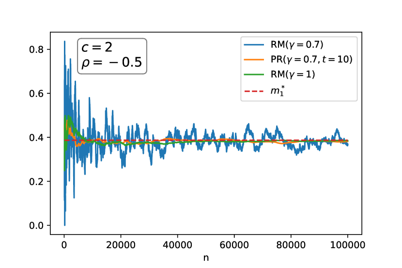
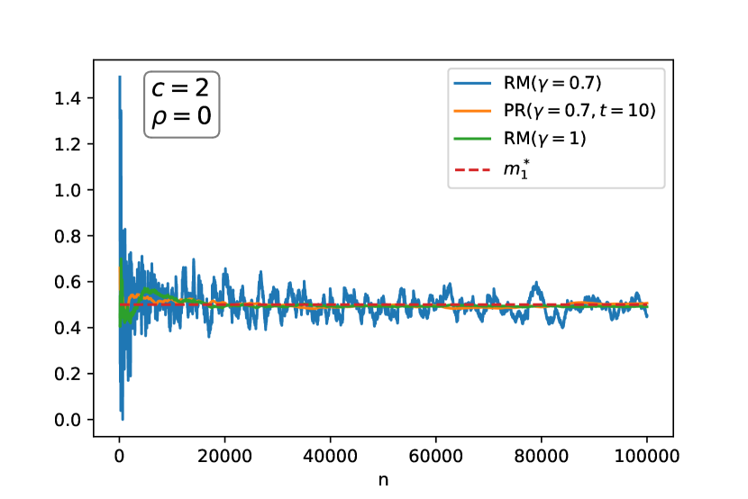
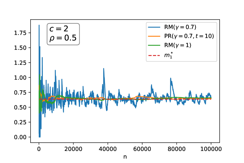
Figure 1: Consistency of RM/PR estimators with for different values of $\rho$.

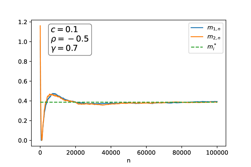
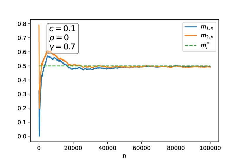
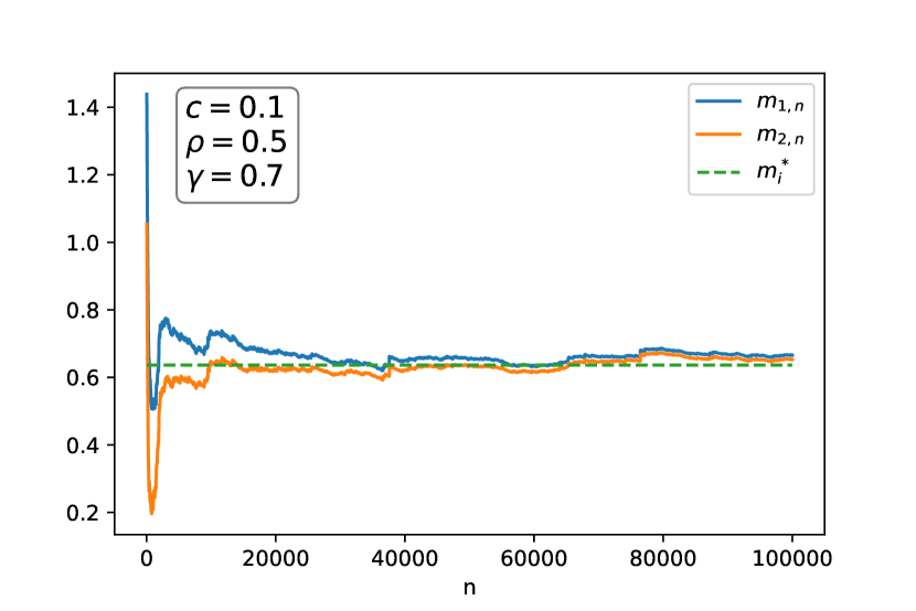
Figure 2: Consistency of RM estimators with $c=0.1$ for different values of $\rho$.

Note that we can easily verify that all conditions in ($\mathcal{A}$_a.s.) and ($\mathcal{A}$_a.n.) hold. We can also verify thanks to the exact formula of $\Sigma^{*}$, that this matrix is positive definite for the different values of $\rho$ used. This is a condition needed in Theorem 2.7.
For any random estimator, constructing confidence intervals is important to assess the error in the estimation. For PR estimator, confidence interval can be obtained in one simulation run after estimating matrices $\Sigma^{*}$ and $A$ and hence the asymptotic variance matrix $V$. Figure 3 shows the convergence, in the case $\rho=0$, of the estimator of $V_{n}=A_{n}^{-1}\Sigma_{n}(A_{n}^{-1})^{\intercal}$ where $A_{n}$ and $\Sigma_{n}$ are as introduced in Proposition 2.9.

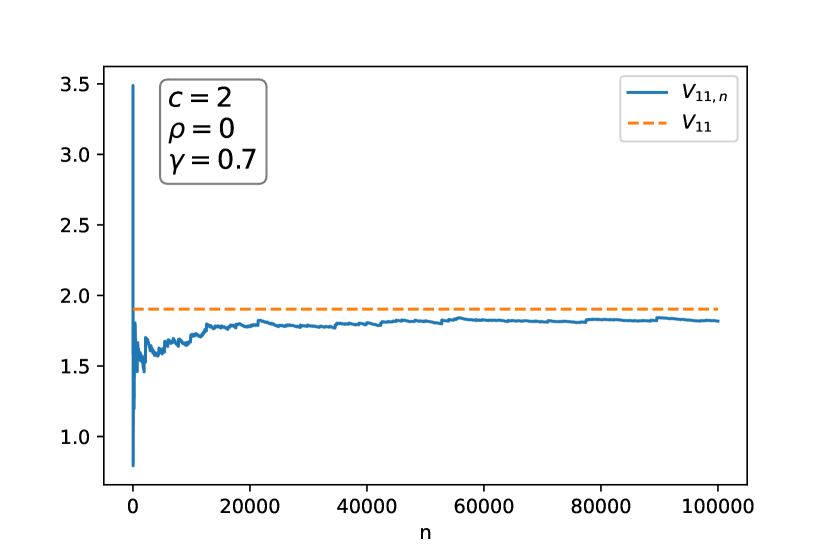
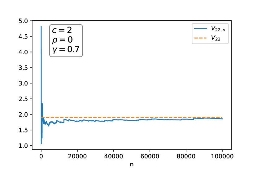
Figure 3: Convergence of the estimator $V_{n}$.

In the following table, we give the estimated confidence interval for PR estimator with a confidence coefficient of $95\%$:

Table 2: Confidence intervals for PR estimators.

$\rho$	CI for $m_{1}^{*}$	CI for $m_{2}^{*}$
$-0.5$	$[0.3772,0.4047]$	$[0.3679,0.3949]$
$0$	$[0.4962,0.5259]$	$[0.4912,0.5213]$
$0.5$	$[0.6194,0.6629]$	$[0.6203,0.6665]$

As for RM estimators, it is difficult to estimate the asymptotic covariance matrix due to its complexity. In order to visualize the normal behaviour of these estimators, we give the empirical probability density function (EPDF) in both cases $\gamma=1$ and $\gamma=0.7$. To this end, we use again a number of steps $n=100000$ and we repeat the procedure $N=10000$ times. We restrict our attention to the case $\rho=0$. Figure 4 shows that $D_{n,i}=\sqrt{n^{\gamma}}(m_{n,i}-m_{i}^{*}),i\in\{1,2\}$ are very close to a normal distribution.

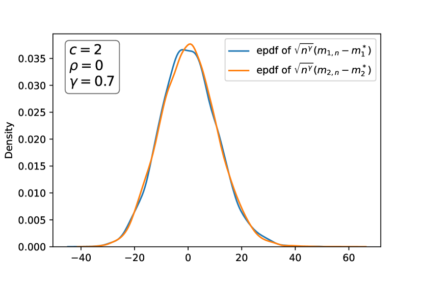
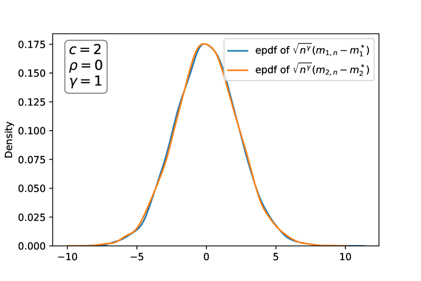
Figure 4: Empirical cumulative density function of $m_{n}-m^{*}$.

In order to appreciate the quality of convergence of RM estimators, we also give the empirical cumulative density function (ECDF) of the error $m_{n}-m^{*}$.

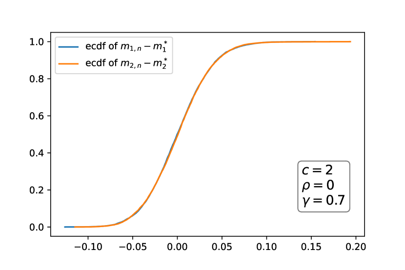
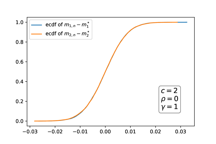
Figure 5: Empirical cumulative density function of $m_{n}-m^{*}$.

From the two figures above, the width of the $90\%$ confidence interval of the RM estimator for the case $\gamma=0.7$ is approximately $8\%$ and for the case $\gamma=1$ is roughly $2\%$.

3.2 Second example

As a second example, we will consider consider the following loss function used in Armenti et al. (2018):

$$l(x_{1},...,x_{d})=\sum_{i=1}^{d}x_{i}+\frac{1}{2}\sum_{i=1}^{d}(x_{i}^{+})^{2}+\alpha\sum_{i<j}x_{i}^{+}x_{j}^{+}.$$

3.2.1 First case: Gaussian distribution and $d=2$

We start by a simple case where we fix $d=2$ and use standard two dimensional Gaussian distribution for the loss vector $X$. We take $K=[0,2]^{3}$, $n=10^{5}$, $t=10$, $\alpha=1$ and $c=6$. Again, we compare RM and PR estimators for different values of $\rho$. The following figure 6 allows us to draw the same conclusions as in the previous example: RM estimator with $\gamma=1$ and PR estimator are better than RM estimator with $\gamma=0.7$. RM estimator with $\gamma=0.7$ is noisy and one can remediate to this by choosing a smaller value of $c$ as we did in the first example.

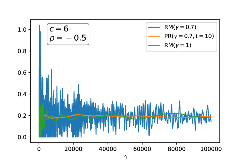
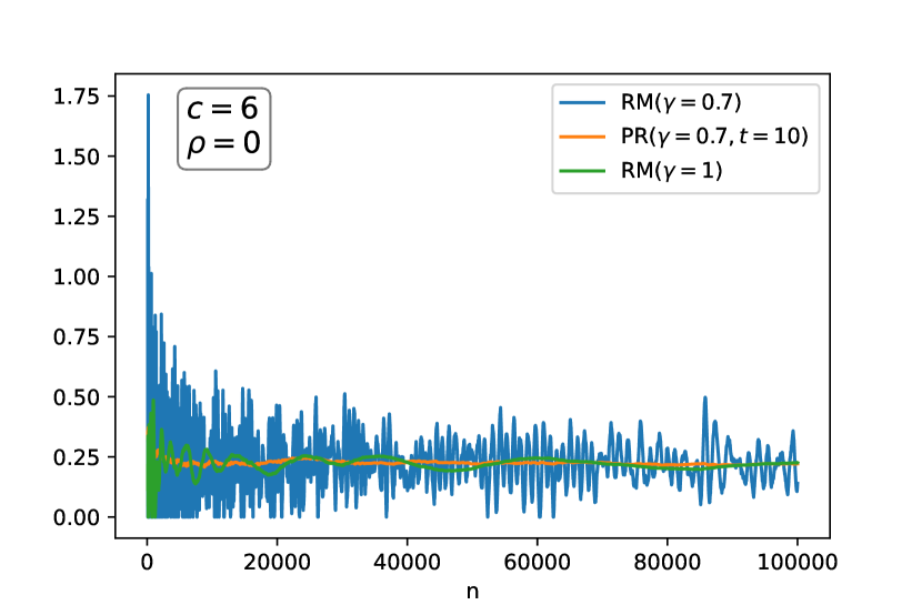
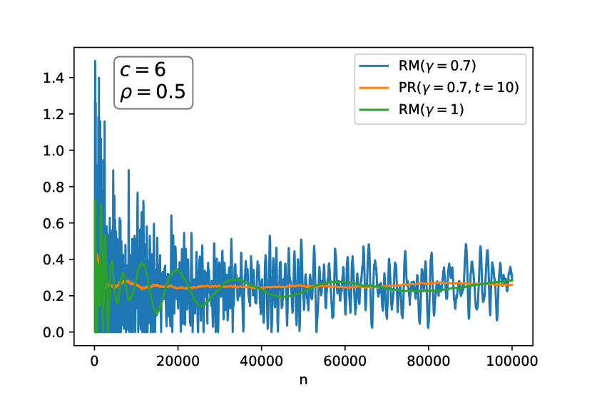
Figure 6: Consistency of RM/PR estimators with for different values of $\rho$.

In order to assess the accuracy of our PR estimator, we give the confidence interval with a $95\%$ confidence coefficient, using the estimators of Proposition 2.9.

Table 3: Confidence intervals for PR estimators.

$\rho$	$m_{1}^{*}=m_{2}^{*}$	CI for $m_{1}^{*}$	CI for $m_{2}^{*}$
$-0.5$	$0.188$	$[0.1790,0.2089]$	$[0.1746,0.2045]$
$0$	$0.21$	$[0.1963,0.2303]$	$[0.2044,0.2385]$
$0.5$	$0.25$	$[0.2415,0.2769]$	$[0.2424,0.2777]$

For RM estimator, we plotted the EPDF of $D_{n,i},i\in\{1,2\}$ as well as the ECDF of the error $m_{n}-m^{*}$ for the case $\rho=0$ and $\gamma=1$. These figures shows that the length of the confidence interval of 90% in the case $\gamma=0.7$ is much higher that in the case $\gamma=1$ (approx $0.2$ against $0.04$).

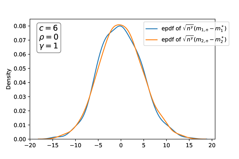
Figure 7: Empirical cumulative density function of $m_{n}-m^{*}$.

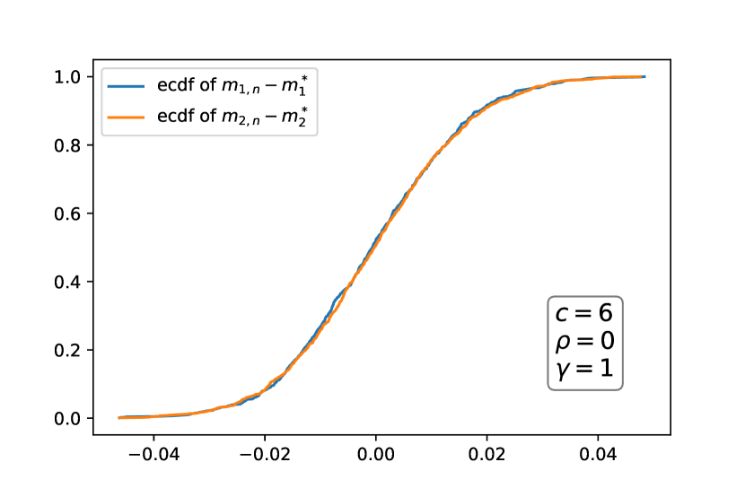
Figure 8: Empirical cumulative density function of $m_{n}-m^{*}$.

3.2.2 Second case: Compound Poisson Distribution and higher dimensions

In this section, we propose to use compound Poisson processes to model the loss vector $X$. The scope of application of compound Poisson processes is very wide. It ranges from statistical physics and biology to financial mathematics. In biology, they are used to study dynamics of populations. In the modern financial modeling, compound Poisson processes are used to describe dynamics of risk factors such as interest rates (see for instance Li et al. (2017)), foreign exchange rates and option pricing (see Jaimungal and Wang (2006)). In actuarial science, compound processes are extensively used to model claims sizes and to compute the ruin probability, i.e. the probability that the initial reserves increased by premiums received from clients and decreased by their claims, drops below zero.
More precisely, given a final time $T$, we consider a multivariate Poisson random vector $N^{T}=(N_{1}^{T},...,N_{d}^{T})$, where each $N_{i}^{T}\sim\mathcal{P}(\lambda_{i}T)$ and the loss corresponding to the $i^{\mathrm{th}}$ component is $X_{i}=\sum_{k=1}^{N_{i}^{T}}G_{i}^{k}$ and $(G_{i}^{k})_{k}$ is an i.i.d sequence representing the jump sizes and independent of $N_{i}^{T}$. We will take two examples for the distribution of the jumps sizes: One with a Gaussian distribution and another one with an exponential one. The correlation between the different components of $X$ will be done through the correlations between components of $N^{T}$. In what follows, we detail the method of generating a multivariate Poisson random vector, $N=(N_{1},...,N_{d})$ with a vector of corresponding intensities $(\lambda_{1},...,\lambda_{d})$. To do so, we will use a method that is based on the Gaussian vectors. More precisely, denote $\eta=(\eta_{1},...,\eta_{d})$ to be a Gaussian random vector having a centered normal distribution with correlation matrix $R=(\rho_{kl})$ and $\Phi$ to be the standard normal cdf. Then, the random vector $\xi=(\Phi(\eta_{1}),...,\Phi(\eta_{d}))$ has a multivariate distribution with standard uniform marginal distributions. Let $P_{\lambda}(x)=\sum_{j=0}^{[x]}(\lambda^{j}/j!)e^{-\lambda}$ be the cdf of the Poisson distribution with parameter $\lambda$. Now, consider the vector $\zeta=(\zeta_{1},...,\zeta_{d})$ where $\zeta_{k}=P^{-1}_{\lambda_{k}}(\Phi(\eta_{k})),k=1,...,d$. $\zeta$ has therefore Poisson marginal distributions with intensities $(\lambda_{1},...,\lambda_{d})$. We can express the correlation coefficient $\rho_{kl}^{*}=\mathrm{corr}(\zeta_{k},\zeta_{l})$ as a function of $\rho_{kl}=\mathrm{corr}(\eta_{k},\eta_{l})$:

$$\rho_{kl}^{*} =\frac{E(\zeta_{k}\zeta_{l})-E(\zeta_{k})E(\zeta_{l})}{\sigma(\zeta_{k})\sigma(\zeta_{l})}$$

$$=\frac{E(\zeta_{k}\zeta_{l})-\lambda_{k}\lambda_{l}}{\sqrt{\lambda_{k}\lambda_{l}}}.$$

We need to express the expectation $E(\zeta_{k}\zeta_{l})$ as a function of $\rho_{kl}$. We have:

$$E(\zeta_{k}\zeta_{l}) =E\left[P^{-1}_{\lambda_{k}}(\Phi(\eta_{k}))P^{-1}_{\lambda_{l}}(\Phi(\eta_{l}))\right]$$

$$=\sum_{m=1}^{\infty}\sum_{n=1}^{\infty}mn\leavevmode\nobreak\ P(\zeta_{k}=m,\zeta_{l}=n)$$

$$=\sum_{m=1}^{\infty}\sum_{n=1}^{\infty}mn\leavevmode\nobreak\ P(u_{m-1}^{k}\leq\Phi(\eta_{k})\leq u_{m}^{k},u_{n-1}^{l}\leq\Phi(\eta_{l})\leq u_{n}^{l}),$$

where $u_{j}^{i}=P_{\lambda_{i}}(j),i,j=1,...,d$. It remains to explicit the probabilities in the last equality. If we denote $\Phi_{2}(\cdot,\cdot,\rho_{kl})$ the bivariate Normal distribution function, we get finally that,

$$Z_{mn}(\rho_{kl}) \vcentcolon=P(u_{m-1}^{k}\leq\Phi(\eta_{k})\leq u_{m}^{k},u_{n-1}^{l}\leq\Phi(\eta_{l})\leq u_{n}^{l})$$

$$=\Phi_{2}(A_{m}^{k},B_{n}^{l},\rho_{kl})-\Phi_{2}(A_{m-1}^{k},B_{n}^{l},\rho_{kl})-\Phi_{2}(A_{m}^{k},B_{n-1}^{l},\rho_{kl})+\Phi_{2}(A_{m-1}^{k},B_{n-1}^{l},\rho_{kl})$$

where $A_{m}^{k}=\Phi^{-1}(P_{\lambda_{k}}(m))$ and $B_{n}^{l}=\Phi^{-1}(P_{\lambda_{l}}(n))$. As a conclusion, we obtain,

$$\sum_{m=1}^{\infty}\sum_{n=1}^{\infty}mnZ_{mn}(\rho_{kl})=\lambda_{k}\lambda_{l}+\rho_{kl}^{*}\sqrt{\lambda_{k}\lambda_{l}}.$$ (3.4)

The equation (3.4) gives an implicit relation between $\rho_{kl}^{*}$ and $\rho_{kl}$. It also involves two infinite sums which makes it hard to solve. In practice, one needs to truncate this sum and choose some appropriate upper-limits $M^{*}$ and $N^{*}$. We are then able to compute the elements of the correlation matrix $\rho$ of the Gaussian vector given the correlation matrix $\rho^{*}$ of the vector $N$. However, there is a problem of sufficient conditions for a given positive semi-definite matrix to be a correlation matrix of a multivariate Poisson random vector. This issue is tackled in Griffiths et al. (1979) where it is shown that each $\rho_{kl}^{*}$ has to be in a certain range,

$$-1<\rho_{kl}^{\min}\leq\rho_{kl}^{*}\leq\rho_{kl}^{\max}\leq 1.$$ (3.5)

Input: $(\lambda_{i})_{i=1,...,d}$, $(\sigma_{i})_{i=1,...,d}$, $T$ , and $\rho^{*}$ correlation matrix of $N_{T}$;

Ensure: For each $k>l$, $\rho_{kl}^{*}$ verifies the inequality in (3.5);

1 Solve the equation (3.4) to find $\rho$ the correlation of the Gaussian vector $\eta=(\eta_{1},...,\eta_{d})$;

2 Generate a sample of Gaussian vector $\eta$ with correlation matrix $\rho$ and for $i=1,...,d$;

3 for $i=1,...,d$ do

4       Set $N_{i}^{T}=P^{-1}_{\lambda_{i}T}(\Phi(\eta_{i}))$;

5       Generate a i.i.d sample of $G_{i}^{k}$ of size $N_{i}^{T}$;

6       Set $X_{i}=\sum_{k=1}G_{i}^{k}$.

Output: X;

Algorithm 1 Algorithm for generating a sample of $X$ with Compound Poisson Distribution

The following figure shows the covariance matrix for the loss vector $X$ of dimension $d=10$ obtained by generating a random correlation matrix $(\rho_{kl})$ and using a Gaussian distribution for the jump sizes, i.e. $G_{i}^{k}\sim\mathcal{N}(1,1)$. The intensity vector was taken uniformly in $[1,3]^{10}$.

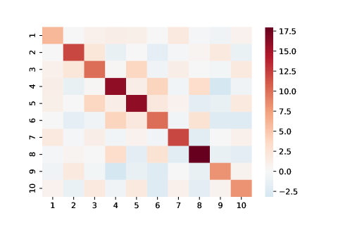
Figure 9: Correlation matrix of the vector loss $X$ with Gaussian jump sizes with means and variances equal to $1$.

Setting $K=[-20,20]^{10}\times[0,20]$, the averaging parameter $t=10$ and $c=6$, $\gamma=0.7$ and the number of steps $n=100000$, we obtain the following optimal allocations for both cases $\alpha=0$ and $\alpha=1$.

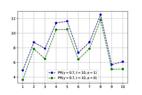
Figure 10: PR estimators for optimal allocations.

The above figure shows that there are components with the same optimal allocations for the case $\alpha=0$. This is something we expect to see, since with $\alpha=0$, correlations between components are not involved, so components with the same variance should have the same optimal allocations. This is the case for components $4-5$ and components $9-10$. However, once $\alpha$ is taken non null, we see that the same components have no longer the same optimal allocations. For instance, component $10$ has higher optimal allocation than $9$ when $\alpha=1$. This could be explained by the fact that component $10$ is more correlated with other components that have high variances, such as components $4$ and $5$, than component $9$. We now consider an exponential distribution for jump sizes as a second example, i.e. $G_{i}^{k}\sim\mathcal{E}(a_{i})$. The parameters $a_{i}$ were generated randomly in $[0.2,1.2]$. As for the other paramaters in this example, we took again $K=[-20,20]^{10}\times[0,20]$, $c=6$, $t=10$ and $\gamma=0.7$. Covariance matrix of the loss vector $X$ in this case and estimators of the optimal allocations obtained through PR algorithms with a number of steps $n=100000$ together with corresponding confidence intervals are given in the following figures.

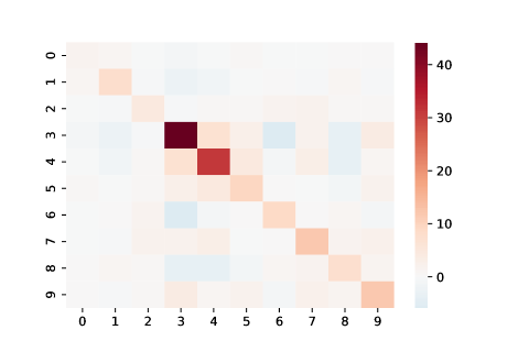
Figure 11: Correlation matrix of the vector loss $X$ with exponential distribution for the law of jump sizes.

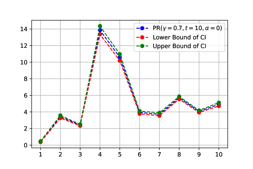
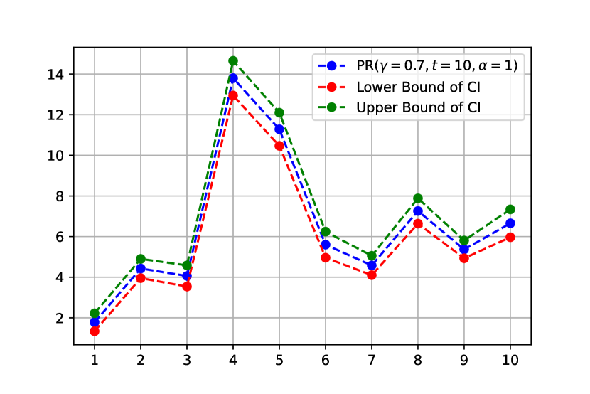
Figure 12: PR estimators for optimal allocations together with bounds of CI.

4 Appendix

4.1 ODE method and related concepts

Suppose we want to find the zeros of a function $h$. If we had a closed formula for $h$, under some classical conditions, we could use the following algorithm that ensures that at each step, we are going in the right direction: $Z_{n+1}=Z_{n}\pm\gamma_{n}h(Z_{n})$, where $(\gamma_{n})$ could be a constant sequence or decreasing toward $0$. However, if we do not have access to $h$, but only to random estimates $Y_{n}$ that are close to $h$ on average, then we could replace $h(Z_{n})$ by $Y_{n}$: $Z_{n+1}=Z_{n}+\gamma_{n}Y_{n}$. This is typically the case when $h$ is expressed as an expectation: $h(z)=E[H(X,z)]$ with $X$ is a random variable. An estimate of $h$ at step $n+1$, given all the $(Z_{i})_{i=0,..,n}$, is $Y_{n}=H(X_{n+1},Z_{n})$, where $X_{n+1}$ is a random variable that haves the same law as $X$. Then we could write the algorithm as:

$$Z_{n+1}=Z_{n}+\gamma_{n}H(X_{n+1},Z_{n}).$$ (4.1)

If we denote by $(\mathcal{F}_{n})$ the following filtration:

$$\mathcal{F}_{n}=\sigma(Z_{0},X_{i},i\leq n),$$

and rewrite:

$$Y_{n}=h(Z_{n})+\delta M_{n},$$

where $\delta M_{n}=Y_{n}-h(Z_{n})$. Observe that $h(Z_{n})=E[Y_{n}|\mathcal{F}_{n}]$ implies that $\delta M_{n}$ is a martingale difference sequence. Therefore, another way to write the (4.1) is as the following:

$$Z_{n+1}=Z_{n}+\gamma_{n}h(Z_{n})+\gamma_{n}\delta M_{n}.$$

The algorithm (4.1) is the regular Robbins-Monro (RM) procedure with mean function $h$. In order, to obtain a.s. convergence of the algorithm toward the $z^{*}$, one crucial condition among others, is the sublinearity of $h$, which is very constraining on the type of functions $h$ we can use. Consequently, we will drop the classical version of RM and will adopt the ordinary differential equation (ODE) point of view which offers more flexibility. The ODE method has its own drawbacks: it requires the sequence $(Z_{n})_{n\geq 1}$ to be in a compact set $K$ for non-explosion reasons. Still, this is not very constraining: In fact, each time $Z_{n}$ goes out of $K$, we will replace it by the closest point to $Z_{n}$ in $K$, using projection. In general, the behaviour of the algorithm (4.1) is determined by that of the associated ODE $\dot{z}=h(z)$. In what follows, we recall some stability concepts of ODEs that we have used in the article.

4.1.1 Concepts of stability of an ODE

As we have seen in the previous section, to study the behaviour of the sequence $(Z_{n})$, we need to study the behaviour of the associated ODE. In this section, we recall some key concepts of the stability of an ODE $\dot{z}=h(z)$. We start by giving the definition of an equilibrium point for the ODE.

Definition 4.1.

A state $z^{*}$ is an equilibrium of the ODE if $h(z^{*})=0$. In other words, this means that once $z(t)$ is equal to $z^{*}$ it remains equal to $z^{*}$ for all future times.

To describe the behaviour of the system around the equilibrium, a number of stability concepts are needed. Let us first introduce the basic concepts of stability. To alleviate the notations, we will take $0$ as an equilibrium state.

Definition 4.2.

The equilibrium $z^{*}=0$ is said to be stable, if for any $R>0$, there exists $r>0$ such that if $||z(0)||<r$, then $||z(t)||<R$ for all $t\geq 0$. Otherwise, the equilibrium is unstable.

Essentially, this means, the system can be kept arbitrarily close to the origin by starting sufficiently close to it. This is also know as Lyapunov stability. In some applications, Lyapunov stability is not enough: we not only want the system to remain in a certain range but we also want it to converge to the equilibrium. This behaviour is captured by the concept of asymptotic stability.

Definition 4.3.

An equilibrium point $z^{*}=0$ is asymptotically stable if it is stable, and if in addition, there exists some $r>0$ such that $||z(0)||<r$ implies that $z(t)\rightarrow 0$ as $t\rightarrow\infty$. The ball $B_{r}$ is called a domain of attraction of the equilibrium point.

The above definitions are formulated to characterize the local behaviour of the system, i.e., how the state evolves after starting near the equilibrium point. Local properties tell little about how the system will behave when the initial state is some distance away from the equilibrium. Global concepts are required for this purpose.

Definition 4.4.

If asymptotic stability holds for all initial states, the equilibrium is said to be globally asymptotically stable.

In the case of a linear system, i.e. described by $\dot{z}=Az$, where A is a $\mathbb{R}^{d}\times\mathbb{R}^{d}$ non-singular matrix, the solution is given by: $\forall t\geq 0,z(t)=z(0)\exp(tA)$. Therefore, the stability behaviour of the equilibrium point $z^{*}=0$ is stated by the eigenvalues of $A$. More precisely, the equilibrium point $z^{*}=0$ is globally asymptotically stable if and only if all eigenvalues of A have negative real parts. Moreover, if at least one eigenvalue of A has positive real part, then the equilibrium is unstable.
For nonlinear systems, Lyapunov’s linearization method states that a nonlinear system should behave similarly to its linearized approximation locally around the equilibrium. For instance, consider the system $\dot{z}=h(z)$ where $h:\mathbb{R}^{d}\mapsto\mathbb{R}^{d}$ is supposed to be continuously differentiable. Then, the system dynamics can be rewritten as:

$$\dot{z}=\left.\frac{\partial h}{\partial z}\right|_{z=0}z+h_{h.o.t}(z),$$

where $h_{h.o.t}$ stands for higher-order terms in $z$. Let us denote $A$ the Jacobian matrix of $h$ at $0$, $A=\left.\frac{\partial h}{\partial z}\right|_{z=0}$. Then, the system $\dot{z}=Az$ is called the linearization of the original system at the equilibrium point $0$. The following result (see Theorem 3.1 in Slotine and Li (1991)) establishes the relationship between the stability of the linear system and that of the original nonlinear system.

Theorem 4.5 (Theorem 3.1 in Slotine and Li (1991)).

• If all eigenvalues of A, the Jacobian matrix at $0$, have negative real parts, then the equilibrium point is asymptotically stable for actual nonlinear system.

• If at least one eigenvalue of A has positive real part, then the equilibrium is unstable for the nonlinear system.

The linearization method tells little about the global behaviour of stability of nonlinear systems. This motivates a deeper approach, known as Lyapunov’s direct method.

4.1.2 Lyapunov’s Direct Method

The intuition behind Lyapunov’s direct method is a mathematical extension of a fundamental physical observation: if the total energy of a mechanical or electrical system is continuously dissipated, then the system must eventually settle down to an equilibrium point. The basic procedure of Lyapunov is to generate an energy-like scalar function for the system and examine the time variation of that scalar function. This way, we may draw conclusions on the stability of differential equations without using the difficult stability definitions or requiring explicit knowledge of solutions.
The first property that need to be verified by this scalar function is positive definiteness.

Definition 4.6.

A scalar continuous function $V(z)$ is said to be locally positive definite if $V(0)=0$ and in around $0$, we have, $z\neq 0\Rightarrow V(z)>0$.
If the above property holds over the whole state space, then $V(z)$ is said to be globally positive definite.

The above definition implies that the function $V$ has a unique minimum at the origin $0$. Actually, given any function having a unique minimum point in a certain ball, we can construct a locally positive definite function by simply adding a constant to that function.
Next, we define the “derivative of V” with respect to time along the system trajectory. Assuming that $V$ is differentiable, this derivative is defined as:

$$\dot{V}(z)=\frac{dV(z)}{dt}=\nabla V,\dot{z}=\nabla V\cdot h(z).$$

Definition 4.7.

Let $V$ be a positive definite function and continuously differentiable. If its time derivative along any state trajectory is negative semi-definite, i.e.,

$$\dot{V}(z)=\nabla V_{z}\cdot h(z)\leq 0,\leavevmode\nobreak\ \leavevmode\nobreak\ \forall z,$$

then $V$ is said to be a Lyapunov function for the system.

4.1.3 Equilibrium Point Theorems

The relations between Lyapunov functions and the stability of systems are made precise in a number of theorems in Lyapunov’s direct method. Such theorems usually have local and global versions. The local versions are concerned with stability properties in the neighborhood of equilibrium point and usually a locally positive definite function. The next theorem (see Theorem 3.2 in Slotine and Li (1991)) gives a precise relation between Lyapunov function and stability.

Theorem 4.8 (Theorem 3.2 in Slotine and Li (1991)).

If, around $0$, there exists a scalar function $V$ with continuous derivative such that:

• $V$ is locally positive definite;

• $\dot{V}$ is locally negative semi-definite.

Then, the equilibrium point $0$ is stable. Moreover, if $\dot{V}$ is locally negative definite, then the stability is asymptotic;

The above theorem applies to the local analysis of stability. In order to assess the global asymptotic stability of a system, one might expect naturally that the local conditions in the above theorem has to be expanded to the whole state space. This is indeed necessary but not enough. An additional condition on the function $V$ has to be satisfied: $V$ must be coercive. We give more details in the following theorem (See Theorem 3.3 in Slotine and Li (1991)).

Theorem 4.9 (Theorem 3.3 in Slotine and Li (1991)).

Assume that there exists a scalar function $V$ continuously differentiable such that:

• $V$ is positive definite;

• $\dot{V}$ is negative definite;

• $V(z)\rightarrow\infty$ when $||z||\rightarrow\infty$.

Then, the equilibrium at origin is globally asymptotically stable.

Note that the coercive condition along with the negative definiteness of $\dot{V}$, implies, that given any initial condition $z_{0}$, the trajectories remain in the bounded region defined by $V(z)\leq V(z_{0})$.

4.1.4 Invariant Set Theorems

It is important to realize that the theorems in Lyapunov analysis are all sufficiency theorems. If for a particular choice of Lyapunov function candidate $V$, one of the conditions is not met, one cannot draw any conclusions on the stability of the system. In this kind of situations, fortunately, it is still possible to draw conclusions on asymptotic stability, with the help of the invariant set theorems introduced by La Salle. The central concept in these theorems is that of invariant set, a generalization of the concept of equilibrium point.

Definition 4.10.

Let $z(\cdot)$ be a solution of some ODE. A set $G$ is said to be an invariant set for this ODE if $z(0)\in G$ implies that $z(t)\in G,\leavevmode\nobreak\ \forall t\geq 0$.

For instance, the singleton $\{z^{*}\}$ where $z^{*}$ is an equilibrium point is an invariant set. Its domain of attraction is also an invariant set. One other trivial invariant set is the whole state-space, $\underset{z_{0}}{\cup}\{z(t),\leavevmode\nobreak\ t>0,\leavevmode\nobreak\ z(0)=z_{0}\}$. We first discuss the local version of the invariant set theorems as follows(see Theorem 3.4 of Slotine and Li (1991)).

Theorem 4.11 (Theorem 3.4 of Slotine and Li (1991)).

Consider the following ODE: $\dot{z}=h(z)$ and assume that $h$ is continuous. Let $V$ be a scalar function continuously differentiable such that:

• For some $l>0$, the region $\Omega_{l}\vcentcolon=\{z,V(z)<l\}$ is bounded.

• $\dot{V}(z)\leq 0$ for all $z\in\Omega_{l}$.

Let $R$ be the set of all points within $\Omega_{l}$ where $\dot{V}(z)=0$ and $M$ be the largest invariant set in $R$. Then, every solution $z(\cdot)$ originating in $\Omega_{l}$ tends to $M$ as $t\rightarrow\infty$.

Note that La Salle’s invariance theorem is only about convergence and not stability. The stability will be guaranteed once the condition of positive definiteness of $V$ is satisfied. However, La Salle’s theorem allow us to draw conclusions about the asymptotic behaviour of the system when Lyapunov’s direct method cannot be applied.

Corollary 4.12.

Let $V$ be a scalar function continuously differentiable and assume that in a certain neighborhood $\Omega$ of the origin:

• $V$ is locally positive definite;

• $\dot{V}$ is negative semi-definite;

• The largest invariant set in $R\vcentcolon=\{z\in\Omega,\dot{V}=0\}$ is reduced to $\{0\}$.

Then, the equilibrium point $0$ is asymptotically stable.

The above corollary replaces the negative definiteness condition on $\dot{V}$ in Lyapunov’s local asymptotic stability theorem by a negative semi-definiteness condition on $\dot{V}$, combined with a third condition on the trajectories within $R$.
The above invariant set theorem and its corollary can be easily extended to a global result by requiring again the radial unboundedness of the scalar function $V$.

4.2 Closed Formulas for the first example

In this subsection, we give the closed formulas obtained for the optimal risk allocations in the first example when $\alpha>0$. Recall that $d=2$ and

$$l(x_{1},x_{2})=\frac{1}{1+\alpha}\left[e^{\beta x_{1}}+e^{\beta x_{2}}+\alpha e^{\beta(x_{1}+x_{2})}\right]-\frac{\alpha+2}{\alpha+1}$$

and the loss vector $X$ is taken to follow a centered normal distribution with a covariance matrix $M=\begin{pmatrix}\sigma_{1}^{2}&\rho\sigma_{1}\sigma_{2}\\ \rho\sigma_{1}\sigma_{2}&\sigma_{2}^{2}\end{pmatrix}$. The optimal risk allocations $m_{i}^{*}$ are characterized by the first order conditions given in Theorem 1.6, i.e.

$$\left\{\begin{aligned} &\frac{\lambda^{*}}{1+\alpha}E\left[e^{\beta(X_{i}-m_{i}^{*})}+\alpha e^{\beta(X_{1}+X_{2}-m_{1}^{*}-m_{2}^{*})}\right]=1,\leavevmode\nobreak\ \leavevmode\nobreak\ i=1,2,\\ &\frac{1}{1+\alpha}E\left[e^{\beta(X_{1}-m_{1}^{*})}+e^{\beta(X_{2}-m_{2}^{*})}+\alpha e^{\beta(X_{1}+X_{2}-m_{1}^{*}-m_{2}^{*})}\right]-\frac{\alpha+2}{\alpha+1}=0.\end{aligned}\right.$$

The two first equations implies that $E[e^{\beta(X_{1}-m_{1}^{*})}]=E[e^{\beta(X_{2}-m_{2}^{*})}]$, which in turn gives that,

$$\frac{\beta\sigma_{1}^{2}}{2}-m_{1}^{*}=\frac{\beta\sigma_{2}^{2}}{2}-m_{2}^{*}.$$ (4.2)

The third equation gives $e^{\frac{\beta^{2}\sigma_{1}^{2}}{2}-\beta m_{1}^{*}}+e^{\frac{\beta^{2}\sigma_{2}^{2}}{2}-\beta m_{2}^{*}}+\alpha e^{\rho\beta^{2}\sigma_{1}\sigma_{2}+\frac{\beta^{2}}{2}(\sigma_{1}^{2}+\sigma_{2}^{2})-\beta(m_{1}^{*}+m_{2}^{*})}=2+\alpha$. Thanks to (4.2) and denoting $Q=e^{\frac{\beta^{2}\sigma_{i}^{2}}{2}-\beta m_{i}^{*}}$, we get that, $\alpha e^{\rho\beta^{2}\sigma_{1}\sigma_{2}}Q^{2}+2Q-(2+\alpha)=0$. Taking the positive solution of the last equation gives $Q=\frac{-1+\sqrt{1+\alpha(\alpha+2)e^{\rho\beta^{2}\sigma_{1}\sigma_{2}}}}{\alpha e^{\rho\beta^{2}\sigma_{1}\sigma_{2}}}$. Now, denoting by $\mathrm{SRC}=-\log(Q)$, we obtain that $m_{i}^{*}=\frac{\beta\sigma_{i}^{2}}{2}+\frac{1}{\beta}\mathrm{SRC}$.

References

- Armenti et al. (2018) Armenti, Y., Crépey, S., Drapeau, S., and Papapantoleon, A. (2018). Multivariate shortfall risk allocation and systemic risk. SIAM J. FINANCIAL MATH., 9(1):90–126.
- Artzner et al. (1999) Artzner, P., Delbaen, F., Eber, J.-M., and Heath, D. (1999). Coherent measures of risk. Mathematical Finance, 9(3):203–228.
- Bardou et al. (2009) Bardou, O., Frikha, N., and Pagès, G. (2009). Computing var and cvar using stochastic approximation and adaptive unconstrained importance sampling. Monte Carlo Methods and Applications, 15(3):173–210.
- Benveniste et al. (1990) Benveniste, A., Metivier, M., and Priouret, P. (1990). Adaptive Algorithms and Stochastic Approximations. Springer- Verlag, Berlin, 1 edition.
- Benzi et al. (2005) Benzi, M., Golub, G. H., and Liesen, J. (2005). Numerical solution of saddle point problems. Acta Numerica, 14:1–137.
- Biagini et al. (2019) Biagini, F., Fouque, J., Frittelli, M., and Meyer‐Brandis, T. (2019). A unified approach to systemic risk measures via acceptance sets. Mathematical Finance, 29(1):329–367.
- Chen et al. (2013) Chen, C., Iyengar, G., and Moallemi, C. C. (2013). An axiomatic approach to systemic risk. Management Science, 59(6):1373–1388.
- Duflo (1996) Duflo, M. (1996). Algorithmes stochastiques. Springer Berlin Heidelberg.
- Dunkel and Weber (2010) Dunkel, J. and Weber, S. (2010). Stochastic root finding and efficient estimation of convex risk measures. Operations Research, 58(5):1505–1521.
- Föllmer and Schied (2002) Föllmer, H. and Schied, A. (2002). Convex measures of risk and trading constraints. Finance and Stochastics, 6:429–447.
- Föllmer and Schied (2002) Föllmer, H. and Schied, A. (2002). Convex measures of risk and trading constraints. Finance and stochastics, 6(4):429–447.
- Frikha (2016) Frikha, N. (2016). Multi-level stochastic approximation algorithms. The Annals of Applied Probability, 26(2):933–985.
- Glasserman (2004) Glasserman, P. (2004). Monte Carlo Methods in Financial Engineering. Springer, New York, NY.
- Glasserman et al. (2008) Glasserman, P., Kang, W., and Shahabuddin, P. (2008). Fast simulation of multifactor portfolio credit risk. Operations Research, 56(5):1200–1217.
- Griffiths et al. (1979) Griffiths, R., Milne, R., and Wood, R. (1979). Aspects of correlation in bivariate poisson distributions and processes. Australian Journal of Statistics, 21(3):238–255.
- Hsieh and Glynn (2002) Hsieh, M.-h. and Glynn, P. W. (2002). Confidence regions for stochastic approximation algorithms. In Proceedings of the Winter Simulation Conference, volume 1, pages 370–376. IEEE.
- Jaimungal and Wang (2006) Jaimungal, S. and Wang, T. (2006). Catastrophe options with stochastic interest rates and compound poisson losses. Insurance: Mathematics and Economics, 38(3):469–483.
- Kleywegt et al. (2001) Kleywegt, A. J., Shapiro, a., and Homem de Mello, T. (2001). The sample average method for stochastic discrete optimization. SIAM Journal on Optimization, 12:479–502.
- Kushner and Sanvicente (1975) Kushner, H. J. and Sanvicente, E. (1975). Stochastic approximation for constrained systems with observation noise on the system and constraint. Automatica, 11:375–380.
- Kushner and Yang (1995) Kushner, H. J. and Yang, J. (1995). Stochastic approximation with averaging and feedback: Faster convergence. In Aström, K., Goodwin, G., and Kumar, P., editors, Adaptive Control, Filtering, and Signal Processing, pages 205–228. Springer, New York.
- Kushner and Yin (2003) Kushner, H. J. and Yin, G. (2003). Stochastic approximation and recursive algorithms and applications. Springer, New York, NY, 2 edition.
- Lemaire and Pagès (2010) Lemaire, V. and Pagès, G. (2010). Unconstrained recursive importance sampling. The Annals of Applied Probability, 20(3):1029–1067.
- Li et al. (2017) Li, S., Yin, C., Zhao, X., and Dai, H. (2017). Stochastic interest model based on compound poisson process and applications in actuarial science. Mathematical Problems in Engineering, 2017.
- Linderoth et al. (2006) Linderoth, J. T., Shapiro, a., and Wright, S. (2006). The empirical behavior of sampling methods for stochastic programming. Annals of Operations Research, 142:215–241.
- Ljung (1977) Ljung, L. (1977). Analysis of recursive stochastic algorithms. IEEE Transactions on Automatic Control, 22(4):551–575.
- Mak et al. (1999) Mak, W.-K., Morton, D. P., and Wood, R. K. (1999). Monte carlo bounding techniques for determining solution quality in stochastic programs. Operations Research Letters, 24:47–56.
- Polyak and Juditsky (1992) Polyak, B. T. and Juditsky, A. B. (1992). Acceleration of stochastic approximation by averaging. SIAM Journal on Control and Optimization, 30(4):838–855.
- Rao and Ren (1991) Rao, M. M. and Ren, Z. D. (1991). Theory of Orlicz Spaces. Marcel Dekker Inc. N.Y.
- Rockafellar (1970) Rockafellar, R. T. (1970). Convex Analysis. Princeton University Press, Princeton, NJ, princeton math. ser.28 edition.
- Rockafellar and Uryasev (2000) Rockafellar, R. T. and Uryasev, S. (2000). Optimization of conditional value-at-risk. Journal of Risk, 2(3):21–41.
- Ruppert (1991) Ruppert, D. (1991). Stochastic approximation. In Ghosh, B. K. and Sen, P., editors, Handbook of Sequential Analysis, pages 503–529. Dekker, New York.
- Shapiro et al. (2009) Shapiro, A., Dentcheva, D., and Ruszczynski, A. (2009). Lectures on Stochactic Programming: Modeling and Theory. SIAM.
- Shapiro and Nemirovski (2005) Shapiro, A. and Nemirovski, A. (2005). On complexity of stochastic programming problems. In Jeyakumar, V. and Rubinov, A., editors, Continuous Optimization, volume 99, pages 47–56. Springer, Boston, MA.
- Slotine and Li (1991) Slotine, J.-J. E. and Li, W. (1991). Applied Nonlinear Control, volume 199. Prentice hall Englewood Cliffs, NJ.
- Verweij et al. (2003a) Verweij, B., Ahmed, S., Kleywegt, A. J., Nemhauser, G., and Shapiro, A. (2003a). The sample average approximation method applied to stochastic routing problems: a computational study. Computational Optimization and Applications, 24:289–333.
- Verweij et al. (2003b) Verweij, B., Ahmed, S., Kleywegt, A. J., Nemhauser, G., and Shapiro, A. (2003b). The sample average approximation method applied to stochastic routing problems: a computational study. Computational Optimization and Applications, 24:289–333.