High-Dimensional Block Diagonal Covariance Structure Detection Using Singular Vectors

Abstract

The assumption of independent subvectors arises in many aspects of multivariate analysis. In most real-world applications, however, we lack prior knowledge about the number of subvectors and the specific variables within each subvector. Yet, testing all these combinations is not feasible. For example, for a data matrix containing 15 variables, there are already $1\,382\,958\,545$ possible combinations. Given that zero correlation is a necessary condition for independence, independent subvectors exhibit a block diagonal covariance matrix. This paper focuses on the detection of such block diagonal covariance structures in high-dimensional data and therefore also identifies uncorrelated subvectors. Our nonparametric approach exploits the fact that the structure of the covariance matrix is mirrored by the structure of its eigenvectors. However, the true block diagonal structure is masked by noise in the sample case. To address this problem, we propose to use sparse approximations of the sample eigenvectors to reveal the sparse structure of the population eigenvectors. Notably, the right singular vectors of a data matrix with an overall mean of zero are identical to the sample eigenvectors of its covariance matrix. Using sparse approximations of these singular vectors instead of the eigenvectors makes the estimation of the covariance matrix obsolete. We demonstrate the performance of our method through simulations and provide real data examples. Supplementary materials for this article are available online.

Keywords: Block diagonal covariance structure; High dimension; Independence test; $p>n$; Singular value decomposition; Variable selection

1 Introduction

Let $\bm{\Sigma}$ be the population covariance matrix of a $p$-dimensional random vector. Estimating and testing the structure of $\bm{\Sigma}$ and $\bm{\Sigma}^{-1}$ is important in numerous real-world applications. However, in high-dimensional contexts where the number of variables exceeds the number of observations, estimating and testing become challenging. Such scenarios arise, for example, in the analysis of DNA microarray gene expressions or in the detection of block diagonal structures prior to network inference for Gaussian graphical models (see, e.g., Fan and Li (2006), Tan et al. (2015), and related references). Consequently, there is a considerable interest in testing covariance matrices of high-dimensional data for a block diagonal structure. The objectives of these procedures can be categorized into two primary areas:

1. Tests for mutually uncorrelated random variables, specifically, testing for a diagonal covariance structure $\bm{\Sigma}=\operatorname{diag}(\sigma_{1}^{2},\ldots,\sigma_{p}^{2})$ with unknown but finite positive constants $\sigma_{1}^{2},\ldots,\sigma_{p}^{2}$ on the diagonal.

2. Testing for uncorrelated subvectors, i.e., assessing if the covariance matrix exhibits a block diagonal structure $\bm{\Sigma}=\operatorname{diag}(\bm{\Sigma}_{1},\ldots,\bm{\Sigma}_{b})$.

When testing the hypothesis $\bm{\Sigma}=\operatorname{diag}(\sigma_{1}^{2},\ldots,\sigma_{p}^{2})$, Bai et al. (2009) and Jiang and Yang (2013) extended classical likelihood ratio tests to the high-dimensional context. Alternative methods are based on the distance between the sample covariance matrix and the diagonal matrix $\operatorname{diag}(\sigma_{1}^{2},\ldots,\sigma_{p}^{2})$. Contributions in this category include Ledoit and Wolf (2002), Birke and Dette (2005), Fisher et al. (2010), and Chen et al. (2010). Furthermore, Johnstone (2001, 2008) used the distributional properties of the largest eigenvalue of the sample covariance matrix to construct hypothesis tests for sphericity. In addition, approaches for $\mathcal{L}_{2}$-type test statistics have been explored (see, e.g., Schott (2005) and Leung and Drton (2018)).

In the context of testing the hypothesis $\bm{\Sigma}=\operatorname{diag}(\bm{\Sigma}_{1},\ldots,\bm{\Sigma}_{b})$, Jiang and Yang (2013) also extended the likelihood ratio approach for this hypothesis to high-dimensional data, and Jiang et al. (2013) proposed a corrected likelihood ratio test and a large-dimensional trace criterion. Among others, Srivastava and Reid (2012), Hyodo et al. (2015), Yata and Aoshima (2016), and Yamada et al. (2017) used empirical distances between the covariance matrix and its block diagonal form to derive test statistics. In addition, Bao et al. (2017) extended the Schott type test (Schott, 2005) to test for independence of random vectors, and Székely and Rizzo (2013) provided a test based on an extension of the distance correlation (Székely et al., 2007) to high-dimensional contexts.

In most applications, however, we lack prior knowledge about the number of blocks and the specific variables within each block. The number of possible distinct combinations of $p$ random variables into different blocks of unknown size can be calculated using the Bell number. For example, with $p=15$ variables, there are already around $1\,382\,958\,545$ possible combinations. Yet, testing all these combinations in high-dimensional contexts is not feasible due to the increasing risk of test errors.

Therefore, methods for detecting block diagonal structures of covariance matrices are needed. So far, Pavlenko et al. (2012), Tan et al. (2015), and Devijver and Gallopin (2018) have proposed approaches to address this problem. Pavlenko et al. (2012) obtained block sparsity by extending the graphical lasso (Friedman et al., 2007) which applies $\mathcal{L}_{1}$ regularization on the entries of the estimated covariance matrix. Tan et al. (2015) recognized that the first step of the graphical lasso involves single linkage hierarchical clustering of the variables. However, single linkage clustering can yield suboptimal results in finite-sample contexts. To address this limitation, they introduced the cluster graphical lasso, which uses alternative linkages than single linkage for clustering. Devijver and Gallopin (2018) took a different approach. To detect block diagonal structures, they select the best fitting model from a collection of multivariate distributions with block diagonal covariance matrices. This collection of models is generated through hard-thresholding of the sample covariance matrix.

In this article, we contribute a novel nonparametric approach for detecting block diagonal structures. We exploit that the structure of the right singular vectors of the mean-centered data matrix mirror the block diagonal structure of the covariance matrix. This mirroring feature allows us to uncover the structure of the data matrix effectively. In practice, however, sample noise in the data matrix masks the block diagonal structure, consequently masking also the sample singular vectors. We propose employing sparse singular vectors, named sparse loadings, to reveal the block diagonal structure. These sparse loadings are sparse approximations, i.e., have many zero values, of the sample singular vectors and can reflect the inherent structure of the population singular vectors. Their computation aligns with lasso-type regression, presenting a convenient pathway for employing the Bayesian information criterion to identify sparse loadings that represent the structure inherent in the population singular vectors.

The rest of this article is organized as follows: In Section 2, after introducing basic notations and definitions, we present the concept for block diagonal covariance matrix detection using singular vectors. We provide elaborate simulation studies in Section 3, and real data examples in Section 4. Section 5 contains the discussion.

2 Singular Vectors to Detect Block Diagonal Structure

2.1 Preliminaries and Basic Ideas

Let $\bm{X}\equiv(\bm{x}_{1},\ldots,\bm{x}_{p})\equiv(\bm{X}_{1},\ldots,\bm{X}_{b})$ denote an $n\times p$ matrix of data. $\bm{X}$ contains $n$ observations, $p$ variables, $n\times 1$ column vectors $\bm{x}_{1},\ldots,\bm{x}_{p}$, and is partitioned into $b$ distinct submatrices: $\bm{X}_{i}$ of dimension $n\times p_{i}$ for $i\in\{1,\ldots,b\}$ where $p=p_{1}+\ldots+p_{b}$. Each $\bm{X}_{i}$ is organized such that $\bm{X}_{1}=(\bm{x}_{1},\ldots,\bm{x}_{p_{1}})$ contains the first $p_{1}$ columns of $\bm{X}$, $\bm{X}_{2}$ contains the next $p_{2}$ columns of $\bm{X}$, and so forth. We assume the convenient ordering $\bm{X}\equiv(\bm{X}_{1},\ldots,\bm{X}_{b})^{\top}$ since this order can be obtained by using row permutation. The singular value decomposition (SVD) of the data matrix can be written as follows:

$$\bm{X}=\bm{U}\bm{D}\bm{V}^{\top},\;\bm{U}^{\top}\bm{U}=\bm{I}_{n},\;\bm{V}^{\top}\bm{V}=\bm{I}_{p},\;d_{1}\geq\ldots\geq d_{r}>0\,,$$

where $r\leq\min(n,p)$ is the rank of $\bm{X}$, and $\bm{U}=(\bm{u}_{1},\ldots,\bm{u}_{n})$ and $\bm{V}=(\bm{v}_{1},\ldots,\bm{v}_{p})$ are the left and right singular vectors respectively. Without loss of generality, assume that the overall mean of $\bm{X}$ is zero. This implies that the right singular vectors of the data matrix are the eigenvectors of the sample covariance matrix.

We assume that the population covariance matrix $\bm{\Sigma}$ follows a block diagonal structure:

$$\bm{\Sigma}\equiv\begin{pmatrix}\bm{\Sigma}_{1}&\bm{0}&\bm{0}\\ \bm{0}&\ddots&\bm{0}\\ \bm{0}&\bm{0}&\bm{\Sigma}_{b}\end{pmatrix}\,,$$

where $\bm{\Sigma}_{i}$ is the population covariance matrix corresponding to the submatrix $\bm{X}_{i}$ for $i\in\{1,\ldots,b\}$, and the population covariance between these submatrices is $\bm{0}$. In practice, we have only access to the sample covariance matrix of the observed data, which we denote by $\bm{S}$. The sample covariance matrix can be expressed by the population covariance matrix, perturbed by a noise matrix $\bm{\mathrm{E}}$,

$$\bm{S}\equiv\bm{\Sigma}+\bm{\mathrm{E}}\,,$$

which masks the block diagonal structure of $\bm{\Sigma}$.

Assume for now that $\bm{\mathrm{E}}=\bm{0}$ such that $\bm{S}$ exhibits the block diagonal structure of $\bm{\Sigma}$. It holds that the right singular vectors of $\bm{X}$ mirror the block diagonal structure of the covariance matrix:

Corollary 1.

$\bm{S}$ is a block diagonal matrix iff its eigenvectors (the right singular vectors of $\bm{X}$) exhibit the structure

$$\bm{V}\bm{P}_{\pi}=\begin{pmatrix}\bm{V}_{1}&\bm{0}&\bm{0}\\ \bm{0}&\ddots&\bm{0}\\ \bm{0}&\bm{0}&\bm{V}_{b}\end{pmatrix}\,,$$ (1)

where $\bm{V}_{i}$ are the eigenvectors of $\bm{S}_{i}$ (the right singular vectors of $\bm{X}_{i}$) for $i\in\{1,\ldots,b\}$, and $\bm{P}_{\pi}$ is a permutation matrix leading to a block diagonal structure.

Consequently, by analyzing the structure of the singular vectors, it is possible to identify the block diagonal pattern of $\bm{S}$ and thus detect the presence of uncorrelated submatrices.

We saw that the singular vectors exhibit a structure that mirrors the block diagonal structure when $\bm{\mathrm{E}}=\bm{0}$. Under more realistic conditions when $\bm{\mathrm{E}}\neq\bm{0}$, however, the singular vectors are also perturbed by $\bm{\mathrm{E}}$. Let $\lambda_{1}\geq\ldots\geq\lambda_{p}$ be the sample eigenvalues of $\bm{S}$, and $\tilde{\lambda}_{1}\geq\ldots\geq\tilde{\lambda}_{p}$ be the population eigenvalues with corresponding population eigenvectors $\tilde{\bm{v}}_{1},\ldots,\tilde{\bm{v}}_{p}$ of $\bm{\Sigma}$ that perfectly mirror its block diagonal structure. From the Davis-Kahan theorem (Yu et al., 2015; Bauer and Drabant, 2021), we can conclude that the distance between the population and sample eigenvectors is perturbed. For the purpose of completeness, we provide the corresponding result from Yu et al. (2015).

Corollary 2.

Let $\delta_{i}\equiv\min(\tilde{\lambda}_{i-1}-\tilde{\lambda}_{i},\tilde{\lambda}_{i}-\tilde{\lambda}_{i-1})$ be the eigengap of the eigenvalue $\tilde{\lambda}_{i}$, where $\tilde{\lambda}_{0}=\infty$ and $\tilde{\lambda}_{p+1}=-\infty$. If $\delta_{i}>0$ it holds that

$$\|\tilde{\bm{v}}_{i}-\bm{v}_{i}\|\leq\dfrac{2^{3/2}\|\bm{\mathrm{E}}\|_{\rm op}^{2}}{\delta_{i}}\,,$$

for $i\in\{1,\ldots,p\}$ where $\|\cdot\|_{\rm op}$ denotes the operator norm.

In this work, we provide a concept that identifies the block diagonal structure of the population covariance matrix using sample singular vectors of the data matrix $\bm{X}$ also in the presence of noise.

2.2 An Iterative Algorithm

In Corollary 1, we conclude that the singular vectors mirror the block diagonal shape of the covariance matrix $\bm{\Sigma}$. In the sample case, however, the block diagonal structure is masked by noise. As a result, the sample singular vectors are perturbed by $\bm{\mathrm{E}}$ (Corollary 2) and therefore do not perfectly mirror the block diagonal structure of $\bm{\Sigma}$.

To recover their unperturbed structure and thereby reveal the block diagonal structure of the population covariance matrix, we propose the use of sparse singular vectors. These so called sparse loadings are sparse approximations, i.e., having many zero entries, of the sample singular vectors. The intuition of using them is that by calculating sparse loadings, the zero elements of the population singular vectors, which may deviate from zero due to the perturbation $\bm{\mathrm{E}}$ in their estimated sample counterparts, are reset to their original zero values. Calculation of sparse loadings is a well-established area in the literature for which numerous approaches have been proposed (see, e.g., Zou et al. (2006), Shen and Huang (2008), Witten et al. (2009), Yang et al. (2014), and Gataric et al. (2020) among others). These methods typically employ a form of regularization, such as the $\mathcal{L}_{1}$-type lasso constraint (Tibshirani, 1996), the hard thresholding penalty (Donoho and Johnstone, 1994), or the smoothly clipped absolute deviation penalty (Fan and Li, 2001). We consider the former to obtain sparse loadings according to the following optimization problem:

$$\min\limits_{d,\bm{u},\bm{v}}\|\bm{X}-d\bm{u}\bm{v}^{\top}\|_{F}^{2}\;\;{\rm subject\;to}\;\;\|\bm{u}\|_{2}^{2}=1,\;\|\bm{v}\|_{2}^{2}=1,\;\|\bm{v}\|_{1}\leq\alpha\,,$$ (2)

which calculates the first sparse loading $\check{\bm{v}}_{1}$ with $\|\check{\bm{v}}_{1}\|_{2}^{2}=1$ and $\mathcal{L}_{1}$ imposing regularization parameter $\alpha$. Throughout this paper, $\|\bm{v}\|_{p}$ denotes the $\mathcal{L}_{p}$ norm for any vector $\bm{v}$. The remaining sparse loadings for $i>1$ can then be calculated iteratively. For this the data matrix $\bm{X}$ must be replaced by the residual matrices of the sequential matrix approximations.

However, the block diagonal structure can be revealed using only the first singular vector. The intuition is that the first singular vector mirrors one block which can then be omitted for further analysis. For example, assume without loss of generality that the first singular vector mirrors the first submatrix $\bm{X}_{1}$. After detection, we can proceed with the calculation of the first singular vector of the reduced data matrix $\bm{X}_{-1}\equiv(\bm{X}_{2},\ldots,\bm{X}_{b})$, omitting the first submatrix $\bm{X}_{1}$. This is done iteratively to find all submatrices one after the other.

When using sparse loadings in the practical implementation, the precision of block detection may be somewhat compromised. The first sparse loading partitions the data matrix into two submatrices: one determined by the non-zero loading components and the other by the zero-valued loading components. While these submatrices may not directly align with the actual population blocks, an recursive refinement process is employed to uncover the true underlying block structure. The steps for this recursive refinement are outlined in Algorithm 1, which illustrates the method for block detection using singular vectors (BD-SVD).

Algorithm 1 Procedure for BD-SVD

1:Input $n\times p$ data matrix $\bm{X}$ with centered columns.

2:Calculate the first sparse loading $\check{\bm{v}}_{1}$ with regularization parameter $\alpha$.

3:Check if $\check{\bm{v}}_{1}$ mirrors one or two blocks.

4:Repeat steps 1 to 2 for the respective subsamples corresponding to the blocks detected in step 2 until the sparse loading $\check{\bm{v}}_{1}$ no longer mirrors a more refined block diagonal structure. This means continuing until the first sparse loading for each subsample mirrors only one block, namely the subsample itself.

5:Output Detected structure $\bm{X}=(\bm{X}_{1},\ldots,\bm{X}_{b})$ with subsamples $\bm{X}_{1},\ldots,\bm{X}_{b}$ of the data matrix concluding that $\bm{\Sigma}=\operatorname{diag}(\bm{\Sigma}_{1},\ldots,\bm{\Sigma}_{b})$ exhibits a block diagonal structure.

2.3 Parameter Tuning

We treat the regularization $\alpha$ as tuning parameter in step 2 of Algorithm 1 and the sparse loading $\check{\bm{v}}_{1}\equiv\check{\bm{v}}_{1}(\alpha)$ depends on the sparsity induced by $\alpha$. Theoretically, we can increase sparsity by increasing $\alpha$ until $\check{\bm{v}}_{1}$ becomes the standard base vector, suggesting that all variable are mutually uncorrelated. However, imposing such extreme sparsity may not reflect the true underlying structure of the population covariance matrix. Therefore, there is a need to control the degree of regularization and strive for a reasonable level of sparsity. In this section, we propose an approach for tuning the parameter $\alpha$.

We formulate the computation of sparse loadings as a lasso regression problem. This formulation allows us to utilize the Bayesian information criterion (BIC) (Schwarz, 1978) for lasso regression to determine the parameter $\alpha$ that leads to the sparse loading $\check{\bm{v}}_{1}\equiv\check{\bm{v}}_{1}(\alpha)$ that best fits the covariance matrix. To begin with, we note that the computation of sparse loadings can be stated as a lasso regression problem.

Remark 1.

Assume that $\|\bm{v}\|_{2}^{2}=1$. The optimization problem from (2) can be formulated as

$$\min\limits_{d,\bm{u},\bm{v}}\|\bm{X}-d\bm{u}\bm{v}^{\top}\|_{F}^{2}+\lambda_{v}\|\bm{v}\|_{1}\,,$$

where $\lambda_{v}\geq 0$ is a regularization parameter. For a fixed $\bm{v}=\check{\bm{v}}$ with $\|\check{\bm{v}}\|_{2}^{2}=1$, its minimum is

$$\|\bm{X}-\check{\bm{u}}\check{\bm{v}}^{\top}\|_{F}^{2}+\lambda_{v}\|\check{\bm{v}}\|_{1}\,,$$ (3)

with $\check{\bm{u}}=\bm{X}\check{\bm{v}}$.

For the first sparse loading $\check{\bm{v}}_{1}$, we use the optimization problem outlined above. The unit length assumption holds without loss of generality, since we can always replace the sparse loading by $\check{\bm{v}}_{1}/\|\check{\bm{v}}_{1}\|_{2}^{2}$ without affecting the sparseness of its structure. When calculating $\check{\bm{v}}_{i}$ for $i>1$, the data matrix $\bm{X}$ needs to be replaced by the residual matrices of the sequential matrix approximations: $\bm{X}^{(i)}\equiv\bm{X}^{(i-1)}-\check{\bm{u}}_{i-1}\check{\bm{v}}_{i-1}^{\top}$ where $\check{\bm{u}}_{i-1}=\bm{X}^{(i-1)}\check{\bm{v}}_{i-1}$ and $\bm{X}^{(0)}\equiv\bm{X}$.

Now, we can adopt the BIC for lasso regression as a selection criteria. Let $\mathcal{S}\equiv\operatorname*{supp}(\check{\bm{v}}_{1})$ be the support of the sparse loading $\check{\bm{v}}_{1}$. We use $|\mathcal{S}|$ to denote the cardinality of the set $\mathcal{S}$, i.e. , the number of non-zero components in $\check{\bm{v}}_{1}$. Zou et al. (2007) showed that $|\mathcal{S}|$ is an unbiased estimate for the degree of freedom of the lasso fit, and propose that the BIC can be used to select the optimal number of non-zero coefficients. We apply this result to our objective of selecting the degree of sparsity by using the connection between the calculation of sparse loadings and regularized regression (Remark 1). In addition, we consider a high-dimensional BIC (HBIC) which also applies in high-dimensional contexts (Wang et al., 2009; Fan and Tang, 2012; Wang et al., 2013).

Remark 2.

Let ${\rm SSR}\equiv\|\bm{X}-\check{\bm{u}}_{1}\check{\bm{v}}_{1}^{\top}\|_{F}^{2}$ be the sum of squared residuals. The HBIC for the first sparse loading $\check{v}_{1}$ according to the lasso regularization problem (3) in Remark 1 is

$${\rm HBIC}\equiv\log\left(\dfrac{{\rm SSR}}{np}\right)+|\mathcal{S}|\dfrac{a_{np}}{np}\log(p)\,,$$ (4)

where $a_{np}$ is a positive sequence of numbers that diverges to infinity.

Wang et al. (2013) showed that if $p_{i}a_{np}\log(p)=o(np)$ for $i\in\{1,\ldots,b\}$, then HBIC identifies the true underlying model with probability approaching one under mild conditions. These conditions are also intended for scenarios in which the number of variables exceeds the number of observations in the data matrix, commonly referred to as the ”$p>n$” case. However, the lasso regularization we formulated always addresses a ”$p<n$” problem with $n_{\rm lasso}=np$ observations and $p_{\rm lasso}=p$ variables (online Appendix A.3), making it easier to meet the HBIC conditions. At the same time, meeting the conditions required for other criteria like the extended BIC (Chen and Chen, 2008) is a greater challenge due to the constructed ”$p<n$” case.

For parameter tuning, we compute $\check{\bm{v}}_{1}$ for $|\mathcal{S}|\in\{0,\ldots,p-1\}$ and select the optimal sparse loading with parameter $\alpha$ according to the HBIC in (4). The choice of $a_{np}=\log(np)^{2/3}\log\log(np)$ has proven successful in our experience.

2.4 Illustrative Example

In this section, we provide an illustrative example of BD-SVD. We generated a synthetic data matrix $\bm{X}=(\bm{x}_{1},\ldots,\bm{x}_{3000})=(\bm{X}_{1},\bm{X}_{2},\bm{X}_{3})$ comprising $n=500$ observations and $p=3000$ variables. These variables are partitioned into three equally sized blocks, resulting in $\bm{X}_{i}$ as $500\times 1000$ matrices for $i\in\{1,2,3\}$. The sample was drawn from an $N(\bm{0},\bm{\Sigma})$ distribution with population covariance matrix $\bm{\Sigma}=\operatorname{diag}(\bm{\Sigma}_{1},\bm{\Sigma}_{2},\bm{\Sigma}_{3})$ with $\bm{\Sigma}_{i}=(1-\omega_{i})\bm{I}_{1000}+2\omega_{i}\bm{1}_{1000}\bm{1}_{1000}^{\top}$ where $\omega_{i}$ is uniformly $U(0.1,0.3)$ distributed and $\bm{1}_{1000}$ is a vector of ones.

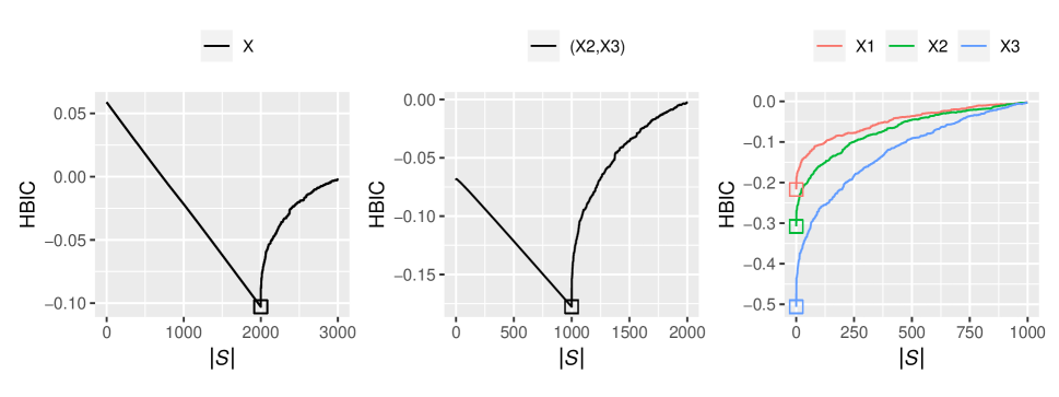
Figure 1: Illustration of block detection by BD-SVD for the data matrix $\bm{X}=(\bm{X}_{1},\bm{X}_{2},\bm{X}_{3})$ using HBIC from (4) for parameter tuning. In the initial step (left), $\bm{X}$ is split into two blocks: $\bm{X}_{1}$ and $(\bm{X}_{2},\bm{X}_{3})$, where the optimal number of non-zero components is $|\mathcal{S}|=2000$ according to HBIC, and $\mathcal{S}=\{1001,\ldots,3000\}$. With $|\mathcal{S}|=1000$ in the subsequent step (center), $(\bm{X}_{2},\bm{X}_{3})$ is further split into $\bm{X}_{2}$ and $\bm{X}_{3}$. The final structure has now been set. BD-SVD does not perform any further splits for $\bm{X}_{1}$, $\bm{X}_{2}$, or $\bm{X}_{3}$ (right), since $|\mathcal{S}|=0$ for all three matrices according to HBIC.

Figure 1 illustrates the steps of BD-SVD given in Algorithm 1 until all three blocks, and therefore the block diagonal structure of the population covariance matrix, are identified. For this example and throughout this work, we compute sparse loadings using the method of Shen and Huang (2008) in step 1 of Algorithm  1. Shen et al. (2013) established consistency of this method in high-dimensional and low sample size contexts. The implementation of the method is available in the irlba package (Baglama et al., 2022) within the statistical software R (R Core Team, 2022).

2.5 Number of Sparse Loadings

In Corollary 1, we conclude that the structure of a block diagonal covariance matrix is mirrored by all singular vectors. Therefore, it seems valid to choose all singular vectors ($k=p$) to identify the block diagonal structure of the covariance matrix. Further, the covariance matrix can be approximated by a reduced number of singular vectors, meaning that choosing a smaller number of vectors ($k<p$) but with $k>1$ to achieve a good approximation could be a good choice as well. The advantage is that we avoid calculating the first sparse loading $\check{\bm{v}}_{1}$ recursively until the block diagonal structure of the covariance is revealed, but rather calculate $\check{\bm{V}}=(\check{\bm{v}}_{1},\ldots,\check{\bm{v}}_{k})$ with $k>1$ that mirrors the true shape directly.

We recap (see, e.g., Eckart and Young (1936)) that for any $k\leq r$

$$\bm{S}^{(k)}\equiv\sum\limits_{i\in\{1,\ldots,k\}}\lambda_{i}\bm{v}_{i}\bm{v}_{i}^{\top}=\operatorname*{arg\,min}\limits_{\hat{\bm{S}}\,:\,\operatorname*{rank}(\hat{\bm{S}})\leq k}\|\bm{S}-\hat{\bm{S}}\|_{F}^{2}\;,$$

is the best rank-$k$ approximation to $\bm{S}$ in the sense of the squared Frobenius norm ($\|\cdot\|_{F}^{2}$). If we are able to reveal the block diagonal structure from $\bm{S}$ using all singular vectors (Corollary 1), it is reasonable that this is also possible using $k$ singular vectors of a low rank approximation $\bm{S}^{(k)}$ of $\bm{S}$ with $k<r$.

In Remark 1, we recapped calculation of $\check{\bm{v}}_{i}$ for $i\geq 1$. Tuning of the regularization parameter $\alpha$ using the HBIC can be done as follows.

Remark 3.

Let ${\rm SSR}(k)\equiv\sum_{i\in\{1,\ldots,k\}}\|\bm{X}^{(i)}-\check{\bm{u}}_{i}\check{\bm{v}}_{i}^{\top}\|_{F}^{2}$ and let $|\mathcal{S}_{i}|$ be the support of $\check{\bm{v}}_{i}$ such that $|\mathcal{S}(k)|\equiv\sum_{i\in\{1,\ldots,k\}}|\mathcal{S}_{i}|$ denotes the overall degree of sparsity. The HBIC for the first $k$ sparse loadings according to the lasso regularization problem in Remark 1 is

$${\rm HBIC}\equiv\log\left(\dfrac{{\rm SSR}(k)}{npk}\right)+|\mathcal{S}(k)|\dfrac{a_{npk}}{npk}\log(pk)\,.$$

Singular vectors corresponding to singular values with multiplicity greater than one, or those corresponding to singular values that are nearly equal to each other, are strongly masked in the sample case (Corollary 2). This poses a challenge in revealing their inherent structure and argues in favor of not choosing singular vectors corresponding to these singular values. With $k=1$ however, this concern is less likely to occur. In particular, spiked covariance models (Paul, 2007; Johnstone and Lu, 2009) which are frequently used to model high-dimensional phenomena, indicate that singular values outside the spikes are in close distance, which also argues in favor of not using all singular vectors.

3 Simulation Studies

In this section, we evaluate the performance of BD-SVD described in Section 2 with $k=1$. We simulate a data matrix containing $n$ observations from a $p$-multivariate normal distribution $N(\bm{0},\bm{\Sigma})$. BD-SVD is compared to three other approaches:

1. SHDJ and SHRR: In their recent work, Devijver and Gallopin (2018) demonstrated that their methods (SHDJ and SHRR) outperformed existing ones. Therefore, these methods can be considered to be state of the art and we therefore compare BD-SVD to them. The methods are implemented in the R package shock (Devijver and Gallopin, 2015).

2. Est_τ: An ad hoc method for detecting the block diagonal structure within the covariance matrix involves estimating the sample covariance matrix and applying hard thresholding. In this method, all absolute values below a certain threshold $\tau$ are set to zero. Several high-dimensional covariance matrix estimation methods exist (see, e.g., Bickel and Levina (2008), Rothman et al. (2009), Fan et al. (2013), among others). Estimation is performed by generalized thresholding of the covariance matrix (Fan and Li, 2001; Rothman et al., 2009) available in the statistical software R by Boileau et al. (2021), with $\tau$ values chosen from $\{0.1,0.2\}$.

3. SPCA: Principal component analysis is a widely used technique for dimensionality reduction and interpretation of a data matrix (James et al., 2021). It generates principal components $\bm{v}_{1}\bm{X},\ldots,\bm{v}_{p}\bm{X}$ using the singular vectors $\bm{v}_{1},\ldots,\bm{v}_{p}$, where the variance of each principal component is its corresponding eigenvalue $\lambda_{i}$.
   However, interpreting the principal components, which are linear combinations of all variables, can be challenging. Sparse principal component analysis (SPCA) overcomes this disadvantage by setting some components of the singular vectors to zero, which improves interpretability at the price of a lower explained variance. Typically, calculation of these sparse loadings is based on solving the optimization problem in (2). Notably, the methods mentioned in Section 2.2 to calculate sparse loadings for our block detection objective were originally developed in the context of SPCA.

We evaluate the performance using sensitivity (Sensitivity = TP/(TP + FN)), specificity (Specificity = TN/(TN + FP)), and the false discovery rate (FDR) (FDR = FP/(TP + FP)). Here for $i\in\{1,\ldots,b\}$, TP is the number of true positive detection (separating $\bm{\Sigma}_{i}$ from the other blocks), FP is the number of false positive detection (splitting $\bm{\Sigma}_{i}$ into smaller blocks), TN is the number of true negative detection (not splitting $\bm{\Sigma}_{i}$ into smaller blocks), and FN is the number of false negative detection (not separating $\bm{\Sigma}_{i}$ from the other blocks)

All simulation results were obtained using the statistical software R 4.2.1 on a computational cluster running Rocky Linux 8.

3.1 Diagonal Covariance Structure

We examine scenarios in which the data matrix consists of mutually uncorrelated variables ($p=b)$. Specifically, we consider two cases: (a) $\bm{\Sigma}=\bm{I}_{p}$ and (b) $\bm{\Sigma}=\operatorname{diag}(\sigma_{1},\ldots,\sigma_{p})$, where $\sigma_{i}$ is uniformly $U(1,5)$ distributed. Across both simulation designs, we use $(n,p)\in\{(65,500),\allowbreak(125,500),\allowbreak(250,500)\}$.

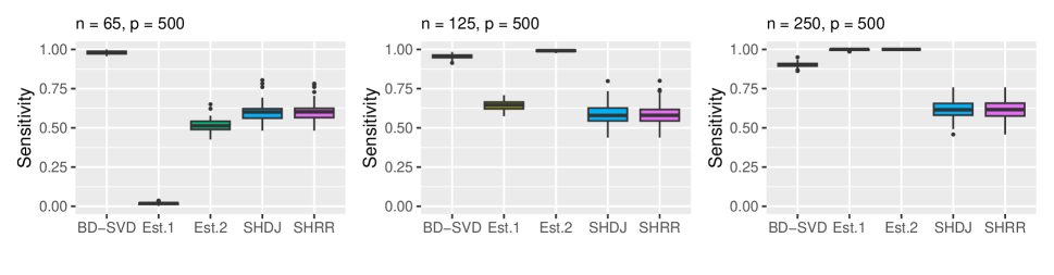
(a) Simulation design (a).

(b) Simulation design (b).

Figure 2: Simulation designs (a) and (b): Performance of BD-SVD, SHDJ, and SHRR for $(n,p)\in\{(65,500),\allowbreak(125,500),\allowbreak(250,500)\}$ measured by Sensitivity.

The results for both simulation designs are illustrated in Figure 2. Since there can be no false positive block detection for diagonal matrices, Specificity = 1 and FDR = 0 for these designs. Consequently, only the sensitivity is given.

3.2 Block Diagonal Covariance Structure

In this section, we examine scenarios in which the covariance matrix exhibits a block diagonal structure $\bm{\Sigma}=\operatorname{diag}(\bm{\Sigma}_{1},\ldots,\bm{\Sigma}_{b})$ with $b=10$ blocks $\bm{\Sigma}_{i}$ of equal sizes. Specifically, we consider two cases: (c) each block exhibits a compound symmetric covariance structure $\bm{\Sigma}_{i}=(1-\omega_{i})\bm{I}_{p_{i}}+2\omega_{i}\bm{1}_{p_{i}}\bm{1}_{p_{i}}^{\top}$ where $\omega_{i}$ is uniformly $U(0.1,0.3)$ distributed and $\bm{1}_{p_{i}}$ is a vector of ones, and (d) $\bm{\Sigma}_{i}=\bm{M}(i)$ where the components of $\bm{M}(l)=(m_{ij})$, simulated as $m_{ij}=(-1)^{i+j}\omega_{l}^{|i-j|^{0.05}}$ with $\omega_{l}\sim U(0.3,0.5)$, decrease in magnitude the further they move away from the diagonal. Across both simulation designs, we consider $(n,p)\in\{(250,500),\allowbreak(500,500),\allowbreak(500,2500),\allowbreak(500,5000)\}$ such that all blocks $\bm{\Sigma}_{i}$ are of equal size $p_{i}=p/b\in\{50,\allowbreak 250,\allowbreak 500\}$.

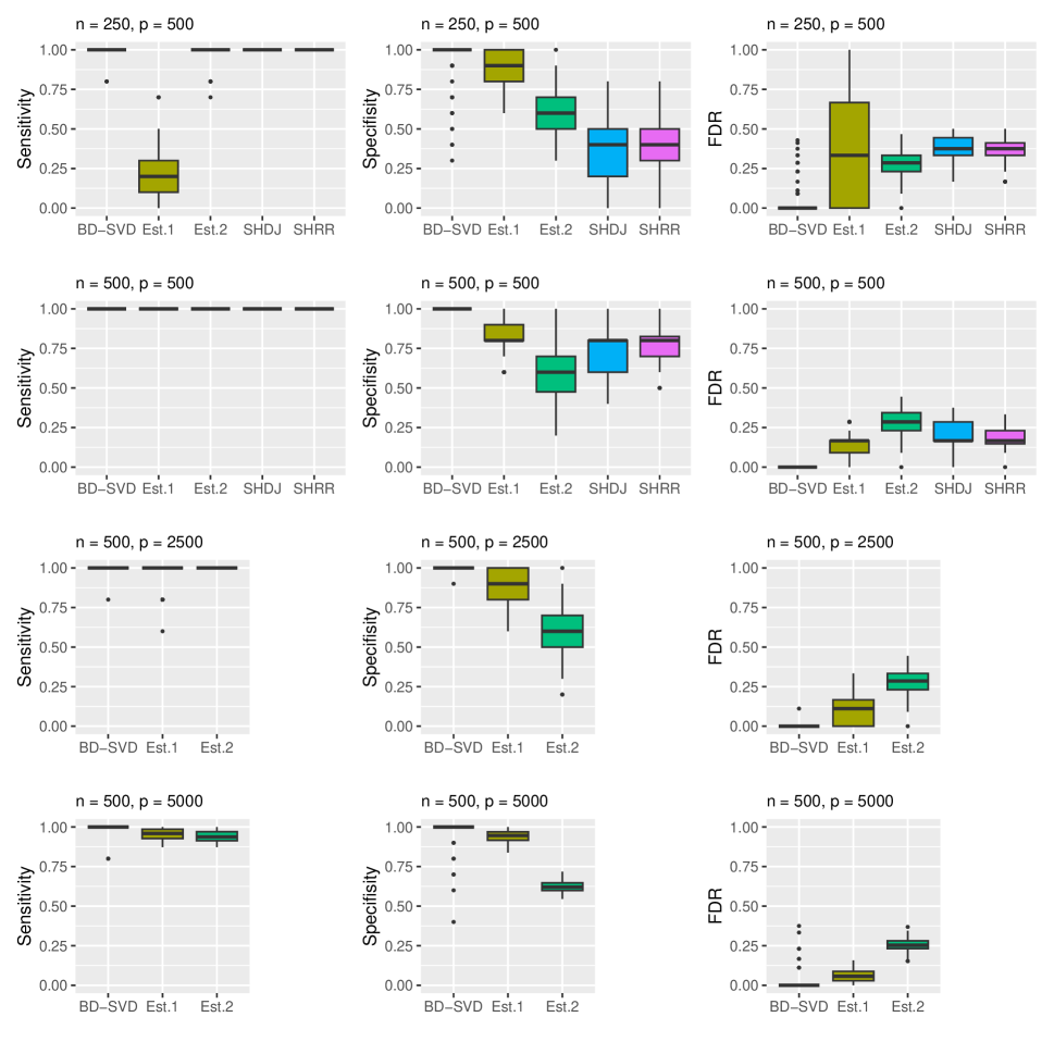
Figure 3: Simulation design (c): Performance of BD-SVD, Est_0.1, Est_0.2, SHDJ, and SHRR for $(n,p)\in\{(250,500),\allowbreak(500,500)\}$, and of BD-SVD, Est_0.1, and Est_0.2 for $(n,p)\in\{(500,2500),\allowbreak(500,5000)\}$ measured by Sensitivity, Specificity, and FDR.

The results for simulation designs (c) and (d) are illustrated in Figure 3 and Figure 4 respectively. Notably, the comparison of BD-SVD with SHDJ and SHRR was limited to cases where $p\leq 500$ due to the long running time of these methods in higher dimensions. In fact, the methods did not converge in our simulations when $p\geq 2500$.

BD-SVD outperforms the other methods across the simulation designs. It is worth noting that the ad hoc procedure shows decent performance, although not reliably across all designs. Intuitively, smaller values for $\tau$ lead to a higher sensitivity while large vales lead to a higher specificity.

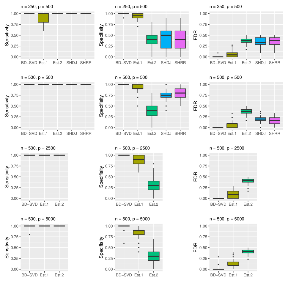
Figure 4: Simulation design (d): Performance of BD-SVD, Est_0.1, Est_0.2, SHDJ, and SHRR for $(n,p)\in\{(250,500),\allowbreak(500,500)\}$, and of BD-SVD, Est_0.1, and Est_0.2 for $(n,p)\in\{(500,2500),\allowbreak(500,5000)\}$ measured by Sensitivity, Specificity, and FDR.

3.3 A Note on Sparse Principal Component Analysis

Although both BD-SVD and SPCA employ sparse loadings to uncover data structures, they differ in their goals. While SPCA aims to identify sparse loadings explaining the most variance in the data matrix, BD-SVD targets sparse loadings fitting the population covariance matrix. Though their aims may occasionally align, they typically diverge.

To illustrate this, we ran SPCA on simulation design (c) and (d) with $n=500$, $p=500$, and $b=10$ such that $p_{i}=50$. Simplifying the process, we computed only the first SPCA loading. To determine the suitable sparseness for SPCA, we increased sparsity until the first sparse principal component explained at least 90% or 95% of the first principal component without sparseness constraints, a common practice in SPCA (Zou et al., 2006; Shen and Huang, 2008).

	Expl.	$n$	$p$	$b$	Sensitivity
Simulation design (c)	$0.90$	$500$	$500$	$10$	0.47
Simulation design (c)	$0.95$	$500$	$500$	$10$	0.67
Simulation design (d)	$0.90$	$500$	$500$	$10$	0.60
Simulation design (d)	$0.95$	$500$	$500$	$10$	0.70

Table 1: Sensitivity of the first sparse sparse principal component for simulation designs (c) and (d) Sparseness for SPCA was increased until the first sparse principal component explained at least $90\%$ or $95\%$ of the first principal component without sparseness constraints.

Table 1 contains the sensitivity analysis of the simulation study, indicating that SCPA is less effective than BD-SVD. It is important to emphasize that the study only evaluates whether the first sparse principal component reflects the block diagonal structure. To reveal the entire structure, SPCA must be continued iteratively for the detected blocks, which leads to a further decrease in sensitivity. Additionally, in this simulation study, we calculated the explained variance with respect to the known population eigenvalue. However, in high-dimensional contexts, estimating the eigenvalue poses challenges (see, e.g., Johnstone (2001), Baik and Silverstein (2006), and Paul (2007), among others), which impacts the performance of SPCA.

4 Real Data Examples

4.1 Lung Cancer Data

In this section, we illustrate BD-SVD using microarray gene expression signatures. Specifically, we analyze a lung cancer gene expression data set that consists of $203$ patient samples comprising 139 lung adenocarcinomas, 21 squamous cell carcinoma cases, 20 pulmonary carcinoid tumors, 6 small cell lung cancers, and 17 normal lung samples. The data and additional details can be found online in the supporting information section of the article by Bhattacharjee et al. (2001).

The original data set contains $12\,600$ gene expressions measured using the Affymetrix 95av2 GeneChip. Following procedures similar to Liu et al. (2008) and Rothman et al. (2009), we filter the genes using the ratio of the sample standard deviation and sample mean of each gene. We keep the $600$ genes with the highest ratio and the $600$ genes with the lowest ratio, and refer to them as high-ratio genes and low-ratio genes respectively. We then standardize the remaining genes so that each gene has a sample mean of 0 and a sample standard deviation of 1. After gene filtering, the data set contains $n=203$ patients with $p=1200$ genes.

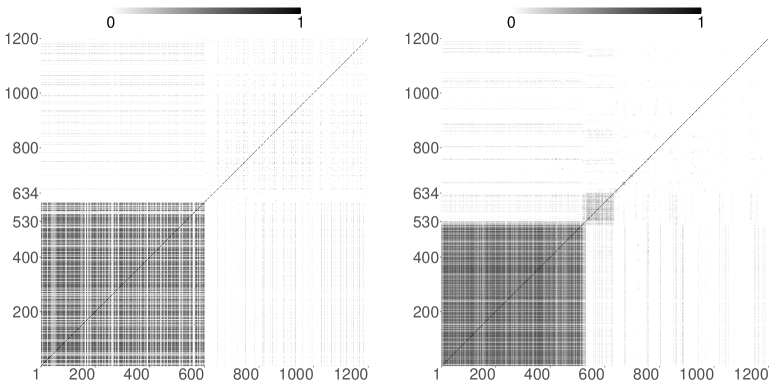
Figure 5: Sample covariance matrix with absolute values for the standardized gene expressions of the lung cancer data in its original data-ordering (left) and after reordering the variables based on the detected blocks $\bm{\Sigma}_{1},\ldots,\bm{\Sigma}_{217}$ (right).

The left plot in Figure 5 illustrates the sample covariance matrix of this subsample. We use absolute values of the estimated correlation coefficients because we are interested in the strength of the pairwise association between the genes, regardless of their sign. BD-SVD identifies 217 blocks $\bm{\Sigma}_{1},\ldots,\bm{\Sigma}_{217}$ with varying block sizes $p_{1}=530$, $p_{2}=104$, and $p_{i}\leq 3$ for $i\in\{3,\ldots,217\}$. Figure 5 (right) illustrates the sample covariance matrix after permuting variables according to the identified blocks.

A visual analysis of the first 600 variables in the left-hand plot, which correspond to the high-ratio genes, initially suggests a strong correlation structure, with little correlation between the low-ratio genes. However, BD-SVD detects a more refined structure. For example, the two largest blocks $\bm{\Sigma}_{1}$ and $\bm{\Sigma}_{2}$ contain a total of $p_{1}+p_{2}=634$ variables. Notably, $97.55\%$ of the variables in $\bm{\Sigma}_{1}$ and $81.55\%$ of the variables in $\bm{\Sigma}_{2}$ are high-ratio genes. On the other hand, $13.83\%$ of the variables contained in the remaining blocks $\bm{\Sigma}_{i}$ with $i\in\{3,\ldots,217\}$, i.e., all blocks except $\bm{\Sigma}_{1}$ and $\bm{\Sigma}_{2}$, are high-ratio genes. Thus, not all high-ratio genes are correlated with each other: Some high-ratio genes show no correlation with other high-ratio genes, while there are also cases in which low-ratio genes correlate with high-ratio genes.

4.2 Daily Stock Returns

In this section, we consider cross-sectional correlation of daily stock returns from various sectors from the S&P 500, including mining, quarrying, and oil and gas extraction sector; utilities sector; wholesale trade sector; retail trade sector; transportation and warehousing sector; information sector; finance and insurance sector; real estate and rental and leasing sector; professional, scientific, and technical services sector; administrative and support and waste management and remediation services sector; and arts, entertainment, and recreation sector. The data comes from the Center for Research in Security Prices and is available through Wharton Research Data Services. It consists of closing prices or bid/ask averages of 278 stocks on the trading days in the last quarter of 2022, which ranges from October 1, 2022 to December 31, 2022, encompassing a total of 63 days. Consequently, the data matrix consists of $n=63$ observations and $p=278$ variables.

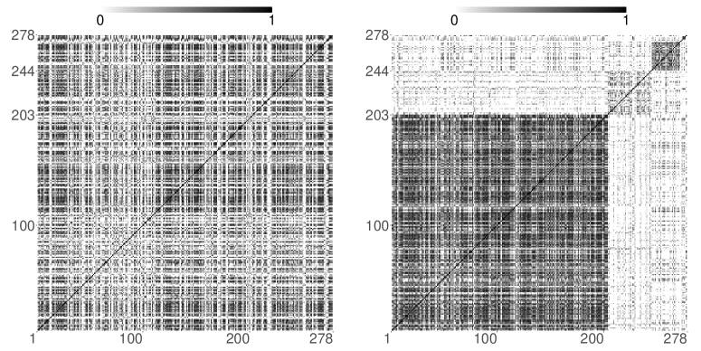
Figure 6: Sample covariance matrix with absolute values for the standardized daily stock returns data in its original data-ordering (left) and after reordering the variables based on the detected blocks $\bm{\Sigma}_{1},\ldots,\bm{\Sigma}_{5}$ (right).

We prepare the data matrix by standardizing it prior to our analysis. BD-SVD detects five blocks $\bm{\Sigma}_{1},\ldots,\bm{\Sigma}_{5}$ with $p_{1}=203$, $p_{2}=41$, $p_{3}=27$, $p_{4}=5$, and $p_{5}=2$. The sample covariance matrix, with variables permuted according to our findings, is illustrated in Figure 6. We use the absolute values of the estimated correlation coefficients for the reasons explained in the previous example.

5 Discussion

In this paper, we present a nonparametric method for detecting block diagonal structures in covariance matrices within high-dimensional data. Our approach relies on the first sparse loading ($k=1$) to mirror the underlying covariance matrix structure. Although we acknowledge the potential usefulness of employing $k>1$ sparse loadings, we intentionally limit our exploration of this scenario. This decision is motivated by the considerable accuracy achieved with the first loading only, coupled with potential drawbacks associated with using additional loadings. These drawbacks include increased computational costs and the risk of a stronger masking effect on the true structure of the covariance matrix. However, in our experience, these measures often resulted in incorrect covariance structures.

The choice of the appropriate degree of sparsity for the singular vectors plays a fundamental role in our methodology. To address this, we suggest to formulate the computation of the sparse loadings as a lasso regression problem. This allows us to use the HBIC to determine the appropriate sparsity level.

For completeness, we want to mention that in the course of our research we also experimented with other approaches to determine the appropriate degree of sparsity. For example, we tried cross validation to select the appropriate sparseness in our formulated lasso regression problem. However, as in the findings of Wang et al. (2007), this approach resulted in loadings that were not sufficiently sparse. To evaluate the validity of the detected blocks, we also considered dependency measures. In high-dimensional contexts, several methods have been developed to measure dependencies among subvectors (see, e.g., Székely and Rizzo (2013), Shen et al. (2020), Pan et al. (2020), Zhu et al. (2020), and Chatterjee (2021) among others). These measures typically yield zero values when the correlations between subvectors are zero. Furthermore, for our purposes, it would be necessary to establish a threshold value to determine when blocks can be considered uncorrelated.

BD-SVD has been implemented in the newly developed R package bdsvd [reference not given to maintaining blind review], which was written specifically for this research project.

SUPPLEMENTARY MATERIAL

The online supplementary materials contain derivations and proofs, and R code to perform the illustrative example and the simulation studies.

References

- Baglama et al. (2022) Baglama, J., L. Reichel, and B. W. Lewis (2022). irlba: Fast Truncated Singular Value Decomposition and Principal Components Analysis for Large Dense and Sparse Matrices. R package version 2.3.5.1.
- Bai et al. (2009) Bai, Z., D. Jiang, J.-F. Yao, and S. Zheng (2009). Corrections to LRT on large-dimensional covariance matrix by RMT. Ann. Stat. 37(6B), 3822–3840.
- Baik and Silverstein (2006) Baik, J. and J. W. Silverstein (2006). Eigenvalues of large sample covariance matrices of spiked population models. J. Multivar. Anal. 97(6), 1382–1408.
- Bao et al. (2017) Bao, Z., J. Hu, G. Pan, and W. Zhou (2017). Test of independence for high-dimensional random vectors based on freeness in block correlation matrices. Electron. J. Stat. 11(1), 1527–1548.
- Bauer and Drabant (2021) Bauer, J. O. and B. Drabant (2021). Principal loading analysis. J. Multivar. Anal. 184.
- Bhattacharjee et al. (2001) Bhattacharjee, A., W. G. Richards, J. E. Staunton, C. Li, S. Monti, P. P. Vasa, C. Ladd, J. Beheshti, R. Bueno, M. A. Gillette, M. Loda, G. Weber, E. J. Mark, E. S. Lander, W. Wong, B. E. Johnson, T. R. Golub, D. J. Sugarbaker, and M. L. Meyerson (2001). Classification of human lung carcinomas by mRNA expression profiling reveals distinct adenocarcinoma subclasses. Proc. Natl. Acad. Sci. U.S.A. 98, 13790–13795.
- Bickel and Levina (2008) Bickel, P. J. and E. Levina (2008). Covariance regularization by thresholding. Ann. Stat. 36(6), 2577–2604.
- Birke and Dette (2005) Birke, M. and H. Dette (2005). A note on testing the covariance matrix for large dimension. Statist. Probab. Lett. 74(3), 281–289.
- Boileau et al. (2021) Boileau, P., N. S. Hejazi, B. Collica, M. J. van der Laan, and S. Dudoit (2021). cvCovEst: Cross-validated covariance matrix estimator selection and evaluation in R. J. Open Source Softw. 6(63), 3273.
- Chatterjee (2021) Chatterjee, S. (2021). A new coefficient of correlation. J. Am. Stat. Assoc. 116(536), 2009–2022.
- Chen and Chen (2008) Chen, J. and Z. Chen (2008, 09). Extended Bayesian information criteria for model selection with large model spaces. Biometrika 95(3), 759–771.
- Chen et al. (2010) Chen, S. X., L.-X. Zhang, and P.-S. Zhong (2010). Tests for high-dimensional covariance matrices. J. Am. Stat. Assoc. 105(490), 810–819.
- Devijver and Gallopin (2015) Devijver, E. and M. Gallopin (2015). shock: Slope Heuristic for Block-Diagonal Covariance Selection in High Dimensional Gaussian Graphical Models. R package version 1.0.
- Devijver and Gallopin (2018) Devijver, E. and M. Gallopin (2018). Block-diagonal covariance selection for high-dimensional gaussian graphical models. J. Am. Stat. Assoc. 113(521), 306–314.
- Donoho and Johnstone (1994) Donoho, D. L. and I. M. Johnstone (1994). Ideal spatial adaptation by wavelet shrinkage. Biometrika 81(3), 425–455.
- Eckart and Young (1936) Eckart, C. and G. Young (1936). The approximation of one matrix by another of lower rank. Psychometrika 1, 211–218.
- Fan and Li (2001) Fan, J. and R. Li (2001). Variable selection via nonconcave penalized likelihood and its oracle properties. J. Am. Stat. Assoc. 96(456), 1348–1360.
- Fan and Li (2006) Fan, J. and R. Li (2006). Statistical challenges with high dimensionality: Feature selection in knowledge discovery. In Proceedings of the International Congress of Mathematicians, Volume 3, pp. 595–622. European Mathematical Society.
- Fan et al. (2013) Fan, J., Y. Liao, and M. Mincheva (2013). Large covariance estimation by thresholding principal orthogonal complements. J. R. Stat. Soc. B 75(4), 603–680.
- Fan and Tang (2012) Fan, Y. and C. Y. Tang (2012, 12). Tuning parameter selection in high dimensional penalized likelihood. J. R. Stat. Soc. B 75(3), 531–552.
- Fisher et al. (2010) Fisher, T. J., X. Sun, and C. M. Gallagher (2010). A new test for sphericity of the covariance matrix for high dimensional data. J. Multivar. Anal. 101(10), 2554–2570.
- Friedman et al. (2007) Friedman, J., T. Hastie, and R. Tibshirani (2007, 12). Sparse inverse covariance estimation with the graphical lasso. Biostatistics 9(3), 432–441.
- Gataric et al. (2020) Gataric, M., T. Wang, and R. J. Samworth (2020). Sparse principal component analysis via axis-aligned random projections. J. R. Stat. Soc. B 82(2), 329–359.
- Hyodo et al. (2015) Hyodo, M., N. Shutoh, T. Nishiyama, and T. Pavlenko (2015). Testing block-diagonal covariance structure for high-dimensional data. Stat. Neerl. 69(4), 460–482.
- James et al. (2021) James, G., D. Witten, T. Hastie, and R. Tibshirani (2021). An Introduction to Statistical Learning with Applications in R (2nd ed.). New York, USA: Springer.
- Jiang et al. (2013) Jiang, D., Z. Bai, and S. Zheng (2013). Testing the independence of sets of large-dimensional variables. Sci. China Math. 56, 135–147.
- Jiang and Yang (2013) Jiang, T. and F. Yang (2013). Central limit theorems for classical likelihood ratio tests for high-dimensional normal distributions. Ann. Stat. 41(4), 2029–2074.
- Johnstone (2001) Johnstone, I. M. (2001). On the distribution of the largest eigenvalue in principal components analysis. Ann. Stat. 29(2), 295–327.
- Johnstone (2008) Johnstone, I. M. (2008). Multivariate analysis and Jacobi ensembles: Largest eigenvalue, Tracy–Widom limits and rates of convergence. Ann. Stat. 36(6), 2638–2716.
- Johnstone and Lu (2009) Johnstone, I. M. and A. Y. Lu (2009). On consistency and sparsity for principal components analysis in high dimensions. J. Am. Stat. Assoc. 104(486), 682–693.
- Ledoit and Wolf (2002) Ledoit, O. and M. Wolf (2002). Some hypothesis tests for the covariance matrix when the dimension is large compared to the sample size. Ann. Stat. 30(4), 1081–1102.
- Leung and Drton (2018) Leung, D. and M. Drton (2018). Testing independence in high dimensions with sums of rank correlations. Ann. Stat. 46(1), 280–307.
- Liu et al. (2008) Liu, Y., D. N. Hayes, A. Nobel, and J. S. Marron (2008). Statistical significance of clustering for high-dimension, low–sample size data. J. Am. Stat. Assoc. 103(483), 1281–1293.
- Pan et al. (2020) Pan, W., X. Wang, H. Zhang, H. Zhu, and J. Zhu (2020). Ball covariance: A generic measure of dependence in banach space. J. Am. Stat. Assoc. 115(529), 307–317.
- Paul (2007) Paul, D. (2007). Asymptotics of sample eigenstructure for a large dimensional spiked covariance model. Stat. Sin. 17(4), 1617–1642.
- Pavlenko et al. (2012) Pavlenko, T., A. Björkström, and A. Tillander (2012). Covariance structure approximation via glasso in high-dimensional supervised classification. J. Appl. Stat. 39(8), 1643–1666.
- R Core Team (2022) R Core Team (2022). R: A Language and Environment for Statistical Computing. Vienna, Austria: R Foundation for Statistical Computing.
- Rothman et al. (2009) Rothman, A. J., E. Levina, and J. Zhu (2009). Generalized thresholding of large covariance matrices. J. Am. Stat. Assoc. 104(485), 177–186.
- Schott (2005) Schott, J. R. (2005). Testing for complete independence in high dimensions. Biometrika 92(4), 951–956.
- Schwarz (1978) Schwarz, G. (1978). Estimating the dimension of a model. Ann. Stat. 6(2), 461–464.
- Shen et al. (2020) Shen, C., C. E. Priebe, and J. T. Vogelstein (2020). From distance correlation to multiscale graph correlation. J. Am. Stat. Assoc. 115(529), 280–291.
- Shen et al. (2013) Shen, D., H. Shen, and J. S. Marron (2013). Consistency of sparse PCA in high dimension, low sample size contexts. J. Multivar. Anal. 115, 317–333.
- Shen and Huang (2008) Shen, H. and J. Z. Huang (2008). Sparse principal component analysis via regularized low rank matrix approximation. J. Multivar. Anal. 99(6), 1015–1034.
- Srivastava and Reid (2012) Srivastava, M. S. and N. Reid (2012). Testing the structure of the covariance matrix with fewer observations than the dimension. J. Multivar. Anal. 112, 156–171.
- Székely and Rizzo (2013) Székely, G. J. and M. L. Rizzo (2013). The distance correlation t-test of independence in high dimension. J. Multivar. Anal. 117, 193–213.
- Székely et al. (2007) Székely, G. J., M. L. Rizzo, and N. K. Bakirov (2007). Measuring and testing dependence by correlation of distances. Ann. Stat. 35(6), 2769–2794.
- Tan et al. (2015) Tan, K. M., D. Witten, and A. Shojaie (2015). The cluster graphical lasso for improved estimation of gaussian graphical models. Comput. Stat. Data Anal. 85, 23–36.
- Tibshirani (1996) Tibshirani, R. (1996). Regression shrinkage and selection via the lasso. J. R. Stat. Soc. B 58(1), 267–288.
- Wang et al. (2009) Wang, H., B. Li, and C. Leng (2009). Shrinkage tuning parameter selection with a diverging number of parameters. J. R. Stat. Soc. B 71(3), 671–683.
- Wang et al. (2007) Wang, H., R. Li, and C.-L. Tsai (2007, 08). Tuning parameter selectors for the smoothly clipped absolute deviation method. Biometrika 94(3), 553–568.
- Wang et al. (2013) Wang, L., Y. Kim, and R. Li (2013). Calibrating nonconvex penalized regression in ultra-high dimension. Ann. Stat. 41(5), 2505–2536.
- Witten et al. (2009) Witten, D. M., R. Tibshirani, and T. A. Hastie (2009). A penalized matrix decomposition, with applications to sparse principal components and canonical correlation analysis. Biostatistics 10(3), 515–534.
- Yamada et al. (2017) Yamada, Y., M. Hyodo, and T. Nishiyama (2017). Testing block-diagonal covariance structure for high-dimensional data under non-normality. J. Multivar. Anal. 155, 305–316.
- Yang et al. (2014) Yang, D., Z. Ma, and A. Buja (2014). A sparse singular value decomposition method for high-dimensional data. J. Comput. Graph. Stat. 23(4), 923–942.
- Yata and Aoshima (2016) Yata, K. and M. Aoshima (2016). High-dimensional inference on covariance structures via the extended cross-data-matrix methodology. J. Multivar. Anal. 151, 151–166.
- Yu et al. (2015) Yu, Y., T. Wang, and R. J. Samworth (2015). A useful variant of the Davis—Kahan theorem for statisticians. Biometrika 102(2), 315–323.
- Zhu et al. (2020) Zhu, C., X. Zhang, S. Yao, and X. Shao (2020). Distance-based and RKHS-based dependence metrics in high dimension. Ann. Stat. 48(6), 3366–3394.
- Zou et al. (2006) Zou, H., T. Hastie, and R. Tibshirani (2006). Sparse principal component analysis. J. Comput. Graph. Stat. 15(2), 265–286.
- Zou et al. (2007) Zou, H., T. Hastie, and R. Tibshirani (2007). On the “degrees of freedom” of the lasso. Ann. Stat. 35(5), 2173–2192.