The Quantum Mechanical Problem of a Particle on a Ring with Delta Well

Abstract.

The problem of a spin-free electron with mass $m$, charge $e$ confined onto a ring of radius $R_{0}$ and with an attractive Dirac delta potentential with scaling factor (depth) $\kappa$ in non-relativistic theory has closed form analytical solutions. The single bound state function is of the form of a hyperbolic cosine that however contains a paramter $d>0$ which is the single positive real solution of the transcentdental equation $\coth(d)=\lambda d$ for non zero real $\lambda=\frac{2}{\pi\kappa}$. The energy eigenvalue of the bound state $\varepsilon=-\frac{d^{2}}{2\pi^{2}}\approx\frac{qemR_{0}}{2\hbar^{2}}$. In addition a discrete inifinty of unbounded solutions exists, formally they are obtained from the terms for the bound solution by substituting $d\to id$ yielding $\cot(d)=\lambda d$ as characteristic equation with the correspondig set of solutions $d_{k},k\in\mathbb{N}$, the respective state functions obtain via $\cosh(x)\overset{x\to ix}{\longrightarrow}\cos(x)$ of the form of cosine functions.

1. Introduction

There is only roughly a dozen of quantum mechanical (QM) systems with an analytical solution.[Wikipedia contributors(2022)] QM problems with analytical solutions are not only of great of didactical use for showin how these problems can be solved but often serve also as physical toy model systems for otherwise unsovable problems which however share the principal characteristics.

One example herefore is the particle in the Dirac delta potential[Wikipedia contributors(2022)] which not ony serves with its bound state as an one-dimensional analog of the hydrogen atom but can also be interpreted as the simplest model for electron scattering when one regards the unbound states and allows for simple calculation of reflection and transmissoin rates on step- and related potentials, which is for example of relevance for the theory of scanning tunnel microscopy.

In the context of our research on symmetry breaking in rotationally invariant systems[Berger and Viel(2020)] we came across the analogous problem where the particle is but confined to an atomic scale ring. As it turned out that this QM model system has not yet been described in the literature (to the best of our knowledge) we report on our results in the following.

2. Solution

2.1. Schrödinger equation

A spin-free electron (i.e. a particle with charge $-e$ and mass $m_{e}$) on in a ring shaped space with radius $R_{0}$ and a $\delta$ function well of amplitude $-qe$ corresponding to an attractive potential with an integrated total charge of $+qe$ is regarded in non-relativistic quantum mechanic theory.

As is well known from textbooks the Hamiltonian for the particle on a ring of radius $R_{0}$ in 2D polar coordinates ($r\in\mathbb{R}^{+},\vartheta\in[0,2\pi)$) in SI units is given by

(1) $$\hat{H^{\prime}} =-\frac{\hbar^{2}}{2mR_{0}^{2}}\frac{\partial^{2}}{\partial\vartheta^{2}}$$

The ring shall contain an attractive potential $\hat{V}$ with respect to the electron in the form of a Dirac-$\delta$ function and the potential shall integrate over the whole space ($R_{0}\times[0,2\pi)$) to the product of electron and potential charge of $-eq<0$:

(2) $$\hat{V} =-qe\delta((\vartheta-\vartheta_{0})l),$$

were $\vartheta$ is given in units of $\mathrm{[}rad]$, thus formally $l=1\mathrm{rad}^{-1}=1\frac{1m}{1m}=1$ and hence can be dropped in the following. Without loss of generality we will set $\vartheta_{0}=0$ such that the Schrödinger equation for the problem becomes

$$\hat{H}\psi(\vartheta) =E\psi(\vartheta)$$

$$(\hat{H^{\prime}}+\hat{V})\psi(\vartheta) =E\psi(\vartheta)$$

(3) $$\left(-\frac{\hbar^{2}}{2mR_{0}^{2}}\frac{\partial^{2}}{\partial\vartheta^{2}}-qe\delta(\vartheta)\right)\psi(\vartheta) =E\psi(\vartheta)$$

$$\left(\frac{\partial^{2}}{\partial\vartheta^{2}}+\frac{2qemR_{0}^{2}}{\hbar^{2}}\delta(\vartheta)+E\frac{2mR_{0}^{2}}{\hbar^{2}}\right)\psi(\vartheta) =0$$

For simplicity we combine the constants in

(4) $$\kappa=\frac{2qemR_{0}^{2}}{\hbar^{2}}$$

and

(5) $$\epsilon=\frac{2mR_{0}^{2}}{\hbar^{2}}E$$

such that we obtain

(6) $$\psi^{\prime\prime}+(\epsilon+\kappa\delta)\psi =0$$

2.2. Bound state ($E<0$)

The assumption of $(E-V)<0$ or (ignoring the singularity at the origin) $E<0$, or $\epsilon<0$, respectively thus leads to the bound state solutions. For the symmetry of the problem and the form of the differential equation (6) we chose the Ansatz

(7) $$\psi(\vartheta;d)=N^{\prime}(e^{-d\vartheta}+e^{d(\vartheta-2\pi)})=N\cosh(d(x-\pi))$$

Yielding the normalization constant

(8) $$N=\sqrt{\frac{\sinh(2\pi d)}{2d}+\pi}^{-1}$$

To determine the exponent $d$ one in principle has to insert (7) into (6) and attempt to match $d$ to the boundary conditions. One boundary condition, the symmtry of the system, was already accounted for choosing the same exponent $d$ for both functions but with different sign. Since a $\delta$-function is appearing one has to chose an appropriate strategy to evaluate the result of combining (7) and (6). The strategy is to integrate the Schrödinger equation in an $\epsilon$ ball around the origin of the $\delta$-function and to perform the limit of $\epsilon\to 0$, this results in

$$\lim_{\epsilon\to 0}\int_{0-\epsilon}^{0+\epsilon}\left(\frac{\partial^{2}}{\partial\vartheta^{2}}\psi(\vartheta)\right)+\kappa\delta(\vartheta)\psi(\vartheta)-E^{\prime}\psi(\vartheta)\;d\vartheta =\lim_{\epsilon\to 0}\int_{0-\epsilon}^{0+\epsilon}0d\vartheta$$

(9) $$\psi^{\prime}(0^{+})-\psi^{\prime}(0^{-})+\kappa\psi(0) =0$$

Inserting (7) in (9) yields

$$-2d+2de^{-2\pi d}+\kappa(1+e^{-2\pi d}) =0$$

(10) $$\coth(\pi d) =\frac{2}{\kappa}d$$

using $d^{\prime}=\pi d$ and $\lambda=\frac{2}{\pi\kappa}$ we obtain

(11) $$\coth(d^{\prime}) =\lambda d^{\prime}$$

here for $\lambda>0$ and real $d^{\prime}$ exactly one pair of solutions $d^{\prime}_{+}=-d^{\prime}_{-}$ exists and yielding the same function $\psi(\vartheta;d)$ due to the axial symmetry of $\cosh$, hence we can drop the $\pm$ indices in the following and only regard the positive solution $d^{\prime}$, which is it the same time the only solution to (6).

Equation (11) has no symbolic closed form solution, but

(12) $$\coth(d^{\prime})\approx 1$$

holds with accuracy increasing in $d^{\prime}$ (see Fig. 1).

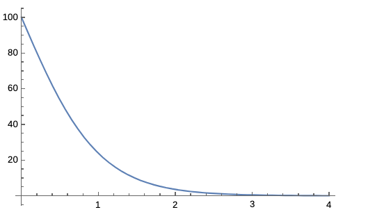
Figure 1. Realtive error in % obtained from using (12) in dependence on $d^{\prime}$

Using (12) the solution of (10) can be approximated as

$$d\approx d^{0}=\frac{\kappa}{2}=\frac{qemR_{0}^{2}}{\hbar^{2}}$$

with deviations decreasing with charge and ring size. In the Table 1 some exemplary values for $R_{0}$ set to 1 (all atomic units) are shown. At $R_{0}=1$ bohr and $q=1e$ we have $\epsilon=-d^{2}=-\frac{d^{\prime 2}}{\pi^{2}}$ and $E=-\frac{d^{\prime 2}\hbar^{2}}{2m\pi^{2}R_{0}^{2}}\approx-0.0145$ Hartree (for comparision in the approximation (12) it yields $E^{0}=-\frac{{d^{0}}^{2}}{\pi^{2}}\approx-0.0127$ Hartree (further values are listed in Table 1). In addition we note that with increasing radius $R_{0}$ the approximative solutions will be of increasing quality.

$q$	1	2	3	4	5
${d^{0}}^{\prime}$	0.5	1.0	1.5	2.0	2.5
$d^{\prime}$	0.53575	1.00366	1.50024	2.00001	2.5
${E^{0}}^{\prime}$	-0.01267	-0.05066	-0.11399	-0.202642	-0.31663
$E^{0}$	-0.01454	-0.05103	-0.11402	-0.202642	-0.31663

Table 1. Numerically exact ($d^{\prime}$) and approximated solutions (${d^{0}}^{\prime}$) of (10) at different total charges $q$ of the Dirac delta potential and corresponding approximate (${E^{0}}^{\prime}$) and numerically exact energies (${E^{0}}^{\prime}$) at $1$ Bohr radius.

A graphical display of the wave function of the bound state is shown in Fig. 2.

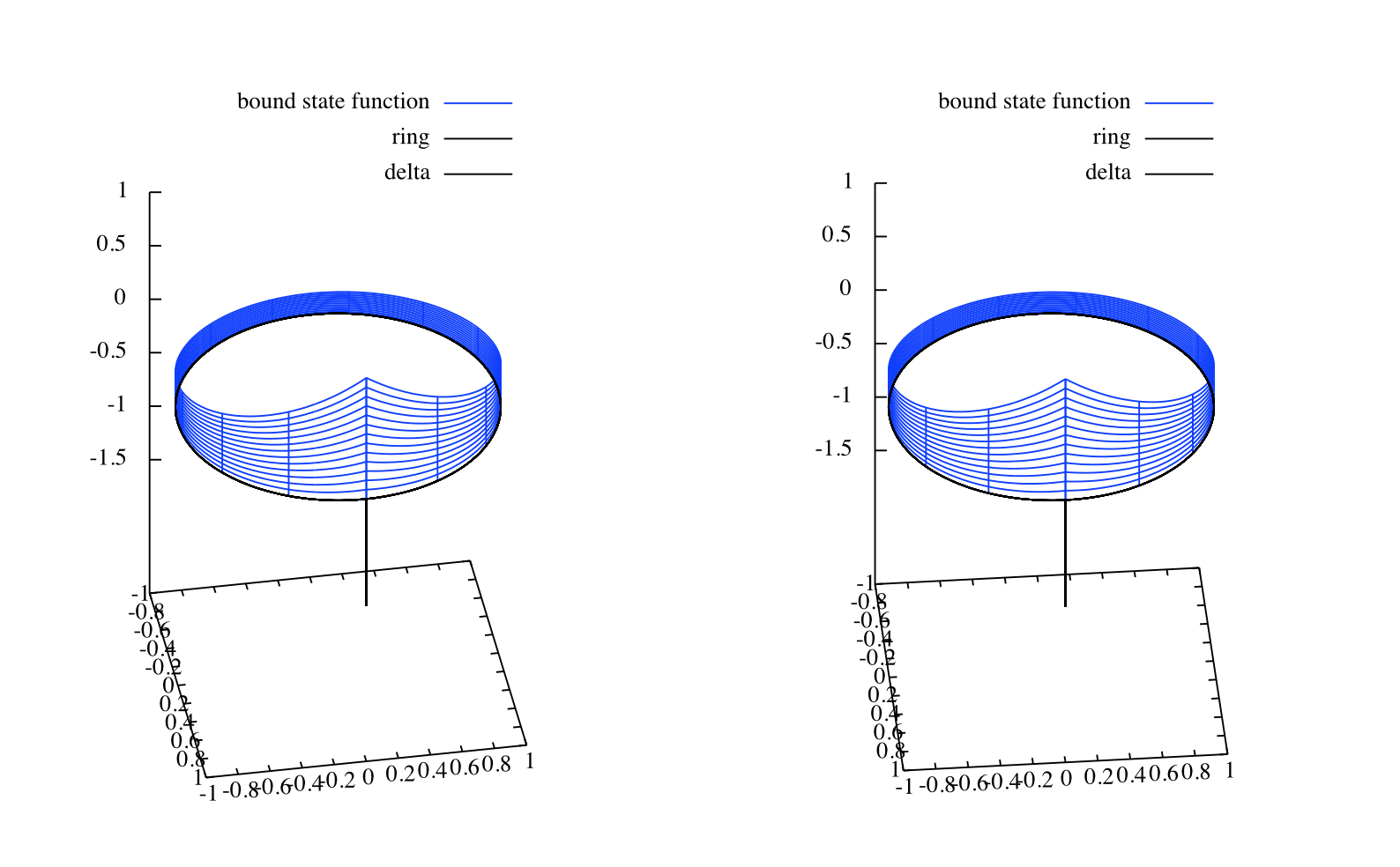
Figure 2. Stereographic projection of $\psi(\vartheta)$ for the bound state of the partice in the ring with $\delta$ well.

2.3. Unbound states ($E>0$)

In the spirit of (7) the unbound states can be obtained from the Ansatz

(13) $$\psi(\vartheta;di)=C(e^{-di\vartheta}+e^{di(\vartheta-2\pi)})$$

Yielding in analogy to (10)

$$-2id+2ide^{-i2\pi d}+\kappa(1+e^{-i2\pi d}) =0$$

(14) $$\cot(\pi d) =\frac{2}{\kappa}d$$

In contrast to (10) this yields for finite positive $\kappa$ an infinite set of solutions. As in (10) the system is strictly not analytically solvable in terms of a finite closed expression. However, for sufficiently large $d$ or large values of $\kappa$ the solutions are approaching

(15) $$d_{n_{+/-}}\approx d^{(0)}_{n_{+/-}}=\pm n\frac{\kappa}{2}$$

The first 5 unbound solutions for $d$ and the corresponding energies of the sytem with charge $+1e$ and $R=1$ bohr are

$n$	1	2	3	4	5
$d^{(0)}_{n_{+}}$	0.5	1.0	2.0	3.0	4.0
$d_{n_{+}}$	0.34278	1.15979	2.09395	3.06518	4.04963
$E_{n}$	0.05875	0.67256	2.19231	4.69766	8.19976

Since $\psi(\vartheta;di)$ are not purely real functions, we first decompose them into real and imaginary part

(16) $$\Re{[\psi(\vartheta;di)]} =C[\cos(d\vartheta)+\cos(d(2\pi-\vartheta))]$$

(17) $$=\left(\frac{\sin(2\pi d)}{2d}+\pi\right)^{-\frac{1}{2}}\cos[d(\pi-\vartheta^{\prime})]$$

(18) $$\Im{[\psi(\vartheta;di)]} =C[\sin(d\vartheta)+\sin(d(2\pi-\vartheta))]$$

and we note that (18) in general is dicontinuous at the $\delta$ well, thus must be rejected. (16) can be rewritten as a single cosine function originating at the position opposing the origin $\vartheta^{\prime}_{o}=\pi$

$$\Re{[\psi(\vartheta;di)]} =2C\cos(d\pi)[\cos(d(\pi-\vartheta))]$$

(19) $$=C^{\prime}\cos[d(\pi-\vartheta^{\prime})]$$

with $-\pi\leq\vartheta^{\prime}<\pi$ and the normalisation constant

(20) $$C^{\prime}=\left(\frac{\sin(2\pi d)}{2d}+\pi\right)^{-\frac{1}{2}}$$

In summary this yields the unbounded state functions

(21) $$\psi_{n} =\sqrt{\frac{\sin(4\pi d_{n})}{4d_{n}}+\pi}^{-1}\cos[d_{n}(\pi-\vartheta)]$$

for $-\pi\leq\vartheta<\pi$ and $n>0$ with energies

(22) $$E_{n}=-\frac{\hbar^{2}}{2mR_{0}^{2}}d_{n}^{2}$$

where $d_{n}$ are corresponding to the positive solutions of

(23) $$\cot(\pi d_{n}) =\frac{2\pi\hbar^{2}}{qemR_{0}}d_{n}.$$

which are approximated for large $q$, $R_{0}$ or $n$ by

(24) $$d_{n}\approx d^{0}_{n}=n\frac{qR_{0}em}{2\pi\hbar^{2}}$$

where we have removed the symmetry equivalent negative solutions, since $\cos$ is an even function, thus droped the sign indices, as compared to (15). Hereby we note that in comparison to the particle in the ring (without additional well potential) we have lost the two-fold degeneracy of the higher (non-ground) states. Which is an obvious consequence of the symmetry breaking due to the potential.

2.4. $\kappa$ dependence

The $\kappa$ dependence of the real solutions of (28) is illustrated in the graph below. The approximative solutions (24) we have used are based on the asymptotic approximation of the $\tan$ branches to $x=2n+1$ for $n\in\mathbb{R}$.

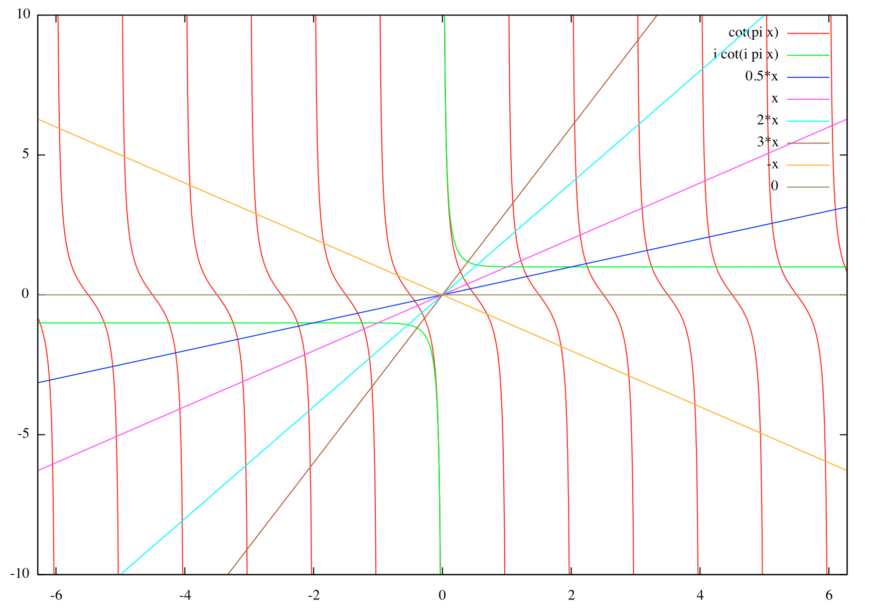
Figure 3. Graphical representation of the solutions of the characteristic equation (23) for the problem with $\kappa=2$

3. Smooth wave function for the bound state

Independently of the physical significance, one can ask for conditions under which the wave function becomes smooth at the position of the Dirac delta function potential. Smoothness at $\vartheta=0$ requires $d=1/2$ in the bounded state (7). Hence we obtain from (10), (4) and using atomic units

(25) $$R_{0}=\sqrt{\frac{\tanh{\pi/2}}{2q}}$$

yielding, e.g. $R_{0}=0.677183$ Bohr for $q=1$ at $E_{0}=-0.01267$ Hartree.

4. Summary

Due to the relations $\cos(ix)=\cosh(x)$ and $\sin(ix)=\sinh(x)$ we can combine the bound (7) and the unbound (21) solutions in one expression

(26) $$\psi_{n} =\sqrt{\frac{\sin(4\pi a_{n})}{4a_{n}}+\pi}^{-1}\cos[a_{n}(\pi-\vartheta)]$$

with $\kappa=qR_{0}\frac{em}{\pi\hbar^{2}}$, and the corresponding energies

(27) $$E_{n}=\frac{\hbar^{2}}{2mR_{0}^{2}}a_{n}^{2},\;\;\forall n\in\mathbb{N}_{0}.$$

and where $a_{0}$ is the (single) purely imaginary solution and $a_{n}$ with $n>0$ are the purely real solutions of the equation

(28) $$\cot(\pi a)=\frac{2}{\kappa}a$$