Bayesian Multivariate Quantile Regression with alternative Time-varying Volatility Specifications

Abstract

This article proposes a novel Bayesian multivariate quantile regression to forecast the tail behavior of US macro and financial indicators, where the homoskedasticity assumption is relaxed to allow for time-varying volatility. In particular, we exploit the mixture representation of the multivariate asymmetric Laplace likelihood and the Cholesky-type decomposition of the scale matrix to introduce stochastic volatility and GARCH processes, and we provide an efficient MCMC to estimate them. The proposed models outperform the homoskedastic benchmark mainly when predicting the distribution’s tails. We provide a model combination using a quantile score-based weighting scheme, which leads to improved performances, notably when no single model uniformly outperforms the other across quantiles, time, or variables.

Keywords: Bayesian inference; forecasting; model combination; multivariate quantile regression; time-varying volatility.

1 Introduction

The current global economic and financial situation caused by the COVID-19 pandemic and the Russian-Ukrainian war has renewed the interest of the economic forecasters’ and policy institutions in tail risk. In particular, there has been an increased interest in understanding, modeling, and forecasting the macroeconomic downside tail risk and in quantifying the uncertainty around these predictions. Typical time series methods model the conditional mean of variables of interest, making them unsuited to capture features, such as skewness, fat tails, and outliers, that typically characterize economic and financial time series in turbulent periods. To answer these questions, quantile regression models (QR, see Koenker and Bassett, 1978) have been exploited to study the heterogeneous impact of covariates on different quantile levels of a variable of interest. In particular, we contribute to this growing literature by extending recently introduced multivariate QR framework to account for alternative time-varying volatility specifications, with the aim of enhancing the forecasting performance of economic and financial indicators.

Within the macroeconomic literature, Adrian et al. (2019) use QR to estimate the predictive distribution of real GDP growth as a function of financial and economic conditions. In a follow-up, Adrian et al. (2022) define the growth-at-risk (GaR) as the effect on the lower $5$th percentile of conditional growth and estimate it by applying a panel quantile regression model to a collection of eleven advanced economies. This approach has been recently extended in Ferrara et al. (2022), who introduce mixed-data sampling (MIDAS) to a Bayesian QR model to leverage on the informational content of high-frequency financial conditions indicators. Adams et al. (2021) use a QR model to characterize upside and downside risks around the Survey of Professional Forecasters and provide a forward-looking assessment of uncertainty, which captures asymmetries in risks and allows for the construction of informative tail risk measures. In macroeconomic forecasting, univariate quantile autoregressive models have been used for making more accurate predictions on the tails of the predictive distribution of key variables, such as the GDP. Recently, Carriero et al. (2022) proposed to nowcast tail risk to GDP growth by using Bayesian quantile regression and mixed-frequency regression with stochastic volatility, whereas Pfarrhofer (2022) introduced time-varying parameters in quantile regression to dynamically trace the quantiles of inflation.

More recent contributions have extended quantile regression to the multivariate setting, originating the quantile Vector autoregressive (QVAR) models, among the others. Chavleishvili and Manganelli (2021) introduce a structural QVAR model to capture nonlinear relationships among macroeconomic variables and define a quantile impulse response function to perform stress tests. Aastveit et al. (2022) develop a forecasting combination scheme from Bayesian quantile regressions that assigns weights to the individual predictive density forecasts based on the quantile scores. Iacopini et al. (2022) introduce a novel mixed-frequency quantile VAR model (MF-QVAR), which combines different frequencies in macroeconomic and financial variables to nowcast conditional quantiles of the US GDP.

Quantile regression models rely on the asymmetric Laplace distribution (Kotz et al., 2001) for defining the likelihood. Its representation as a location-scale mixture of Gaussian distributions has allowed the design of efficient estimation algorithms (e.g., see Kozumi and Kobayashi, 2011). But it also complicates the introduction of temporal variation for the scale parameter. We fill-in this gap and propose two frameworks for time-varying volatility in multivariate quantile regression models by means of a parameter-driven and an observation-driven specification. Specifically, we define the likelihood of a QVAR model via the multivariate asymmetric Laplace (MAL) distribution as in Iacopini et al. (2022) and Petrella and Raponi (2019), then we model the conditional variance with either stochastic volatility (SV, Cogley and Sargent, 2005; Primiceri, 2005) or generalized autoregressive conditional heteroskedasticity (GARCH, Engle, 1982; Bollerslev, 1986).

Both extensions have nontrivial computational implications, as coupling SV or GARCH effects with the mixture of Gaussian representation of the asymmetric Laplace distribution results in the volatility affecting also the conditional mean of the conditionally Gaussian distribution, but differently from the traditional SV- or GARCH-in-mean models. As a consequence, traditional methods for sampling the volatility path in SV- or GARCH-in-mean models may be highly inefficient in this quantile framework. As a further contribution, we address this issue by reformulating the models to make possible the joint sampling of the whole trajectory of the time-varying volatility, independently along the cross-sectional dimension.

As widely shown in the macroeconomic literature (D’Agostino et al., 2013; Clark and Ravazzolo, 2015; Carriero et al., 2016), introducing alternative time-varying volatility specifications improves the forecasting performance of conditional mean models, particularly in multivariate frameworks. However, most of the existing QR models impose constant volatility for the observables, which is a rather restrictive assumption when investigating economic and financial time series data, see Caporin et al. (2018) and Caporin et al. (2021) for exceptions. Moreover, whereas a number of studies in the macroeconomic literature have compared quantile univariate models, no comparisons between different time-varying volatility models have been proposed.

We propose to address these issues by first introducing the QVAR-SV and QVAR-GARCH models. Then, motivated by the lack of a systematic comparison of the performance of quantile regression methods for multivariate time series, this article compares several univariate and multivariate quantile regression models with constant and alternative time-varying volatility specifications, adopting a Bayesian approach to inference as in Clark and Ravazzolo (2015). The forecasting exercise considers different quantiles for several key macroeconomic indicators and compares a plethora of models differing for the dimensionality (univariate and multivariate) and the assumed volatility process (constant and time-varying) settings. Finally, model combinations are considered based on quantile score weighting schemes (Aastveit et al., 2022).

The QVAR-SV and QVAR-GARCH models are compared in forecasting US economic and financial data, namely the GDP, unemployment rate, inflation, and the NFCI. The results show that the proposed methods beat the constant volatility QVAR benchmark for all the variables investigated, however no single specification is found to uniformly dominate the other ones over time, nor across variables or quantiles. Therefore, to provide the forecaster with a practical method that accommodates the wide changes of the forecasting performance of individual models, we propose a model combination with a quantile score-based weighting scheme. The combination weights show significant variation over time, especially when the quantiles corresponding to the tails of the distribution are concerned, and at each point in time most of the mass is assigned to a single model.

The remainder of this article is organized as follows: Section 2 presents two novel quantile regression models with time-varying volatility. Section 3 illustrates the Bayesian approach to inference and the combination weights scheme. Then, Section 4 provides forecasting evidence based on the quantile score for the US quarterly macroeconomic data. Finally, Section 5 concludes the article.

2 Quantile regression models with alternative time-varying volatility specification

Let $\mathbf{y}_{t}\in\mathds{R}^{n}$ be an $n$-dimensional vector of response and $\mathbf{x}_{t}\in\mathds{R}^{k}$ be a $k$-dimensional vector of common covariates. Following the parametrization in Petrella and Raponi (2019), we define a multivariate quantile regression model as:

$$\mathbf{y}_{t}=B\mathbf{x}_{t}+\bm{\epsilon}_{t},\qquad\bm{\epsilon}_{t}\sim\text{MAL}_{n}(\mathbf{0},D\bm{\theta}_{1},D\Theta_{2}\Psi\Theta_{2}D),$$ (1)

where $B$ is a $(n\times k)$ coefficient matrix, and $\text{MAL}_{n}(\bm{\mu},\bm{\xi},\Sigma)$ denotes the multivariate asymmetric Laplace distribution (Kotz et al., 2001), with location $\bm{\mu}\in\mathds{R}^{n}$, skew parameter $\bm{\xi}\in\mathds{R}^{n}$, and positive definite scale matrix $\Sigma$. The parametrization of eq. (1) is such that $D=\operatorname{diag}(\delta_{1},\ldots,\delta_{n})$ with $\delta_{j}>0$, $\Psi$ is a correlation matrix, and $\Theta_{2}=\operatorname{diag}(\bm{\theta}_{2})$, with:

$$\theta_{1,j}=\frac{1-2\tau_{j}}{\tau_{j}(1-\tau_{j})},\qquad\theta_{2,j}=\frac{2}{\tau_{j}(1-\tau_{j})},\qquad j=1,\ldots,n,$$ (2)

where $\tau_{j}\in(0,1)$ is the (marginal) quantile of the $j$th series. Building on the mixture representation of the multivariate asymmetric Laplace distribution, one obtains:

$$\mathbf{y}_{t} =X_{t}\bm{\beta}+D\bm{\theta}_{1}w_{t}+\sqrt{w_{t}}D\Theta_{2}\Psi^{1/2}\mathbf{z}_{t},\qquad\mathbf{z}_{t}\sim\mathcal{N}_{n}(\mathbf{0},I_{n}),\quad w_{t}\sim\mathcal{E}xp(1),$$ (3)

where $\bm{\beta}=\operatorname{vec}(B)\in\mathds{R}^{nk}$ is the vectorized coefficient matrix, $\bm{\theta}_{1}=(\theta_{1,1},\ldots,\theta_{1,n})$, and $X_{t}=(I_{n}\otimes\mathbf{x}_{t})$.

The multivariate QR in eq. (3) includes the quantile VAR (QVAR) model as a special case for $\mathbf{x}_{t}=\mathbf{y}_{t-1}$. However, it assumes homoskedastic variance for the conditional distribution of the response variables, $\mathbf{y}_{t}$, which is highly restrictive when modeling economic and financial time series as they are typically characterized by highly persistent and clustered volatility. The most popular solutions when modeling the conditional mean are the stochastic volatility (Taylor, 1986) and the GARCH (Bollerslev, 1986) specifications, which belong to the general classes of parameter-driven and observation-driven models (Cox et al., 1981), respectively. Wit the aim of introducing similar dynamics for the time-varying volatility in the conditional distribution of $\mathbf{y}_{t}$ in eq. (3), we first reparametrize the model as follows.

Let us denote by $\Sigma=D\Psi D$ a positive definite matrix, where $D=\operatorname{diag}(\Sigma_{11}^{1/2},\ldots,\Sigma_{nn}^{1/2})$. Then, we assume the Cholesky-type decomposition:

$$\Sigma_{t}=AH_{t}A^{\prime},$$ (4)

where $H_{t}$ is a diagonal matrix with positive elements on the diagonal and $A$ is a lower triangular matrix with 1 on the main diagonal. It follows that the (time-varying) elements on the main diagonal of $\Sigma_{t}$, that is the series-specific conditional variance of $\mathbf{y}_{t}$, correspond to elements of $H_{t}$. Recalling the definition of $D$, one has $H_{t}^{1/2}=\operatorname{diag}(\Sigma_{t,11}^{1/2},\ldots,\Sigma_{t,nn}^{1/2})=D_{t}$. Therefore, introducing time-varying volatility in the scale matrix, $\Sigma$, of eq. (3) results in a model that includes the square root of the volatility in the conditional mean equation for $\mathbf{y}_{t}$:

$$\mathbf{y}_{t} =X_{t}\bm{\beta}+H_{t}^{1/2}\bm{\theta}_{1}w_{t}+\sqrt{w_{t}}\Theta_{2}AH_{t}^{1/2}\mathbf{z}_{t},\qquad\mathbf{z}_{t}\sim\mathcal{N}_{n}(\mathbf{0},I_{n}),\quad w_{t}\sim\mathcal{E}xp(1).$$ (5)

This represents a generic multivariate quantile regression model with time-varying volatility. In the following sections, we investigate in detail the representation of the matrix $H_{t}$ when parameter- or observation-driven specification are considered.

2.1 Parameter-driven: Stochastic Volatility

We start by considering the stochastic volatility specification since it has become appealing in macroeconomic time series (Clark and Ravazzolo, 2015; Marcellino et al., 2016). In fact, when dealing with conditional mean multivariate time series models, the inclusion of stochastic volatility leads to strong improvements with respect to constant volatility models. In this section, we propose to model the log-volatility as a stationary autoregressive process of order 1. From eq. (4), this is obtained by specifying $H_{t}$ as:

$$\begin{split}H_{t}&=\operatorname{diag}\big{(}e^{h_{1,t}},\ldots,e^{h_{n,t}}\big{)},\\ h_{j,t}&=\phi_{j}h_{j,t-1}+\epsilon_{j,t}^{h},\qquad\epsilon_{j,t}^{h}\sim\mathcal{N}(0,\sigma_{h,j}^{2}),\end{split}$$ (6)

where $\left|\phi_{j}\right|<1$ and $h_{j,1}\sim\mathcal{N}(0,\sigma_{h,j}^{2}/(1-\phi_{j}^{2}))$. The model in eq. (3)-(4)-(6) is called the quantile multivariate regression model with stochastic volatility (QR-SV). By introducing lags of the response variable into the covariate set of eq. (3), one obtains the QVAR-SV model.

By considering the specification of eq. (5) in eq. (3), it follows that introducing stochastic volatility in $\Sigma$ results in a model that includes the square root of the volatility terms, $e^{h_{i,t}/2}$, in the conditional mean equation for $\mathbf{y}_{t}$:

$$\mathbf{y}_{t} =X_{t}\bm{\beta}+w_{t}\Theta_{1}e^{\mathbf{h}_{t}/2}+\sqrt{w_{t}}\Theta_{2}A\operatorname{diag}(e^{\mathbf{h}_{t}/2})\mathbf{z}_{t},$$ (7)

where $\mathbf{h}_{t}=(h_{1,t},\ldots,h_{n,t})^{\prime}$, $e^{\mathbf{h}_{t}/2}=(e^{h_{1,t}/2},\ldots,e^{h_{n,t}/2})^{\prime}$, and $\Theta_{1}=\operatorname{diag}(\bm{\theta}_{1})$. The variables $\mathbf{z}_{t}$ and $w_{t}$ are as in eq. (3). Conditional on $w_{t}$, this framework resembles a VAR with stochastic volatility in mean (VAR-SVM) model. In particular, following the notation in Cross et al. (2021), we have $g=n$ groups with size $n_{i}=1$, for each $i=1,\ldots,n$, and $q=0$ lags of the stochastic volatility included in the mean regression. The main difference is that the VAR-SVM model includes the vector of log-volatilities, $\mathbf{h}_{t}$, whereas we have the vector of square roots of volatilities, $e^{\mathbf{h}_{t}/2}$. The main consequence of this difference is that it prevents the use of the sampling scheme in Cross et al. (2021) for estimating the log-volatility process.

To address this challenge and design a computationally efficient procedure for making inference on the log-volatility processes $\mathbf{h}_{j}=(h_{j,1},\ldots,h_{j,T})^{\prime}$, for each series $j=1,\ldots,n$, we start by rewriting the conditional likelihood in eq. (7). Notice that in the remaining of this section, we remove $X_{t}\bm{\beta}$ for notation simplicity, as this term is not essential for delivering the final result. By rearranging terms in eq. (7), one obtains:

$$\mathbf{y}_{t}=B_{t}e^{\mathbf{h}_{t}/2}+A_{t}\mathbf{\bar{z}}_{t},\qquad\mathbf{\bar{z}}_{t}\sim\mathcal{N}_{n}(\mathbf{0},H_{t}),$$ (8)

where $B_{t}=w_{t}\Theta_{1}\in\mathds{R}^{n\times n}$ and $A_{t}=\sqrt{w_{t}}\Theta_{2}A\in\mathds{R}^{n\times n}$ are transformation of $\Theta_{1}$ and $\Theta_{2}$. We can notice that $A_{t}$ is a lower triangular matrix, where the main diagonal elements are different from one. Introducing the inverse of $A_{t}$ allows us to rewrite eq. (8) as

$$A_{t}^{-1}\mathbf{y}_{t} =\widetilde{A}_{t}e^{\mathbf{h}_{t}/2}+\mathbf{\bar{z}}_{t},$$ (9)

where $\widetilde{A}_{t}=A_{t}^{-1}B_{t}$. Therefore one obtains

$$\widetilde{\mathbf{y}}_{t}^{j}=\widetilde{A}_{t,:j}e^{h_{j,t}/2}+\mathbf{\bar{z}}_{t},\qquad\mathbf{\bar{z}}_{t}\sim\mathcal{N}_{n}(\mathbf{0},H_{t}),$$ (10)

where $\widetilde{A}_{t,:j}$ denotes the $j$-th column of $\widetilde{A}_{t}$ and

$$\widetilde{\mathbf{y}}_{t}^{j} =A_{t}^{-1}\mathbf{y}_{t}-\sum_{i\neq j}\widetilde{A}_{t,:i}e^{h_{i,t}/2}.$$ (11)

Notice that eq. (10) is a (conditionally) linear Gaussian regression model with independent response variables, $\widetilde{\mathbf{y}}_{t}^{j}$. Finally, eq. (11) is used to define the likelihood for the vector $\mathbf{h}_{j}$, for each series $j=1,\ldots,n$. Together with the prior implied by the autoregressive process (independent across $j$), one obtains the posterior full conditional distribution for the entire path of the log-volatility process $\mathbf{h}_{j}$. As this distribution is not of a known family, we use an adaptive random walk Metropolis-Hastings (aRWMH, see Atchadé and Rosenthal, 2005) algorithm to draw samples from it. This approach allows for computationally more efficient sampling of the log-volatility processes, as it substitutes a standard forward loop over time $t$, with a cycle over the series $j$ that can be easily parallelized. Overall, this results in replacing a step of computational complexity $O(T)$ with one of complexity $O(n)$, whose cost can be further reduced by leveraging on parallel computing. Furthermore, owing to the autoregressive structure of the process, the joint distribution (over time) of the vector $\mathbf{h}_{j}$ has fast decaying dependence. Overall, this implies that using a Gaussian proposal distribution with a diagonal covariance matrix, $\kappa_{j}^{(m)}\cdot S_{j}$, where $S_{j}$ is diagonal and $\kappa_{j}^{(m)}>0$ is the series-$j$ adaptive scale at iteration $m=1,\ldots,M$, yields an asymptotic acceptance rate equal to $0.27$.

2.2 Observation-driven: GARCH

The second time-varying specification we propose is the GARCH process. Despite the wide popularity of the stochastic volatility specification in the recent macro-econometric literature, GARCH models could be considered as alternative specification of time-varying volatility (Clark and Ravazzolo, 2015). The main differences between SV and GARCH models is that, conditioning on the information set available at time $t-1$, the SV process is unpredictable due to the inclusion of a fully random innovation, whereas the GARCH process is fully predictable, as it depends only on the previous time observables and latent volatility. One way to include observation-driven time-varying volatility in eq. (4) is by assuming a GARCH(1,1) process for each diagonal element of $H_{t}$ as:

$$\begin{split}H_{t}&=\operatorname{diag}\big{(}\sigma_{1,t}^{2},\ldots,\sigma_{n,t}^{2}\big{)},\\ \sigma_{j,t}^{2}&=\omega_{j}+\alpha_{j}\epsilon_{j,t-1}^{2}+\gamma_{j}\sigma_{j,t-1}^{2}\\ &=\omega_{j}+\alpha_{j}\big{(}y_{j,t-1}-X_{t-1}\bm{\beta}-w_{t-1}\theta_{1,j}\sigma_{j,t-1}\big{)}^{2}+\gamma_{j}\sigma_{j,t-1}^{2},\end{split}$$ (12)

where the parameters need to follow the following constraints to ensure stationarity: $\omega_{j}>0$, $\alpha_{j}\geq 0$, $\gamma_{j}\geq 0$, and $(\alpha_{j}+\gamma_{j})<1$. The model in eq. (3)-(4)-(12) is called the quantile multivariate regression with generalized autoregressive conditional heteroskedasticity model (QR-GARCH). As in the previous case, one obtains the quantile multivariate VAR model with GARCH (QVAR-GARCH) by including lags of the response variable among the covariates.

Plugging (12) into eq. (5) results as in the SV case in a model including the square root of the volatility in the mean equation for $\mathbf{y}_{t}$ as

$$\mathbf{y}_{t} =X_{t}\bm{\beta}+w_{t}\Theta_{1}\bm{\sigma}_{t}+\sqrt{w_{t}}\Theta_{2}A\operatorname{diag}(\bm{\sigma}_{t})\mathbf{z}_{t},$$ (13)

where $\bm{\sigma}_{t}=(\sigma_{1,t},\ldots,\sigma_{n,t})^{\prime}$. Conditional on $w_{t}$, this framework resembles a VAR with GARCH in mean (VAR-GARCH-M) model. The main difference is that the VAR-GARCH-M model includes the vector of volatilities, $\bm{\sigma}_{t}^{2}$, whereas we have the vector of square roots of volatilities, $\bm{\sigma}_{t}$.

As stated in the stochastic volatility scenario, we remove $X_{t}\bm{\beta}$ for notational simplicity. Then, following the approach defined in eq. (9), one obtains:

$$\widetilde{\mathbf{y}}_{t}^{j}=\widetilde{A}_{t,:j}\sigma_{j,t}+\mathbf{\bar{z}}_{t},\qquad\mathbf{\bar{z}}_{t}\sim\mathcal{N}_{n}(\mathbf{0},H_{t}).$$ (14)

where

$$\widetilde{\mathbf{y}}_{t}^{j} =A_{t}^{-1}\mathbf{y}_{t}-\sum_{i\neq j}\widetilde{A}_{t,:i}\sigma_{i,t}.$$ (15)

Similarly to eq. (11) for the stochastic volatility case, eq. (15) allows to single out the contribution of the $j$th time-varying variance to the likelihood, thus allowing to design an efficient algorithm to make inference on $\sigma_{j,t}^{2}$ and the associated static parameters, for each series $j=1,\ldots,n$.

3 Model Estimation and Evaluation

3.1 Bayesian Inference

In this section, we provide the details of the estimation of our proposed multivariate quantile regression model with stochastic volatility and GARCH error terms.

We start the description from the common parameters across the QR-SV and QR-GARCH models, that is the vectorized matrix of coefficients, $\bm{\beta}$, and the vector containing the non zero elements of the $j$-th row of the $A$ matrix, $\overline{\mathbf{a}}_{j}$. We assume the following prior distributions:

$$\bm{\beta}\sim\mathcal{N}_{nk}(\underline{\bm{\mu}}_{\beta},\underline{\Sigma}_{\beta}),\qquad\overline{\mathbf{a}}_{j}\sim\mathcal{N}_{j-1}(\underline{\bm{\mu}}_{a,j},\underline{\Sigma}_{a,j}),\qquad j=2,\ldots,n,$$ (16)

where the hyperparameters are chosen such as to be noninformative. Notice that, in high-dimensional settings, this structure can be easily extended to allow for global-local shrinkage priors, however this is beyond the scope of this article.

For the QR-SV model, the prior specification on the parameters of the log-volatility equation follows the setup proposed in Kastner and Frühwirth-Schnatter (2014). For each series $j=1,\ldots,n$, we specify the following prior distributions for the (transformed) persistence parameter and the innovation variance of the log-volatility process:

$$\Big{(}\frac{1+\phi_{j}}{2}\Big{)}\sim\mathcal{B}e(\underline{a}_{\rho},\underline{b}_{\rho}),\qquad\sigma_{h,j}^{2}\sim\mathcal{IG}(\underline{a}_{\sigma},\underline{b}_{\sigma}).$$ (17)

For the QR-GARCH model we assume a Gaussian prior for the log-transformation of the parameters and impose the stationarity condition by truncating the support of the joint prior $(\alpha_{j},\gamma_{j})$ as follows:

$$\begin{split}\log(\omega_{j})&\sim\mathcal{N}(\underline{\mu}_{\omega},\underline{\sigma}_{\omega}^{2})\\ \left(\begin{array}[]{c}\log(\alpha_{j})\\ \log(\gamma_{j})\end{array}\right)&\sim\mathcal{N}_{2}\left(\left(\begin{array}[]{c}\underline{\mu}_{\alpha}\\ \underline{\mu}_{\gamma}\end{array}\right),\left(\begin{array}[]{cc}\underline{\sigma}_{\alpha}^{2}&0\\ 0&\underline{\sigma}_{\gamma}^{2}\end{array}\right)\right)\mathbb{I}(\alpha_{j}+\gamma_{j}<1).\end{split}$$ (18)

As the joint posterior distribution is not tractable, we design an efficient Markov chain Monte Carlo (MCMC) algorithm based on the Metropolis within Gibbs sampler to approximate it. We refer to the Supplementary Material for the details of the full conditional distributions of the parameters for all the models. Concerning the trajectory of the time-varying volatility from the QR-SV model, the result in eq. (11) allows us to design a sampling scheme for the whole path of $\mathbf{h}_{j}$, independently for each series $j=1,\ldots,n$. In particular, the path of $\mathbf{h}_{j}$ is drawn using an adaptive RWMH step with Gaussian proposal given by:

$$\mathbf{h}_{j}^{*}\sim\mathcal{N}\big{(}\mathbf{h}_{j}^{(m-1)},\kappa_{j}^{(m-1)}S_{j}\big{)},$$

where $S_{j}$ is a fixed covariance matrix and $\kappa_{j}^{(m-1)}$ is a scalar scale parameter that is adapted over the MCMC iterations $m=1,\ldots,M$ as in Atchadé and Rosenthal (2005). This approach replaces a forward cycle over $t=1,\ldots,T$ with an (independent) cycle over $j=1,\ldots,n$, reducing the computational cost as typically $n<T$. Moreover, as the dependence between the elements of the vector $\mathbf{h}_{j}$ rapidly decays, the use of a diagonal proposal covariance $S_{j}$ yields satisfactory results. On the other hand, the static parameters, $\omega_{j}$, $\alpha_{j}$, and $\gamma_{j}$, of the GARCH process in the QR-GARCH model, for $j=1,\ldots,n$, are sampled using an adaptive (a)RWMH algorithm with log-normal proposal. Then, conditional on a draw of $\omega_{j}$, $\alpha_{j}$, $\gamma_{j}$, the path of the volatility $\bm{\sigma}_{j}^{2}=(\sigma_{j,1}^{2},\ldots,\sigma_{j,T}^{2})$ is computed.

3.2 Evaluation and combination

To assess the quality of the quantile forecasts, we rely on the quantile score (QS, see Giacomini and Komunjer, 2005; Carriero et al., 2022) as a tail metric. The QS for model $k=1,\ldots,K$, where $K$ is the total number of models estimated in the forecasting exercise, at forecasting horizon $h=1,\ldots,H$ and quantile $\tau$, is defined as:

$$\text{QS}_{k,\tau,t+h}=(\mathbf{y}_{t+h}-\hat{Q}_{k,\tau,t+h})\odot(\tau-\mathbb{I}_{\{\mathbf{y}_{t}\leq\hat{Q}_{k,\tau,t+h}\}}),$$

where $\odot$ denotes the Hadamard product, $\mathbf{y}_{t+h}$ is the observed value of the vector response to be forecasted, $\hat{Q}_{k,\tau,t+h}$ is the forecast of quantile $\tau$ under model $k$, and $\mathbb{I}_{\{C\}}$ is a vector-valued indicator function, whose $j$th element has value of $1$ if the outcome $y_{j,t+h}$ is at or below the forecasted quantile $\hat{Q}_{j,k,tau,t+h}$ and $0$ otherwise. Notice that better performances are associated to lower values of the QS.

Besides model evaluation, we follow Aastveit et al. (2022) and propose a combination of different models based on the QS. In particular, we provide two different forecast combinations based on time-varying weights (T-V) and constant (average) weights (AVG). Concerning time-varying weights, we define the weight of model $k$ at forecasting horizon $h$ and quantile $\tau$ as:

$$w_{k,\tau,t+h}=\frac{\sum_{t=t_{o}}^{t_{i}+t_{o}-h}QS_{k,\tau,t}^{-1}}{\sum_{j=1}^{K}\sum_{t=t_{o}}^{t_{i}+t_{o}-h}QS_{j,\tau,t}^{-1}},$$ (19)

where $t_{i}$ and $t_{o}$ are the length of the in-sample and out-of-sample periods, respectively. Therefore, the weights are a function of the past performance of each model $k$ known when the forecast is made. The resulting forecast combination is obtained as the time-varying weighted average:

$$Q_{\tau,t+h}^{c,tv}=\sum_{k=1}^{K}w_{k,\tau,t+h}\times QS_{k,\tau,t+h},$$ (20)

where the acronym ${tv}$ states for time-varying weights. As a second weighting scheme, we consider the forecast combination obtained by using the temporal average of the weights defined in eq. (19), that is:

$$\bar{w}_{k,\tau}=\frac{1}{t_{o}}\sum_{t=1}^{t_{o}}w_{k,\tau,t+h},$$ (21)

which yield the average forecast combination:

$$Q_{\tau,t+h}^{c,avg}=\sum_{k=1}^{K}\bar{w}_{k,\tau}\times Q_{k,\tau,t+h},$$ (22)

where the acronym $avg$ states for weight average and in the following tables, we use Q(V)AR Combination (T-V) and (AVG) to define the time-varying and average weights, respectively.

To compare the performances across the different models, we apply the Diebold-Mariano $t$-test (Diebold and Mariano, 1995) for equality of the quantile scores to compare the predictions of alternative models with the benchmark for a given horizon $h$. The differences in accuracy that are statistically different from zero are denoted with one, two, or three asterisks, corresponding to significance level of $10\%$, $5\%$ and $1\%$, respectively. Our use of the Diebold-Mariano test, with forecasters from models that are in many cases nested is deliberated choice as in Clark and Ravazzolo (2015). We report the $p$-values based on one-sided tests, taking the QVAR as the null and the other current models as alternative. Within the univariate models, we take as bechmark the quantile autoregressive (QAR, e.g., see Xiao, 2017). Finally, we applied the model confidence set procedure of Hansen et al. (2011) across models for a fixed horizon to jointly compare their predictive power without disentangling univariate and multivariate models. The results are discussed in the following section.

4 Application

We use eight quarterly macroeconomic variables and one financial variable as in Iacopini et al. (2022). In particular, data starts in the first quarter of 1971 and ends in the second quarter of 2022. For the macroeconomic variables, we follow the usual transformation as highlighted in Table 1, while for the Chicago Fed National Financial Condition Index (NFCI), we use levels. The transformed variables have then been standardized to facilitate comparisons of the estimated coefficients.

Description	Fred Mnemonic	Transformation
Average Weekly Hours	AWHMAN	$0.1x_{t}$
CPI Inflation	CPIAUCSL	$100\Delta\ln{(x_{t})}$
Industrial Production	INDPRO	$100\Delta\ln{(x_{t})}$
S& P 500	S&P500	$100\Delta\ln{(x_{t})}$
Federal Funds Rate	FEDFUNDS	$\Delta x_{t}$
10 years Government Treasury yield	GS10	$\Delta x_{t}$
Unemployment Rate	UNRATE	$\Delta x_{t}$
Real Gross Domestic Product	GDPC1	$400\Delta\ln{(x_{t})}$

Table 1: Data Transformation

In light of the key role that time-varying volatility will play in our forecasting results, we start by looking at the movements of the volatility for some specific variables and quantiles. For all the models analyzed, we use a quantile VAR model with one lag considering 17 quantiles (ranging from 0.1 to 0.9, equally spaced). Here below, for simplicity we provide the results for selected quantiles, but the representation of all the quantiles are available in the Supplementary Material.

Turning to the real-time out-of-sample forecast exercise, we compare all the models based on the quantile score and provide further details of each model’s performance by plotting over time the quantile score and the weights of the combination scheme. As the data are collected at quarterly frequency, we use both a rolling and an expanding window for the forecasting exercise, and set the length of the in-sample period to $160$ quarters, corresponding to the first 40 years. Therefore, the out-of-sample period starts on the first quarter of 2011 and finishes on the second quarter of 2022.

Figure 1 illustrates the quantile scores for the QVAR-SV model over time based on an expanding window approach for three different quantiles: $\tau=0.1$ (blue line); $\tau=0.5$ (red), and $\tau=0.9$ (yellow). For each macroeconomic (GDP and unemployment rate) and financial (NFCI) variables, we find evidence of wide changes occurred to the left and right tails of the predictive distribution across time, whereas the median is rather stable over the whole sample, with a small upward peak during the COVID-19 pandemic.

In particular, the quantile score of GDP at the $90$th percentile displays three high peaks around 2013:Q2, 2014:Q4, and 2017:Q3, which signal a worsening of the forecasting performance of the model during these periods. The second peak in the last quarter of 2014 occurs in correspondence to a drop of US GDP from 5.0 percent in Q3 to 2.5 in Q4. This slow down of real GDP growth was primarily driven by an upturn in imports, a downturn in federal government spending, and decelerations in nonresidential fixed investment and in exports that were partly offset by an upturn in private inventory investment. On the other hand, notice the rise of the quantile score at the $10$th percentile around the first quarter of 2013 occurred in correspondence with the first decline of US economic growth since the 2009 financial crisis, which was caused by negative contributions from private inventory investment, federal government spending, and exports. Finally, the highest peaks of the lower and upper quantiles coincide with the COVID-19 pandemic that introduced a worldwide recession. Interestingly, the forecasting performance at the $10$th percentile has worsened during the forth quarter of 2021, whereas a change at the $90$th occurred only later, in the first quarter of 2022, at the outbreak of the Russia-Ukraine war. Moreover, we remark that the performance of the QVAR-SV model for the median is rather stable across time, except for the COVID-19 pandemic.

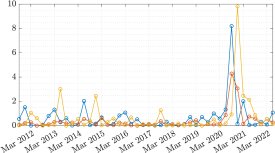
GDP	unemployment rate
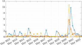
NFCI

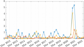
Figure 1: Quantile scores over time for the QVAR-SV model for GDP (top left), Unemployment rate (top right) and NFCI (bottom center), with different quantiles: $\tau=0.1$ (blue line); $\tau=0.5$ (red) and $\tau=0.9$ (yellow).

The quantile scores for the unemployment rate have an overall similar pattern over time, with some additional occasional falls of the performance for the $10$th percentile and smaller drops for the $90$th percentile before the outbreak of COVID-19. In particular, the left tail quantile shows a peak in the quantile score of about 3.0 in 2014:Q4 corresponding to one of the largest over-the-year decline since the end of the last recession, dropping 1.3 percentage points, to 5.7 percent in 2014:Q4. A second important peak of the QS (about 2.7) happened in 2017:Q2, in correspondence with the lowest unemployment rate since the fourth quarter of 2000, and it was twice as large as the 2016 decline. On the other hand, the QS for the right tail quantile witness lower peaks and its value overlaps with the left tail quantile during the first quarter of 2019. During this period, the US economy continued to expand, and the number of employed people increased by 2.0 million over the year, reaching 158.6 million in 2019:Q4. This growth was smaller than the over-the-year increase of 2.8 million in 2018, partly reflecting slower population growth. As stated for the GDP, the highest peaks in the QS occur during the COVID-19 pandemic, where the lock-downs in US increased the unemployment rate to 8.1 percent, close to value registered during the Great recession. Concerning the median, the QS is stable across time and during the COVID-19 pandemic provides evidence of small peaks.

Finally, the QS for the NFCI shows a sinusoidal trajectory for the $10$th percentile and lower peaks for the $90$th percentile. The strong increase in the QS during the COVID-19 pandemic previously described for macroeconomic variable is also witnessed for this financial variables, except for the median, which is rather flat. Moreover, in the left tail quantile, the periods between the second and last quarter of 2013, the last quarter of 2016 and the whole 2018 highlight important dynamics. These periods are strictly related to the US debt-ceiling crisis of 2013, and the 2015–2016 stock market selloff, which was characterized by a decline of the stock prices. Moreover it includes 2018, the worst year for stocks since the financial crisis since S&P 500 index finished the year down 6%, the Dow Jones Industrial Average dropped 5.6%, and the NASDAQ composite slid nearly 4%.

Overall, these findings support the claim that commonly-used approaches modeling the conditional mean and median are likely to miss meaningful changes of the macroeconomic and financial tail risks, thus supporting the use of a (multivariate) quantile regression framework.

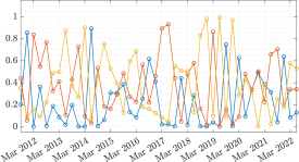
$\tau=0.1$	$\tau=0.5$
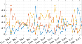
$\tau=0.9$

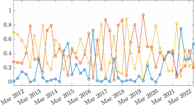
Figure 2: Time-varying combination weights for GDP for the QVAR-SV (red line); QVAR-GARCH (yellow) and QVAR (blue) with different quantiles: $\tau=0.1$ (top left), $\tau=0.5$ (top right) and $\tau=0.9$ (bottom center).

Figures 2 and 3 show the time-varying weights associated with the three QVAR models with constant volatility, stochastic volatility, and GARCH effects for the GDP and the NFCI, respectively. Figure 2 plots the results for three different quantiles: the $10$th, $50$th, and $90$th percentiles. First, we notice the large uncertainty on the weights, with substantial variation over time. Second, for the left and right quantile, we find evidence of an intense change of the relative performance of the different time-varying volatility specifications over time. Moreover, the constant volatility framework lags behind across all the quantiles and almost all periods considered, supporting the claim that, paralleling conditional mean models, time-varying volatility improves the forecasting performance for conditional quantiles. Finally, for the $10$th percentile, in 2012–2013 and 2018–2019, there is evidence of the importance of one time-varying volatility model, with weights around 90%. These patterns are less evident in the median quantile, while in the $90$th percentile is strong only in the period around 2017 and 2018. Conversely, we notice that since the outbreak of the COVID-19 pandemic, the relative performance of all the models seems to have leveled up, as the combination weights are evenly distributed.

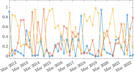
$\tau=0.1$	$\tau=0.5$
$\tau=0.9$

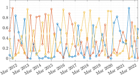
Figure 3: Time-varying combination weights for NFCI for the QVAR-SV (red line); QVAR-GARCH (yellow) and QVAR (blue) with different quantiles: $\tau=0.1$ (top left), $\tau=0.5$ (top right) and $\tau=0.9$ (bottom center).

Figure 3 reports the time-varying weights for the financial variable, NFCI. The homoskedastic QVAR model has almost zero weight for all the percentiles analyzed, except a few isolated spikes for the $10$th and $90$th percentile. Looking closer, the left quantile provides evidence that the QVAR-GARCH model is the best performing (in relative terms), except between 2014–2015, where the QVAR-SV model was the best. On the other hand, when investigating the right quantile models’ performances are less persistent across time, witnessing numerous switched between QVAR-SV and QVAR-GARCH. However, similarly to the left tail, the QVAR-SV model seems to be the best model from 2014 to 2015, while the QVAR-GARCH model has highest weights from 2018 to 2020. Regarding the median, there is evidence in favor of QVAR-GARCH effects, while the homoskedastic case is important only at the beginning of the out-of-sample.

Please refer to Section 2 for the details on models. All forecasts are produced with a one-step-ahead expanding window process.

^∗∗∗, ^∗∗ and ^∗ indicate that ratios are significantly different from 1 at $1\%$, $5\%$ and $10\%$, according to the Diebold-Mariano test.

Bold numbers indicate models that belong to the Superior Set of Models delivered by the MCS procedure at confidence level $10\%$.

Table 2: Quantile Score for different variables (columns) and percentiles ($\tau=0.1,0.3,0.5,0.7$ and $0.9$).

Variable	AWHMAN	CPIAUCSL	INDPRO	S&P500	FEDFUNDS	GS10	UNRATE	NFCI	GDPC1
Quantile: $\tau=0.1$
QVAR	1.699	1.128	1.598	1.806	1.855	2.078	1.901	1.497	1.793
QVAR-SV	0.601∗∗∗	0.568∗∗	0.627∗∗∗	0.425∗∗∗	0.618∗∗∗	0.591∗∗∗	0.963∗∗∗	0.643∗∗∗	0.643∗∗∗
QVAR-GARCH	1.091	0.476∗∗∗	0.932	0.523∗∗∗	0.347∗∗∗	0.570∗∗∗	1.126∗	0.349∗∗∗	0.974∗
QVAR Combination (AVG)	1.136∗∗	0.538∗∗∗	0.731∗∗∗	0.512∗∗∗	0.482∗∗∗	0.574∗∗∗	1.050∗∗	0.450∗∗∗	0.828∗∗∗
QVAR Combination (T-V)	0.360∗∗∗	1.100	0.511∗∗∗	0.415∗∗∗	0.480∗∗∗	0.463∗∗∗	0.581∗∗∗	0.591∗∗∗	0.480∗∗∗
QAR	1.763	1.869	1.728	1.514	1.277	1.732	1.937	1.604	1.788
QAR-SV	1.721	2.261	1.643	1.933	1.950	1.864	1.979	2.315	1.836
QAR-GARCH	2.054	2.562	2.279	2.370	1.754	2.242	1.953	1.651	2.163
QAR Combination (AVG)	1.792	2.224	1.690	1.673	1.441	2.048	1.937	1.843	1.886
QAR Combination (T-V)	1.705	1.974	1.565	0.997∗∗∗	0.905∗∗∗	0.758∗∗∗	0.841∗∗∗	0.657∗∗∗	0.405∗∗∗
Quantile: $\tau=0.3$
QVAR	0.579	0.634	0.551	0.701	0.436	0.744	0.841	0.426	0.760
QVAR-SV	0.393∗∗	0.410∗∗∗	0.368∗∗∗	0.321∗∗∗	0.266∗∗∗	0.443∗∗∗	0.645∗∗	0.361	0.426∗∗∗
QVAR-GARCH	0.659	0.416∗∗∗	0.755	0.472	0.220∗∗∗	0.677	0.565∗∗∗	0.228∗∗∗	0.694
QVAR Combination (AVG)	0.396∗∗∗	0.412∗∗∗	0.395∗∗∗	0.449∗	0.220∗∗∗	0.544∗	0.601∗∗∗	0.247∗∗∗	0.438∗∗∗
QVAR Combination (T-V)	0.630	0.784	0.422∗	0.338∗∗∗	0.352	0.383∗∗∗	0.514∗∗∗	0.479	0.407∗∗∗
QAR	0.771	0.794	0.682	0.530	0.522	0.667	0.989	0.642	0.731
QAR-SV	0.785	0.857	0.816	0.700	0.667	0.776	0.950	0.928	0.777
QAR-GARCH	0.828	0.909	1.076	0.793	0.606	0.910	1.010	0.628	0.994
QAR Combination (AVG)	0.768	0.854	0.800	0.649	0.601	0.693	0.958	0.688	0.743
QAR Combination (T-V)	1.402	1.542	1.168	0.818	0.721	0.601	0.708∗∗∗	0.511∗∗∗	0.373∗∗∗
Quantile: $\tau=0.5$
QVAR	0.510	0.403	0.506	0.403	0.323	0.472	0.725	0.325	0.508
QAR-SV	0.389∗∗∗	0.279∗∗∗	0.383∗∗	0.313∗	0.173∗∗∗	0.312∗∗∗	0.446∗∗∗	0.180∗∗∗	0.383∗∗∗
QAR-GARCH	0.340∗∗∗	0.273∗∗∗	0.368∗∗	0.293∗∗	0.151∗∗∗	0.274∗∗∗	0.357∗∗∗	0.123∗∗∗	0.363∗∗∗
QVAR Combination (AVG)	0.384∗∗∗	0.273∗∗∗	0.370∗∗∗	0.330∗∗	0.148∗∗∗	0.285∗∗∗	0.389∗∗∗	0.175∗∗∗	0.359∗∗∗
QVAR Combination (T-V)	0.623	0.624	0.393∗∗	0.387	0.248	0.313∗	0.458∗∗∗	0.341	0.376∗∗∗
QAR	0.336	0.285	0.339	0.294	0.234	0.249	0.410	0.103	0.365
QAR-SV	0.338	0.285	0.331	0.276	0.263	0.263	0.388∗	0.173	0.353
QAR-GARCH	0.328	0.280	0.331	0.286	0.095∗∗∗	0.264	0.380∗∗	0.076∗∗	0.337∗
QAR Combination (AVG)	0.334	0.278	0.325	0.282∗	0.194∗∗	0.252	0.379∗∗	0.091	0.340∗∗
QAR Combination (T-V)	1.010	1.127	0.871	0.572	0.502	0.428	0.588	0.358	0.345
Quantile: $\tau=0.7$
QVAR	0.578	0.530	0.526	0.755	0.569	0.688	0.739	0.414	0.613
QVAR-SV	0.473∗∗	0.389∗∗∗	0.426∗∗	0.469∗∗∗	0.306∗∗∗	0.416∗∗∗	0.380∗∗∗	0.265∗∗	0.449∗∗
QVAR-GARCH	0.471∗	0.317∗∗∗	0.520	0.506∗∗∗	0.239∗∗∗	0.362∗∗∗	1.047	0.266	0.688
QVAR Combination (AVG)	0.482∗∗∗	0.374∗∗∗	0.459	0.548∗∗∗	0.383∗∗∗	0.414∗∗∗	0.608	0.252∗	0.564
QVAR Combination (T-V)	0.451	0.408∗∗	0.246∗∗	0.375∗∗∗	0.226∗∗∗	0.272∗∗∗	0.375∗∗∗	0.219∗∗∗	0.344∗∗∗
QAR	0.770	0.588	0.679	0.809	0.483	0.650	0.559	0.400	0.774
QAR-SV	0.803	0.684	0.807	0.875	0.757	0.709	0.574	0.611	0.806
QAR-GARCH	0.971	0.511∗	0.869	0.948	0.375∗∗∗	0.734	0.664	0.178∗∗∗	0.875
QAR Combination (AVG)	0.834	0.557	0.708	0.932	0.468	0.698	0.577	0.335∗∗∗	0.817
QAR Combination (T-V)	0.604	0.675	0.503	0.351∗∗∗	0.391	0.284∗∗∗	0.447∗∗	0.228∗∗∗	0.313∗∗∗
Quantile: $\tau=0.9$
QVAR	2.115	1.822	1.804	2.050	1.618	1.853	1.881	1.180	1.814
QVAR-SV	0.665∗∗∗	0.488∗∗∗	0.553∗∗∗	0.754∗∗∗	0.417∗∗∗	0.526∗∗∗	0.616∗∗∗	0.344∗∗∗	0.684∗∗∗
QVAR-GARCH	0.725∗∗∗	0.396∗∗∗	0.696∗∗∗	0.893∗∗∗	0.564∗∗∗	0.587∗∗∗	1.892	0.564∗	1.022∗
QVAR Combination (AVG)	0.717∗∗∗	1.492∗∗∗	1.207∗∗∗	0.759∗∗∗	0.484∗∗∗	0.515∗∗∗	1.364	0.568∗∗	0.792∗∗∗
QVAR Combination (T-V)	0.238∗∗∗	0.187∗∗∗	0.147∗∗∗	0.304∗∗∗	0.140∗∗∗	0.198∗∗∗	0.322∗∗∗	0.111∗∗∗	0.315∗∗∗
QAR	1.745	1.415	1.666	1.815	1.370	1.518	1.667	1.319	1.734
QAR-SV	1.964	1.911	1.980	1.911	1.502	1.792	1.407∗∗	1.647	1.939
QAR-GARCH	2.205	1.099∗∗	2.012	2.356	1.558	1.842	1.608	0.832∗∗∗	1.751
QAR Combination (AVG)	1.917	1.218∗∗	1.915	1.906	1.466	1.696	1.519∗	1.519	1.810
QAR Combination (T-V)	0.203∗∗∗	0.225∗∗∗	0.170∗∗∗	0.115∗∗∗	0.105∗∗∗	0.127∗∗∗	0.318∗∗∗	0.077∗∗∗	0.277∗∗∗

Moving to the forecasting exercise, we have compared the QVAR model with $1$ lag and different time-varying volatility for various quantile levels $\tau\in\{0.1,0.2,\ldots,0.9\}$ by using an expanding window approach. Besides the multivariate models, we have also considered the univariate model specification for the QAR, QAR-SV and QAR-GARCH model. For completeness, we have included in the table the forecast combination with time-varying weights and as weighted average for the multivariate and univariate model.

Table LABEL:tab:Result_expanding shows the results of the forecasting exercise across variables (in column) for five quantile levels, $\tau\in\{0.1,0.3,0.5,0.7,0.9\}$, using an expanding window approach. It also reports the outcome of the Diebold-Mariano (DM) test against the benchmark (the univariate and multivariate quantile VAR with constant volatility) and the model confidence set at $10\%$ with respect to all the models.

In line with the previously commented graphical inspection, Table LABEL:tab:Result_expanding provides evidence supporting the variation of the models’ forecasting performance across the variable of interest and the quantile investigated. At the $10$th percentile, there is evidence of better forecasting results from QVAR models, for each variable, and this is confirmed by the model confidence set. Moreover, for inflation, federal reserve funds, and NFCI, the best model is the QVAR-GARCH, whereas for the other variables the combination of multivariate models yields more promising forecasts. These results are also confirmed by the Diebold-Mariano test, which highlights a significant difference in the performance of models with time-varying volatility compared to the homoskedastic benchmark. Finally, the Diebold-Mariano test and the model confidence set suggest that the most suitable model for the left tail ($10$th percentile) is the (multivariate) model combination obtained using time-varying weights. Concerning the $30$th percentile, the QVAR-SV is the best model for inflation, average weekly hours, and industrial production. On the other hand, for better forecasts of the unemployment rate and the GDP are obtained using a combination of multivariate QVAR models.

In terms of the median ($\tau=0.5$), the model confidence set shows no strong evidence in favor of the inclusion of time-varying volatility, however the DM test indicates that QVAR models with either stochastic volatility or GARCH statistically outperform the benchmark at the $10\%$ level. Regarding the right tail at the $70$th percentile, we find strong evidence in favor of time-varying volatility models and the model combination. Overall, including SV and GARCH improves the QVAR performance across all the variables, according to both the model confidence set and the DM test. In more details, when forecasting inflation and NFCI, including GARCH specification leads to improvements in both multivariate and univariate models. Moreover, using a combination of multivariate models with constant weights improves the performance for almost all the variables, except S&P 500 and GDP, where the differences in favor of univariate combination are smaller with respect to the multivariate specification. At the $90$th percentile, the results provide strong evidence supporting the inclusion of time-varying volatility in multivariate models. In particular, the QVAR-SV model yields better performances for almost all the variables, except inflation. However, the best specification for all variables is the univariate model combination with time-varying weights, whereas the same combination of multivariate specifications has slighlty worse performance despite belonging to the model confidence set in most of the cases.

Overall, these results highlight that accounting for time-varying volatility in its different specifications improves forecast accuracy, both using univariate and multivariate settings, especially when investigating the tails. Moreover, the multivariate framework provide better performances overall, with the multivariate model combination obtained using time-varying weights appearing as the most accurate in many quantile/variable settings. Conversely, when modeling the median, these improvements are less remarkable and have lower statistical significance. This suggests that, when a forecaster is concerned with predicting the tail behavior of a variable, accounting for time-varying is crucial to obtain more reliable results.

5 Conclusions

Motivated by the increasing interest of central bankers, researchers and policy institutions in tail risk evaluation and forecasting, we extended the multivariate quantile regression framework to account for alternative time-varying volatility specification, through stochastic volatility or GARCH effects. These models have been complemented by a model combination that exploits the quantile score to define the (possibly time-varying) weights. To make inference on the latent volatility paths, we designed an efficient MCMC algorithm that allows us to sample the entire path of the series-specific time-varying volatility jointly and independently across equations, allowing for meaningful computational savings.

We applied the proposed methods in multivariate and univariate formulation to forecast US macroeconomic and financial data at several quantile levels. The main findings highlight that including time-varying volatility significantly improves the forecasting performance in all cases, especially on the tails of the distribution. Moreover, as no single model is found to besupeiror than others across quantiles or variables, we propose a multivariate model combination with time-varying weighting scheme.

References

- Aastveit et al. (2022) Aastveit, K. A., S. ter Ellen, and G. Mantoan (2022). Quantile density combination: An application to US GDP forecasts. Technical report.
- Adams et al. (2021) Adams, P. A., T. Adrian, N. Boyarchenko, and D. Giannone (2021). Forecasting macroeconomic risks. International Journal of Forecasting 37(3), 1173–1191.
- Adrian et al. (2019) Adrian, T., N. Boyarchenko, and D. Giannone (2019). Vulnerable growth. American Economic Review 109(4), 1263–89.
- Adrian et al. (2022) Adrian, T., F. Grinberg, N. Liang, S. Malik, and J. Yu (2022). The term structure of growth-at-risk. American Economic Journal: Macroeconomics 14(3), 283–323.
- Atchadé and Rosenthal (2005) Atchadé, Y. F. and J. S. Rosenthal (2005). On adaptive Markov chain Monte Carlo algorithms. Bernoulli 11(5), 815–828.
- Bollerslev (1986) Bollerslev, T. (1986). Generalized autoregressive conditional heteroskedasticity. Journal of Econometrics 31(3), 307–327.
- Caporin et al. (2021) Caporin, M., R. Gupta, and F. Ravazzolo (2021). Contagion between real estate and financial markets: A bayesian quantile-on-quantile approach. The North American Journal of Economics and Finance 55, 101347.
- Caporin et al. (2018) Caporin, M., L. Pelizzon, F. Ravazzolo, and R. Rigobon (2018). Measuring sovereign contagion in europe. Journal of Financial Stability 34, 150–181.
- Carriero et al. (2016) Carriero, A., T. E. Clark, and M. Marcellino (2016). Common Drifting Volatility in Large Bayesian VARs. Journal of Business & Economic Statistics 34(3), 375–390.
- Carriero et al. (2022) Carriero, A., T. E. Clark, and M. Marcellino (2022). Nowcasting tail risk to economic activity at a weekly frequency. Journal of Applied Econometrics 37(5), 843–866.
- Chavleishvili and Manganelli (2021) Chavleishvili, S. and S. Manganelli (2021). Forecasting and Stress Testing with Quantile Vector Autoregression. Technical Report 2330, ECB Working Paper.
- Clark and Ravazzolo (2015) Clark, T. E. and F. Ravazzolo (2015). Macroeconomic Forecasting Performance under Alternative Specifications of Time-Varying Volatility. Journal of Applied Econometrics 30(4), 551–575.
- Cogley and Sargent (2005) Cogley, T. and T. J. Sargent (2005). Drifts and volatilities: monetary policies and outcomes in the post WWII US. Review of Economic dynamics 8(2), 262–302.
- Cox et al. (1981) Cox, D. R., G. Gudmundsson, G. Lindgren, L. Bondesson, E. Harsaae, P. Laake, K. Juselius, and S. L. Lauritzen (1981). Statistical analysis of time series: Some recent developments [with discussion and reply]. Scandinavian Journal of Statistics, 93–115.
- Cross et al. (2021) Cross, J. L., C. Hou, G. Koop, and A. Poon (2021). Macroeconomic Forecasting with Large Stochastic Volatility in Mean VARs.
- D’Agostino et al. (2013) D’Agostino, A., L. Gambetti, and D. Giannone (2013). Macroeconomic forecasting and structural change. Journal of Applied Econometrics 28(1), 82–101.
- Diebold and Mariano (1995) Diebold, F. and R. Mariano (1995). Comparing predictive accuracy. Journal of Business and Economic Statistics 13(3), 253–263.
- Engle (1982) Engle, R. F. (1982). Autoregressive Conditional Heteroscedasticity with Estimates of the Variance of United Kingdom Inflation. Econometrica 50(4), 987–1007.
- Ferrara et al. (2022) Ferrara, L., M. Mogliani, and J.-G. Sahuc (2022). High-frequency monitoring of growth at risk. International Journal of Forecasting 38(2), 582–595.
- Giacomini and Komunjer (2005) Giacomini, R. and I. Komunjer (2005). Evaluation and combination of conditional quantile forecasts. Journal of Business & Economic Statistics 23(4), 416–431.
- Hansen et al. (2011) Hansen, P. R., A. Lunde, and J. M. Nason (2011). The Model Confidence Set. Econometrica 79, 453–497.
- Iacopini et al. (2022) Iacopini, M., A. Poon, L. Rossini, and D. Zhu (2022). Bayesian Mixed-Frequency Quantile Vector Autoregression: Eliciting tail risks of Monthly US GDP. Technical report, arXiv.
- Kastner and Frühwirth-Schnatter (2014) Kastner, G. and S. Frühwirth-Schnatter (2014). Ancillarity-sufficiency interweaving strategy (ASIS) for boosting MCMC estimation of stochastic volatility models. Computational Statistics & Data Analysis 76, 408–423.
- Koenker and Bassett (1978) Koenker, R. and G. Bassett (1978). Regression quantiles. Econometrica, 33–50.
- Kotz et al. (2001) Kotz, S., T. Kozubowski, and K. Podgórski (2001). The Laplace distribution and generalizations: a revisit with applications to communications, economics, engineering, and finance. Number 183. Springer Science & Business Media.
- Kozumi and Kobayashi (2011) Kozumi, H. and G. Kobayashi (2011). Gibbs sampling methods for Bayesian quantile regression. Journal of Statistical Computation and Simulation 81(11), 1565–1578.
- Marcellino et al. (2016) Marcellino, M., M. Porqueddu, and F. Venditti (2016). Short-term gdp forecasting with a mixed-frequency dynamic factor model with stochastic volatility. Journal of Business & Economic Statistics 34(1), 118–127.
- Petrella and Raponi (2019) Petrella, L. and V. Raponi (2019). Joint estimation of conditional quantiles in multivariate linear regression models with an application to financial distress. Journal of Multivariate Analysis 173, 70–84.
- Pfarrhofer (2022) Pfarrhofer, M. (2022). Modeling tail risks of inflation using unobserved component quantile regressions. Journal of Economic Dynamics and Control 143, 104493.
- Primiceri (2005) Primiceri, G. E. (2005, 07). Time Varying Structural Vector Autoregressions and Monetary Policy. The Review of Economic Studies 72(3), 821–852.
- Taylor (1986) Taylor, S. J. (1986). Modelling financial time series. Wiley.
- Xiao (2017) Xiao, Z. (2017). Qar and quantile time series analysis. In Handbook of quantile regression, pp. 293–332. Chapman and Hall/CRC.