A group action on higher Chow cycles on a family of Kummer surfaces

Abstract.

We construct a family of Kummer surfaces ${\mathcal{X}}^{\circ}\rightarrow T^{\circ}$ from the Legendre family of elliptic curves. Then we construct a family of higher Chow cycles on ${\mathcal{X}}^{\circ}\rightarrow T^{\circ}$ and calculate their values under the transcendental regulator map. For the calculation, we use a finite group action on ${\mathcal{X}}^{\circ}\rightarrow T^{\circ}$. We show that the rank of the space of the indecomposable cycles of ${\mathcal{X}}_{t}$ is greater than or equal to $18$ for very general $t\in T^{\circ}({\mathbb{C}})$. To show the linearly independence of indecomposable higher Chow cycles, we consider the image of normal functions associated to higher Chow cycles under a Picard-Fuchs differential operator of ${\mathcal{X}}^{\circ}\rightarrow T^{\circ}$.

1. Introduction

1.1. Contents of this paper

In the celebrated paper [Blo86], Bloch defined higher Chow groups ${\mathrm{CH}}^{p}(X,q)$ for a variety $X$ over a field $k$. Higher Chow groups are a natural generalization of Chow groups. For a closed subvariety $Z\subset X$ of codimension $c$, the localization exact sequence of Chow groups

$${\mathrm{CH}}^{p-c}(Z)\rightarrow{\mathrm{CH}}^{p}(X)\rightarrow{\mathrm{CH}}^{p}(X-Z)\rightarrow 0$$

fits into the localization exact sequence of higher Chow groups

$$\cdots\rightarrow{\mathrm{CH}}^{p}(X,1)\rightarrow{\mathrm{CH}}^{p}(X-Z,1)\rightarrow{\mathrm{CH}}^{p-c}(Z)\rightarrow{\mathrm{CH}}^{p}(X)\rightarrow{\mathrm{CH}}^{p}(X-Z)\rightarrow 0.$$ (1)

Thus higher Chow groups are an analogue of the singular cohomologies for algebraic varieties. Furthermore, there exists a canonical isomorphism

$${\mathrm{CH}}^{p}(X,q)\otimes_{{\mathbb{Z}}}{\mathbb{Q}}\simeq H^{2p-q}_{\mathcal{M}}(X,{\mathbb{Q}}(p))$$ (2)

where $H^{2p-q}_{\mathcal{M}}(X,{\mathbb{Q}}(p))$ is the motivic cohomology of $X$. Motivic cohomologies and higher Chow groups appear in many aspects of algebraic geometry and number theory. However, its structure is still mysterious for many varieties.

In this paper, we study higher Chow cycles in ${\mathrm{CH}}^{2}(X,1)$ for a certain type of $K3$ surfaces, which are regarded as 2-dimensional analogues of elliptic curves. Higher Chow groups of general $K3$ surfaces are studied in [CDKL16]. We treat a special type of Kummer surfaces and study their higher Chow groups in detail.

We consider the following map induced by the intersection product.

$${\mathrm{CH}}^{1}(X,1)\otimes_{\mathbb{Z}}{\mathrm{CH}}^{1}(X)\>{\longrightarrow}\>{\mathrm{CH}}^{2}(X,1)$$ (3)

Since ${\mathrm{CH}}^{1}(X)\simeq\mathrm{Pic}(X)$ and ${\mathrm{CH}}^{1}(X,1)\simeq\Gamma(X,{\mathcal{O}}_{X}^{\times})$, the image of (3) can be described by the known invariants. Hence we are interested in the cokernel ${\mathrm{CH}}^{2}(X,1)_{\mathrm{ind}}$ of (3), which is called the indecomposable part of ${\mathrm{CH}}^{2}(X,1)$. In this paper, we give an estimate for the rank of ${\mathrm{CH}}^{2}(X,1)_{\mathrm{ind}}$.

For the estimation, we construct elements in ${\mathrm{CH}}^{2}(X,1)$ explicitly, and consider their images under the following regulator map defined by Beilinson.

(4)

Here the target $H^{3}_{\mathcal{D}}(X,{\mathbb{Q}}(2))$ is the Deligne cohomology of $X$. In the articles [GL99],[Mül97], [CDKL16], [dAM02],[Col97] and [Asa16], they consider families of varieties $\{X_{t}\}_{t\in T}$ and construct families of higher Chow cycles $\{\xi_{t}\}_{t\in T}$. Then they show that $\xi_{t}$ does not vanish for very general $t\in T$ by studying the behavior of the images of these cycles under the regulator map as a function of $t$. We follow this strategy.

In this paper, we consider a family of Kummer surfaces ${\mathcal{X}}^{\circ}\rightarrow T^{\circ}$, which is constructed in Section 3. We construct a family of higher Chow subgroups $\Xi=\{\Xi_{t}\subset{\mathrm{CH}}^{2}({\mathcal{X}}_{t},1)\}_{t\in T^{\circ}}$ and compute their images under the following transcendental regulator maps $r$ at fibers.

(5)

Here the upper left map is the regulator map. The transcendental regulator map factors through ${\mathrm{CH}}^{2}({\mathcal{X}}_{t},1)_{\mathrm{ind}}$. Thus we can use the transcendental regulator map for the rank estimate for indecomposable parts. The main theorem of this paper is as follows.

Theorem 1.1.

$(\mathrm{Theorem}$ $\ref{mainthmpart3})$ For a very general $t\in T^{\circ}({\mathbb{C}})$,

$${\mathrm{rank}\>}r(\Xi_{t})=18.$$ (6)

Especially, ${\mathrm{rank}\>}{\mathrm{CH}}^{2}({\mathcal{X}}_{t},1)_{\mathrm{ind}}\geq 18$.

Since ${\mathcal{X}}^{\circ}\rightarrow T^{\circ}$ is a certain base change of the Kummer surface family treated in Section 6 of [CDKL16], ${\mathrm{CH}}^{2}({\mathcal{X}}_{t},1)_{\mathrm{ind}}\neq 0$ was already known for very general $t$. Theorem 1.1 improves the estimate for the rank of ${\mathrm{CH}}^{2}({\mathcal{X}}_{t},1)_{\mathrm{ind}}$. While the construction of a higher Chow cycle in [CDKL16] is based on a certain elliptic fibration structure of ${\mathcal{X}}_{t}$, our construction of $\Xi_{t}$ is based on the fact that ${\mathcal{X}}_{t}$ is the minimal desingularization of a double covering of ${\mathbb{P}}^{1}_{k}\times_{k}{\mathbb{P}}^{1}_{k}$. Thus we give a new way of construction of higher Chow cycles on such type of Kummer surfaces in this paper. The merit of our construction is that the values of the transcendental regulator maps can be represented by relatively simple integrals. e.g. (7)

For the computation of the image of the transcendental regulator map, we construct topological chains on ${\mathcal{X}}_{t}^{\mathrm{an}}$ explicitly (Section 8) and use the formula obtained by Levine ([Lev88]). By Levine’s formula, the following multivalued holomorphic function appears in the image of an element of $\Xi$ under the transcendental regulator map (Proposition 8.10).

$${\mathcal{L}}(a,b)=\int_{\triangle}\frac{dxdy}{\sqrt{x(1-x)(1-ax)}\sqrt{y(1-y)(1-by)}}$$ (7)

Here $\triangle=\{(x,y)\in{\mathbb{R}}^{2}\>:\>0<y<x<1\}$. (7) is similar to the integral representation of Appell’s hypergeometric functions. A difference is that the boundary of the domain of integral is not necessarily contained in the branching locus of the integrand. In other words, (7) is a kind of incomplete integrals.

The Beilinson conjecture predicts that if $X$ is defined over a number field, the values (in a suitable sense) of the regulator map (4) are related to the special values of $L$-functions of motives of $X$. Hence it is an interesting problem what kinds of functions appear in the image of the regulator map.

Recently, in [AO18], Asakura and Otsubo gives examples of special varieties (which have hypergeometric fibrations) whose values of the regulator maps are represented by the value at $z=1$ of a generalized hypergeometric function ${}_{3}F_{2}$. Furthermore, by deforming such varieties, they give a 1-dimensional family of varieties such that the value of the regulator map of members of such family is represented by generalized hypergeometric function ${}_{3}F_{2}$ ([AO21]). Hence some relations between the value of the regulator map and hypergeometric functions were known. The object we treat in this paper can be regarded as a certain ${\mathbb{Q}}^{\oplus 18}$-extension of the exterior tensor product of two Gauss hypergeometric differential equations ${}_{2}F_{1}$.

To compute the value of transcendental regulator for each element in $\Xi$, we use automorphisms of the Kummer surface family. We consider the following type of automorphisms of a family of algebraic varieties.

Definition 1.2.

Let $X\rightarrow S$ be a family of algebraic varieties over a field $k$. The automorphism group ${\mathrm{Aut}}_{k}(X\rightarrow S)$ of $X\rightarrow S$ consists of a pair $(g,\underline{g})$ with $g\in{\mathrm{Aut}}_{k}(X)$ and $\underline{g}\in{\mathrm{Aut}}_{k}(S)$ such that the following diagram commutes.

(8)

In this paper, we construct the following finite group action explicitly on the Kummer surface family ${\mathcal{X}}^{\circ}\rightarrow T^{\circ}$. Let $V$ be the Klein four-group and $\pi$ be the natural projection $\mathfrak{S}_{4}\rightarrow{\mathfrak{S}}_{4}/V={\mathfrak{S}}_{3}$. We set $G=(\{(h_{1},h_{2})\in\mathfrak{S}_{4}\times\mathfrak{S}_{4}:\pi(h_{1})=\pi(h_{2})\})^{2}$. We define a ${\mathbb{Z}}/2{\mathbb{Z}}$-extension $\widetilde{G}$ of $G$ (Definition 4.17).

Proposition 1.3.

$(\mathrm{Proposition}$ $\ref{mainprop1})$ The group $\widetilde{G}$ acts faithfully on the family ${\mathcal{X}}^{\circ}\rightarrow T^{\circ}$.

Then we construct a subgroup $\Xi^{\mathrm{can}}\subset{\mathrm{CH}}^{2}({\mathcal{X}}^{\circ},1)$ and define $\Xi$ as the sum of $\widetilde{\rho}_{*}\Xi^{\mathrm{can}}\>(\widetilde{\rho}\in\widetilde{G})$. The author is informed of the constructions of several elements in $\Xi$ by Terasoma in seminars. We generalize his idea of the constructions of higher Chow cycles so that we can use automorphisms of ${\mathcal{X}}^{\circ}\rightarrow T^{\circ}$.

We compute the image of $\Xi$ under the regulator map by using $\widetilde{G}$-action as follows: since $\Xi$ is constructed as a family over $T^{\circ}$, we can define a “relative transcendental regulator map” $R_{\omega}$ (Definition 9.11)

(9)

where ${\mathcal{Q}}_{\omega}$ is a sheaf on $(T^{\circ})^{\mathrm{an}}$ such that restriction of ${\mathcal{Q}}_{\omega}$ at $t\in T^{\circ}({\mathbb{C}})$ is isomorphic to $(H^{2,0}({\mathcal{X}}_{t}^{\mathrm{an}}))^{\vee}/H_{2}({\mathcal{X}}_{t}^{\mathrm{an}},{\mathbb{Q}})$. The reason why $R_{\omega}$ is called “relative transcendental regulator” is that the restriction of $R_{\omega}(\Xi)$ at $t\in T^{\circ}({\mathbb{C}})$ coincides with $r(\Xi_{t})$ modulo torsion part. This relative transcendental regulator map associates families of higher Chow cycles to (a generalization of) normal functions. Though this kind of maps can be defined in more general setting (cf.[Sai02] and [CDKL16]), we employ an ad hoc definition since we need only the explicit description for special cases.

We define a $\widetilde{G}$-action on ${\mathcal{Q}}_{\omega}$ so that $R_{\omega}$ is equivariant under this action. Thus we reduce the computation of $r(\Xi_{t})$ to that of $R_{\omega}(\Xi)$ and the $\widetilde{G}$-action on ${\mathcal{Q}}_{\omega}(T^{\circ})$. In Section 6, we construct two subgroups $\widetilde{I}\simeq(\mathfrak{S}_{4}\times_{\mathfrak{S}_{3}}\mathfrak{S}_{4})\times({\mathbb{Z}}/2{\mathbb{Z}})$ and $\widetilde{G}_{\mathrm{fib}}\simeq({\mathbb{Z}}/2{\mathbb{Z}})^{5}$ of $\widetilde{G}$ which stabilize $R_{\omega}(\Xi^{\mathrm{can}})\subset{\mathcal{Q}}_{\omega}(T^{\circ})$. Since $\Xi$ is defined as the sum of $\widetilde{\rho}_{*}\Xi^{\mathrm{can}}$, we can show that the rank of $R_{\omega}(\Xi)$ is at most 18 by examining the size of the stabilizer of $R_{\omega}(\Xi^{\mathrm{can}})$.

To show that the rank of $R_{\omega}(\Xi)$ is exactly 18, we consider the image of $R_{\omega}(\Xi)\subset{\mathcal{Q}}_{\omega}(T^{\circ})$ under a Picard-Fuchs differential operator

(10)

Similar methods are used in [Mül97], [dAM02] and [CDKL16]. We define a $\widetilde{G}$-action on ${\mathcal{O}}(T^{\circ})^{\oplus 2}$ so that ${\mathscr{D}}$ is $\widetilde{G}$-equivariant. To prove the equivariance, we show the transformation formulae of Picard-Fuchs differential operators by $\widetilde{G}$-action (Proposition 9.18). This result is interesting by itself from the point of view of differential equations. Using a simple description of ${\mathscr{D}}\circ R_{\omega}(\Xi)$, we show that ${\mathscr{D}}\circ R_{\omega}(\Xi)$ has 18 ${\mathbb{Q}}$-linearly independent elements (Table 8). Thus we can show Theorem 1.1.

1.2. Outline of this paper

This paper is divided into 3 parts.

Part 1 consists of Section 2, Section 3 and Section 4. The purpose of Part 1 is to fix the notation and to prove Proposition 1.3. In Section 2, we introduce a category ${\mathrm{(Sch}^{\mathrm{gp}}/k)}$, which is used to consider multiple finite group actions on multiple schemes simultaneously. In Section 3, we construct the Kummer surface family ${\mathcal{X}}\rightarrow T$. In Section 4, we prove Proposition 1.3.

Part 2 consists of Section 5 and Section 6. The purpose of Part 2 is to explain the construction of $\Xi\subset{\mathrm{CH}}^{2}({\mathcal{X}}^{\circ},1)$ and consider the $\widetilde{G}$-action on $\Xi$. In Section 5, we first construct a subgroup of the higher Chow group $\Xi^{\mathrm{can}}\subset{\mathrm{CH}}^{2}({\mathcal{X}}^{\circ},1)$ and define $\Xi$ as the sum of its images under $\widetilde{G}$-action. In Section 6, we construct two subgroups $\widetilde{I}$ and $\widetilde{G}_{\mathrm{fib}}$ which stabilize the image of $\Xi^{\mathrm{can}}$ under the transcendental regulator map.

The purpose of Part 3 is to prove Theorem 1.1. Part 3 consists of Section 7, Section 8 and Section 9. In Section 7, we fix relative differential forms $\omega$ on ${\mathcal{X}}^{\circ}\rightarrow T^{\circ}$ and examine $\widetilde{G}$-action on $\omega$. Furthermore, we find a Picard-Fuchs differential operator ${\mathscr{D}}$ which annihilates period functions of ${\mathcal{X}}^{\circ}\rightarrow T^{\circ}$. In Section 8, we calculate the image of an element of $\Xi^{\mathrm{can}}_{t}$ under the transcendental regulator map. In Section 9, we define the relative transcendental regulator map $R_{\omega}$ in (9) and prove $\widetilde{G}$-equivariance of ${\mathscr{D}}$ and $R_{\omega}$. Finally, we prove Theorem 1.1.

In Appendix A, we recall the definition of decomposable cycles in higher Chow groups and how decomposable cycles are represented by elements of the homology group of the Gersten complex (cf. Proposition 5.1).

1.3. Acknowledgement

The author expresses his sincere gratitudes to his supervisor Professor Tomohide Terasoma, who gave the author the idea of the construction of higher Chow cycles in Section 5 and also the idea of the construction of the topological 2-chains in Section 8 and let the author know a technique of checking the non-triviality of higher Chow cycles as in [Mül97]. Furthermore, he gave the author many valuable comments which simplifies the arguments in this paper. He thanks Professor Shuji Saito sincerely, who gave the author many helpful comments on this paper and encouraged him during the doctoral course. He is also very grateful to Professor Takeshi Saito, who simplified the proof of Proposition 9.12 and improved sentences in the draft. The author is supported by the FMSP program by the University of Tokyo.

1.4. Conventions

1.4.1. Conventions for algebraic geometry

1. For a field $k$, a variety over $k$ is an integral separated scheme of finite type over $k$. For a variety $X$, its function field of $X$ is denoted by $R(X)$.

2. For a morphism $X\rightarrow S$ and $s\in S$, we usually denote the fiber over $s$ by $X_{s}$. For $\varphi\in{\mathrm{Hom}}_{S}(Y,X)$, $\varphi^{\sharp}$ denotes the morphism of sheaves of rings $\varphi^{\sharp}:{\mathcal{O}}_{X}\rightarrow\varphi_{*}{\mathcal{O}}_{Y}$.

3. For $S$-schemes $Y$ and $X$, ${\mathrm{Hom}}_{S}(Y,X)$ denotes the set of $S$-morphisms. If $Y={\mathrm{Spec}\,}R$, elements in ${\mathrm{Hom}}_{S}(Y,X)$ are called $R$-rational points and we also use the notation $X(R)$ for ${\mathrm{Hom}}_{S}(Y,X)$. The group of $S$-automorphisms of $X$ is denoted by ${\mathrm{Aut}}_{S}(X)$. For any morphism $S^{\prime}\rightarrow S$, we have a natural map ${\mathrm{Hom}}_{S}(Y,X)\rightarrow{\mathrm{Hom}}_{S^{\prime}}(Y\times_{S}S^{\prime},X\times_{S}S^{\prime})$. For a subset $\Sigma$ of ${\mathrm{Hom}}_{S}(Y,X)$, the image of $\Sigma$ under this map is called the base change of $\Sigma$ by $S^{\prime}\rightarrow S$.

4. For closed subschemes $Y_{1}$ and $Y_{2}$ of $X$ which satisfy $Y_{1}\cap Y_{2}=\emptyset$, $Y_{1}\sqcup Y_{2}\subset X$ denotes the closed subscheme corresponding to the ideal sheaf ${\mathcal{I}}_{Y_{1}}\cap{\mathcal{I}}_{Y_{2}}$ where ${\mathcal{I}}_{Y_{i}}$ is the ideal sheaf corresponding to $Y_{i}$.

1.4.2. Conventions for group theory

1. In this paper, we always consider left group actions. For a group $G$, the opposite $G$-action is a (left) action of the opposite group $G^{\mathrm{op}}$. Let $G$ be a group and $M$ be an abelian group with a $G$-action. For a subgroup $N\subset M$, the $G$-action of $M$ stabilizes $N$ if and only if for any $g\in G$ and $n\in N$, we have $g\cdot n\in N$.

2. For a set $\Sigma$, $\mathfrak{S}(\Sigma)$ denotes the symmetric group of $\Sigma$. For $n\in{\mathbb{Z}}_{\geq 1}$, $\mathfrak{S}_{n}$ denotes the symmetric group of the set $\{0,1,\dots,n-1\}$. For $\sigma\in\mathfrak{S}(\Sigma)$, ${\mathrm{sgn}}(\sigma)\in\{\pm 1\}$ denotes its image under the sign character of $\mathfrak{S}(\Sigma)$.

3. For a set $A$ and an abelian group $M$, the set of maps from $A$ to $M$ is denoted by $M^{A}$. The set $M^{A}$ has a natural structure of an abelian group.

1.4.3. Others

1. For a set $\Sigma$, $|\Sigma|$ denotes the cardinality of $\Sigma$.

2. For a ring $A$, the multiplicative group of $A$ is denoted by $A^{\times}$. If $A$ is an integral domain, its fraction field is denoted by ${\mathrm{Frac}}(A)$.

3. For $n\in{\mathbb{Z}}_{>1}$ and a field $k$, $\mu_{n}(k)$ denotes the subgroup of $k^{\times}$ consisting of $n$-th roots of unity.

4. We use the symbol $\lrcorner$ for the fiber product as follows.

   (11)

2. Generalities of discrete group actions on schemes

In this section, we introduce a category ${\mathrm{(Sch}^{\mathrm{gp}}/k)}$ of schemes with group actions and prove some properties which we use in Section 4 to construct group actions on a family of Kummer surfaces.

All results in this section are more or less formal and proofs are often straightforward. Hence we omit proofs or give only sketches. Throughout in this section, we fix a field $k$ and assume all schemes and morphisms are over $k$.

2.1. Schemes with group actions

Definition 2.1.

(The definition of ${\mathrm{(Sch}^{\mathrm{gp}}/k)}$)

1. A scheme with a group action $(S,H,\varphi)$ is a triplet consisting of a $k$-scheme $S$, a group $H$ and a group homomorphism $\varphi:H\rightarrow{\mathrm{Aut}}_{k}(S)$. We usually omit $\varphi$ from the notation and write $(S,H)$. In that case, we use the same symbol for $h\in H$ and its image in ${\mathrm{Aut}}_{k}(S)$.

2. A pair $(f,\psi)$ of a morphism of $k$-schemes $f:T\rightarrow S$ and a group homomorphism $\psi:G\rightarrow H$ is called a morphism of schemes with group actions from $(T,G)$ to $(S,H)$ if the following diagram commutes for any $g\in G$.

   (12)

   Then we have a category ${\mathrm{(Sch}^{\mathrm{gp}}/k)}$ of schemes with group actions by the natural composition of morphisms.

3. Let $(S,H)\in{\mathrm{(Sch}^{\mathrm{gp}}/k)}$. For a $S$-scheme $X$, we define ${\mathrm{Aut}}(X;S,H)$ as the following group.

   $${\mathrm{Aut}}(X;S,H)=\left\{(\mu,\nu)\in{\mathrm{Aut}}_{k}(X)\times H:\leavevmode\hbox to57.3pt{\vbox to46.41pt{\text{[drawing]}}}\quad\text{commutes.}\right\} {X} {S} {X} {S} \scriptstyle{\mu} \scriptstyle{\nu} {X} {S} {X} {S} \scriptstyle{\mu} \scriptstyle{\nu}$$ (13)

   By the natural projection ${\mathrm{Aut}}(X;S,H)\rightarrow{\mathrm{Aut}}_{k}(X)$ and ${\mathrm{Aut}}(X;S,H)\rightarrow H$, we have the following object and morphism in ${\mathrm{(Sch}^{\mathrm{gp}}/k)}$.

   (14)

4. For a morphism $(f,\varphi):(X,G)\rightarrow(S,H)$ be a morphism in ${\mathrm{(Sch}^{\mathrm{gp}}/k)}$, we have a group homomorphism

   $$G\>{\longrightarrow}\>{\mathrm{Aut}}_{k}(X\rightarrow S);g\mapsto(g,\varphi(g)).$$ (15)

   If the $G$-action on $X$ is faithful, this group homomorphism is injective.

In this paper, we often use the following fiber product construction in ${\mathrm{(Sch}^{\mathrm{gp}}/k)}$.

Proposition 2.2.

Consider the following diagram in ${\mathrm{(Sch}^{\mathrm{gp}}/k)}$.

(16)

Then the fiber product $(S_{1},H_{1})\times_{(S_{3},H_{3})}(S_{2},H_{2})$ exists and isomorphic to $(S_{1}\times_{S_{3}}S_{2},H_{1}\times_{H_{3}}H_{2})$. Here $H_{1}\times_{H_{3}}H_{2}$ is the fiber product of groups. i.e.

$$H_{1}\times_{H_{3}}H_{2}=\{(h_{1},h_{2})\in H_{1}\times H_{2}:\varphi_{1}(h_{1})=\varphi_{2}(h_{2})\}.$$ (17)

Definition 2.3.

1. Let $(X,G)\rightarrow(S,H)$ be a morphism in ${\mathrm{(Sch}^{\mathrm{gp}}/k)}$. For $g\in G$, $\underline{g}$ denotes its image in $H$. A subset $\Sigma$ of ${\mathrm{Hom}}_{S}(S,X)$ is compatible with $(X,G)\rightarrow(S,H)$ if and only if for any $\sigma\in\Sigma$ and $g\in G$, $g\circ\sigma\circ\underline{g}^{-1}\in\Sigma$.

2. If $\Sigma$ is compatible with $(X,G)\rightarrow(S,H)$, we have a $G$-action on $\Sigma$ defined by

   $$G\times\Sigma\>{\longrightarrow}\>\Sigma;\>\>(g,\sigma)\mapsto g\circ\sigma\circ\underline{g}^{-1}.$$ (18)

We can keep track this group action on $\Sigma$ after fiber product operations.

Proposition 2.4.

1. Let $(X_{i},G_{i})\rightarrow(S_{i},H_{i})$ be a morphism in ${\mathrm{(Sch}^{\mathrm{gp}}/k)}$ for $i=1,2$. Put $(S,H)=(S_{1},H_{1})\times(S_{2},H_{2})$ and $(X,G)=(X_{1},G_{1})\times(X_{2},G_{2})$. Then we have the following morphism.

   (19)

   Suppose $\Sigma_{i}\subset{\mathrm{Hom}}_{S_{i}}(S_{i},X_{i})$ is compatible with $(X_{i},G_{i})\rightarrow(S_{i},H_{i})$ for $i=1,2$. Then

   $$\Sigma=\{\sigma_{1}\times\sigma_{2}:\sigma_{1}\in\Sigma_{1},\sigma_{2}\in\Sigma_{2}\}\subset{\mathrm{Hom}}_{S}(S,X)$$ (20)

   is compatible with $(X,G)\rightarrow(S,H)$. The $G$-action on $\Sigma$ is given by

   $$G\times\Sigma\>{\longrightarrow}\>\Sigma;\>\>((g_{1},g_{2}),(\sigma_{1},\sigma_{2}))\mapsto(g_{1}\cdot\sigma_{1},g_{2}\cdot\sigma_{2}).$$ (21)

2. Consider the following fiber product diagram in ${\mathrm{(Sch}^{\mathrm{gp}}/k)}$.

   (22)

   Suppose $\Sigma\subset{\mathrm{Hom}}_{S}(S,X)$ is compatible with $(X,G)\rightarrow(S,H)$. Then its base change $\Sigma^{\prime}\subset{\mathrm{Hom}}_{S^{\prime}}(S^{\prime},X^{\prime})$ is compatible with $(X^{\prime},G^{\prime})\rightarrow(S^{\prime},H^{\prime})$. Furthermore, the natural map $\Sigma\rightarrow\Sigma^{\prime}$ is $G^{\prime}$-equivariant.

2.2. Linearizations of ${\mathcal{O}}_{X}$-modules

We recall the definition of $G$-linearizations of ${\mathcal{O}}_{X}$-modules. In some references, ${\mathcal{O}}_{X}$-module with a $G$-linearization is called $G$-equivalent sheaf.

Definition 2.5.

Let $(X,G)\in{\mathrm{(Sch}^{\mathrm{gp}}/k)}$ and ${\mathscr{L}}$ be an ${\mathcal{O}}_{X}$-module. A $G$-linearization of ${\mathscr{L}}$ is a collection of ${\mathcal{O}}_{X}$-module isomorphisms $\{\Phi_{g}:g^{*}{\mathscr{L}}\xrightarrow{\sim}{\mathscr{L}}\}_{g\in G}$ such that for any $g,h\in G$, the following diagram commutes.

(23)

The commutativity of (23) is called the cocycle condition.

Sheaves of relative differentials are fundamental examples of linearized sheaves.

Proposition 2.6.

Let $(f,\varphi):(X,G)\rightarrow(S,H)$ be a morphism in ${\mathrm{(Sch}^{\mathrm{gp}}/k)}$. We have a canonical $G$-linearization $\{\Phi_{g}\}_{g\in G}$ of the sheaf of differentials $\Omega_{X/S}^{1}$.

Proof.

For $g\in G$, we have the following diagram.

(24)

By the universality of the sheaf of differentials, we have an ${\mathcal{O}}_{X}$-module homomorphism $g^{*}\Omega_{X/S}^{1}\rightarrow\Omega_{X/S}^{1}$. By the universality, this satisfies the cocycle condition. ∎

We list constructions of new linearized sheaves from other linearized sheaves.

Proposition 2.7.

Let $(X,G)\in{\mathrm{(Sch}^{\mathrm{gp}}/k)}$ and ${\mathscr{L}}$ be an ${\mathcal{O}}_{X}$-module with a $G$-linearization $\{\Phi_{g}\}_{g\in G}$.

1. Let $(f,\varphi):(Y,H)\rightarrow(X,G)$ be a morphism in ${\mathrm{(Sch}^{\mathrm{gp}}/k)}$. For $h\in H$, put

   $$f^{*}\Phi_{\varphi(h)}:h^{*}(f^{*}{\mathscr{L}})\simeq(f\circ h)^{*}{\mathscr{L}}=(\varphi(h)\circ f)^{*}{\mathscr{L}}\simeq f^{*}\varphi(h)^{*}{\mathscr{L}}\xrightarrow{f^{*}\Phi_{\varphi(h)}}f^{*}{\mathscr{L}}.$$ (25)

   Then $\{f^{*}\Phi_{\varphi(h)}\}_{h\in G}$ is a $H$-linearization of $f^{*}{\mathscr{L}}$.

2. Let $\mathscr{M}$ be a ${\mathcal{O}}_{X}$-modules with $G$-linearization $\{\Psi_{g}\}_{g\in G}$. For $g\in G$, put

   $$\Phi_{g}\otimes\Psi_{g}:g^{*}({\mathscr{L}}\otimes_{{\mathcal{O}}_{X}}\mathscr{M})\simeq g^{*}{\mathscr{L}}\otimes_{{\mathcal{O}}_{X}}g^{*}\mathscr{M}\xrightarrow{\Phi_{g}\otimes\Psi_{g}}{\mathscr{L}}\otimes_{{\mathcal{O}}_{X}}\mathscr{M}$$ (26)

   Then $\{\Phi_{g}\otimes\Psi_{g}\}_{g\in G}$ is a $G$-linearization on ${\mathscr{L}}\otimes_{{\mathcal{O}}_{X}}\mathscr{M}$.

3. Assume that ${\mathscr{L}}$ is invertible sheaf. For $g\in G$, put

   $$\Phi^{\otimes(-1)}_{g}:g^{*}\mathcal{H}om_{{\mathcal{O}}_{X}}({\mathscr{L}},{\mathcal{O}}_{X})\simeq\mathcal{H}om_{{\mathcal{O}}_{X}}(g^{*}{\mathscr{L}},{\mathcal{O}}_{X})\xrightarrow{(\Phi_{g}^{-1})^{\vee}}\mathcal{H}om_{{\mathcal{O}}_{X}}({\mathscr{L}},{\mathcal{O}}_{X})$$ (27)

   Then $\{\Phi_{g}^{\otimes(-1)}\}_{g\in G}$ is a $G$-linearization of ${\mathscr{L}}^{\otimes(-1)}$.

The group cocycles have close relations with sheaves with linearizations. In this paper, explicit cocycle calculations play an important role for the main result.

Definition 2.8.

Assume an abelian group $M$ has an opposite $G$-action. An opposite 1-cocycle on $M$ is a 1-cocycle of $G^{\mathrm{op}}$ on $M$. In other words, an opposite 1-cocycle is a map $\chi:G\rightarrow M$ which satisfies the following condition: For any $g,h\in G$,

$$\chi(gh)=\chi(h)+h\cdot(\chi(g)).$$ (28)

Let $(X,G)\in{\mathrm{(Sch}^{\mathrm{gp}}/k)}$. We have a natural opposite $G$-action on the $k$-algebra $\Gamma(X,{\mathcal{O}}_{X})$ defined by

$$G\times\Gamma(X,{\mathcal{O}}_{X})\rightarrow\Gamma(X,{\mathcal{O}}_{X});(g,a)\mapsto g^{\sharp}(a).$$ (29)

We also have an opposite $G$-action on the abelian group $\Gamma(X,{\mathcal{O}}_{X}^{\times})$. If $X$ is an integral scheme, by the similar method, we have an opposite $G$-action on $R(X)^{\times}$.

We can get opposite 1-cocycles from linearizations of invertible sheaves and rational sections of them

Proposition 2.9.

Let $(X,G)\in{\mathrm{(Sch}^{\mathrm{gp}}/k)}$ where $X$ is an integral scheme. Let ${\mathscr{L}}$ be an invertible sheaf, $\{\Phi_{g}\}_{g\in G}$ be a $G$-linearization on ${\mathscr{L}}$ and $\eta$ be a non-zero rational section. For $g\in G$, we define $\phi(g)\in R(X)^{\times}$ by

$$\Phi_{g}(g^{*}(\eta))=\phi(g)^{-1}\cdot\eta$$ (30)

Then $\phi:G\rightarrow R(X)^{\times}$ is an opposite $G$-cocycle, which is called the opposite 1-cocycle associated with $({\mathscr{L}},\{\Phi_{g}\}_{g\in G},\eta)$. Furthermore, if we take another rational section $\eta^{\prime}=f\eta\>(f\in R(X)^{\times})$, opposite 1-cocycle $\phi$ changes by the coboundary 1-cocycle associated with $f$.

2.3. Lifting of group actions by cyclic coverings and blowing-ups

Finally, we prove the liftability of group actions by a cyclic covering and a blowing-up. We recall the construction of cyclic coverings.

Definition 2.10.

Let $X$ be a scheme and $m\in{\mathbb{Z}}_{>1}$. Let ${\mathscr{L}}$ be an invertible sheaf on $X$ and $h\in\Gamma(X,{\mathscr{L}}^{\otimes(-m)})$. We define a commutative ${\mathcal{O}}_{X}$-algebra structure on $\bigoplus_{i=0}^{m-1}{\mathscr{L}}^{\otimes i}$ by the following rule: For an open subset $U\subset X$, $x\in{\mathscr{L}}^{\otimes i}(U)$ and $y\in{\mathscr{L}}^{\otimes j}(U)$ where $i,j\in\{0,1,\dots,m-1\}$, we define

$$x\cdot y=\left\{\begin{aligned} &x\otimes y\in{\mathscr{L}}^{\otimes(i+j)}(U)&(i+j<m)\\ &x\otimes y\otimes h|_{U}\in{\mathscr{L}}^{\otimes(i+j-m)}(U)&(i+j\geq m)\end{aligned}\right.$$ (31)

We extend this multiplication rule ${\mathcal{O}}_{X}$-bilinearly. Note that commutativity and associativity follows from that ${\mathscr{L}}$ is an invertible sheaf. Then $m$-uple covering associated with $({\mathscr{L}},h)$ is defined by

(32)

Here ${\underline{\mathrm{Spec}\,}}$ denotes the relative spectrum of ${\mathcal{O}}_{X}$-algebras.

Proposition 2.11.

Let $(X,G)\in{\mathrm{(Sch}^{\mathrm{gp}}/k)}$. Let ${\mathscr{L}}$ be an invertible sheaf with $G$-linearization $\{\Phi_{g}\}_{g\in G}$. Let $\eta\in\Gamma(X,{\mathscr{L}}^{\otimes(-m)})$ be a global section and $\pi:Y\rightarrow X$ be a $m$-uple covering associated with $({\mathscr{L}},\eta)$. Suppose that

$$\Phi_{g}^{\otimes(-m)}(g^{*}(\eta))=\eta.$$ (33)

Then we have a $G$-action on $Y$ such that $(\pi,{\mathrm{id}}_{G}):(Y,G)\rightarrow(X,G)$ is a morphism in ${\mathrm{(Sch}^{\mathrm{gp}}/k)}$.

Proof.

For $g\in G$, we define an automorphism $\tilde{g}:Y\rightarrow Y$ as follows.

1. Let $Y_{1}$ be the $m$-uple covering associated with $(g^{*}{\mathscr{L}},g^{*}(\eta))$. Then $Y_{1}$ is a fiber product of $Y\rightarrow X$ and $X\xrightarrow{\>g\>}X$. Since $g$ is an isomorphism, $Y_{1}\rightarrow Y$ is so.

2. By the isomorphism $\Phi_{g}$, $(g^{*}{\mathscr{L}},g^{*}(\eta))$ is isomorphic to $({\mathscr{L}},\eta)$. Hence we have an isomorphism $Y\xrightarrow{\sim}Y_{1}$ over $X$.

By composing these isomorphism, we get an automorphism $\tilde{g}\in{\mathrm{Aut}}_{k}(X)$.

(34)

We can show that $G\rightarrow{\mathrm{Aut}}_{k}(Y);g\mapsto\tilde{g}$ is a group homomorphism by the cocycle condition. Hence we can construct $G$-action on $Y$ and by construction, $(\pi,{\mathrm{id}}_{G}):(Y,G)\rightarrow(X,G)$ becomes a morphism in ${\mathrm{(Sch}^{\mathrm{gp}}/k)}$ ∎

Finally, we prove liftability of group actions by blowing-ups. This follows from the universal property of the blowing-up.

Proposition 2.12.

Let $(X,G)\in{\mathrm{(Sch}^{\mathrm{gp}}/k)}$ and $Y$ be a closed subscheme of $X$ which is stable under the $G$-action. Let $b:{\mathrm{Bl}}_{Y}X\rightarrow X$ be a blowing up of $X$ along $Y$. Then we have a $G$-action on ${\mathrm{Bl}}_{Y}X$ such that $b$ is equivariant to $G$-actions.

3. Construction of a family of Kummer surfaces

Hereafter we fix a field $k$ whose characteristic is not $2$. In this section, we explicitly construct the family of Kummer surfaces ${\mathcal{X}}\rightarrow T$.

3.1. Construction of the Legendre family of elliptic curves

Definition 3.1.

1. We set $A=k\left[c,\frac{1}{c(1-c)}\right]$, which is a localization of the polynomial ring of one variable $k[c]$ and $S={\mathrm{Spec}\,}A$. Let ${\mathbb{P}}^{1}_{S}={\mathrm{Proj}\,}A[Z_{0},Z_{1}]$ be the projective line over $S$.

2. We use the notations $U_{0}=D_{+}(Z_{0})\subset{\mathbb{P}}^{1}_{S}$ and $U_{1}=D_{+}(Z_{1})\subset{\mathbb{P}}^{1}_{S}$. We define the local coordinate $z=Z_{1}/Z_{0}$ on $U_{0}$.

3. We define $h(z)=z(1-z)(1-cz)\in A[z]$ and $\widetilde{h}=h(z)dz^{\otimes(-2)}\in\Gamma({\mathbb{P}}^{1}_{S},(\Omega_{{\mathbb{P}}^{1}_{S}/S}^{1})^{\otimes(-2)})$.

We construct the Legendre family ${\mathcal{E}}\rightarrow S$ of elliptic curves as a double covering of ${\mathbb{P}}^{1}_{S}$.

Definition-Proposition 3.2.

Let $\mathcal{E}\rightarrow{\mathbb{P}}^{1}_{S}$ be the double covering associated with $(\Omega_{{\mathbb{P}}^{1}_{S}/S}^{1},\tilde{h})$. On the open subset $U_{0}\subset{\mathbb{P}}^{1}_{S}$, $\mathcal{E}\rightarrow{\mathbb{P}}^{1}_{S}$ can be described as the following morphism.

$$E_{0}={\mathrm{Spec}\,}A[u,z]/(u^{2}-h(z))\>{\longrightarrow}\>{\mathrm{Spec}\,}A[z]=U_{0}$$ (35)

Definition 3.3.

(Definition of $\Sigma$)

1. We define a set of $A$-rational points $\Sigma$ on ${\mathbb{P}}^{1}_{S}$ by

   $$\Sigma=\{0,1,1/c,\infty\}\subset{\mathrm{Hom}}_{S}(S,{\mathbb{P}}^{1}_{S}).$$ (36)

   Here $0,1,1/c,\infty$ denotes $A$-rational points corresponding to $z=0,1,1/c,\infty$.

2. Similarly, we use the same symbol $\Sigma$ for a set of $A$-rational points on ${\mathcal{E}}$ corresponding to $z=0,1,1/c,\infty$ and $u=0$.

3. For a morphism of schemes $Z\rightarrow S$, we use the same symbol $\Sigma$ for its base change by $Z\rightarrow S$.

4. If we would like to indicate the variety which points in $\Sigma$ are on, we use the notation like $\Sigma({\mathbb{P}}^{1}_{S})$ or $\Sigma({\mathcal{E}})$.

We have the description of the involution $\iota$ on ${\mathcal{E}}$ associated with the structure of elliptic curves as follows.

Proposition 3.4.

Let $\iota$ be an automorphism of $\mathcal{E}$ defined by the following $A$-algebra homomorphism.

(37)

Then $\iota$ is the involution with respect to the elliptic curve structure $({\mathcal{E}},O)$ over $S$ where $O\in\Sigma$.

Since $E_{0}$ is written in Weierstrass form, if $O=\infty$, we have the result. If $O=0,1,1/c$, we use the following lemma. The proof is standard.

Lemma 3.5.

Let $E$ be a smooth projective curve of genus 1 over a field $K$. Let $O$ and $O^{\prime}$ be $K$-rational points of $E$. Morphisms $\iota$ and $\iota^{\prime}$ are involutions on $E$ of taking inverses associated with the elliptic curve structure $(E,O)$ and $(E,O^{\prime})$. Suppose $O^{\prime}$ is a 2-torsion point for the elliptic curve $(E,O)$. Then $\iota=\iota^{\prime}$.

3.2. A family of Kummer surfaces associated with products of Elliptic curves

Definition 3.6.

We use the following notations.

1. Let $B$ denote a $k$-algebra $A\otimes_{k}A$. We set $a=c\otimes 1,b=1\otimes c\in B$ and $T={\mathrm{Spec}\,}B$.

2. Let ${\mathcal{Y}}={\mathbb{P}}^{1}_{S}\times_{k}{\mathbb{P}}^{1}_{S}$. We regard ${\mathcal{Y}}$ as a scheme over $T=S\times_{k}S$. For $i,j\in\{0,1\}$, $Y_{i,j}=U_{i}\times_{k}U_{j}$ are open subschemes of ${\mathcal{Y}}$.

3. Let $x,y$ denote local coordinates on $Y_{0,0}$ corresponding to $z\otimes 1$ and $1\otimes z$ in $A[z]\otimes_{k}A[z]$, respectively. Using $x$ and $y$, we can write $Y_{0,0}={\mathrm{Spec}\,}B[x,y]$.

4. We define the following polynomial with coefficients in $B$.

   $$f(x) =x(1-x)(1-ax)$$ (38)

   $$g(y) =y(1-y)(1-by)$$

5. Let ${\mathscr{L}}$ be an invertible sheaf on ${\mathcal{Y}}$ corresponding to $pr_{1}^{*}\Omega^{1}_{{\mathbb{P}}^{1}_{S}/S}\otimes_{{\mathcal{O}}_{{\mathcal{Y}}}}pr_{2}^{*}\Omega^{1}_{{\mathbb{P}}^{1}_{S}/S}$ where $pr_{i}:{\mathcal{Y}}\rightarrow{\mathbb{P}}^{1}_{S}$ denotes the $i$-th projection. Furthermore, we define a global section $\eta$ by $\eta=pr_{1}^{*}(\tilde{h})\otimes pr_{2}^{*}(\tilde{h})\in\Gamma({\mathcal{Y}},{\mathscr{L}}^{\otimes(-2)})$.

Definition-Proposition 3.7.

We define $\widetilde{{\mathcal{Y}}}\>{\longrightarrow}\>{\mathcal{Y}}$ as the double covering associated with $({\mathscr{L}},\eta)$. On $Y_{0,0}\subset{\mathcal{Y}}$, $\widetilde{{\mathcal{Y}}}\rightarrow{\mathcal{Y}}$ is described as follows.

$$\widetilde{Y}_{0,0}={\mathrm{Spec}\,}B[u,x,y]/(u^{2}-f(x)g(y))\rightarrow{\mathrm{Spec}\,}B[x,y]=Y_{0,0}\subset{\mathcal{Y}}$$ (39)

We define an open subscheme $\widetilde{Y}_{0,0}\subset\widetilde{{\mathcal{Y}}}$ as above.

The double covering $\widetilde{{\mathcal{Y}}}$ and $\mathcal{E}\times_{k}\mathcal{E}$ are related as follows. Note that the coordinate ring of $E_{0}\times_{k}E_{0}\subset{\mathcal{E}}\times_{k}{\mathcal{E}}$ is described as follows.

(40)

Proposition 3.8.

We have a morphism ${\mathcal{E}}\times_{k}{\mathcal{E}}\rightarrow\widetilde{{\mathcal{Y}}}$ over $T$ described as the following $B$-algebra homomorphism.

(41)

Then ${\mathcal{E}}\times_{k}{\mathcal{E}}\rightarrow\widetilde{{\mathcal{Y}}}$ corresponds to the universal categorical quotient of $\mathcal{E}\times_{k}\mathcal{E}$ under the ${\mathbb{Z}}/2{\mathbb{Z}}$-action induced by $\iota\times\iota$ .

Proof.

By the description of $\iota$ in Proposition 3.4, $\iota\times\iota$ acts on $E_{0}\times_{k}E_{0}$ as

(42)

Hence the image of (41) generates the ring of invariants under the involution. Since the map (41) is injective, we have the result. ∎

Definition 3.9.

(Definition of $\Sigma^{2}$)

1. We define a set $\Sigma^{2}$ of $B$-rational points on ${\mathcal{Y}}$ by

   $$\Sigma^{2}=\{\sigma_{1}\times\sigma_{2}:\sigma_{1},\sigma_{2}\in\Sigma\}$$ (43)

   where $\sigma_{1}\times\sigma_{2}:T=S\times_{k}S\rightarrow{\mathbb{P}}^{1}_{S}\times_{k}{\mathbb{P}}^{1}_{S}={\mathcal{Y}}$ is the direct product of $\sigma_{1}$ and $\sigma_{2}$.

2. Similarly, we define a set $\Sigma^{2}$ of $B$-rational points on ${\mathcal{E}}\times_{k}{\mathcal{E}}$ by $\{\sigma_{1}\times\sigma_{2}:\sigma_{1},\sigma_{2}\in\Sigma\}$. We also use the same symbol $\Sigma^{2}$ for its image under the map ${\mathrm{Hom}}_{T}(T,{\mathcal{E}}\times_{k}{\mathcal{E}})\rightarrow{\mathrm{Hom}}_{T}(T,\widetilde{{\mathcal{Y}}})$ induced by the morphism ${\mathcal{E}}\times_{k}{\mathcal{E}}\rightarrow\widetilde{{\mathcal{Y}}}$ in (41).

3. More specifically, $\Sigma^{2}$ is the set of $B$-rational points whose $x$-coordinate and $y$-coordinate are in $\{0,1,1/a,\infty\}$ and $\{0,1,1/b,\infty\}$ respectively. We often identify

   $$\Sigma^{2}=\{0,1,1/a,\infty\}\times\{0,1,1/b,\infty\}$$ (44)

   and elements in $\Sigma^{2}$ is written like $(0,0),(1,1)$ and $(1/a,1/b)$. Each $\sigma\in\Sigma^{2}$ can be regarded as a closed subscheme. We use the same symbol $\Sigma^{2}$ for the closed subscheme which is the disjoint union of each $\sigma\in\Sigma^{2}$.

4. For a morphism of schemes $Z\rightarrow T$, we use the same symbol $\Sigma^{2}$ for its base change by $Z\rightarrow T$.

5. If we would like to indicate the variety which points in $\Sigma^{2}$ are on, we use the notation like $\Sigma^{2}({\mathcal{Y}})$ or $\Sigma^{2}(\widetilde{{\mathcal{Y}}}^{\prime})$.

Definition-Proposition 3.10.

We define ${\mathcal{X}}\rightarrow\widetilde{{\mathcal{Y}}}$ as the blowing up of $\widetilde{{\mathcal{Y}}}$ along $\Sigma^{2}$. Then ${\mathcal{X}}$ is described locally on $\widetilde{Y}_{0,0}$ as follows.

(45)

These morphisms are defined by $u\mapsto vf(x)$ and $u\mapsto wg(y)$. The local coordinates $v$ and $w$ are glued by the relation $v=\frac{1}{w}$. We define open subschemes $V_{0,0}$ and $W_{0,0}$ of ${\mathcal{X}}$ as above.

Definition 3.11.

For $\sigma\in\Sigma^{2}$, we define $Q_{\sigma}\subset{\mathcal{X}}$ by the following fiber product.

(46)

See Figure 1 for the configurations of $Q_{\sigma}$ on ${\mathcal{X}}$.

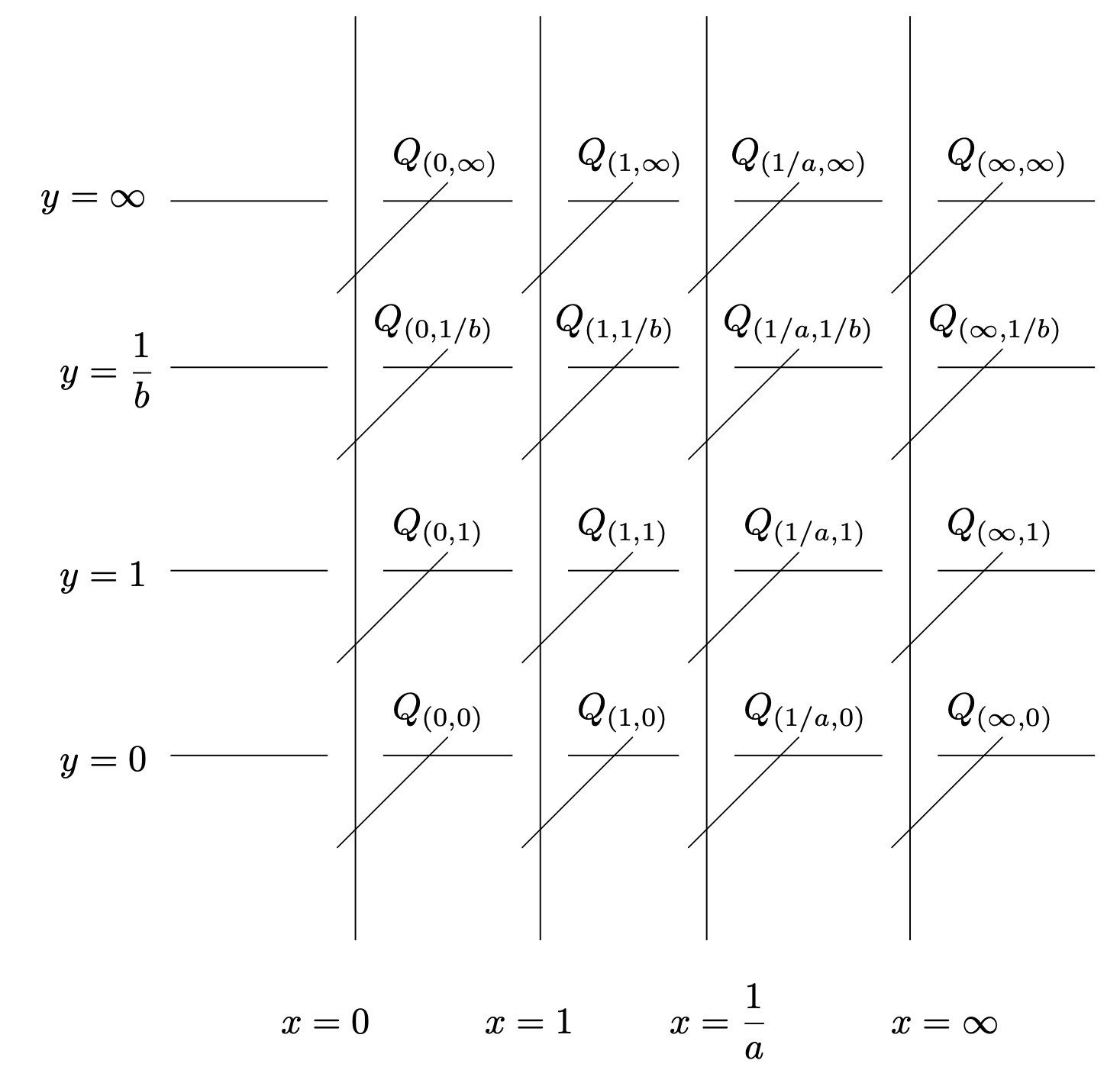
Figure 1. The exceptional divisors $Q_{\sigma}$ on ${\mathcal{X}}$

We constructed the following $T$-schemes.

(47)

We can check that these constructions are all stable under any base change of $T$.

Proposition 3.12.

Let $Z$ be any scheme over $T$. Let ${\mathcal{X}}_{Z},\widetilde{{\mathcal{Y}}}_{Z}$, $(\mathcal{E}\times_{k}\mathcal{E})_{Z}$ and ${\mathcal{Y}}_{Z}$ denote the base changes of ${\mathcal{X}},\widetilde{{\mathcal{Y}}}$, $\mathcal{E}\times_{k}\mathcal{E}$ and ${\mathcal{Y}}$ by $Z\rightarrow T$. Then we have the following.

1. $\widetilde{{\mathcal{Y}}}_{Z}\rightarrow{\mathcal{Y}}_{Z}$ is the double cover associated with $({\mathscr{L}},\eta)$. Here we use the same symbol $({\mathscr{L}},\eta)$ for its pull back by ${\mathcal{Y}}_{Z}\rightarrow{\mathcal{Y}}$.

2. $(\mathcal{E}\times_{k}\mathcal{E})_{Z}\rightarrow\widetilde{{\mathcal{Y}}}_{Z}$ is the quotient by $(\iota\times\iota)_{Z}$. Here $(\iota\times\iota)_{Z}$ is the base change of $\iota\times\iota$.

3. ${\mathcal{X}}_{Z}\rightarrow\widetilde{{\mathcal{Y}}}_{Z}$ is the blowing up along $\Sigma^{2}$.

(3) is not so obvious since the blowing-up is not stable under the base change. But in this case the result follows from the fact that ${\mathcal{O}}_{\widetilde{{\mathcal{Y}}}}/{\mathcal{I}}^{n}$ is flat over $T$ for any $n>0$ where ${\mathcal{I}}$ is the ideal sheaf corresponding to $\Sigma^{2}$.

By the properties of the Legendre family ${\mathcal{E}}\rightarrow S$, we have the following.

Proposition 3.13.

Let $t\in T$ and $O\in\Sigma^{2}$. Then the abelian surface $({\mathcal{E}}\times_{k}{\mathcal{E}})_{t}$ whose identity element is $O$ has the following properties.

1. $\Sigma^{2}$ is the set of 2-torsion points of this abelian surface structure.

2. $(\iota\times\iota)_{t}$ is the involution of taking inverse.

3. Let $a(t),b(t)\in\kappa(t)$ be the images of elements $a,b\in{\mathcal{O}}_{T}(T)$ at the residue field of $t$. Then $({\mathcal{E}}\times_{k}{\mathcal{E}})_{t}$ is isomorphic to the direct product of the elliptic curves $y^{2}=x(1-x)(1-a(t)x)$ and $y^{2}=x(1-x)(1-b(t)x)$ over $\kappa(t)$.

Finally, we prove that ${\mathcal{X}}\rightarrow T$ is a family of Kummer surfaces.

Proposition 3.14.

For $t\in T$, the fiber ${\mathcal{X}}_{t}$ is isomorphic to the Kummer surface associated with the abelian surface $\left(({\mathcal{E}}\times_{k}{\mathcal{E}})_{t},O\right)$ where $O\in\Sigma^{2}$.

Proof.

By Proposition 3.13, $(\iota\times\iota)_{t}$ is the involution of taking inverses on the abelian surface $({\mathcal{E}}\times_{k}{\mathcal{E}})_{t}$. By Proposition 3.12 (2), $({\mathcal{E}}\times_{k}{\mathcal{E}})_{t}\rightarrow\widetilde{{\mathcal{Y}}}_{t}$ corresponds to the quotient by $(\iota\times\iota)_{t}$. Since $\Sigma^{2}\subset({\mathcal{E}}\times_{k}{\mathcal{E}})_{t}(\kappa(t))$ is the set of 2-torsion points on $({\mathcal{E}}\times_{k}{\mathcal{E}})_{t}$, its image $\Sigma^{2}\subset\widetilde{{\mathcal{Y}}}_{t}(\kappa(t))$ corresponds to the set of 16 singular points on $\widetilde{{\mathcal{Y}}}_{t}$. By Proposition 3.12 (3), ${\mathcal{X}}_{t}\rightarrow\widetilde{{\mathcal{Y}}}_{t}$ is the blowing-up of $\widetilde{{\mathcal{Y}}}_{t}$ along these singular points. Hence ${\mathcal{X}}_{t}$ is isomorphic to the Kummer surface associated with $(\mathcal{E}\times_{k}\mathcal{E})_{t}$. ∎

3.3. Construction of other smooth families of varieties over $T$

In this subsection, we define other smooth families of varieties $({\mathcal{E}}\times_{k}{\mathcal{E}}){\widetilde{\phantom{o}}}$ and $\overline{{\mathcal{X}}}$ over $T$ and explain their relations with ${\mathcal{X}}$. These families of varieties are used for relating periods of ${\mathcal{X}}$ with those of elliptic curves in the Legendre family (Section 7) and for a construction of topological 2-chains on fibers ${\mathcal{X}}_{t}$ (Section 8).

Definition 3.15.

Let $({\mathcal{E}}\times_{k}{\mathcal{E}}){\widetilde{\phantom{o}}}$ (resp. $\overline{{\mathcal{X}}}$) be the blowing-up of ${\mathcal{E}}\times_{k}{\mathcal{E}}$ (resp. ${\mathcal{Y}}$) along $\Sigma^{2}$. By the universal property of the blowing-up, we have unique morphisms $({\mathcal{E}}\times_{k}{\mathcal{E}}){\widetilde{\phantom{o}}}\rightarrow{\mathcal{X}}$ and ${\mathcal{X}}\rightarrow\overline{{\mathcal{X}}}$ such that the following diagram commutes.

(48)

The morphism ${\mathcal{X}}\rightarrow\overline{{\mathcal{X}}}$ is described by the following $B$-algebra homomorphisms.

(49)

Finally, we name exceptional divisors on $\overline{{\mathcal{X}}}$. We use this notation in Section 8.

Definition 3.16.

For $\sigma\in\Sigma^{2}$, we define the exceptional divisor $\overline{Q}_{\sigma}\subset\overline{{\mathcal{X}}}$ by the following fiber product.

(50)

The morphism ${\mathcal{X}}\rightarrow\overline{{\mathcal{X}}}$ induces the $2:1$ map $Q_{\sigma}\rightarrow\overline{Q}_{\sigma}$.

4. Construction of automorphisms of the family of Kummer surfaces

As in Section 3, we fix a field $k$ whose characteristic is not 2. Moreover, we assume $k$ contains $\sqrt{-1}$. Until subsection 7.1, we assume these conditions on $k$.

In this section, we will construct a group $\widetilde{G}$ and its action to a scheme ${\mathcal{X}}^{\prime}$, which is a base change of ${\mathcal{X}}$ in Definition 3.10. To construct $\widetilde{G}$-action on ${\mathcal{X}}^{\prime}$, we construct following objects in ${\mathrm{(Sch}^{\mathrm{gp}}/k)}$.

(51)

We will construct them in the following order.

1. We start with $\underline{H}_{0}={\mathrm{Aut}}_{k}(S)=\mathfrak{S}(\{0,1,\infty\})$ (Definition 4.1). We define a $H_{0}\simeq\mathfrak{S}_{4}$-action on ${\mathbb{P}}^{1}_{S}$ so that $\Sigma\subset{\mathrm{Hom}}_{S}(S,{\mathbb{P}}^{1}_{S})$ is compatible with $({\mathbb{P}}^{1}_{S},H_{0})\rightarrow(S,\underline{H}_{0})$. Then we consider their base changes by a finte étale extension ${\mathrm{Spec}\,}A^{\prime}=S^{\prime}\rightarrow S$ (Definition 4.6) and get $(S^{\prime},\underline{H})$ and $({\mathbb{P}}^{1}_{S^{\prime}},H)$. The group $\underline{H}$ is isomorphic to $\mathfrak{S}_{4}$ (Remark 4.8).

2. We define the following objects in ${\mathrm{(Sch}^{\mathrm{gp}}/k)}$ (Definition 4.10)

   $$(T,\underline{G}_{0})=(S\times_{k}S,\underline{H}_{0}\times\underline{H}_{0}), (T^{\prime},\underline{G})=(S^{\prime}\times_{k}S^{\prime},\underline{H}\times\underline{H})$$ (52)

   $$({\mathcal{Y}},G_{0})=({\mathbb{P}}^{1}_{S}\times_{k}{\mathbb{P}}^{1}_{S},H_{0}\times H_{0}), ({\mathcal{Y}}^{\prime},G)=({\mathbb{P}}^{1}_{S^{\prime}}\times_{k}{\mathbb{P}}^{1}_{S^{\prime}},H\times H)$$

3. To lift the $G$-action on ${\mathcal{Y}}^{\prime}$ by the double covering $\widetilde{{\mathcal{Y}}}^{\prime}=\widetilde{{\mathcal{Y}}}\times_{T}T^{\prime}\rightarrow{\mathcal{Y}}^{\prime}$, we use Proposition 2.11. Since $\widetilde{{\mathcal{Y}}}$ is constructed from $({\mathscr{L}},\eta)$ in Definition 3.6, we will construct linearization on ${\mathscr{L}}$ satisfying the liftability condition (33). For this purpose, we consider a group $\widetilde{G}$ which is a ${\mathbb{Z}}/2{\mathbb{Z}}$-extension of $G$ (Definition 4.17).

4. Since the $\widetilde{G}$-action on $\widetilde{{\mathcal{Y}}}^{\prime}$ stabilizes the blowing-up locus of ${\mathcal{X}}^{\prime}\rightarrow\widetilde{{\mathcal{Y}}}^{\prime}$, we can lift $\widetilde{G}$-action on $\widetilde{{\mathcal{Y}}}^{\prime}$ to ${\mathcal{X}}^{\prime}={\mathcal{X}}\times_{T}T^{\prime}$ (Proposition 4.20).

We calculate some opposite 1-cocycles in Subsection 4.4. They are important for the description of the group action on the higher Chow subgroup $\Xi^{\mathrm{can}}$ (Section 6), on the 2-form $\omega\in\Gamma(X,\Omega_{{\mathcal{X}}^{\prime}/T^{\prime}}^{2})$ (Section 7) and on the sheaf ${\mathcal{Q}}_{\omega}$ (Section 9).

4.1. Automorphisms on $S$ and ${\mathbb{P}}^{1}_{S}$

In this subsection, we construct objects and a morphism $({\mathbb{P}}^{1}_{S},H_{0})\rightarrow(S,\underline{H}_{0})$ in ${\mathrm{(Sch}^{\mathrm{gp}}/k)}$.

Definition 4.1.

We define $\underline{H}_{0}={\mathrm{Aut}}_{k}(S)$. If we regard $S={\mathbb{P}}^{1}_{k}-\{0,1,\infty\}$, every $\underline{\tau}_{0}\in\underline{H}_{0}$ extends to an automorphism on ${\mathbb{P}}^{1}_{k}$ which stabilizes the $k$-rational point set $\{0,1,\infty\}$. Hence we have the following group isomorphism.

(53)

We often identify $\underline{H}_{0}$ with $\mathfrak{S}(\{0,1,\infty\})$. The correspondence of $\underline{H}_{0}$ and $\mathfrak{S}(\{0,1,\infty\})$ is given in Table 1. Note that the composition on $\mathfrak{S}(\{0,1,\infty\})$ is defined as the usual order. For example, $(0\>1)(0\>\infty)=(0\>\infty\>1)$. Thus $\underline{H}_{0}$ induces an opposite action on the ring $A$.

Table 1. The correspondence of $\underline{H}_{0}\simeq\mathfrak{S}(\{0,1,\infty\})$

$\underline{\tau}_{0}$	$\underline{\tau}_{0}^{\sharp}(c)$	$\underline{\tau}_{0}$	$\underline{\tau}_{0}^{\sharp}(c)$
${\mathrm{id}}$	$c$	$(0\;1)$	$1-c$
$(1\;\infty)$	$\frac{c}{c-1}$	$(0\;1\;\infty)$	$\frac{1}{1-c}$
$(0\;\infty)$	$\frac{1}{c}$	$(0\;\infty\;1)$	$\frac{c-1}{c}$

Next, we define a subgroup $H_{0}$ of the automorphism group of ${\mathbb{P}}^{1}_{S}$. Using the notation in Definition 2.1, we have the following group.

$${\mathrm{Aut}}({\mathbb{P}}^{1}_{S};S,\underline{H}_{0})=\left\{(\tau_{0},\underline{\tau}_{0})\in{\mathrm{Aut}}_{k}({\mathbb{P}}^{1}_{S})\times\underline{H}_{0}:\leavevmode\hbox to61.38pt{\vbox to53.84pt{\text{[drawing]}}}\quad\text{commutes.}\right\} {{\mathbb{P}}^{1}_{S}} {S} {{\mathbb{P}}^{1}_{S}} {S} \scriptstyle{\tau_{0}} \scriptstyle{\underline{\tau}_{0}} {{\mathbb{P}}^{1}_{S}} {S} {{\mathbb{P}}^{1}_{S}} {S} \scriptstyle{\tau_{0}} \scriptstyle{\underline{\tau}_{0}}$$ (54)

Since the natural projection ${\mathrm{Aut}}({\mathbb{P}}^{1}_{S};S,\underline{H}_{0})\rightarrow{\mathrm{Aut}}_{k}({\mathbb{P}}^{1}_{S})$ is injective, we identify ${\mathrm{Aut}}({\mathbb{P}}^{1}_{S};S,\underline{H}_{0})$ as a subgroup of ${\mathrm{Aut}}_{k}({\mathbb{P}}^{1}_{S})$. We often denote an element in ${\mathrm{Aut}}({\mathbb{P}}^{1}_{S};S,\underline{H}_{0})$ by $\tau_{0}$. For $\tau_{0}\in{\mathrm{Aut}}({\mathbb{P}}^{1}_{S};S,\underline{H}_{0})$, the image of $\tau_{0}$ under the natural projection ${\mathrm{Aut}}({\mathbb{P}}^{1}_{S};S,\underline{H}_{0})\rightarrow\underline{H}_{0}$ is denoted by $\underline{\tau}_{0}$.

Definition 4.2.

We define $H_{0}$ as the following subgroup of ${\mathrm{Aut}}({\mathbb{P}}^{1}_{S};S,\underline{H}_{0})$.

$$H_{0}=\left\{\tau_{0}\in{\mathrm{Aut}}({\mathbb{P}}^{1}_{S};S,\underline{H}_{0}):\text{For any }\sigma\in\Sigma\text{, }\tau_{0}\circ\sigma\circ\underline{\tau}_{0}^{-1}\in\Sigma.\right\}$$ (55)

Then we have a natural morphism $\alpha:({\mathbb{P}}^{1}_{S},H_{0})\rightarrow(S,\underline{H}_{0})$ in ${\mathrm{(Sch}^{\mathrm{gp}}/k)}$. By the construction, $\Sigma$ is compatible with $\alpha:({\mathbb{P}}^{1}_{S},H_{0})\rightarrow(S,\underline{H}_{0})$. By Definition 2.3, $H_{0}$ has the following natural set-theoretic action on $\Sigma$.

(56)

Proposition 4.3.

The group homomorphism $(\ref{grouphom})$ is an isomorphism.

Proof.

Let $\tau_{0}\in H_{0}$. We have the following diagram.

(57)

where $\underline{\tau}_{0}^{-1}:{\mathbb{P}}^{1}_{S}\rightarrow{\mathbb{P}}^{1}_{S}$ is the morphism ${\mathrm{id}}_{{\mathbb{P}}^{1}_{k}}\times\underline{\tau}_{0}^{-1}:{\mathbb{P}}^{1}_{S}={\mathbb{P}}^{1}_{k}\times_{k}S\rightarrow{\mathbb{P}}^{1}_{k}\times_{k}S={\mathbb{P}}^{1}_{S}$. Then $(\underline{\tau}_{0}^{-1})^{\sharp}(z)=z$ where $z$ is the inhomogeneous coordinate on ${\mathbb{P}}^{1}_{S}$ in Definition 3.1. Since $\underline{\tau}_{0}^{-1}\circ\tau_{0}:{\mathbb{P}}^{1}_{S}\rightarrow{\mathbb{P}}^{1}_{S}$ is a morphism over $S$, we can write $(\underline{\tau}_{0}^{-1}\circ\tau_{0})^{\sharp}(z)=\frac{pz+q}{rz+s}$ where $p,q,r,s\in A$. Hence we can write

$$\tau_{0}^{\sharp}(z)=\frac{pz+q}{rz+s}\quad(p,q,r,s\in A).$$ (58)

First, we check (56) is injective. Suppose $\tau_{0}\in H_{0}$ lies in the kernel of (56). Since $\tau_{0}$ acts trivially on $\Sigma$, $\tau_{0}(0)=0$, $\tau_{0}(1)=1$, $\tau_{0}(1/c)=1/c$ and $\tau_{0}(\infty)=\infty$. Especially we have

$$\frac{p\cdot 0+q}{r\cdot 0+s}=0,\quad \frac{p\cdot 1+q}{r\cdot 1+s}=1,$$ (59)

$$\frac{p\cdot\frac{1}{c}+q}{r\cdot\frac{1}{c}+s}=\frac{1}{\underline{\tau}_{0}^{\sharp}(c)},\quad \frac{p\cdot\infty+q}{r\cdot\infty+s}=\infty.$$

Hence we see that $\tau_{0}^{\sharp}(z)=z$ and $\underline{\tau}_{0}^{\sharp}(c)=c$. i.e. $\tau_{0}={\mathrm{id}}_{H_{0}}$.

Next, we check that (56) is surjective. It is enough to find elements in $H_{0}$ corresponding to $(0\>1),(0\>1\>1/c\>\infty)\in\mathfrak{S}(\Sigma)$ since they are generators of $\mathfrak{S}(\Sigma)$. We use the presentation in (58) again. For example, to find $\tau_{0}\in H_{0}$ corresponding to $(0\>1\>1/c\>\infty)$, it is enough to find $p,q,r,s\in A$ such that

$$\frac{p\cdot 0+q}{r\cdot 0+s}=1,\quad \frac{p\cdot 1+q}{r\cdot 1+s}=\frac{1}{\underline{\tau}_{0}^{\sharp}(c)},$$ (60)

$$\frac{p\cdot\frac{1}{c}+q}{r\cdot\frac{1}{c}+s}=\infty,\quad \frac{p\cdot\infty+q}{r\cdot\infty+s}=0.$$

From these conditions, we can find a pair of automorphisms $(\tau_{0},\underline{\tau}_{0})\in{\mathrm{Aut}}_{k}({\mathbb{P}}^{1}_{S})\times\underline{H}_{0}$ such that $\tau_{0}^{\sharp}(z)=\frac{1}{1-cz}$ and $\underline{\tau}_{0}^{\sharp}(c)=1-c$, which is in $H_{0}$ and its image under the map (56) is $(0\>1\>1/c\>\infty)\in\mathfrak{S}(\Sigma)$. Similarly, we can find the element of $H_{0}$ such that its image under the map (56) is $(0\>1)\in\mathfrak{S}(\Sigma)$. ∎

Remark 4.4.

By Proposition 4.3, we often identify $H_{0}$ with $\mathfrak{S}(\Sigma)$. The explicit correspondence of $H_{0}\simeq\mathfrak{S}(\Sigma)$ is given in Table 2. We can find these correspondence by the same method we use in the proof of Proposition 4.3. In the table, for each $\tau_{0}\in H_{0}$, the image of $c$ under $\underline{\tau}_{0}^{\sharp}:A\rightarrow A$ and the image of the local coordinate $z$ under $\tau_{0}^{\sharp}:{\mathcal{O}}_{{\mathbb{P}}^{1}_{S}}\rightarrow(\tau_{0})_{*}{\mathcal{O}}_{{\mathbb{P}}^{1}_{S}}$ are given.

Table 2. The correspondence of $H_{0}\simeq\mathfrak{S}(\{0,1,1/c,\infty\})$

$\tau_{0}$	$\underline{\tau}_{0}^{\sharp}(c)$	$\tau_{0}^{\sharp}(z)$
${\mathrm{id}}$	$c$	$z$

$\tau_{0}$	$\underline{\tau}_{0}^{\sharp}(c)$	$\tau_{0}^{\sharp}(z)$	$\tau_{0}$	$\underline{\tau}_{0}^{\sharp}(c)$	$\tau_{0}^{\sharp}(z)$	$\tau_{0}$	$\underline{\tau}_{0}^{\sharp}(c)$	$\tau_{0}^{\sharp}(z)$
$(0\;1)$	$\frac{c}{c-1}$	$1-z$	$(0\;1/c)$	$1-c$	$\frac{1-cz}{1-c}$	$(0\;\infty)$	$\frac{1}{c}$	$\frac{1}{z}$
$(1/c\;\infty)$	$\frac{c}{c-1}$	$\frac{(1-c)z}{1-cz}$	$(1\;\infty)$	$1-c$	$\frac{z}{z-1}$	$(1\;1/c)$	$\frac{1}{c}$	$cz$

$\tau_{0}$	$\underline{\tau}_{0}^{\sharp}(c)$	$\tau_{0}^{\sharp}(z)$	$\tau_{0}$	$\underline{\tau}_{0}^{\sharp}(c)$	$\tau_{0}^{\sharp}(z)$	$\tau_{0}$	$\underline{\tau}_{0}^{\sharp}(c)$	$\tau_{0}^{\sharp}(z)$
$(0\;1)(1/c\;\infty)$	$c$	$\frac{1-z}{1-cz}$	$(0\;1/c)(1\;\infty)$	$c$	$\frac{1-cz}{c(1-z)}$	$(0\;\infty)(1\;1/c)$	$c$	$\frac{1}{cz}$

$\tau_{0}$	$\underline{\tau}_{0}^{\sharp}(c)$	$\tau_{0}^{\sharp}(z)$	$\tau_{0}$	$\underline{\tau}_{0}^{\sharp}(c)$	$\tau_{0}^{\sharp}(z)$
$(0\;1\;1/c)$	$\frac{1}{1-c}$	$1-cz$	$(0\;1/c\;1)$	$\frac{c-1}{c}$	$\frac{c(1-z)}{c-1}$
$(0\;\infty\;1)$	$\frac{1}{1-c}$	$\frac{z-1}{z}$	$(0\;1\;\infty)$	$\frac{c-1}{c}$	$\frac{1}{1-z}$
$(0\;1/c\;\infty)$	$\frac{1}{1-c}$	$\frac{1-c}{1-cz}$	$(0\;\infty\;1/c)$	$\frac{c}{c-1}$	$\frac{1-cz}{(1-c)z}$
$(1\;\infty\;1/c)$	$\frac{1}{1-c}$	$\frac{(c-1)z}{1-z)}$	$(1\;1/c\;\infty)$	$\frac{c-1}{c}$	$\frac{cz}{cz-1}$

$\tau_{0}$	$\underline{\tau}_{0}^{\sharp}(c)$	$\tau_{0}^{\sharp}(z)$	$\tau_{0}$	$\underline{\tau}_{0}^{\sharp}(c)$	$\tau_{0}^{\sharp}(z)$	$\tau_{0}$	$\underline{\tau}_{0}^{\sharp}(c)$	$\tau_{0}^{\sharp}(z)$
$(0\;1/c\;1\;\infty)$	$\frac{c}{c-1}$	$\frac{c-1}{c(1-z)}$	$(0\;1\;1/c\;\infty)$	$1-c$	$\frac{1}{1-cz}$	$(0\;1\;\infty\;1/c)$	$\frac{1}{c}$	$\frac{1-cz}{1-z}$
$(0\;\infty\;1\;1/c)$	$\frac{c}{c-1}$	$\frac{cz-1}{cz}$	$(0\;\infty\;1/c\;1)$	$1-c$	$\frac{1-z}{(c-1)z}$	$(0\;1/c\;\infty\;1)$	$\frac{1}{c}$	$\frac{c(1-z)}{1-cz}$

Remark 4.5.

We have a bijection

$$\{\{\{0,1\},\{\infty,1/c\}\},\{\{0,\infty\},\{1,1/c\}\},\{\{0,1/c\},\{1,\infty\}\}\}\simeq\{0,1,\infty\}$$ (61)

defined by $\{\{0,1\},\{\infty,1/c\}\}\mapsto 0,\{\{0,\infty\},\{1,1/c\}\}\mapsto 1,\{\{0,1/c\},\{1,\infty\}\}\}\mapsto\infty$. Since $\mathfrak{S}(\Sigma)$ acts on the set on the left hand side, we have a group homomorphism

$$\mathfrak{S}(\Sigma)\>{\longrightarrow}\>\mathfrak{S}(\{0,1,\infty\})$$ (62)

The group homomorphism $H_{0}\rightarrow\underline{H}_{0}$ is identified with the group homomorphism (62) under the identifications $H_{0}=\mathfrak{S}(\Sigma)$ and $\underline{H}_{0}=\mathfrak{S}(\{0,1,\infty\})$.

4.2. A finite étale covering $S^{\prime}\rightarrow S$ and lifts of group actions

To get enough automorphisms of the family of Kummer surfaces, we have to enlarge the base scheme $S$. As we will see later in Section 5, this base change is also necessary for the construction of higher Chow cycles in $\Xi^{\mathrm{can}}$.

Definition 4.6.

We define an $A$-algebra $A^{\prime}$ as $A^{\prime}=A[\sqrt{c},\sqrt{1-c}]$ and $S^{\prime}={\mathrm{Spec}\,}A^{\prime}$. We have a natural morphism $S^{\prime}\rightarrow S$ induced by $A\hookrightarrow A^{\prime}$. Furthermore, we define $\underline{H}={\mathrm{Aut}}(S^{\prime};S,\underline{H}_{0})$. i.e.

$$\underline{H}=\left\{(\underline{\tau},\underline{\tau}_{0})\in{\mathrm{Aut}}_{k}(S^{\prime})\times\underline{H}_{0}:\leavevmode\hbox to60.02pt{\vbox to49.52pt{\text{[drawing]}}}\quad\text{commutes.}\right\} {S^{\prime}} {S} {S^{\prime}} {S} \scriptstyle{\underline{\tau}} \scriptstyle{\underline{\tau}_{0}} {S^{\prime}} {S} {S^{\prime}} {S} \scriptstyle{\underline{\tau}} \scriptstyle{\underline{\tau}_{0}}$$ (63)

Then we have a natural morphism $\beta:(S^{\prime},\underline{H})\rightarrow(S,\underline{H}_{0})$ in ${\mathrm{(Sch}^{\mathrm{gp}}/k)}$. Since the natural projection $\underline{H}\rightarrow{\mathrm{Aut}}_{k}(S^{\prime})$ is injective, we regard $\underline{H}$ as a subgroup of ${\mathrm{Aut}}_{k}(S^{\prime})$. We often denote an element in $\underline{H}$ by $\underline{\tau}$. For $\underline{\tau}\in\underline{H}$, the image of $\underline{\tau}$ under the natural projection $\underline{H}\rightarrow\underline{H}_{0}$ is denoted by $\underline{\tau}_{0}\in\underline{H}_{0}$.

Proposition 4.7.

We have the following properties about $(S^{\prime},\underline{H})$.

1. $S^{\prime}\rightarrow S$ is a finite étale morphism.

2. We have the following isomorphism between $k$-algebras. Especially, $A^{\prime}$ is an integral domain.

   (64)

3. The group homomorphism $\underline{H}\rightarrow\underline{H}_{0}$ is surjective.

4. The kernel of $\underline{H}\rightarrow\underline{H}_{0}$ is isomorphic to $\mu_{2}(k)\times\mu_{2}(k)$.

Especially, $\underline{H}$ fits into the following exact sequence.

$$1\>{\longrightarrow}\>\mu_{2}(k)\times\mu_{2}(k)\>{\longrightarrow}\>\underline{H}\>{\longrightarrow}\>\underline{H}_{0}\>{\longrightarrow}\>1$$ (65)

Proof.

We can show (1), (2) and (4) by the ring theoretic calculation. To prove (3), we construct the lifts of $\underline{\tau}_{0}\in\underline{H}_{0}$ explicitly. The result is summarized in Table 3. In the table, we give the image of $\gamma\in k\left[\gamma,\frac{1}{\gamma(\gamma^{4}-1)}\right]$ under the ring homomorphisms $\underline{\tau}^{\sharp}:k\left[\gamma,\frac{1}{\gamma(\gamma^{4}-1)}\right]\simeq A^{\prime}\rightarrow A^{\prime}\simeq k\left[\gamma,\frac{1}{\gamma(\gamma^{4}-1)}\right]$ corresponding to the lifts of each $\underline{\tau}_{0}^{\sharp}:A\rightarrow A$. ∎

Table 3. The lifts of $\tau_{0}\in\underline{H}_{0}$ to $\underline{H}$

$\underline{\tau}_{0}^{\sharp}(c)$	$\underline{\tau}^{\sharp}(\gamma)$	$\underline{\tau}_{0}^{\sharp}(c)$	$\underline{\tau}^{\sharp}(\gamma)$
$c$	$\pm\gamma,\pm\frac{1}{\gamma}$	$1-c$	$\pm\sqrt{-1}\gamma,\pm\sqrt{-1}\frac{1}{\gamma}$
$\frac{c}{c-1}$	$\pm\frac{\gamma+1}{\gamma-1},\pm\frac{\gamma-1}{\gamma+1}$	$\frac{1}{1-c}$	$\pm\sqrt{-1}\frac{\gamma+1}{\gamma-1},\pm\sqrt{-1}\frac{\gamma-1}{\gamma+1}$
$\frac{c-1}{c}$	$\pm\frac{\gamma+\sqrt{-1}}{\gamma-\sqrt{-1}},\pm\frac{\gamma-\sqrt{-1}}{\gamma+\sqrt{-1}}$	$\frac{1}{c}$	$\pm\sqrt{-1}\frac{\gamma+\sqrt{-1}}{\gamma-\sqrt{-1}},\pm\sqrt{-1}\frac{\gamma-\sqrt{-1}}{\gamma+\sqrt{-1}}$

Remark 4.8.

More strongly, we can show that $\underline{H}$ is isomorphic to $\mathfrak{S}_{4}$ as follows. By the isomorphism (64) in Proposition 4.7, we can regard $S^{\prime}={\mathbb{P}}^{1}_{k}-\{\pm 1,\pm\sqrt{-1},0,\infty\}$. Let $N=\{\pm 1,\pm\sqrt{-1},0,\infty\}\subset{\mathbb{P}}^{1}_{k}(k)$. If we plot points of $N$ on the Riemann sphere ${\mathbb{P}}^{1}({\mathbb{C}})$, $N$ forms an octahedron. We can check that $\underline{H}$ acts on this octahedron and $\underline{H}$ is naturally isomorphic to the octahedral group, which is isomorphic to $\mathfrak{S}_{4}$.

Definition 4.9.

We define $({\mathbb{P}}^{1}_{S^{\prime}},H)\in{\mathrm{(Sch}^{\mathrm{gp}}/k)}$ as a fiber product of $({\mathbb{P}}^{1}_{S},H_{0})$ and $(S^{\prime},\underline{H})$ over $(S,\underline{H}_{0})$ in ${\mathrm{(Sch}^{\mathrm{gp}}/k)}$.

(66)

By Proposition 2.2, $H$ is equal to the fiber product

$$H_{0}\times_{\underline{H}_{0}}\underline{H}=\left\{\tau=(\tau_{0},\underline{\tau})\in H_{0}\times\underline{H}:\alpha(\tau_{0})=\beta(\underline{\tau})\right\}$$ (67)

where $\alpha$ and $\beta$ are group homomorphisms corresponding to $\alpha:({\mathbb{P}}^{1}_{S},H_{0})\rightarrow(S,\underline{H}_{0})$ and $\beta:(S^{\prime},\underline{H})\rightarrow(S,\underline{H}_{0})$. Since $H_{0}\simeq\underline{H}\simeq\mathfrak{S}_{4}$ (Proposition 4.3 and Remark 4.8) and $\underline{H}_{0}\simeq\mathfrak{S}_{3}$ (Definition 4.1), we have $H\simeq\mathfrak{S}_{4}\times_{\mathfrak{S}_{3}}\mathfrak{S}_{4}$.

By definition, we have the following natural group homomorphisms $H\rightarrow\underline{H}$ and $H\rightarrow H_{0}$. By Remark 4.5 and Proposition 4.7, they are surjective.

(68)

The images of $\tau\in H$ in $H_{0}$ and $\underline{H}$ are denoted by $\tau_{0}\in H_{0}$ and $\underline{\tau}\in\underline{H}$, respectively.

Definition 4.10.

We define the following objects in ${\mathrm{(Sch}^{\mathrm{gp}}/k)}$.

$$(T,\underline{G}_{0})=(S,\underline{H}_{0})\times(S,\underline{H}_{0}), ({\mathcal{Y}},G_{0})=({\mathbb{P}}^{1}_{S},H_{0})\times({\mathbb{P}}^{1}_{S},H_{0})$$ (69)

$$(T^{\prime},\underline{G})=(S^{\prime},\underline{H})\times(S^{\prime},\underline{H}), ({\mathcal{Y}}^{\prime},G)=({\mathbb{P}}^{1}_{S^{\prime}},H)\times({\mathbb{P}}^{1}_{S^{\prime}},H)$$

By Proposition 2.2, $\underline{G}_{0},G_{0},\underline{G}$ and $G$ coincide with $\underline{H}_{0}\times\underline{H}_{0},H_{0}\times H_{0},\underline{H}\times\underline{H}$ and $H\times H$. By considering the direct products of morphisms in (66), we have the following morphisms in ${\mathrm{(Sch}^{\mathrm{gp}}/k)}$.

(70)

By checking the universality, we see that the left diagram in (70) is the fiber product. Especially, ${\mathcal{Y}}^{\prime}$ is the base change of ${\mathcal{Y}}$ by $T^{\prime}\rightarrow T$. We denote the images of $\rho\in G$ under the group homomorphisms in (70) by $\underline{\rho}\in\underline{G}$, $\rho_{0}\in G_{0}$ and $\underline{\rho}_{0}\in\underline{G}_{0}$ respectively. Furthermore, for $\rho\in G$, its first and second components are denoted by $\rho^{(1)}$ and $\rho^{(2)}$ respectively. i.e.

$$G=\{\rho=(\rho^{(1)},\rho^{(2)}):\rho^{(1)},\rho^{(2)}\in H\}$$ (71)

We define $\underline{\rho}_{0}^{(i)},\rho_{0}^{(i)},\underline{\rho}^{(i)}$ for $i=1,2$ similarly.

Definition 4.11.

We define $B^{\prime}=A^{\prime}\otimes_{k}A^{\prime}$. By definition, $T^{\prime}={\mathrm{Spec}\,}B^{\prime}$. For any scheme $Z$ over $T$, $Z^{\prime}$ denotes the base change of $Z$ by $T^{\prime}\rightarrow T$. For example, $\widetilde{{\mathcal{Y}}}^{\prime}=\widetilde{{\mathcal{Y}}}\times_{T}T^{\prime}$, ${\mathcal{X}}^{\prime}={\mathcal{X}}\times_{T}T^{\prime}$ and $Q^{\prime}_{\sigma}=Q_{\sigma}\times_{T}T^{\prime}$. This notation is compatible with ${\mathcal{Y}}^{\prime}={\mathcal{Y}}\times_{T}T^{\prime}$.

Proposition 4.12.

The $B^{\prime}$-rational point set $\Sigma^{2}({\mathcal{Y}}^{\prime})$ is compatible with $({\mathcal{Y}}^{\prime},G)\rightarrow(T^{\prime},\underline{G})$. Especially, $G$ has a natural action on $\Sigma^{2}$.

Proof.

By Definition 4.2, $\Sigma({\mathbb{P}}^{1}_{S})$ is compatible with $({\mathbb{P}}^{1}_{S},H_{0})\rightarrow(S,\underline{H}_{0})$. Then by Proposition 2.4, $\Sigma({\mathbb{P}}^{1}_{S^{\prime}})$ is compatible with $({\mathbb{P}}^{1}_{S^{\prime}},H)\rightarrow(S^{\prime},\underline{H})$. Since $({\mathcal{Y}}^{\prime},G)\rightarrow(T^{\prime},\underline{G})$ is the direct product of $({\mathbb{P}}^{1}_{S^{\prime}},H)\rightarrow(S^{\prime},\underline{H})$, $\Sigma^{2}({\mathcal{Y}}^{\prime})$ is compatible with $({\mathcal{Y}}^{\prime},G)\rightarrow(T^{\prime},\underline{G})$ by Proposition 2.4 again. ∎

4.3. Linearizations on ${\mathscr{L}}$ and cocycles $\phi,\chi$

In this subsection, we define a linearization of ${\mathscr{L}}$ which give rise to a lifting of the $G$-action on ${\mathcal{Y}}^{\prime}$ to $\widetilde{{\mathcal{Y}}}^{\prime}$. Since ${\mathscr{L}}=pr_{1}^{*}\Omega^{1}_{{\mathbb{P}}^{1}_{S^{\prime}}/S^{\prime}}\otimes_{{\mathcal{O}}_{{\mathcal{Y}}^{\prime}}}pr_{2}^{*}\Omega^{1}_{{\mathbb{P}}^{1}_{S^{\prime}}/S^{\prime}}$, we have a $G$-linearization $\{\Psi_{\rho}\}_{\rho\in G}$ on ${\mathscr{L}}$. However, by this natural $G$-linearization, $\Psi_{\rho}^{\otimes(-2)}(\rho^{*}(\eta))$ and $\eta$ differs by

$$\Psi_{\rho}^{\otimes(-2)}(\rho^{*}(\eta))=\chi_{0}(\rho)^{-1}\cdot\eta.$$ (72)

where $\chi_{0}$ is an opposite 1-cocycle. The first aim of this subsection is to get the explicit description of this $\chi_{0}$. Then we will find an opposite 1-cocycle $\widetilde{\chi}$ such that $\widetilde{\chi}^{2}=\chi_{0}$. For this purpose, we introduce opposite coboundary 1-cocycles $\chi$, $\chi^{(1)}$ and $\chi^{(2)}$ and take a ${\mathbb{Z}}/2{\mathbb{Z}}$-extension $\widetilde{G}$ of $G$. Finally, using $\widetilde{\chi}$, we modify the linearization $\{\Psi_{\rho}\}_{\rho\in G}$ on ${\mathscr{L}}$ and get a new $\widetilde{G}$-linearization $\{X_{\widetilde{\rho}}\}_{\widetilde{\rho}\in\widetilde{G}}$ on ${\mathscr{L}}$ which satisfies the liftability condition (33) in Proposition 2.11.

Definition-Proposition 4.13.

We define $H$-linearization $\{\Phi_{\tau}\}_{\tau\in H}$ of $\Omega^{1}_{{\mathbb{P}}^{1}_{S^{\prime}}/S^{\prime}}$ as the canonical one induced by Proposition 2.6. By definition, $\{\Phi_{\tau}\}_{\tau\in H}$ satisfies

$$\Phi_{\tau}\left(\tau^{*}(dz)\right)=\frac{\partial}{\partial z}(\tau^{\sharp}(z))\cdot dz.$$ (73)

We define an opposite 1-cocycle $\phi_{0}:H\rightarrow R({\mathbb{P}}^{1}_{S^{\prime}})^{\times}$ as the opposite 1-cocycle associated with $\left((\Omega^{1}_{{\mathbb{P}}^{1}_{S^{\prime}}/S^{\prime}})^{\otimes(-2)},\{\Phi_{\tau}^{\otimes(-2)}\}_{\tau\in H},\widetilde{h}\right)$, where $\widetilde{h}$ is the section defined in Definition 3.1. By definition, $\phi_{0}(\tau)$ can be computed as follows.

$$\phi_{0}(\tau)=\left(\frac{\partial}{\partial z}(\tau^{\sharp}(z))\right)^{2}\frac{h(z)}{\tau^{\sharp}(h(z))}$$ (74)

By the computation of $\phi_{0}(\tau)$ for each $\tau\in H$, we have the following properties.

1. $\phi_{0}(\tau)$ is determined by the image of $\tau$ under $H\rightarrow\underline{H}_{0}$.

2. The explicit description of $\phi_{0}(\tau)$ is given by the following table.

   Table 4. The opposite 1-cocycle $\phi_{0}$

   $\underline{\tau}_{0}$	$\underline{\tau}_{0}^{\sharp}(c)$	$\phi_{0}(\underline{\tau}_{0})$	$\underline{\tau}_{0}$	$\underline{\tau}_{0}^{\sharp}(c)$	$\phi_{0}(\underline{\tau}_{0})$
   ${\mathrm{id}}$	$c$	$1$	$(0\>1)$	$1-c$	$-1$
   $(1\>\infty)$	$\frac{c}{c-1}$	$1-c$	$(0\>1\>\infty)$	$\frac{1}{1-c}$	$c-1$
   $(0\>\infty)$	$\frac{1}{c}$	$c$	$(0\>\infty\>1)$	$\frac{c-1}{c}$	$-c$

   Especially, $\phi_{0}(\tau)\in A^{\times}$.

From these properties, we regard $\phi_{0}$ as the opposite 1-cocycle $\underline{H}_{0}\rightarrow A^{\times}$.

Definition 4.14.

(Definition of $\chi_{0}$) For $i=1,2$, we have an $G$-linearization $\{pr_{i}^{*}\Phi_{\rho^{(i)}}\}_{\rho\in G}$ of $pr_{i}^{*}\Omega^{1}_{{\mathbb{P}}^{1}_{S^{\prime}}/S^{\prime}}$ by pulling back (cf. Proposition 2.7) the $H$-linearization of $\Omega^{1}_{{\mathbb{P}}^{1}_{S^{\prime}}/S^{\prime}}$ in Definition 4.13 by $pr_{i}:{\mathcal{Y}}^{\prime}\rightarrow{\mathbb{P}}^{1}_{S^{\prime}}$. Then we define a $G$-linearization $\{\Psi_{\rho}\}_{\rho\in G}$ of ${\mathscr{L}}=pr_{1}^{*}\Omega^{1}_{{\mathbb{P}}^{1}_{S^{\prime}}/S^{\prime}}\otimes_{{\mathcal{O}}_{{\mathcal{Y}}^{\prime}}}pr_{2}^{*}\Omega^{1}_{{\mathbb{P}}^{1}_{S^{\prime}}/S^{\prime}}$ by

$$\Psi_{\rho}=pr_{1}^{*}\Phi_{\rho^{(1)}}\otimes pr_{2}^{*}\Phi_{\rho^{(2)}}.$$ (75)

Since $pr_{1}^{\sharp}(h(z))=f(x)$ and $pr_{2}^{\sharp}(h(z))=g(y)$, we have

$$pr_{1}^{\sharp}(\phi_{0}(\rho^{(1)}))=\left(\frac{\partial}{\partial x}(\rho^{\sharp}(x))\right)^{2}\frac{f(x)}{\rho^{\sharp}(f(x))}$$ (76)

$$pr_{2}^{\sharp}(\phi_{0}(\rho^{(2)}))=\left(\frac{\partial}{\partial y}(\rho^{\sharp}(y))\right)^{2}\frac{g(y)}{\rho^{\sharp}(g(y))}.$$

We define $\chi_{0}$ as the opposite 1-cocycle associated with $({\mathscr{L}},\{\Psi_{\rho}^{\otimes(-2)}\}_{\rho\in G},\eta)$. By definition, we have the following equations.

$$\Psi_{\rho}^{\otimes(-2)}(\rho^{*}(\eta))=\chi_{0}(\rho)^{-1}\cdot\eta$$ (77)

$$\chi_{0}(\rho)=pr_{1}^{\sharp}(\phi_{0}(\rho^{(1)}))pr_{2}^{\sharp}(\phi_{0}(\rho^{(2)}))\in B^{\times}$$ (78)

By (78), we can calculate $\chi_{0}$ from Table 4.

We will find an opposite 1-cocycle $\widetilde{\chi}$ such that $\widetilde{\chi}^{2}=\chi_{0}$. First, we will find an opposite coboundary 1-cocycle $\phi$ of $\underline{H}$ whose square coincides with $\phi_{0}$ up to sign.

Definition-Proposition 4.15.

$($Definition of $\phi$$)$ For $\tau\in\underline{H}$, we define

$$\phi(\underline{\tau})=\underline{\tau}^{\sharp}\left(\frac{\sqrt{c}\sqrt{1-c}}{c^{2}-c+1}\right)\cdot\left(\frac{\sqrt{c}\sqrt{1-c}}{c^{2}-c+1}\right)^{-1}.$$ (79)

The explicit description of $\phi$ is given in Table 6 in Section 9. The opposite 1-cocycle $\phi$ of $\underline{H}$ has the following properties.

1. For $\tau\in H$, we have

   $$\phi_{0}(\tau)={\mathrm{sgn}}(\underline{\tau}_{0})\cdot\phi(\underline{\tau})^{2}.$$ (80)

   where ${\mathrm{sgn}}:\underline{H}_{0}\simeq\mathfrak{S}(\{0,1,\infty\})\rightarrow\{\pm 1\}$ is the sign map.

2. For $\underline{\tau}\in\underline{H}$, $\phi(\underline{\tau})\in(A^{\prime})^{\times}$.

Proof.

To prove (1), it is enough to calculate

$$\phi(\underline{\tau})^{2}=\underline{\tau}^{\sharp}\left(\frac{c(1-c)}{(c^{2}-c+1)^{2}}\right)\cdot\left(\frac{c(1-c)}{(c^{2}-c+1)^{2}}\right)^{-1}$$ (81)

Since the right hand side of the above equation depends only on the image $\underline{\tau}_{0}\in\underline{H}_{0}$ of $\underline{\tau}\in\underline{H}$ under $\underline{H}\rightarrow\underline{H}_{0}$ and $\phi_{0}(\tau)$ also depends only on $\underline{\tau}_{0}$ by Proposition 4.13, it is enough to check (80) for each $\underline{\tau}_{0}\in\underline{H}_{0}$ by using Table 1 and Table 4. (2) follows from (1). ∎

We get an opposite 1-cocycle $\chi$ of $\underline{G}$ whose square coincides with $\chi_{0}$ up to sign.

Definition 4.16.

(Definition of $\chi^{(1)},\chi^{(2)}$ and $\chi$) For $\underline{\rho}\in\underline{G}$, we define

$$\chi^{(i)}(\underline{\rho})=pr_{i}^{\sharp}(\phi(\underline{\rho}^{(i)})) \in(B^{\prime})^{\times}\quad\text{for }i=1,2$$ (82)

$$\chi(\underline{\rho})=\chi^{(1)}(\underline{\rho})\cdot\chi^{(2)}(\underline{\rho}) \in(B^{\prime})^{\times}.$$

By Proposition 4.15, $\chi$ satisfies the following equation for $\rho\in G$.

$$\chi_{0}(\rho)={\mathrm{sgn}}(\underline{\rho}_{0}^{(1)}){\mathrm{sgn}}(\underline{\rho}_{0}^{(2)})\cdot\chi(\underline{\rho})^{2}$$ (83)

By Definition 4.16, to find an opposite 1-cocycle $\widetilde{\chi}$ such that $\widetilde{\chi}^{2}=\chi_{0}$, it is enough to find a square root of the group homomorphism $\underline{G}\rightarrow\{\pm 1\};\rho\mapsto{\mathrm{sgn}}(\underline{\rho}_{0}^{(1)}){\mathrm{sgn}}(\underline{\rho}_{0}^{(2)})$. Hence we enlarge $G$ as follows.

Definition 4.17.

(Definition of $\widetilde{G}$) Let $\widetilde{G}$ be the following fiber product of groups.

(84)

Then $\widetilde{G}$ can be written as follows.

$$\widetilde{G}=\{(\rho,\zeta)\in G\times\mu_{4}(k):{\mathrm{sgn}}(\underline{\rho}_{0}^{(1)}){\mathrm{sgn}}(\underline{\rho}_{0}^{(2)})=\zeta^{2}\}$$ (85)

We denote an element in $\widetilde{G}$ by $\widetilde{\rho}$ or $(\rho,\zeta)$. We define $\widetilde{{\mathrm{sgn}}}:\widetilde{G}\rightarrow\mu_{4}(k)$ as above. Since $\sqrt{-1}\in k$, $\mu_{4}(k)\rightarrow\mu_{2}(k);\zeta\mapsto\zeta^{2}$ is surjective and the kernel of this group homomorphism is $\mu_{2}(k)\subset\mu_{4}(k)$. Especially, we have the following exact sequence.

(86)

Finally, we get the desired cocycle $\widetilde{\chi}$.

Definition-Proposition 4.18.

For $\widetilde{\rho}=(\rho,\zeta)\in\widetilde{G}$, we define

$$\widetilde{\chi}(\widetilde{\rho})=\widetilde{{\mathrm{sgn}}}(\widetilde{\rho})\cdot\chi(\underline{\rho})=\zeta\cdot\chi(\underline{\rho})\quad\in(B^{\prime})^{\times}.$$ (87)

where $\underline{\rho}\in\underline{G}$ is the image of $\rho\in G$ under $G\rightarrow\underline{G}$. Then $\widetilde{\chi}$ defines an opposite 1-cocycle of $\widetilde{G}$ on $(B^{\prime})^{\times}$. Here $\widetilde{G}$ acts oppositely on $(B^{\prime})^{\times}$ through $\widetilde{G}\rightarrow G\rightarrow\underline{G}$.

Furthermore, $\widetilde{\chi}$ satisfies the following equation for any $\widetilde{\rho}=(\rho,\zeta)\in\widetilde{G}$.

$$\widetilde{\chi}(\widetilde{\rho})^{2}=\chi_{0}(\rho)$$ (88)

Proof.

Since $\widetilde{{\mathrm{sgn}}}$ is the group homomorphism and $\underline{G}$ acts on $\mu_{4}(k)\subset B^{\prime}$ trivially, $\widetilde{{\mathrm{sgn}}}$ is an opposite 1-cocycle of $\widetilde{G}$. Thus $\widetilde{\chi}$ is the product of opposite 1-cocycles and $\widetilde{\chi}$ is also an opposite 1-cocycle. Since $\widetilde{{\mathrm{sgn}}}$ satisfies $\widetilde{{\mathrm{sgn}}}(\rho)^{2}={\mathrm{sgn}}(\underline{\rho}_{0}^{(1)}){\mathrm{sgn}}(\underline{\rho}_{0}^{(2)})$, the equation (88) follows from (83) in Definition 4.16. ∎

4.4. A $\widetilde{G}$-action on the family of Kummer surfaces ${\mathcal{X}}^{\prime}$

Recall that $\widetilde{{\mathcal{Y}}}^{\prime}$ is the base change of $\widetilde{{\mathcal{Y}}}$ by $T^{\prime}\rightarrow T$ (Definition 4.11). Using the opposite 1-cocycle $\widetilde{\chi}$ in Definition 4.18, we can lift $G$-action on ${\mathcal{Y}}^{\prime}$ to $\widetilde{G}$-action on $\widetilde{{\mathcal{Y}}}^{\prime}$.

Proposition 4.19.

We have a $\widetilde{G}$-action on $\widetilde{{\mathcal{Y}}}^{\prime}$ such that $(\widetilde{{\mathcal{Y}}}^{\prime},\widetilde{G})\rightarrow({\mathcal{Y}}^{\prime},G)$ is a morphism in ${\mathrm{(Sch}^{\mathrm{gp}}/k)}$. For $\widetilde{\rho}=(\rho,\zeta)\in\widetilde{G}$, $\widetilde{\rho}^{\sharp}:{\mathcal{O}}_{\widetilde{{\mathcal{Y}}}^{\prime}}\rightarrow\rho_{*}{\mathcal{O}}_{\widetilde{{\mathcal{Y}}}^{\prime}}$ is described as follows.

$$x\mapsto\rho^{\sharp}(x),\quad y\mapsto\rho^{\sharp}(y),\quad u\mapsto\widetilde{\chi}(\widetilde{\rho})^{-1}\frac{\partial}{\partial x}(\rho^{\sharp}(x))\frac{\partial}{\partial y}(\rho^{\sharp}(y))u$$ (89)

where we use the notation in Proposition 3.7.

Proof.

For $\widetilde{\rho}\in\widetilde{G}$, consider the following ${\mathcal{O}}_{{\mathcal{Y}}^{\prime}}$-module isomorphism.

$$X_{\widetilde{\rho}}:\rho^{*}{\mathscr{L}}\xrightarrow{\>\>\Psi_{\rho}\>\>}{\mathscr{L}}\xrightarrow{\>\>\widetilde{\chi}(\widetilde{\rho})^{-1}\>\>}{\mathscr{L}}.$$ (90)

where $\widetilde{\chi}(\widetilde{\rho})^{-1}$ denotes the ${\mathcal{O}}_{{\mathcal{Y}}^{\prime}}$-module isomorphism induced by the multiplication of $\widetilde{\chi}(\widetilde{\rho})^{-1}\in(B^{\prime})^{\times}=\Gamma({\mathcal{Y}}^{\prime},{\mathcal{O}}_{{\mathcal{Y}}^{\prime}}^{\times})$. By the cocycle condition of $\Psi_{\rho}$ and the property of the opposite 1-cocycle, $\{X_{\widetilde{\rho}}\}_{\widetilde{\rho}\in\widetilde{G}}$ satisfies the cocycle condition. Hence we have the new $\widetilde{G}$-linearization $\{X_{\widetilde{\rho}}\}_{\widetilde{\rho}\in\widetilde{G}}$ of ${\mathscr{L}}$. Then by Definition 4.14 and Proposition 4.18, we have

$$X_{\widetilde{\rho}}^{\otimes(-2)}(\rho^{*}(\eta))=\widetilde{\chi}(\widetilde{\rho})^{2}\cdot\Psi_{\rho}^{\otimes(-2)}(\rho^{*}(\eta))=\widetilde{\chi}(\widetilde{\rho})^{2}\cdot\chi_{0}(\rho)^{-1}\cdot\eta=\eta.$$ (91)

Especially $\{X_{\rho}\}_{\rho\in\widetilde{G}}$ satisfies the condition (33) in Proposition 2.11. Since $\widetilde{{\mathcal{Y}}}^{\prime}$ is the double covering associated with $({\mathscr{L}},\eta)$ by Proposition 3.12, we have a $\widetilde{G}$-action on $\widetilde{{\mathcal{Y}}}^{\prime}$ such that $(\widetilde{{\mathcal{Y}}}^{\prime},\widetilde{G})\rightarrow({\mathcal{Y}}^{\prime},G)$ is a morphism in ${\mathrm{(Sch}^{\mathrm{gp}}/k)}$ by Proposition 2.11.

We can calculate the local description of $\widetilde{G}$-action directly from the construction in Proposition 2.11. We can confirm that this action preserves the local equation $u^{2}-f(x)g(y)=0$ of $\widetilde{{\mathcal{Y}}}^{\prime}$ as follows. For $\widetilde{\rho}=(\rho,\zeta)\in\widetilde{G}$, we have

$$\widetilde{\rho}^{\sharp}(u^{2}-f(x)g(y))=\widetilde{\rho}^{\sharp}(u)^{2}-\rho^{\sharp}(f(x))\rho^{\sharp}(g(y))$$ (92)

$$=\widetilde{\chi}(\widetilde{\rho})^{-2}\left(\frac{\partial}{\partial x}(\rho^{\sharp}(x))\frac{\partial}{\partial y}(\rho^{\sharp}(y))\right)^{2}u^{2}-\rho^{\sharp}(f(x))\rho^{\sharp}(g(y))$$

$$\underset{(\ref{transformfg}),(\ref{prchirel})}{=}\widetilde{\chi}(\widetilde{\rho})^{-2}\left(\frac{\partial}{\partial x}(\rho^{\sharp}(x))\frac{\partial}{\partial y}(\rho^{\sharp}(y))\right)^{2}u^{2}-\chi_{0}(\rho)^{-1}\left(\frac{\partial}{\partial x}(\rho^{\sharp}(x))\frac{\partial}{\partial y}(\rho^{\sharp}(y))\right)^{2}f(x)g(y)$$

$$\underset{(\ref{chitilderelation})}{=}\chi_{0}(\rho)^{-1}\left(\frac{\partial}{\partial x}(\rho^{\sharp}(x))\frac{\partial}{\partial y}(\rho^{\sharp}(y))\right)^{2}(u^{2}-f(x)g(y))=0.$$

∎

Recall that ${\mathcal{X}}^{\prime}$ is the base change of ${\mathcal{X}}$ by $T^{\prime}\rightarrow T$ (Definition 4.11). We lift the $\widetilde{G}$-action on $\widetilde{{\mathcal{Y}}}^{\prime}$ to ${\mathcal{X}}^{\prime}$. Since ${\mathcal{X}}^{\prime}\rightarrow\widetilde{{\mathcal{Y}}}^{\prime}$ is blowing-up, it is enough to show that the blowing-up locus is stable under $\widetilde{G}$-action.

Proposition 4.20.

We have the following.

1. The set $\Sigma^{2}(\widetilde{{\mathcal{Y}}}^{\prime})$ of $B^{\prime}$-rational points is compatible with $(\widetilde{{\mathcal{Y}}}^{\prime},\widetilde{G})\rightarrow(T^{\prime},\underline{G})$.

2. There exists a $\widetilde{G}$-action on ${\mathcal{X}}^{\prime}$ such that $({\mathcal{X}}^{\prime},\widetilde{G})\rightarrow(\widetilde{{\mathcal{Y}}}^{\prime},\widetilde{G})$ is a morphism in ${\mathrm{(Sch}^{\mathrm{gp}}/k)}$.

3. For $\widetilde{\rho}=(\rho,\zeta)\in\widetilde{G}$, $\widetilde{\rho}^{\sharp}:{\mathcal{O}}_{{\mathcal{X}}^{\prime}}\rightarrow\rho_{*}{\mathcal{O}}_{{\mathcal{X}}^{\prime}}$ can be described locally as follows.

   $$x\mapsto\rho^{\sharp}(x),\quad y\mapsto\rho^{\sharp}(y),\quad v\mapsto\frac{{\mathrm{sgn}}(\underline{\rho}_{0}^{(1)})}{\zeta}\frac{\chi^{(1)}(\underline{\rho})}{\chi^{(2)}(\underline{\rho})}\frac{\frac{\partial}{\partial y}(\rho^{\sharp}(y))}{\frac{\partial}{\partial x}(\rho^{\sharp}(x))}v$$ (93)

   Here we use the notation in Proposition 3.10.

Proof.

By Proposition 4.12, $\Sigma^{2}({\mathcal{Y}}^{\prime})$ is compatible with $({\mathcal{Y}}^{\prime},G)\rightarrow(T^{\prime},\underline{G})$. Since the $\widetilde{G}$-action on $\widetilde{{\mathcal{Y}}}^{\prime}$ is a lift of $G$-action on ${\mathcal{Y}}^{\prime}$ and each $\sigma\in\Sigma^{2}$ is contained in the branching locus of $\widetilde{{\mathcal{Y}}}^{\prime}\rightarrow{\mathcal{Y}}^{\prime}$, we can check that $\Sigma^{2}(\widetilde{{\mathcal{Y}}}^{\prime})$ is compatible with $(\widetilde{{\mathcal{Y}}}^{\prime},\widetilde{G})\rightarrow(T^{\prime},\underline{G})$. Hence we show (1).

By Proposition 3.12, ${\mathcal{X}}^{\prime}\rightarrow\widetilde{{\mathcal{Y}}}^{\prime}$ is the blowing-up along $\Sigma^{2}\subset\widetilde{{\mathcal{Y}}}^{\prime}$. By (1), $\Sigma^{2}\subset\widetilde{{\mathcal{Y}}}^{\prime}$ is stable under the $\widetilde{G}$-action. Hence by applying Proposition 2.12, we have (2). (3) follows from the local description in Proposition 4.19 and the definition of $\widetilde{\chi}$. ∎

Recall that for $\sigma\in\Sigma^{2}$, $Q_{\sigma}\subset{\mathcal{X}}$ denotes the exceptional divisor over $\sigma\subset\widetilde{{\mathcal{Y}}}$ (Definition 3.11) and $Q^{\prime}_{\sigma}$ denote the base change of $Q_{\sigma}$ by $T^{\prime}\rightarrow T$ (Definition 4.11). The closed subscheme $Q^{\prime}_{\sigma}\subset{\mathcal{X}}^{\prime}$ is the same as the inverse image of $\sigma\subset\widetilde{{\mathcal{Y}}}^{\prime}$ by ${\mathcal{X}}^{\prime}\rightarrow\widetilde{{\mathcal{Y}}}^{\prime}$. Hence we have the following.

Proposition 4.21.

For $\widetilde{\rho}=(\rho,\zeta)\in\widetilde{G}$ and $\sigma\in\Sigma^{2}$, the following holds.

$$\widetilde{\rho}(Q^{\prime}_{\sigma})=Q^{\prime}_{\rho\cdot\sigma}.$$ (94)

where $\rho\cdot\sigma$ is the image of $(\rho,\sigma)\in G\times\Sigma$ under the map $G\times\Sigma\rightarrow\Sigma$ induced by the $G$-action on $\Sigma$ in Proposition 4.12.

Finally, we can prove Proposition 1.3 as follows.

Proposition 4.22.

The automorphism group of ${\mathcal{X}}^{\prime}\rightarrow T^{\prime}$ has a finite subgroup $\widetilde{G}$ which is isomorphic to a ${\mathbb{Z}}/2{\mathbb{Z}}$ extension of $(\mathfrak{S}_{4}\times_{\mathfrak{S}_{3}}\mathfrak{S}_{4})^{2}$.

Proof.

It is enough to show the following.

1. We have an injective group homomorphism $\widetilde{G}\rightarrow{\mathrm{Aut}}_{k}({\mathcal{X}}\rightarrow T)$.

2. The group $\widetilde{G}$ is isomorphic to a ${\mathbb{Z}}/2{\mathbb{Z}}$ extension of $(\mathfrak{S}_{4}\times_{\mathfrak{S}_{3}}\mathfrak{S}_{4})^{2}$.

By Definition 4.10, Proposition 4.19 and Proposition 4.20, we have following morphisms in ${\mathrm{(Sch}^{\mathrm{gp}}/k)}$.

$$({\mathcal{X}}^{\prime},\widetilde{G})\rightarrow(\widetilde{{\mathcal{Y}}}^{\prime},\widetilde{G})\rightarrow({\mathcal{Y}}^{\prime},G)\rightarrow(T^{\prime},\underline{G}).$$ (95)

By the explicit description in Proposition 4.20, $\widetilde{G}$-action on ${\mathcal{X}}^{\prime}$ is faithful. By Definition 2.1, we have (1). By the exact sequence (86) in Definition 4.17, $\widetilde{G}$ is $\mu_{2}(k)\simeq{\mathbb{Z}}/2{\mathbb{Z}}$-extension of $G$. Furthermore, $G=H\times H$ (Definition 4.10) and $H\simeq\mathfrak{S}_{4}\times_{\mathfrak{S}_{3}}\mathfrak{S}_{4}$ (Definition 4.9). Hence we have (2). ∎

For later use, we name $\widetilde{G}$-actions on fibers of ${\mathcal{X}}^{\prime}\rightarrow T^{\prime}$.

Definition 4.23.

For a $k$-rational point $t\in T^{\prime}(k)$, let ${\mathcal{X}}_{t}$ denote the fiber of ${\mathcal{X}}^{\prime}\rightarrow T^{\prime}$ over $t$. We denote the natural inclusion ${\mathcal{X}}_{t}\hookrightarrow{\mathcal{X}}^{\prime}$ by $i_{t}$. For $\widetilde{\rho}=(\rho,\zeta)\in\widetilde{G}$, let $\underline{\rho}(t)\in T^{\prime}(k)$ denote the $k$-rational point $\underline{\rho}\circ t$. We define $\rho_{t}:{\mathcal{X}}_{t}\rightarrow{\mathcal{X}}_{\underline{\rho}(t)}$ as a unique isomorphism over $k$ which makes the following diagram commute.

(96)

5. Construction of a subgroup $\Xi$ of the higher Chow group

In this section, we explain the construction of a higher Chow subgroup $\Xi\subset{\mathrm{CH}}^{2}({\mathcal{X}}^{\circ},1)$ where ${\mathcal{X}}^{\circ}$ is an open subset of ${\mathcal{X}}^{\prime}$. First, we construct $\Xi^{\mathrm{can}}\subset{\mathrm{CH}}^{2}({\mathcal{X}}^{\circ},1)$ and we define $\Xi$ as the sum of $\widetilde{\rho}_{*}\Xi^{\mathrm{can}}$ where $\widetilde{\rho}\in\widetilde{G}$. For the construction of higher Chow cycles, we use the following results (Corollary 5.3 in [Mül00]).

Proposition 5.1.

Let $X$ be a variety over $k$. The higher Chow group ${\mathrm{CH}}^{2}(X,1)$ of $X$ is canonically isomorphic to the homology group of the following sequence.

(97)

Here $X^{(1)},X^{(2)}$ are the sets of integral closed subschemes of $X$ codimension $1$ and $2$, the map ${\mathrm{div}}$ is the sum of the divisor map ${\mathrm{div}}_{Z}$ for each $Z\in X^{(1)}$ and $T$ is the tame symbol map from the Milnor $K$-group $K_{2}^{\mathrm{M}}(R(X))$ of $R(X)$.

Hence to construct higher Chow cycles, it is enough to find a collection of rational functions which lies in the kernel of ${\mathrm{div}}$.

5.1. A familiy of curves ${\mathcal{C}}$ on ${\mathcal{X}}^{\circ}$

We construct a family of curves ${\mathcal{C}}$, which is the key for our construction of higher Chow cycles. First, we define an open subset $T^{\circ}\subset T^{\prime}$. Hereafter we consider all things on this open subset.

Definition 5.2.

Under the $\underline{G}$-action on $B^{\prime}$, the orbit of $a-b\in B^{\prime}$ consists of the following six elements up to multiplications of elements in $(B^{\prime})^{\times}$.

$$a-b,a+b-1,a-\frac{b}{b-1},a-\frac{1}{1-b},a-\frac{1}{b},a-\frac{b-1}{b}$$ (98)

We define a $k$-algebra $B^{\circ}$ as the localization of $B^{\prime}$ by these six elements. We define $T^{\circ}={\mathrm{Spec}\,}B^{\circ}$, which is an open subscheme of $T^{\prime}$. For a scheme $Z$ over $T^{\prime}$, $Z^{\circ}$ denotes its base change by $T^{\circ}\hookrightarrow T^{\prime}$. For example, ${\mathcal{Y}}^{\circ}={\mathcal{Y}}^{\prime}\times_{T^{\prime}}T^{\circ}$, $\widetilde{{\mathcal{Y}}}^{\circ}=\widetilde{{\mathcal{Y}}}^{\prime}\times_{T^{\prime}}T^{\circ}$ and ${\mathcal{X}}^{\circ}={\mathcal{X}}^{\prime}\times_{T^{\prime}}T^{\circ}$.

By the construction, $T^{\circ}\subset T^{\prime}$ is stable under $\underline{G}$-action. Hence we have the following diagram in ${\mathrm{(Sch}^{\mathrm{gp}}/k)}$ whose vertical morphisms are open immersions.

(99)

Definition-Proposition 5.3.

We define a closed subscheme ${\mathcal{D}}\subset{\mathcal{Y}}^{\circ}$ by the local equation $x=y$. Furthermore, we define a closed subscheme $\widetilde{{\mathcal{D}}}\hookrightarrow\widetilde{{\mathcal{Y}}}^{\circ}$ as the following fiber product.

(100)

The closed immersion $\widetilde{{\mathcal{D}}}\hookrightarrow\widetilde{{\mathcal{Y}}}^{\circ}$ is described locally on $\widetilde{Y}_{0,0}^{\circ}\subset{\mathcal{Y}}^{\circ}$ as follows.

(101)

where $f(z),g(z)$ are polynomials in $(\ref{fg})$ in Definition 3.6 and the morphism is induced by $x\mapsto z$ and $y\mapsto z$.

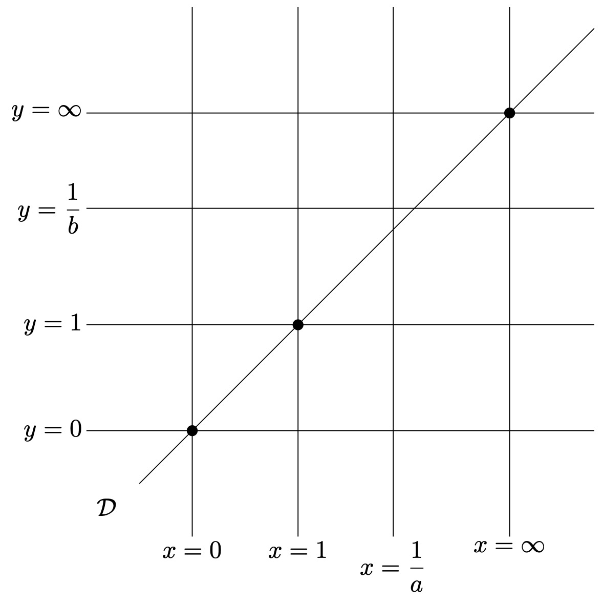
Figure 2. The figure of ${\mathcal{D}}$ on ${\mathcal{Y}}^{\circ}$

Definition-Proposition 5.4.

We define a closed subscheme ${\mathcal{C}}\subset{\mathcal{X}}^{\circ}$ as the strict transformation of $\widetilde{{\mathcal{D}}}\hookrightarrow\widetilde{{\mathcal{Y}}}^{\circ}$ by the blowing-up ${\mathcal{X}}^{\circ}\rightarrow\widetilde{{\mathcal{Y}}}^{\circ}$. The closed immersion ${\mathcal{C}}\hookrightarrow{\mathcal{X}}^{\circ}$ is described locally on $V_{0,0}^{\circ},W_{0,0}^{\circ}\subset{\mathcal{X}}^{\circ}$ as follows.

(102)

These morphisms are induced by $x\mapsto z$ and $y\mapsto z$.

By the description in Proposition 5.4 and the fact $a-b$ is invertible on $T^{\circ}$, we see that ${\mathcal{C}}$ is a conic bundle on $T^{\circ}$ with a section (e.g. $(x,y,v)=(0,0,1)$). Hence we have the following corollary.

Corollary 5.5.

The $T^{\circ}$-scheme ${\mathcal{C}}$ is isomorphic to ${\mathbb{P}}^{1}_{T^{\circ}}$.

In this subsection, we constructed the following closed subschemes.

(103)

5.2. Construction of a subgroup $\Xi^{\mathrm{can}}$ of the higher Chow group

In this section, we will construct a subgroup $\Xi^{\mathrm{can}}$ of the higher Chow group ${\mathrm{CH}}^{2}({\mathcal{X}}^{\circ},1)$. For the construction, we consider the closed subscheme ${\mathcal{C}}$ in the previous subsection and exceptional divisors $Q^{\circ}_{(0,0)},Q^{\circ}_{(1,1)}$ and $Q^{\circ}_{(\infty,\infty)}$ in Definition 3.11.

To define rational functions on them, we use the following local descriptions of $Q^{\circ}_{(0,0)},Q^{\circ}_{(1,1)}$ and $Q^{\circ}_{(\infty,\infty)}$. Since $Q^{\circ}_{(0,0)}$ and $Q^{\circ}_{(1,1)}$ are contained in $V_{0,0}$ and defined by the equation $x=y=0$ and $x=y=1$, we have the following description.

$$V^{\circ}_{0,0}\cap Q^{\circ}_{(0,0)} ={\mathrm{Spec}\,}B^{\circ}[v,x,y]/(v^{2}f(x)-g(y),x,y)\simeq{\mathrm{Spec}\,}B^{\circ}[v]$$ (104)

$$V^{\circ}_{0,0}\cap Q^{\circ}_{(1,1)} ={\mathrm{Spec}\,}B^{\circ}[v,x,y]/(v^{2}f(x)-g(y),x-1,y-1)\simeq{\mathrm{Spec}\,}B^{\circ}[v]$$

To get the local description of $Q^{\circ}_{(\infty,\infty)}$, we consider the following affine open subscheme $V^{\circ}_{1,1}$ of ${\mathcal{X}}^{\circ}$.

$$V_{1,1}^{\circ}={\mathrm{Spec}\,}B^{\circ}[v^{\prime},\xi,\eta]/((v^{\prime})^{2}\xi(\xi-1)(\xi-a)-\eta(\eta-1)(\eta-b))$$ (105)

Here $\xi=\frac{1}{x}$,$\eta=\frac{1}{y}$ and $v^{\prime}=\frac{y^{2}}{x^{2}}v$. Since $Q_{(\infty,\infty)}^{\circ}$ is defined by the equation $\xi=\eta=0$, we have the following description.

$$V^{\circ}_{1,1}\cap Q^{\circ}_{(\infty,\infty)}={\mathrm{Spec}\,}B^{\circ}[v^{\prime},\xi,\eta]/((v^{\prime})^{2}\xi(\xi-1)(\xi-a)-\eta(\eta-1)(\eta-b),\xi,\eta)\simeq{\mathrm{Spec}\,}B^{\circ}[v^{\prime}]$$ (106)

Definition-Proposition 5.6.

We define six $B^{\circ}$-rational points $p_{\bullet}^{\delta}\>(\bullet\in\{0,1,\infty\},\delta\in\{+,-\})$ on ${\mathcal{X}}^{\circ}$ as follows.

1. $p_{0}^{+}$ and $p_{0}^{-}$ correspond to $B^{\circ}$-rational points on $V_{0,0}^{\circ}\subset{\mathcal{X}}^{\circ}$ such that $(v,x,y)=\left(1,0,0\right)$ and $(v,x,y)=\left(-1,0,0\right)$ respectively.

2. $p_{1}^{+}$ and $p_{1}^{-}$ correspond to $B^{\circ}$-rational points on $V_{0,0}^{\circ}\subset{\mathcal{X}}^{\circ}$ such that $(v,x,y)=\left(\frac{\sqrt{1-b}}{\sqrt{1-a}},1,1\right)$ and $(v,x,y)=\left(-\frac{\sqrt{1-b}}{\sqrt{1-a}},1,1\right)$ respectively.

3. $p_{\infty}^{+}$ and $p_{\infty}^{-}$ correspond to $B^{\circ}$-rational points on $V_{1,1}^{\circ}\subset{\mathcal{X}}^{\circ}$ such that $(v^{\prime},\xi,\eta)=\left(\frac{\sqrt{b}}{\sqrt{a}},0,0\right)$ and $(v^{\prime},\xi,\eta)=\left(-\frac{\sqrt{b}}{\sqrt{a}},0,0\right)$ respectively.

By the local description, we have the following relations.

$${\mathcal{C}}\cap Q^{\circ}_{(0,0)}=p_{0}^{+}\sqcup p_{0}^{-},\quad{\mathcal{C}}\cap Q^{\circ}_{(1,1)}=p_{1}^{+}\sqcup p_{1}^{-},\quad{\mathcal{C}}\cap Q^{\circ}_{(\infty,\infty)}=p_{\infty}^{+}\sqcup p_{\infty}^{-}$$ (107)

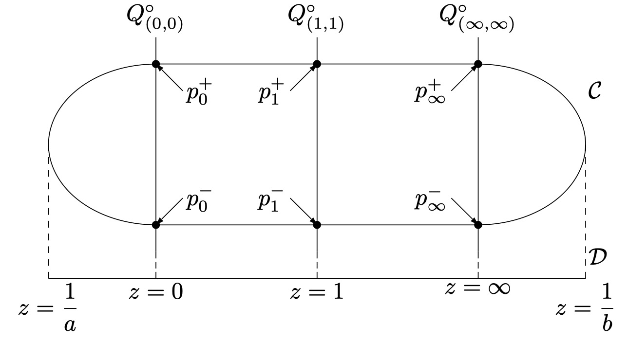
Figure 3. The relation between $p_{\bullet}^{\delta}$ and ${\mathcal{C}},Q^{\circ}_{(\bullet,\bullet)}$

Definition-Proposition 5.7.

We define the following non-zero rational functions on ${\mathcal{C}}$, $Q^{\circ}_{(0,0)}$, $Q^{\circ}_{(1,1)}$ and $Q_{(\infty,\infty)}^{\circ}$ using the local description in Proposition 5.4 and equation (104),(105).

• $\psi_{0}=(v+1)\cdot(v-1)^{-1}$, $\psi_{1}=\left(v+\frac{\sqrt{1-b}}{\sqrt{1-a}}\right)\cdot\left(v-\frac{\sqrt{1-b}}{\sqrt{1-a}}\right)^{-1}$,
  $\psi_{\infty}=\left(v+\frac{\sqrt{b}}{\sqrt{a}}\right)\cdot\left(v-\frac{\sqrt{b}}{\sqrt{a}}\right)^{-1}\in R({\mathcal{C}})^{\times}$

• $\varphi_{0}=(v-1)\cdot(v+1)^{-1}\in R\left(Q^{\circ}_{(0,0)}\right)^{\times}$

• $\varphi_{1}=\left(v-\frac{\sqrt{1-b}}{\sqrt{1-a}}\right)\cdot\left(v+\frac{\sqrt{1-b}}{\sqrt{1-a}}\right)^{-1}\in R\left(Q^{\circ}_{(1,1)}\right)^{\times}$

• $\varphi_{\infty}=\left(v^{\prime}-\frac{\sqrt{b}}{\sqrt{a}}\right)\cdot\left(v^{\prime}+\frac{\sqrt{b}}{\sqrt{a}}\right)^{-1}\in R\left(Q^{\circ}_{(\infty,\infty)}\right)^{\times}$

Then the rational functions $\varphi_{\bullet},\psi_{\bullet}$ satisfy the following relations.

1. ${\mathrm{div}}_{{\mathcal{C}}}(\psi_{0})=p_{0}^{-}-p_{0}^{+}=-{\mathrm{div}}_{Q^{\circ}_{(0,0)}}(\varphi_{0})$

2. ${\mathrm{div}}_{{\mathcal{C}}}(\psi_{1})=p_{1}^{-}-p_{1}^{+}=-{\mathrm{div}}_{Q^{\circ}_{(1,1)}}(\varphi_{1})$

3. ${\mathrm{div}}_{{\mathcal{C}}}(\psi_{\infty})=p_{\infty}^{-}-p_{\infty}^{+}=-{\mathrm{div}}_{Q^{\circ}_{(\infty,\infty)}}(\varphi_{\infty})$

Then we can construct a subgroup $\Xi^{\mathrm{can}}$ of ${\mathrm{CH}}^{2}({\mathcal{X}}^{\circ},1)$ at most rank 3 as follows.

Definition 5.8.

(Definition of $\Xi^{\mathrm{can}}$) Consider the following elements of $\bigoplus_{Z\in({\mathcal{X}}^{\circ})^{(1)}}R(Z)^{\times}$.

$$\xi_{0}=({\mathcal{C}},\psi_{0})+(Q^{\circ}_{(0,0)},\varphi_{0})$$ (108)

$$\xi_{1}=({\mathcal{C}},\psi_{1})+(Q^{\circ}_{(1,1)},\varphi_{1})$$

$$\xi_{\infty}=({\mathcal{C}},\psi_{\infty})+(Q^{\circ}_{(\infty,\infty)},\varphi_{\infty})$$

By Proposition 5.7, they are in ${\mathrm{Ker}}\left(\bigoplus_{Z\in({\mathcal{X}}^{\circ})^{(1)}}R(Z)^{\times}\xrightarrow{{\mathrm{div}}}\bigoplus_{p\in({\mathcal{X}}^{\circ})^{(2)}}{\mathbb{Z}}\cdot p\right)$. Hence these elements define elements in ${\mathrm{CH}}^{2}({\mathcal{X}}^{\circ},1)$ which are denoted by the same symbols $\xi_{0},\xi_{1},\xi_{\infty}$ respectively. We define $\Xi^{\mathrm{can}}\subset{\mathrm{CH}}^{2}({\mathcal{X}}^{\circ},1)$ to be the subgroup generated by $\xi_{0},\xi_{1}$ and $\xi_{\infty}$. For $\epsilon\in{\mathbb{Z}}^{\{0,1,\infty\}}$, we set

$$\xi(\epsilon)=\epsilon(0)\xi_{0}+\epsilon(1)\xi_{1}+\epsilon(\infty)\xi_{\infty}\in\Xi^{\mathrm{can}}.$$ (109)

By the following pull-back map, we can regard an element $\xi\in{\mathrm{CH}}^{2}({\mathcal{X}}^{\circ},1)$ as a family of higher Chow cycles $\{\xi_{t}\}_{t\in T^{\circ}}$. The existence of the following pull-back map is given in [Lev98], Part I, Chapter II, 2.1.6.

Definition 5.9.

For a $k$-rational point $t\in T^{\circ}(k)$, $i_{t}:{\mathcal{X}}_{t}\rightarrow{\mathcal{X}}^{\circ}$ in Definition 4.23 is a $k$-morphism between smooth varieties. Hence we have a pull-back map

$$i_{t}^{*}:{\mathrm{CH}}^{2}({\mathcal{X}}^{\circ},1)\>{\longrightarrow}\>{\mathrm{CH}}^{2}({\mathcal{X}}_{t},1).$$ (110)

For each $\xi\in{\mathrm{CH}}^{2}({\mathcal{X}}^{\circ},1)$, $i_{t}^{*}\xi$ is denoted by $\xi_{t}$.

Proposition 5.10.

For a $k$-rational point $t\in T^{\circ}(k)$ and $\epsilon\in{\mathbb{Z}}^{\{0,1,\infty\}}$, $\xi(\epsilon)_{t}\in{\mathrm{CH}}^{2}({\mathcal{X}}_{t},1)$ is represented by the following element in $\bigoplus_{Z\in{\mathcal{X}}_{t}^{(1)}}R(Z)^{\times}$.

$$\left({\mathcal{C}}_{t},(\psi_{0})_{t}^{\epsilon(0)}(\psi_{1})_{t}^{\epsilon(1)}(\psi_{\infty})_{t}^{\epsilon(\infty)}\right)$$ (111)

$$+(Q_{(0,0)t},(\varphi_{0})^{\epsilon(0)}_{t})+(Q_{(1,1)t},(\varphi_{1})^{\epsilon(1)}_{t})+(Q_{(\infty,\infty)t},(\varphi_{\infty})^{\epsilon(\infty)}_{t})$$

Here ${\mathcal{C}}_{t},Q_{(\bullet,\bullet)t}$ are the fibers of ${\mathcal{C}}$ and $Q_{(\bullet,\bullet)}^{\circ}$ at $t$ and $(\psi_{\bullet})_{t},(\varphi_{\bullet})_{t}$ are the pull back of the rational function $\psi_{\bullet},\varphi_{\bullet}$ by ${\mathcal{C}}_{t}\hookrightarrow{\mathcal{C}}$ and $Q_{(\bullet,\bullet)t}\hookrightarrow Q_{(\bullet,\bullet)}^{\circ}$.

Proof.

Recall that we regard elements in $\bigoplus_{Z\in({\mathcal{X}}^{\circ})^{(1)}}R(Z)^{\times}$ as elements in $Z^{2}({\mathcal{X}}^{\circ},1)$ $\subset Z^{2}({\mathcal{X}}^{\circ}\times_{k}\Delta^{1})$ ($\Delta^{1}={\mathrm{Spec}\,}k[T_{0},T_{1}]/(T_{0}+T_{1}-1)$) by considering their graphs of rational functions. For example, $({\mathcal{C}},\psi_{1})$ represents a codimension 1 integral closed subscheme of ${\mathcal{C}}\times_{k}\Delta^{1}$ defined by the local equation

$$\left(v-\frac{\sqrt{1-b}}{\sqrt{1-a}}\right)T_{0}+\left(v+\frac{\sqrt{1-b}}{\sqrt{1-a}}\right)T_{1}=0.$$ (112)

Here we use the local coordinates of ${\mathcal{C}}$ in Proposition 5.4. This closed subscheme intersect properly with ${\mathcal{X}}_{t}\times_{k}\Delta^{1},{\mathcal{X}}_{t}\times_{k}\{T_{0}=0\},{\mathcal{X}}_{t}\times_{k}\{T_{1}=0\}$. Hence the pull-back of the cycle corresponding to $({\mathcal{C}},\psi_{1})$ by ${\mathcal{X}}_{t}\hookrightarrow{\mathcal{X}}^{\circ}$ is defined. The pull-back coincides with the intersection of this closed subscheme with ${\mathcal{X}}_{t}\times_{k}\Delta^{1}$ and the intersection is the graph of $(\psi_{1})_{t}$. By considering pull-backs of $({\mathcal{C}},\psi_{\bullet})$ and $(Q^{\circ}_{(\bullet,\bullet)},\varphi_{\bullet})$ for $\bullet=0,1,\infty$ similarly, we can show that

$$({\mathcal{C}}_{t},(\psi_{0})_{t})+(Q_{(0,0),t},(\varphi_{0})_{t})$$ (113)

$$({\mathcal{C}}_{t},(\psi_{1})_{t})+(Q_{(1,1),t},(\varphi_{1})_{t})$$

$$({\mathcal{C}}_{t},(\psi_{\infty})_{t})+(Q_{(\infty,\infty),t},(\varphi_{\infty})_{t})$$

represents $\xi_{0,t},\xi_{1,t}$ and $\xi_{\infty,t}\in{\mathrm{CH}}^{2}({\mathcal{X}}_{t},1)$. Hence we have the result. ∎

5.3. Definition of a subgroup $\Xi$ of the higher Chow group

In this section, we define $\Xi\subset{\mathrm{CH}}^{2}({\mathcal{X}}^{\circ},1)$ and give representatives in $\bigoplus_{Z\in({\mathcal{X}}^{\circ})^{(1)}}R(Z)^{\times}$ for cycles in $\Xi$. In Section 6, we use these expressions to show that a subgroup $\widetilde{I}$ of $\widetilde{G}$ stabilize $\Xi^{\mathrm{can}}\subset{\mathrm{CH}}^{2}({\mathcal{X}}^{\circ},1)$.

Definition 5.11.

We define a subgroup $\Xi$ of ${\mathrm{CH}}^{2}({\mathcal{X}}^{\circ},1)$ as

$$\Xi=\sum_{\widetilde{\rho}\in\widetilde{G}}\widetilde{\rho}_{*}\Xi^{\mathrm{can}}$$ (114)

where $\Xi^{\mathrm{can}}\subset{\mathrm{CH}}^{2}({\mathcal{X}}^{\circ},1)$ is the subgroup of higher Chow group defined in Definition 5.8 and $\widetilde{\rho}_{*}:{\mathrm{CH}}^{2}({\mathcal{X}}^{\circ},1)\rightarrow{\mathrm{CH}}^{2}({\mathcal{X}}^{\circ},1)$ is the push-forward map induced by an automorphism $\widetilde{\rho}:{\mathcal{X}}^{\circ}\rightarrow{\mathcal{X}}^{\circ}$. For a $k$-rational point $t\in T^{\circ}(k)$, we define $\Xi_{t}\subset{\mathrm{CH}}^{2}({\mathcal{X}}_{t},1)$ as the image of $\Xi$ under $i_{t}^{*}$ in Definition 5.9.

Definition 5.12.

For $\rho\in G$, we define a closed subscheme ${\mathcal{D}}_{\rho}\subset{\mathcal{Y}}^{\circ}$ by the schematic image $\rho({\mathcal{D}})$. Note that ${\mathcal{D}}_{\rho}$ is determined by the image of $\rho\in G$ under $G\rightarrow G_{0}$. The local equation of ${\mathcal{D}}_{\rho}$ is given by $(\rho^{-1})^{\sharp}(x-y)=0$.

We define $\widetilde{{\mathcal{D}}}_{\rho}\hookrightarrow\widetilde{{\mathcal{Y}}}^{\circ}$ as the pull-back of ${\mathcal{D}}_{\rho}\hookrightarrow{\mathcal{Y}}^{\circ}$ by $\widetilde{{\mathcal{Y}}}^{\circ}\rightarrow{\mathcal{Y}}^{\circ}$. Furthermore, we define ${\mathcal{C}}_{\rho}\hookrightarrow{\mathcal{X}}^{\circ}$ as the strict transformation of $\widetilde{{\mathcal{D}}}_{\rho}$ by ${\mathcal{X}}^{\circ}\rightarrow\widetilde{{\mathcal{Y}}}^{\circ}$.

(115)

Since $\rho({\mathcal{D}})={\mathcal{D}}_{\rho}$, for $\widetilde{\rho}\in\widetilde{G}$, we have $\widetilde{\rho}(\widetilde{{\mathcal{D}}})=\widetilde{{\mathcal{D}}}_{\rho}$ and $\widetilde{\rho}({\mathcal{C}})={\mathcal{C}}_{\rho}$.

The following proposition follows from Proposition 4.21 and Definition 5.12.

Proposition 5.13.

By an automorphism $\widetilde{\rho}=(\rho,\zeta)\in\widetilde{G}$ on ${\mathcal{X}}^{\circ}$, we have

$$\widetilde{\rho}({\mathcal{C}})={\mathcal{C}}_{\rho},\quad\widetilde{\rho}(Q^{\circ}_{(0,0)})=Q^{\circ}_{\rho\cdot(0,0)},\quad\widetilde{\rho}(Q^{\circ}_{(1,1)})=Q^{\circ}_{\rho\cdot(1,1)},\quad\widetilde{\rho}(Q^{\circ}_{(\infty,\infty)})=Q^{\circ}_{\rho\cdot(\infty,\infty)}.$$ (116)

Let $\epsilon\in{\mathbb{Z}}^{\{0,1,\infty\}}$. Then $\rho_{*}\xi(\epsilon)\in{\mathrm{CH}}^{2}({\mathcal{X}}^{\circ},1)$ is represented by the following elements in $\bigoplus_{Z\in({\mathcal{X}}^{\circ})^{(1)}}R(Z)^{\times}$.

$$\left({\mathcal{C}}_{\rho},(\widetilde{\rho}^{-1})^{\sharp}(\psi_{0}^{\epsilon(0)}\psi_{1}^{\epsilon(1)}\psi_{\infty}^{\epsilon(\infty)})\right)+(Q_{\rho\cdot(0,0)}^{\circ},(\widetilde{\rho}^{-1})^{\sharp}(\varphi_{0}^{\epsilon(0)}))$$ (117)

$$+(Q_{\rho\cdot(1,1)}^{\circ},(\widetilde{\rho}^{-1})^{\sharp}(\varphi_{1}^{\epsilon(1)}))+(Q_{\rho\cdot(\infty,\infty)}^{\circ},(\widetilde{\rho}^{-1})^{\sharp}(\varphi_{\infty}^{\epsilon(\infty)}))$$

where $(\widetilde{\rho}^{-1})^{\sharp}$ are the field isomorphisms $R({\mathcal{C}})\rightarrow R({\mathcal{C}}_{\rho})$ and $R(Q_{(\bullet,\bullet)}^{\circ})\rightarrow R(Q_{\rho\cdot(\bullet,\bullet)}^{\circ})$ induced by $\widetilde{\rho}$.

Remark 5.14.

As we stated in the introduction, several elements in $\widetilde{\rho}_{*}\Xi^{\mathrm{can}}$ are at first constructed geometrically after T. Terasoma’s idea. The keys for the geometric construction are the following.

1. There exists the isomorphism ${\mathcal{C}}_{\rho}\simeq{\mathbb{P}}^{1}_{T^{\circ}}$ over $T^{\circ}$.

2. For $\bullet=0,1,\infty$, ${\mathcal{C}}_{\rho}\cap Q_{\rho\cdot(\bullet,\bullet)}^{\circ}$ decompose into the disjoint union of two $B^{\circ}$-rational points.

From these facts, we can construct higher Chow cycles in $\Xi$ directly by the similar method in subsection 5.2.

6. Subgroups $\widetilde{I}$ and $\widetilde{G}_{\mathrm{fib}}$ of $\widetilde{G}$

In this section, we construct two subgroups $\widetilde{I}$ and $\widetilde{G}_{\mathrm{fib}}$ of $\widetilde{G}$. As we will see later (Proposition 9.12), these subgroups stabilize the image of $\Xi\subset{\mathrm{CH}}^{2}({\mathcal{X}}^{\circ},1)$ under the transcendental regulator maps at fibers ${\mathcal{X}}_{t}$.

The subgroup $\widetilde{I}$ consists of automorphisms in $\widetilde{G}$ which stabilize a subgroup of symbols in $\bigoplus_{Z\in({\mathcal{X}}^{\circ})^{(1)}}R(Z)^{\times}$ which represents cycles in $\Xi^{\mathrm{can}}$. Hence $\widetilde{I}$ stabilize $\Xi^{\mathrm{can}}$ (Proposition 6.8). We describe the explicit $\widetilde{I}$-action on $\Xi^{\mathrm{can}}$.

The subgroup $\widetilde{G}_{\mathrm{fib}}$ consists of automorphisms in $\widetilde{G}$ over $T^{\circ}$. Hence elements of $\widetilde{G}_{\mathrm{fib}}$ induce automorphisms of each fiber ${\mathcal{X}}_{t}$. Since $\widetilde{G}_{\mathrm{fib}}$ acts on a relative 2-form $\omega\in\Gamma({\mathcal{X}}^{\circ},\Omega^{2}_{{\mathcal{X}}^{\circ}/T^{\circ}})$ by the multiplication $\pm 1$, $\widetilde{G}_{\mathrm{fib}}$ stabilize the image of the transcendental regulator map (Proposition 9.12).

6.1. Definition of $\widetilde{I}$ and stability of $\Xi^{\mathrm{can}}$ under the $\widetilde{I}$-action

Definition 6.1.

By Proposition 4.3, we identify $H_{0}=\mathfrak{S}(\{0,1,1/c,\infty\})$. We define a subgroup $I_{0}\subset G_{0}$ by the image of the stabilizer of $1/c\in\{0,1,1/c,\infty\}$ under the following diagonal embedding.

(118)

Consider the following diagram.

(119)

By the description of $H_{0}\rightarrow\underline{H}_{0}$ in Remark 4.5 and the commutativity of diagram (119), $I_{0}\hookrightarrow G_{0}\twoheadrightarrow\underline{G}_{0}$ is injective and its image coincides with the image of the diagonal embedding of $\underline{H}_{0}$. We denote the image of $I_{0}$ in $\underline{G}_{0}$ by $\underline{I}_{0}$. By the argument above, $I_{0}\simeq\underline{I}_{0}$.

Remark 6.2.

An element of the stabilizer of $1/c$ induces a permutation on $\{0,1,\infty\}\subset\{0,1,1/c,\infty\}$. Hence we often identify $I_{0}$ with $\mathfrak{S}(\{0,1,\infty\})$. For each $\rho_{0}\in I_{0}=\mathfrak{S}(\{0,1,\infty\})$, the action of $\rho_{0}$ on ${\mathcal{Y}}$ is given in the following Table 5.

Table 5. The action of $I_{0}=\mathfrak{S}(\{0,1,\infty\})$ on ${\mathcal{Y}}$

$\rho_{0}$	$(\underline{\rho}_{0}^{\sharp}(a),\underline{\rho}_{0}^{\sharp}(b))$	$(\rho_{0}^{\sharp}(x),\rho_{0}^{\sharp}(y))$	$\rho_{0}$	$(\underline{\rho}_{0}^{\sharp}(a),\underline{\rho}_{0}^{\sharp}(b))$	$(\rho_{0}^{\sharp}(x),\rho_{0}^{\sharp}(y))$
${\mathrm{id}}$	$(a,b)$	$(x,y)$	$(0\;1)$	$(\frac{a}{a-1},\frac{b}{b-1})$	$(1-x,1-y)$
$(1\;\infty)$	$(1-a,1-b)$	$(\frac{x}{x-1},\frac{y}{y-1})$	$(0\;1\;\infty)$	$(\frac{a-1}{a},\frac{b-1}{b})$	$(\frac{1}{1-x},\frac{1}{1-y})$
$(0\;\infty)$	$(\frac{1}{a},\frac{1}{b})$	$(\frac{1}{x},\frac{1}{y})$	$(0\;\infty\;1)$	$(\frac{1}{1-a},\frac{1}{1-b})$	$(\frac{x-1}{x},\frac{y-1}{y})$

Definition 6.3.

We define subgroups $\underline{I}\subset\underline{G}$, $I\subset G$ and $\widetilde{I}\subset\widetilde{G}$ as follows.

$$\underline{I}=\{\underline{\rho}\in\underline{G}:\underline{\rho}_{0}\in\underline{I}_{0}\}$$ (120)

$$I=\{\rho\in G:\rho_{0}\in I_{0}\}$$

$$\widetilde{I}=\{(\rho,\zeta)\in\widetilde{G}:\rho\in I\}$$

Then $I$ is isomorphic to $I_{0}\times_{\underline{I}_{0}}\underline{I}$. Since $I_{0}\rightarrow\underline{I}_{0}$ is an isomorphism by Definition 6.1, $I\rightarrow\underline{I}$ is also an isomorphism.

Remark 6.4.

Since $\underline{I}_{0}\subset\underline{G}_{0}$ is the image of diagonal embedding (Definition 6.1), we have

$$\underline{I}=\{(\underline{\rho}^{(1)},\underline{\rho}^{(2)})\in\underline{H}\times\underline{H}:\underline{\rho}_{0}^{(1)}=\underline{\rho}_{0}^{(2)}\}=\underline{H}\times_{\underline{H}_{0}}\underline{H}$$ (121)

Since $\underline{H}\simeq\mathfrak{S}_{4}$ by Remark 4.8 and $\underline{H}_{0}\simeq\mathfrak{S}_{3}$ by Definition 4.1, $\underline{I}$ is isomorphic to $\mathfrak{S}_{4}\times_{\mathfrak{S}_{3}}\mathfrak{S}_{4}$. Since $I\simeq\underline{I}$, $I$ is also isomorphic to $\mathfrak{S}_{4}\times_{\mathfrak{S}_{3}}\mathfrak{S}_{4}$. Furthermore, since ${\mathrm{sgn}}(\underline{\rho}_{0}^{(1)}){\mathrm{sgn}}(\underline{\rho}_{0}^{(2)})=1$ for $\rho\in I$, we have a splitting of $\widetilde{I}\rightarrow I$ defined by $I\rightarrow\widetilde{I};\rho\mapsto(\rho,1)$. By this splitting, we have an isomorphism $\widetilde{I}\simeq I\times{\mathbb{Z}}/2{\mathbb{Z}}$.

We will show that the $\widetilde{I}$-action stabilizes $\Xi^{\mathrm{can}}\subset{\mathrm{CH}}^{2}({\mathcal{X}}^{\circ},1)$. Hereafter in this subsection, we assume $\widetilde{\rho}=(\rho,\zeta)\in\widetilde{I}$. To prove $\widetilde{\rho}_{*}\Xi^{\mathrm{can}}\subset\Xi^{\mathrm{can}}$, we show that the symbol in Proposition 5.13 which represents $\widetilde{\rho}_{*}\xi(\epsilon)$ coincides with the symbol which represents an element in $\Xi^{\mathrm{can}}$.

Proposition 6.5.

1. Let ${\mathcal{C}}_{\rho}$ be the closed subscheme defined in Definition 5.12. Then we have ${\mathcal{C}}_{\rho}={\mathcal{C}}$.

2. Let $\rho_{0}$ be the image of $\rho$ by $I\rightarrow I_{0}\xrightarrow{\sim}\mathfrak{S}(\{0,1,\infty\})$ where the last isomorphism is the one in Remark 6.2. Then we have the following.

   $$Q^{\circ}_{\rho\cdot(0,0)}=Q^{\circ}_{(\rho_{0}(0),\rho_{0}(0))},\quad Q^{\circ}_{\rho\cdot(1,1)}=Q^{\circ}_{(\rho_{0}(1),\rho_{0}(1))},\quad Q^{\circ}_{\rho\cdot(\infty,\infty)}=Q^{\circ}_{(\rho_{0}(\infty),\rho_{0}(\infty))}$$ (122)

Proof.

By the description of $I_{0}$-action in Table 5, the $I$-action on ${\mathcal{Y}}^{\circ}$ stabilizes the local equation $x=y$ of ${\mathcal{D}}$. Hence ${\mathcal{D}}_{\rho}={\mathcal{D}}$ and by Definition 5.12, we have (1). (2) follows from the way of the identification $I_{0}=\mathfrak{S}(\{0,1,\infty\})$ in Remark 6.2. ∎

We will prove that the sets of rational functions $\{\varphi_{\bullet}^{\pm 1}:\bullet=0,1,\infty\}$ and $\{\psi_{\bullet}^{\pm 1}:\bullet=0,1,\infty\}$ are stable under the $\widetilde{I}$-action.

Definition-Proposition 6.6.

By Proposition 6.5, we have

$$\widetilde{\rho}(p^{+}_{\bullet})\sqcup\widetilde{\rho}(p^{-}_{\bullet})=\widetilde{\rho}({\mathcal{C}}\cap Q^{\circ}_{(\bullet,\bullet)})={\mathcal{C}}\cap Q^{\circ}_{(\rho_{0}(\bullet),\rho_{0}(\bullet))}=p^{+}_{\rho_{0}(\bullet)}\sqcup p^{-}_{\rho_{0}(\bullet)}$$ (123)

for $\bullet=0,1,\infty$ where $p^{+}_{\bullet},p^{-}_{\bullet}$ are $B^{\circ}$-rational points in Definition 5.6. Then by comparing connected components in $(\ref{intersectionpoints})$, we have either

$$\mathrm{(A)}\left\{\begin{aligned} &\widetilde{\rho}(p^{+}_{\bullet})=p^{+}_{\rho_{0}(\bullet)}\\ &\widetilde{\rho}(p^{-}_{\bullet})=p^{-}_{\rho_{0}(\bullet)}\end{aligned}\right.\quad\text{or}\quad\mathrm{(B)}\left\{\begin{aligned} &\widetilde{\rho}(p^{+}_{\bullet})=p^{-}_{\rho_{0}(\bullet)}\\ &\widetilde{\rho}(p^{-}_{\bullet})=p^{+}_{\rho_{0}(\bullet)}\end{aligned}\right.$$ (124)

for $\bullet=0,1,\infty$. We define $\delta(\widetilde{\rho})\in\{\pm 1\}^{\{0,1,\infty\}}$ as follows.

• If the case $\mathrm{(A)}$ occurs for $\bullet=0$, $\delta(\widetilde{\rho})(\rho_{0}(0))=1$, else $\delta(\widetilde{\rho})(\rho_{0}(0))=-1$.

• If the case $\mathrm{(A)}$ occurs for $\bullet=1$, $\delta(\widetilde{\rho})(\rho_{0}(1))=1$, else $\delta(\widetilde{\rho})(\rho_{0}(1))=-1$.

• If the case $\mathrm{(A)}$ occurs for $\bullet=\infty$, $\delta(\widetilde{\rho})(\rho_{0}(\infty))=1$, else $\delta(\widetilde{\rho})(\rho_{0}(\infty))=-1$.

Then we have the following.

1. For $\bullet=0,1,\infty$, we have the following.

   $$(\widetilde{\rho}^{-1})^{\sharp}(\psi_{\bullet})=\psi_{\rho_{0}(\bullet)}^{\delta(\widetilde{\rho})(\rho_{0}(\bullet))},\quad(\widetilde{\rho}^{-1})^{\sharp}(\varphi_{\bullet})=\varphi_{\rho_{0}(\bullet)}^{\delta(\widetilde{\rho})(\rho_{0}(\bullet))}$$ (125)

2. We define an $\widetilde{I}$-action on $\{\pm 1\}^{\{0,1,\infty\}}$ by

   (126)

   Then the map $\delta:\widetilde{I}\rightarrow\{\pm 1\}^{\{0,1,\infty\}};\widetilde{\rho}\mapsto\delta(\widetilde{\rho})$ defines a 1-cocycle with respect to this $\widetilde{I}$-action.

To prove this proposition, we use the following lemma.

Lemma 6.7.

Let $\varphi_{1},\varphi_{2}\in R({\mathbb{P}}^{1}_{T^{\circ}})^{\times}$. Assume $\varphi_{1}\not\in{\mathrm{Frac}}(B^{\circ})$. Suppose that ${\mathrm{div}}(\varphi_{1})={\mathrm{div}}(\varphi_{2})$ and ${\mathrm{div}}(\varphi_{1}+1)={\mathrm{div}}(\varphi_{2}+1)$. Then we have $\varphi_{1}=\varphi_{2}$.

Proof.

Since ${\mathbb{P}}^{1}_{T^{\circ}}$ is normal, ${\mathrm{div}}(\varphi_{1})={\mathrm{div}}(\varphi_{2})$ and ${\mathrm{div}}(\varphi_{1}+1)={\mathrm{div}}(\varphi_{2}+1)$ imply that there exist $p,q\in\Gamma({\mathbb{P}}^{1}_{T^{\circ}},{\mathcal{O}}_{{\mathbb{P}}^{1}_{T^{\circ}}}^{\times})=(B^{\circ})^{\times}$ such that $\varphi_{1}=p\varphi_{2}$ and $1+\varphi_{1}=q(1+\varphi_{2})$. Thus $(1-q)+(1-qp^{-1})\varphi_{1}=0$. Since $\varphi_{1}\not\in{\mathrm{Frac}}(B^{\circ})$, we have $p=q=1$. i.e. $\varphi_{1}=\varphi_{2}$. ∎

Proof.

(Proposition 6.6) Note that ${\mathcal{C}}$ and $Q^{\circ}_{(\bullet,\bullet)}$ are isomorphic to ${\mathbb{P}}^{1}_{T^{\circ}}$ (Corollary 5.5). By the explicit presentations for $\varphi_{\bullet},\psi_{\bullet}$ in Definition 5.7, we see that $\varphi_{\bullet}^{\pm 1},\psi_{\bullet}^{\pm 1}\not\in{\mathrm{Frac}}(B^{\circ})$. Hence we can use Lemma 6.7. By the definition of $\delta$, we have the following relations for $\bullet=0,1,\infty$.

$${\mathrm{div}}_{{\mathcal{C}}}((\widetilde{\rho}^{-1})^{\sharp}(\psi_{\bullet}))={\mathrm{div}}_{{\mathcal{C}}}(\psi_{\rho_{0}(\bullet)}^{\delta(\widetilde{\rho})(\rho_{0}(\bullet))})$$ (127)

$${\mathrm{div}}_{Q^{\circ}_{(\rho_{0}(\bullet),\rho_{0}(\bullet))}}((\widetilde{\rho}^{-1})^{\sharp}(\varphi_{\bullet}))={\mathrm{div}}_{Q^{\circ}_{(\rho_{0}(\bullet),\rho_{0}(\bullet))}}(\varphi_{\rho_{0}(\bullet)}^{\delta(\widetilde{\rho})(\rho_{0}(\bullet))})$$

Here we use the relations in Proposition 5.7. Next, we see the divisors associated with $1+\varphi_{\bullet}$ and $1+\psi_{\bullet}$. We will consider a closed subscheme ${\mathcal{Z}}\subset{\mathcal{X}}^{\circ}$ defined by the local equation $v=0$. Then we have $B^{\circ}$-rational points $q_{c},q_{0},q_{1},q_{\infty}$ on ${\mathcal{X}}^{\circ}$ such that

$$q_{c}={\mathcal{Z}}\cap{\mathcal{C}},\quad q_{\bullet}={\mathcal{Z}}\cap Q_{(\bullet,\bullet)}^{\circ}\quad(\bullet=0,1,\infty).$$ (128)

Using these $B^{\circ}$-rational points, we can describe the divisors of $1+\psi_{\bullet}^{\pm 1}$ and $1+\varphi_{\bullet}^{\pm 1}$ as follows.

$$\left\{\begin{aligned} &{\mathrm{div}}_{{\mathcal{C}}}(1+\psi_{\bullet})=q_{c}-p_{\bullet}^{+}\\ &{\mathrm{div}}_{{\mathcal{C}}}(1+\psi_{\bullet}^{-1})=q_{c}-p_{\bullet}^{-}\\ \end{aligned}\right.,\quad\left\{\begin{aligned} &{\mathrm{div}}_{Q^{\circ}_{(\bullet,\bullet)}}(1+\varphi_{\bullet})=q_{\bullet}-p_{\bullet}^{-}\\ &{\mathrm{div}}_{Q^{\circ}_{(\bullet,\bullet)}}(1+\varphi_{\bullet}^{-1})=q_{\bullet}-p_{\bullet}^{+}\\ \end{aligned}\right.$$ (129)

where $\bullet=0,1,\infty$. This follows from the explicit presentations of Definition 5.7. By the explicit description of $\widetilde{G}$-action in Proposition 4.20, we see that the closed subscheme ${\mathcal{Z}}\subset{\mathcal{X}}^{\circ}$ is stable under the $\widetilde{I}$-action. Then we have

$$\widetilde{\rho}(q_{c})=\widetilde{\rho}({\mathcal{Z}}\cap{\mathcal{C}})={\mathcal{Z}}\cap{\mathcal{C}}=q_{c}$$ (130)

$$\widetilde{\rho}(q_{\bullet})=\widetilde{\rho}({\mathcal{Z}}\cap Q^{\circ}_{(\bullet,\bullet)})={\mathcal{Z}}\cap Q^{\circ}_{(\rho_{0}(\bullet),\rho_{0}(\bullet))}=q_{\rho_{0}(\bullet)}$$

By the definition of $\delta(\rho)(\bullet)$, we have the following relations for $\bullet=0,1,\infty$.

$${\mathrm{div}}_{{\mathcal{C}}}(1+(\widetilde{\rho}^{-1})^{\sharp}(\psi_{\bullet}))=q_{c}-\widetilde{\rho}(p_{\bullet}^{+})={\mathrm{div}}_{{\mathcal{C}}}(1+\psi_{\rho_{0}(\bullet)}^{\delta(\widetilde{\rho})(\rho_{0}(\bullet))})$$ (131)

$${\mathrm{div}}_{Q^{\circ}_{(\rho_{0}(\bullet),\rho_{0}(\bullet))}}(1+(\widetilde{\rho}^{-1})^{\sharp}(\varphi_{\bullet}))=q_{\rho_{0}(\bullet)}-\widetilde{\rho}(p^{-}_{\bullet})={\mathrm{div}}_{Q^{\circ}_{(\rho_{0}(\bullet),\rho_{0}(\bullet))}}(1+\varphi_{\rho_{0}(\bullet)}^{\delta(\widetilde{\rho})(\rho_{0}(\bullet))})$$

By (127) and (131), we have (1). (2) follows from (1). ∎

Proposition 6.8.

We have $\widetilde{\rho}_{*}(\Xi^{\mathrm{can}})=\Xi^{\mathrm{can}}$. The $\widetilde{I}$-action on $\Xi^{\mathrm{can}}$ is given as follows:

(132)

where $\delta(\widetilde{\rho})\cdot(\epsilon\circ\rho_{0}^{-1})$ denotes the product of functions $\delta(\widetilde{\rho})\in\{\pm 1\}^{\{0,1,\infty\}}\subset{\mathbb{Z}}^{\{0,1,\infty\}}$ and $\epsilon\circ\rho_{0}^{-1}\in{\mathbb{Z}}^{\{0,1,\infty\}}$.

Proof.

By Proposition 6.6, $\left({\mathcal{C}}_{\rho},\prod_{\bullet=0,1,\infty}(\widetilde{\rho}^{-1})^{\sharp}(\psi_{\bullet})^{\epsilon(\bullet)}\right)=\left({\mathcal{C}},\prod_{\bullet=0,1,\infty}\psi_{\bullet}^{\delta(\widetilde{\rho})(\bullet)\cdot\epsilon(\rho_{0}^{-1}(\bullet))}\right)$ and $\left(Q^{\circ}_{\rho\cdot(\bullet,\bullet)},(\widetilde{\rho}^{-1})^{\sharp}\left(\varphi_{\bullet}\right)^{\epsilon(\bullet)}\right)=\left(Q^{\circ}_{(\rho_{0}(\bullet),\rho_{0}(\bullet))},\varphi_{\bullet}^{\delta(\widetilde{\rho})(\rho_{0}(\bullet))\cdot\epsilon(\bullet)}\right)$ for $\bullet=0,1,\infty$. Therefore, we have $\widetilde{\rho}_{*}\xi(\epsilon)=\xi\left(\delta(\widetilde{\rho})\cdot(\epsilon\circ\rho_{0}^{-1})\right)$ by Proposition 5.13. Hence we have the result. ∎

Example 6.9.

We calculate $\delta,\underline{\chi}^{(i)}$ for some elements in $\widetilde{I}$. The result will be used in Section 9. For the calculation, we use the local description of $\widetilde{G}$-action on ${\mathcal{X}}^{\circ}$ in Proposition 4.20. Since $I\rightarrow\underline{I}$ is an isomorphism (Defintion 6.3), to specify elements in $I$, it is enough to give an automorphism on $B^{\circ}$ which belongs to $\underline{I}$.

1. Let $\widetilde{\rho}^{a}=(\rho^{a},1)\in\widetilde{I}$ be the element satisfying that

   $$(\underline{\rho}^{a})^{\sharp}:B^{\circ}\rightarrow B^{\circ};\quad\sqrt{a},\sqrt{1-a},\sqrt{b},\sqrt{1-b}\mapsto\sqrt{a},-\sqrt{1-a},\sqrt{b},\sqrt{1-b}.$$ (133)

   Then we have $\rho_{0}^{a}={\mathrm{id}}\in I=\mathfrak{S}(\{0,1,\infty\})$, $\chi^{(1)}(\underline{\rho}^{a})=-1$ and $\chi^{(2)}(\underline{\rho}^{a})=1$. Furthermore, $\delta(\widetilde{\rho}^{a})$ can be computed as

   $$\delta(\widetilde{\rho}^{a})(0)=-1,\quad\delta(\widetilde{\rho}^{a})(1)=1,\quad\delta(\widetilde{\rho}^{a})(\infty)=-1.$$ (134)

2. Let $\widetilde{\rho}^{b}=(\rho^{b},1)\in\widetilde{I}$ be the element satisfying that

   $$(\underline{\rho}^{a})^{\sharp}:B^{\circ}\rightarrow B^{\circ};\quad\sqrt{a},\sqrt{1-a},\sqrt{b},\sqrt{1-b}\mapsto\sqrt{1-a},\sqrt{a},\sqrt{1-b},\sqrt{b}.$$ (135)

   Then we have $\rho_{0}^{b}=(1\>\infty)\in I_{0}=\mathfrak{S}(\{0,1,\infty\})$, $\chi^{(1)}(\underline{\rho}^{b})=1$ and $\chi^{(2)}(\underline{\rho}^{b})=1$. Furthermore, $\delta(\widetilde{\rho}^{a})$ can be computed as

   $$\delta(\widetilde{\rho}^{a})(0)=-1,\quad\delta(\widetilde{\rho}^{a})(1)=-1,\quad\delta(\widetilde{\rho}^{a})(\infty)=-1.$$ (136)

6.2. A fiber-preserving subgroup $\widetilde{G}_{\mathrm{fib}}$ of $\widetilde{G}$

In this section, we define another subgroup $\widetilde{G}_{\mathrm{fib}}$ of $\widetilde{G}$.

Definition-Proposition 6.10.

We define a normal subgroup $\widetilde{G}_{\mathrm{fib}}\subset\widetilde{G}$ as

$$\widetilde{G}_{\mathrm{fib}}={\mathrm{Ker}}(\widetilde{G}\rightarrow\underline{G}).$$ (137)

In other words, $\widetilde{G}_{\mathrm{fib}}$ consists of elements in $\widetilde{G}\subset{\mathrm{Aut}}_{k}({\mathcal{X}}^{\circ})$ which are automorphisms over $T^{\circ}$. Then we have $\widetilde{G}_{\mathrm{fib}}\simeq({\mathbb{Z}}/2{\mathbb{Z}})^{5}$.

Proof.

First, we show ${\mathrm{Ker}}(H\rightarrow\underline{H})\simeq{\mathrm{Ker}}(H_{0}\rightarrow\underline{H}_{0})\simeq({\mathbb{Z}}/2{\mathbb{Z}})^{2}$. We have the first isomorphism by the fact that a fiber product preserves kernels and the second isomorphism follows from Table 2. Hence we have ${\mathrm{Ker}}(G\rightarrow\underline{G})\simeq({\mathbb{Z}}/2{\mathbb{Z}})^{4}$. Since $\underline{\rho}^{(1)}_{0}=\underline{\rho}^{(2)}_{0}={\mathrm{id}}_{\underline{H}_{0}}$ for $\rho=(\rho^{(1)},\rho^{(2)})\in{\mathrm{Ker}}(G\rightarrow\underline{G})$, we have a splitting of ${\mathrm{Ker}}(\widetilde{G}\rightarrow\underline{G})\rightarrow{\mathrm{Ker}}(G\rightarrow\underline{G})$ defined by $\rho\mapsto(\rho,1)$. Hence $\widetilde{G}_{\mathrm{fib}}$ is isomorphic to the direct product of ${\mathrm{Ker}}(G\rightarrow\underline{G})\simeq({\mathbb{Z}}/2{\mathbb{Z}})^{4}$ and ${\mathbb{Z}}/2{\mathbb{Z}}$. ∎

Corollary 6.11.

$\widetilde{G}_{\mathrm{fib}}\cap\widetilde{I}=\{({\mathrm{id}}_{G},\pm 1)\}$.

Proof.

Let $(\rho,\zeta)\in\widetilde{G}_{\mathrm{fib}}\cap\widetilde{I}$. By Definition 6.10, we have $\underline{\rho}={\mathrm{id}}_{\underline{G}}$. Since $I\rightarrow\underline{I}$ is an isomorphism, we have $\rho={\mathrm{id}}_{G}$. Hence $\zeta=\pm 1$. The other direction of the inclusion is clear. ∎

Since $\widetilde{I}$ stabilize $\Xi^{\mathrm{can}}$ (Proposition 6.8) and $\widetilde{G}_{\mathrm{fib}}$ stabilize the image of $\Xi^{\mathrm{can}}(\subset\Xi)$ under the transcendental regulator (Proposition 9.12), the subgroup $\widetilde{G}_{\mathrm{fib}}\widetilde{I}\subset\widetilde{G}$ stabilize the image of $\Xi^{\mathrm{can}}(\subset\Xi)$ under the transcendental regulator map. Hence $\widetilde{\rho}_{*}\Xi^{\mathrm{can}}$ and $\widetilde{\rho}^{\prime}_{*}\Xi^{\mathrm{can}}$ have the same image under the transcendental regulator map if $\widetilde{\rho},\widetilde{\rho}^{\prime}\in\widetilde{G}$ are in the same left coset by $\widetilde{G}_{\mathrm{fib}}\widetilde{I}$. The following proposition is useful to determine whether $\widetilde{\rho},\widetilde{\rho}^{\prime}\in\widetilde{G}$ are in the same left coset or not.

Proposition 6.12.

The group homomorphism $\widetilde{G}\rightarrow\underline{G}_{0}$ induces the following bijection of sets.

(138)

Especially, we have $|\widetilde{G}/\widetilde{G}_{\mathrm{fib}}\widetilde{I}|=|\underline{G}_{0}/\underline{I}_{0}|=6$.

Proof.

By the group homomorphism $\widetilde{G}\rightarrow\underline{G}_{0}$, $\widetilde{G}_{\mathrm{fib}}={\mathrm{Ker}}(\widetilde{G}\rightarrow\underline{G})$ maps to $\{{\mathrm{id}}_{\underline{G}_{0}}\}$ and $\widetilde{I}$ maps to $\underline{I}_{0}$. Hence we see that the surjective map $\widetilde{G}\rightarrow\underline{G}_{0}$ induces a surjection (138). We will see this is bijective. It is enough to compare the cardinality of $\widetilde{G}/\widetilde{G}_{\mathrm{fib}}I$ with that of $\underline{G}_{0}/\underline{I}_{0}$. By Definition 6.1, $|\underline{G}_{0}/\underline{I}_{0}|=|H_{0}|=6$. On the other hand, by Definition 6.3 and Remark 6.4, $|\widetilde{I}|=192$. Hence by Proposition 6.10 and Corollary 6.11, we have

$$|\widetilde{G}_{\mathrm{fib}}\widetilde{I}|=\frac{|\widetilde{G}_{\mathrm{fib}}|\cdot|\widetilde{I}|}{|\widetilde{G}_{\mathrm{fib}}\cap\widetilde{I}|}=3072=2^{10}\cdot 3$$ (139)

By Proposition 4.22, we have $|\widetilde{G}|=18432=2^{11}\cdot 3^{2}$. Hence $|\widetilde{G}/\widetilde{G}_{\mathrm{fib}}I|=6$ and we confirm that (138) is bijective. ∎

7. A differential form on ${\mathcal{X}}$ and a Picard-Fuchs differential operators

Since ${\mathcal{X}}^{\prime}\rightarrow T^{\prime}$ is a family of $K3$ surfaces, we have the unique non-zero relative 2-form up to multiplication of elements in $(B^{\prime})^{\times}$. We specify such a relative 2-form $\omega\in\Gamma({\mathcal{X}}^{\prime},\Omega^{2}_{{\mathcal{X}}^{\prime}/T^{\prime}})$ and observe the group action on $\omega$. Then we compute periods of each fiber ${\mathcal{X}}_{t}$ and find a Picard-Fuchs differential operator with respect to $\{\omega_{t}\}_{t\in T^{\prime}}$. In other words, we find a differential operator on $(T^{\prime})^{\mathrm{an}}$ which annihilate period functions associated with the relative 2-form $\omega\in\Gamma({\mathcal{X}}^{\prime},\Omega^{2}_{{\mathcal{X}}^{\prime}/T^{\prime}})$.

7.1. The definition of the relative 2-form $\omega$ and $\widetilde{G}$-action on $\omega$

We define a relative 2-form $\omega$ on ${\mathcal{X}}$ using a relative 2-form on ${\mathcal{E}}\times_{k}{\mathcal{E}}$. By Definition 3.15, we have the following morphisms over $T$.

(140)

Definition 7.1.

We define $\theta\in\Gamma({\mathcal{E}},\Omega_{{\mathcal{E}}/S}^{1})$ by $\theta=\frac{dz}{u}$ where we use the local coordinates in Proposition 3.2. Then we have the following 2-form on ${\mathcal{E}}\times_{k}{\mathcal{E}}$.

$$pr_{1}^{*}(\theta)\wedge pr_{2}^{*}(\theta)=\frac{dx\wedge dy}{u_{1}u_{2}}\in\Gamma({\mathcal{E}}\times_{k}{\mathcal{E}},\Omega_{{\mathcal{E}}\times_{k}{\mathcal{E}}/T}^{2})$$ (141)

where $pr_{i}:{\mathcal{E}}\times_{k}{\mathcal{E}}\rightarrow{\mathcal{E}}$ is the $i$-th projection and we use the local description of ${\mathcal{E}}\times_{k}{\mathcal{E}}$ in (40). Furthermore, we define the 2-form $\widetilde{\omega}\in\Gamma(({\mathcal{E}}\times_{k}{\mathcal{E}}){\widetilde{\phantom{o}}},\Omega_{({\mathcal{E}}\times_{k}{\mathcal{E}}){\widetilde{\phantom{o}}}/T}^{2})$ by the pull-back of $pr_{1}^{*}(\theta)\wedge pr_{2}^{*}(\theta)$ by $({\mathcal{E}}\times_{k}{\mathcal{E}}){\widetilde{\phantom{o}}}\rightarrow{\mathcal{E}}\times_{k}{\mathcal{E}}$.

Finally, since $\widetilde{\omega}$ is stable under the ${\mathrm{Aut}}_{{\mathcal{X}}}(({\mathcal{E}}\times_{k}{\mathcal{E}}){\widetilde{\phantom{o}}})$-action, we have a unique element $\omega\in\Gamma({\mathcal{X}},\Omega_{{\mathcal{X}}/T}^{2})$ such that the pull-back of $\omega$ to $({\mathcal{E}}\times_{k}{\mathcal{E}})^{\widetilde{\phantom{o}}}$ coincides with $\widetilde{\omega}$. The 2-form $\omega$ is represented locally on $V_{0,0}$ as

$$\omega=\frac{dx\wedge dy}{vf(x)}.$$ (142)

We use the same symbol $\omega$ for its base change by ${\mathcal{X}}^{\prime}\rightarrow{\mathcal{X}}$. For a $k$-rational point $t^{\prime}\in T^{\prime}(k)$, We define $\omega_{t}\in\Gamma\left({\mathcal{X}}_{t},\Omega^{2}_{{\mathcal{X}}_{t}/k}\right)$ as the pull-back of $\omega$ by $i_{t}:{\mathcal{X}}_{t}\hookrightarrow{\mathcal{X}}^{\prime}$.

Proposition 7.2.

Let $\widetilde{\rho}=(\rho,\zeta)\in\widetilde{G}$ and $t^{\prime}\in T^{\prime}(k)$ be a $k$-rational point. Recall the opposite 1-cocycle $\widetilde{\chi}(\widetilde{\rho})$ in Definition 4.18.

1. Let $\omega$ be the relative 2-form defined in Definition 7.1. Then we have

   $$\widetilde{\rho}^{*}\omega=\widetilde{\chi}(\widetilde{\rho})\cdot\omega.$$ (143)

2. Let $\widetilde{\chi}(\widetilde{\rho})(t)\in k$ be the image of $\widetilde{\chi}(\widetilde{\rho})\in B^{\prime}$ under $t^{\sharp}:B^{\prime}\rightarrow k$. Then we have

   $$\widetilde{\rho}_{t}^{*}\omega_{\underline{\rho}(t)}=\widetilde{\chi}(\widetilde{\rho})(t)\cdot\omega_{t}$$ (144)

Proof.

Since ${\mathcal{X}}^{\prime}\rightarrow T^{\prime}$ is smooth, $\Omega^{2}_{{\mathcal{X}}^{\prime}/T^{\prime}}$ is locally free. Hence it is enough to show that the formula (143) on some non-empty open subset of ${\mathcal{X}}^{\prime}$. We can show that

$$\rho^{*}\left(\frac{dx\wedge dy}{vf(x)}\right)=\frac{d\rho^{\sharp}(x)\wedge d\rho^{\sharp}(y)}{\rho^{\sharp}(u)}=\frac{\partial}{\partial x}\left(\rho^{\sharp}(x)\right)\frac{\partial}{\partial y}\left(\rho^{\sharp}(y)\right)\frac{dx\wedge dy}{\rho^{\sharp}(u)}=\widetilde{\chi}(\widetilde{\rho})\cdot\frac{dx\wedge dy}{vf(x)}.$$ (145)

Here we use Proposition 4.19 and the relation $u=vf(x)$. Hence we have (1). (2) is the restriction of (1) at fibers. ∎

7.2. Calculation of periods of ${\mathcal{X}}_{t}$

Hereafter we assume $k={\mathbb{C}}$. In this subsection, we calculate periods of ${\mathcal{X}}_{t}$ at $t\in T^{\prime}({\mathbb{C}})$ with respect to the 2-form $\omega_{t}$ in Definition 7.1.

Definition 7.3.

Let $X$ be a smooth projective surface over ${\mathbb{C}}$ and $\eta\in\Gamma(X,\Omega^{2}_{X/{\mathbb{C}}})$ be an algebraic 2-form on $X$. We regard $\eta$ as a holomorphic 2-form on $X^{\mathrm{an}}$. We define a subgroup ${\mathcal{P}}(X,\eta)$ of ${\mathbb{C}}$ by

$${\mathcal{P}}(X,\eta)=\left\{\displaystyle\int_{\Gamma}\eta\in{\mathbb{C}}:\Gamma\in Z_{2}(X^{\mathrm{an}})\right\}.$$ (146)

where $Z_{2}(X^{\mathrm{an}})$ denotes the group of topological closed 2-cycles on $X^{\mathrm{an}}$. ${\mathcal{P}}(X,\eta)$ is a subgroup of periods of $X$ with respect to $\eta$.

Since ${\mathcal{X}}_{t}$ is a Kummer surface associated with a direct product of elliptic curves, ${\mathcal{P}}({\mathcal{X}}_{t},\omega_{t})$ relates with periods of elliptic curves. We first compute periods of the member of the Legendre family of elliptic curves with respect to the relative 1-form $\theta\in\Gamma({\mathcal{E}},\Omega^{1}_{{\mathcal{E}}/S})$.

Definition 7.4.

Let $s\in S({\mathbb{C}})$ be a ${\mathbb{C}}$-rational point on $S$ and ${\mathcal{E}}_{s}$ be the fiber of ${\mathcal{E}}\rightarrow S$ over $s$. We have the double covering ${\mathcal{E}}_{s}\rightarrow{\mathbb{P}}^{1}_{\mathbb{C}}$ by Proposition 3.2. Let $\gamma,\delta$ be $C^{\infty}$ paths on $({\mathbb{P}}^{1}_{\mathbb{C}})^{\mathrm{an}}$ such that the following conditions holds.

1. $\gamma$ is a path from $0$ to $1$ and $\delta$ is a path from $1$ to $\infty$.

2. $\gamma,\delta$ do not pass through $0,1,1/c,\infty$ unless edge points where $c\in{\mathbb{C}}$ is the image of $c\in A$ by $s^{\sharp}:A\rightarrow{\mathbb{C}}$.

3. Let $\gamma_{+},\gamma_{-}$ (resp. $\delta_{+},\delta_{-}$) be lifts of $\gamma$ (resp. $\delta$) by ${\mathcal{E}}_{s}^{\mathrm{an}}\rightarrow({\mathbb{P}}^{1}_{\mathbb{C}})^{\mathrm{an}}$. Then $[\gamma_{+}]-[\gamma_{-}]$ and $[\delta_{+}]-[\delta_{-}]$ are generators of $H_{1}({\mathcal{E}}_{s},{\mathbb{Z}})$.

If $c\not\in{\mathbb{R}}_{\geq 0}$, the closed intervals in real axis $\gamma=[0,1]$ and $\delta=[1,\infty]$ satisfy the conditions for $\gamma$ and $\delta$.

If $\gamma,\delta$ satisfy the conditions (1) to (3) at $s\in S({\mathbb{C}})=S^{\mathrm{an}}$, $\gamma,\delta$ satisfy the conditions for any $s^{\prime}$ which is sufficiently close to $s\in S^{\mathrm{an}}$ in the classical topology. Hence we can define local holomorphic functions $P_{1},P_{2}$ on $S^{\mathrm{an}}$ by the following integral representation. Note that $c$ is the coordinate of $S^{\mathrm{an}}$.

$$P_{1}(c) =\int_{\gamma_{+}}\theta_{s}=\int_{\gamma}\frac{dx}{\sqrt{x(1-x)(1-cx)}}$$ (147)

$$P_{2}(c) =\int_{\delta_{+}}\theta_{s}=\int_{\delta}\frac{dx}{\sqrt{x(1-x)(1-cx)}}.$$

where $\theta_{s}\in\Gamma({\mathcal{E}}_{s},\Omega^{1}_{{\mathcal{E}}_{s}/{\mathbb{C}}})$ is the pull-back of $\theta$ in Definition 7.1 by ${\mathcal{E}}_{s}\hookrightarrow{\mathcal{E}}$. We define a differential operator $L:{\mathcal{O}}_{S^{\mathrm{an}}}\rightarrow{\mathcal{O}}_{S^{\mathrm{an}}}$ of order 2 by

$$L=c(1-c)\frac{d^{2}}{dc^{2}}+(1-2c)\frac{d}{dc}-\frac{1}{4}.$$ (148)

Then we can check that $L(P_{1})=L(P_{2})=0$ by the integral representation.

Let $t\in T({\mathbb{C}})$ and $pr_{1}(t),pr_{2}(t)\in S({\mathbb{C}})$ be its images by $pr_{1},pr_{2}:T\rightarrow S$. By Proposition 3.13, $({\mathcal{E}}\times_{\mathbb{C}}{\mathcal{E}})_{t}$ is isomorphic to ${\mathcal{E}}_{pr_{1}(t)}\times_{\mathbb{C}}{\mathcal{E}}_{pr_{2}(t)}$. Using $P_{1},P_{2}$, we can describe ${\mathcal{P}}({\mathcal{E}}_{pr_{1}(t)}\times_{\mathbb{C}}{\mathcal{E}}_{pr_{2}(t)},pr_{1}^{*}(\theta_{pr_{1}(t)})\wedge pr_{2}^{*}(\theta_{pr_{2}(t)}))$ as follows.

Proposition 7.5.

Let $t\in T({\mathbb{C}})$. Then ${\mathcal{P}}({\mathcal{E}}_{pr_{1}(t)}\times_{\mathbb{C}}{\mathcal{E}}_{pr_{2}(t)},pr_{1}^{*}(\theta_{pr_{1}(t)})\wedge pr_{2}^{*}(\theta_{pr_{2}(t)}))$ is generated by $4P_{1}(a)P_{1}(b)$, $4P_{1}(a)P_{2}(b)$, $4P_{2}(a)P_{1}(b)$ and $4P_{2}(a)P_{2}(b)\in{\mathbb{C}}$ where $a,b\in{\mathbb{C}}$ are images of $a,b\in B$ by $t^{\sharp}:B\rightarrow{\mathbb{C}}$.

Proof.

By the condition (3) in Definition 7.4, the periods of the elliptic curve ${\mathcal{E}}_{pr_{1}(t)}$ with respect to $\theta_{pr_{1}(t)}$ is generated by $2P_{1}(a)$ and $2P_{2}(a)$. Similarly, the periods of the elliptic curve ${\mathcal{E}}_{pr_{2}(t)}$ with respect to $\theta_{pr_{2}(t)}$ is generated by $2P_{1}(b)$ and $2P_{2}(b)$. Then by the Künneth formula, we have the result. ∎

Next, we see the relation between ${\mathcal{P}}({\mathcal{E}}_{pr_{1}(t)}\times_{\mathbb{C}}{\mathcal{E}}_{pr_{2}(t)},pr_{1}^{*}(\theta_{pr_{1}(t)})\wedge pr_{2}^{*}(\theta_{pr_{2}(t)}))$ and ${\mathcal{P}}({\mathcal{X}}_{t},\omega_{t})$. By restricting the morphism (140) to fibers at $t\in T({\mathbb{C}})$, we have the following diagram.

(149)

Let $p:({\mathcal{E}}\times_{\mathbb{C}}{\mathcal{E}}){\widetilde{\phantom{o}}}_{t}\rightarrow{\mathcal{E}}_{pr_{1}(t)}\times_{\mathbb{C}}{\mathcal{E}}_{pr_{2}(t)}$ be the composition of the right arrows in (149) and $\pi:({\mathcal{E}}\times_{\mathbb{C}}{\mathcal{E}}){\widetilde{\phantom{o}}}_{t}\rightarrow{\mathcal{X}}_{t}$ be the left arrow in (149). We have the following morphism $\phi$ of ${\mathbb{Z}}$-Hodge structures.

(150)

where $p^{*}$ is the pull-back by $p$ and $\pi_{!}$ is the Gysin morphism ([Voi02] p.178) induced by $\pi$. In other words, $\pi_{!}$ is the map

(151)

where $\pi_{*}$ is the push-forward map induced on the homology group and the first and the last isomorphisms are Poincaré duality.

Proposition 7.6.

The following relation holds in $H^{2}({\mathcal{X}}_{t}^{\mathrm{an}},{\mathbb{C}})$.

$$\phi([pr_{1}^{*}(\theta_{pr_{1}(t)})\wedge pr_{2}^{*}(\theta_{pr_{2}(t)})])=2[\omega_{t}]$$ (152)

Proof.

Under the isomorphism $({\mathcal{E}}\times_{\mathbb{C}}{\mathcal{E}})_{t}\simeq{\mathcal{E}}_{pr_{1}(t)}\times_{\mathbb{C}}{\mathcal{E}}_{pr_{2}(t)}$, the 2-form $pr_{1}^{*}(\theta_{pr_{1}(t)})\wedge pr_{2}^{*}(\theta_{pr_{2}(t)})$ coincides with the pull-back of $pr_{1}^{*}(\theta)\wedge pr_{2}^{*}(\theta)$ in Definition 7.1 at $t$. Let $\widetilde{\omega}_{t}\in\Gamma(({\mathcal{E}}\times_{\mathbb{C}}{\mathcal{E}}){\widetilde{\phantom{o}}}_{t},\Omega_{({\mathcal{E}}\times_{\mathbb{C}}{\mathcal{E}}){\widetilde{\phantom{o}}}_{t}/{\mathbb{C}}}^{2})$ be the pull-back of $\widetilde{\omega}$ in Definition 7.1 at $t$. Then we have

$$p^{*}\left(pr_{1}^{*}(\theta_{pr_{1}(t)})\wedge pr_{2}^{*}(\theta_{pr_{2}(t)})\right)=\widetilde{\omega}_{t}$$ (153)

$$\pi^{*}\omega_{t}=\widetilde{\omega}_{t}.$$

Since $\pi:({\mathcal{E}}\times_{\mathbb{C}}{\mathcal{E}}){\widetilde{\phantom{o}}}_{t}\rightarrow{\mathcal{X}}_{t}$ is the quotient by the involution (Proposition 3.15), $\pi$ is a generically $2:1$ map. Hence the mapping degree of $\pi:(({\mathcal{E}}\times_{\mathbb{C}}{\mathcal{E}}){\widetilde{\phantom{o}}}_{t})^{\mathrm{an}}\rightarrow{\mathcal{X}}_{t}^{\mathrm{an}}$ is $2$. By the definition of Gysin map, $\pi_{!}\circ\pi^{*}:H^{2}({\mathcal{X}}_{t}^{\mathrm{an}})\rightarrow H^{2}({\mathcal{X}}_{t}^{\mathrm{an}})$ equals to multiplication by $2$ (cf. [Voi02], Remark 7.29). Then we have

$$\phi([pr_{1}^{*}(\theta_{pr_{1}(t)})\wedge pr_{2}^{*}(\theta_{pr_{2}(t)})])=\pi_{!}p^{*}[pr_{1}^{*}(\theta_{pr_{1}(t)})\wedge pr_{2}^{*}(\theta_{pr_{2}(t)})]=\pi_{!}\pi^{*}[\omega_{t}]=2[\omega_{t}].$$ (154)

∎

Definition-Proposition 7.7.

For $i,j\in\{1,2\}$, we define a local holomorphic function $P_{ij}$ on $T^{\mathrm{an}}$ by

$$P_{ij}(t)=2P_{i}(a)P_{j}(b)\quad(t\in T^{\mathrm{an}})$$ (155)

where $a,b\in{\mathbb{C}}$ are images of $a,b\in B$ by $t^{\sharp}:B\rightarrow{\mathbb{C}}$ and $P_{1},P_{2}$ are local holomorphic functions defined in Definition 7.4. Note that $a,b$ are coordinates on $T^{\mathrm{an}}$. By pulling-back $P_{ij}$ by $(T^{\prime})^{\mathrm{an}}\rightarrow T^{\mathrm{an}}$, we can regard $P_{ij}$ as a local holomorphic function on $(T^{\prime})^{\mathrm{an}}$ for $i,j\in\{1,2\}$.

Then for each $t^{\prime}\in T^{\prime}({\mathbb{C}})$, the subgroup ${\mathcal{P}}({\mathcal{X}}_{t^{\prime}},\omega_{t^{\prime}})\subset{\mathbb{C}}$ is generated by $P_{11}(t^{\prime})$, $P_{12}(t^{\prime})$, $P_{21}(t^{\prime})$ and $P_{22}(t^{\prime})\in{\mathbb{C}}$.

Proof.

For $t^{\prime}\in T^{\prime}({\mathbb{C}})$, let $t\in T({\mathbb{C}})$ be the image of $t^{\prime}$ by $T^{\prime}\rightarrow T$. Then we have ${\mathcal{P}}({\mathcal{X}}_{t},\omega_{t})={\mathcal{P}}({\mathcal{X}}_{t^{\prime}},\omega_{t^{\prime}})$. Hence by Proposition 7.5, it is enough to show

$${\mathcal{P}}({\mathcal{X}}_{t},\omega_{t})=\frac{1}{2}{\mathcal{P}}({\mathcal{E}}_{pr_{1}(t)}\times_{\mathbb{C}}{\mathcal{E}}_{pr_{2}(t)},pr_{1}^{*}(\theta_{pr_{1}(t)})\wedge pr_{2}^{*}(\theta_{pr_{2}(t)})).$$ (156)

Since ${\mathcal{X}}_{t}^{\mathrm{an}}$ is a $K3$ surface and ${\mathcal{E}}_{pr_{1}(t)}^{\mathrm{an}}\times{\mathcal{E}}_{pr_{2}(t)}^{\mathrm{an}}$ is an abelian surface, their singular cohomology groups with coefficients in ${\mathbb{Z}}$ are free of finite rank ([BPV84], Chapter VIII, Proposition 3.2). Hence $H_{2}({\mathcal{X}}_{t}^{\mathrm{an}})$ and $H_{2}({\mathcal{E}}_{pr_{1}(t)}^{\mathrm{an}}\times{\mathcal{E}}_{pr_{2}(t)}^{\mathrm{an}})$ are duals of $H^{2}({\mathcal{X}}_{t}^{\mathrm{an}})$ and $H^{2}({\mathcal{E}}_{pr_{1}(t)}^{\mathrm{an}}\times{\mathcal{E}}_{pr_{2}(t)}^{\mathrm{an}})$ and the following morphism is the dual of $\phi$.

(157)

where $\pi^{!}$ is the following morphism.

(158)

For any $\Gamma\in Z_{2}({\mathcal{X}}_{t}^{\mathrm{an}})$, we have

$$\int_{\Gamma}\omega_{t}=\langle[\omega_{t}],[\Gamma]\rangle=\frac{1}{2}\langle\phi([pr_{1}^{*}(\theta_{pr_{1}(t)})\wedge pr_{2}^{*}(\theta_{pr_{2}(t)})]),[\Gamma]\rangle$$ (159)

$$=\frac{1}{2}\langle[pr_{1}^{*}(\theta_{pr_{1}(t)})\wedge pr_{2}^{*}(\theta_{pr_{2}(t)})],\phi^{\vee}([\Gamma])\rangle=\frac{1}{2}\int_{\Gamma^{\prime}}pr_{1}^{*}(\theta_{pr_{1}(t)})\wedge pr_{2}^{*}(\theta_{pr_{2}(t)})$$

where $\langle\phantom{h},\phantom{h}\rangle$ is the canonical pairing of cohomology and homology and $\Gamma^{\prime}\in Z_{2}({\mathcal{E}}_{pr_{1}(t)}^{\mathrm{an}}\times{\mathcal{E}}_{pr_{2}(t)}^{\mathrm{an}})$ is a representative of $\phi^{\vee}([\Gamma])\in H_{2}({\mathcal{E}}_{pr_{1}(t)}^{\mathrm{an}}\times{\mathcal{E}}_{pr_{2}(t)}^{\mathrm{an}})$. This equation proves the inclusion $(\subset)$ in (156). To prove the other direction of the inclusion, it is enough to show that any element in $H_{2}({\mathcal{E}}_{pr_{1}(t)}^{\mathrm{an}}\times{\mathcal{E}}_{pr_{2}(t)}^{\mathrm{an}},{\mathbb{Z}})$ can be written as $\phi^{\vee}([\Gamma])$ for some $[\Gamma]\in H_{2}({\mathcal{X}}^{\mathrm{an}}_{t})$. By [BPV84], Chapter VIII, Proposition 5.1 and Corollary 5.6, $\phi:H^{2}({\mathcal{E}}_{pr_{1}(t)}^{\mathrm{an}}\times{\mathcal{E}}_{pr_{2}(t)}^{\mathrm{an}},{\mathbb{Z}})\rightarrow H^{2}({\mathcal{X}}_{t}^{\mathrm{an}},{\mathbb{Z}})$ is injective and its cokernel has no torsion. Hence its dual $\phi^{\vee}$ is surjective and we have the result. ∎

Finally we can find a Picard-Fuchs differential operator ${\mathscr{D}}$, which annihilate the period functions $P_{ij}$.

Definition 7.8.

We define differential operators ${\mathscr{D}}_{1},{\mathscr{D}}_{2}:{\mathcal{O}}_{(T^{\prime})^{\mathrm{an}}}\rightarrow{\mathcal{O}}_{(T^{\prime})^{\mathrm{an}}}$ by

$${\mathscr{D}}_{1}=a(1-a)\frac{\partial^{2}}{\partial a^{2}}+(1-2a)\frac{\partial}{\partial a}-\frac{1}{4}$$ (160)

$${\mathscr{D}}_{2}=b(1-b)\frac{\partial^{2}}{\partial b^{2}}+(1-2b)\frac{\partial}{\partial b}-\frac{1}{4}$$

Using these operators, we define a Picard-Fuchs differential operator ${\mathscr{D}}$ by

$${\mathscr{D}}=\begin{pmatrix}{\mathscr{D}}_{1}\\ {\mathscr{D}}_{2}\end{pmatrix}:{\mathcal{O}}_{(T^{\prime})^{\mathrm{an}}}\rightarrow{\mathcal{O}}_{(T^{\prime})^{\mathrm{an}}}^{\oplus 2}.$$ (161)

These are ${\mathbb{C}}$-linear morphisms of sheaves. By Definition 7.4 and Definition 7.7, the local holomorphic functions $P_{ij}$ are annihilated by the differential operator ${\mathscr{D}}$.

8. Basic calculation of the regulator map

In this section, we calculate the image of the higher Chow cycle $\xi_{1,t}-\xi_{0,t}\in{\mathrm{CH}}^{2}({\mathcal{X}}_{t},1)$ in Definition 5.8 under the transcendental regulator map by using Levine’s formula. For this purpose, we construct topological 2-chains $K_{+}$ and $K_{-}$ on ${\mathcal{X}}_{t}^{\mathrm{an}}$ explicitly (Proposition 8.7) and express the value of $\xi_{1,t}-\xi_{0,t}$ under the transcendental regulator map using the local holomorphic function ${\mathcal{L}}$ (Definition 8.10). Hereafter we use the following notations.

1. For a smooth variety $X$ over ${\mathbb{C}}$, its analytification is denoted by $X^{\mathrm{an}}$. As a set, we have $X^{\mathrm{an}}=X({\mathbb{C}})$.

2. For a complex manifold $X^{\mathrm{an}}$, $S_{n}(X^{\mathrm{an}})$ denote the free abelian group generated by $C^{\infty}$-singular chains on $X^{\mathrm{an}}$ of dimension $n$. The boundary operator is denoted by $\partial:S_{\bullet}(X^{\mathrm{an}})\rightarrow S_{\bullet-1}(X^{\mathrm{an}})$. We set $B_{\bullet}(X^{\mathrm{an}})=\mathrm{Im}(S_{\bullet+1}(X^{\mathrm{an}})\xrightarrow{\partial}S_{\bullet}(X^{\mathrm{an}}))$ and $Z_{\bullet}(X^{\mathrm{an}})=\mathrm{Ker}(S_{\bullet}(X^{\mathrm{an}})\xrightarrow{\partial}S_{\bullet-1}(X^{\mathrm{an}}))$.

3. For a smooth variety $X$ over ${\mathbb{C}}$, we identify algebraic cycles on $X$ of dimension 0 with elements in $S_{0}(X^{\mathrm{an}})$. Furthermore, we regard a $C^{\infty}$-path $\gamma:[0,1]\rightarrow X^{\mathrm{an}}$ as an element of $S_{1}(X^{\mathrm{an}})$ such that $\partial\gamma=\gamma(1)-\gamma(0)$.

8.1. Levine’s formula for the regulator map

In this section, let $X$ be a smooth projective surface over ${\mathbb{C}}$ such that $H_{1}(X^{\mathrm{an}},{\mathbb{Z}})=0$. We have the following canonical isomorphism for the Deligne cohomology of $X^{\mathrm{an}}$.

$$H^{3}_{\mathcal{D}}(X^{\mathrm{an}},{\mathbb{Z}}(2))\simeq\frac{H^{2}(X^{\mathrm{an}},{\mathbb{C}})}{H^{2}(X^{\mathrm{an}},{\mathbb{Z}}(2))+F^{2}H^{2}(X^{\mathrm{an}},{\mathbb{C}})}\simeq\frac{(F^{1}H^{2}(X^{\mathrm{an}},{\mathbb{C}}))^{\vee}}{H_{2}(X^{\mathrm{an}},{\mathbb{Z}})}.$$ (162)

where we denote the dual of a ${\mathbb{C}}$-vector space $V$ by $V^{\vee}$. The last isomorphism is induced by the Poincaré duality. We regard $H_{2}(X^{\mathrm{an}},{\mathbb{Z}})$ as a subgroup of $(F^{1}H^{2}(X^{\mathrm{an}},{\mathbb{C}}))^{\vee}$ by the integration. By this identification, we regard the Deligne cohomology as a quotient of the space of functionals of $F^{1}H^{2}(X^{\mathrm{an}},{\mathbb{C}})$.

We will recall the formula for the regulator map in [Lev88]. Let $\xi$ be an element of ${\mathrm{CH}}^{2}(X,1)$. By the Proposition 5.1, $\xi$ is represented by

$$\sum_{j}(C_{j},f_{j})\in{\mathrm{Ker}}\left(\bigoplus_{Z\in X^{(1)}}R(Z)^{\times}\xrightarrow{{\mathrm{div}}}\bigoplus_{p\in X^{(2)}}{\mathbb{Z}}\cdot p\right)$$ (163)

where $C_{j}$ is a closed curve on $X$ and $f_{j}$ is a non-zero rational function on $C_{j}$. Let $D_{j}$ be the normalization of $C_{j}$. Hence $D_{j}$ is a smooth projective curve. $\mu_{j}:D_{j}\>{\longrightarrow}\>X$ denotes the composition of $D_{j}\>{\longrightarrow}\>C_{j}$ and $C_{j}\>{\longrightarrow}\>X$.

First, we will define $\gamma_{j}\in S_{1}(D_{j}^{\mathrm{an}})$. If $f_{j}\in{\mathbb{C}}^{\times}$, we set $\gamma_{j}=0$. If $f_{j}$ is not a constant function, we regard $f_{j}$ as a finite morphism from $D_{j}$ to ${\mathbb{P}}^{1}_{\mathbb{C}}$ (because $D_{j}$ is smooth). Let $[\infty,0]\in S_{1}(({\mathbb{P}}^{1}_{\mathbb{C}})^{\mathrm{an}})$ be a path from $\infty$ to $0$ along the positive real axis. Since $D_{j}^{\mathrm{an}}\>{\longrightarrow}\>({\mathbb{P}}^{1}_{\mathbb{C}})^{\mathrm{an}}$ is a finite covering, we can define $\gamma_{j}$ as the pullback of $[\infty,0]$ by $D_{j}^{\mathrm{an}}\>{\longrightarrow}\>({\mathbb{P}}^{1}_{\mathbb{C}})^{\mathrm{an}}$. Then we have

$$\partial\gamma_{j}={\mathrm{div}}_{D_{j}}(f_{j})\quad\in S_{0}(D_{j}^{\mathrm{an}}).$$ (164)

Next, we will define a 2-chain $\Gamma\in S_{2}(X^{\mathrm{an}})$. Let $\gamma\in S_{1}(X^{\mathrm{an}})$ be $\sum_{j}(\mu_{j})_{*}\gamma_{j}$ where $(\mu_{j})_{*}\gamma_{j}$ denotes the push-forward of $\gamma_{j}$ by $\mu_{j}:D_{j}^{\mathrm{an}}\rightarrow X^{\mathrm{an}}$. Since $\sum_{j}(C_{j},f_{j})\in\mathrm{Ker}({\mathrm{div}})$, we have $\gamma\in Z_{1}(X^{\mathrm{an}})$. By the assumption $H_{1}(X^{\mathrm{an}},{\mathbb{Z}})=0$, we can find a $\Gamma\in S_{2}(X^{\mathrm{an}})$ such that $\partial\Gamma=\gamma$. We name these $\gamma$ and $\Gamma$ as follows.

Definition 8.1.

In this paper, $\gamma\in S_{1}(X^{\mathrm{an}})$ is called the 1-cycle associated with $\xi$ and $\Gamma\in S_{2}(X^{\mathrm{an}})$ is called a 2-chain associated with $\xi$. Note that $\Gamma$ is determined only up to elements in $Z_{2}(X^{\mathrm{an}})$.

By [Lev88], p.458–459, the following map is well-defined.

(165)

Here $\log(f_{j})$ is the pull-back of the principal branch of the holomorphic function $\log z$ on $({\mathbb{P}}^{1}_{\mathbb{C}})^{\mathrm{an}}-[\infty,0]$ by $f_{j}$. By the isomorphism $(\ref{Delignefunctional})$, this map is regarded as a map to $H^{3}_{\mathcal{D}}(X^{\mathrm{an}},{\mathbb{Z}}(2))$. This map is called the regulator map.

In this paper, we do not treat the whole Deligne cohomology group. We consider a certain quotient of the Deligne cohomology.

Definition-Proposition 8.2.

The transcendental regulator map is the composite of the following maps.

(166)

where the first map is the regulator map in Definition 8.1 and the second map is the projection induced by $H^{2,0}(X^{\mathrm{an}})\hookrightarrow F^{1}H^{2}(X^{\mathrm{an}},{\mathbb{C}})$. We denote this map by $r$. The transcendental regulator map has the following properties.

1. Let $\xi\in{\mathrm{CH}}^{2}(X,1)$ and $\Gamma$ be a 2-chain associated with $\xi$. For an algebraic 2-form $\eta$ on $X$, we have

   $$r(\xi)([\eta])=\int_{\Gamma}\eta\mod{\mathcal{P}}(X,\eta).$$ (167)

   where ${\mathcal{P}}(X,\eta)\subset{\mathbb{C}}$ is the subgroup defined in Definition 7.3.

2. For a decomposable cycle $\xi\in{\mathrm{CH}}^{2}(X,1)_{{\mathrm{dec}}}$, we have $r(\xi)=0$. Especially, the transcendental regulator map factors through ${\mathrm{CH}}^{2}(X,1)_{\mathrm{ind}}$.

Proof.

Since we regard $H_{2}(X^{\mathrm{an}},{\mathbb{Z}})$ as a subgroup of $F^{1}H^{2}(X^{\mathrm{an}},{\mathbb{C}})^{\vee}$ by integration, the evaluation by $[\eta]\in H^{2,0}(X^{\mathrm{an}})$ induces the following map.

(168)

Hence $r(\xi)([\eta])$ should be an element of ${\mathbb{C}}/{\mathcal{P}}(X,\eta)$. Since $\eta$ is a holomorphic 2-form and $D_{j}^{\mathrm{an}}$ is a complex manifold of dimension 1, we have $\mu_{j}^{*}\eta=0$. Thus $\int_{D_{j}-\gamma_{j}}\log(f_{j})\mu_{j}^{*}\eta=0$ for all $j$. Hence (167) follows from the formula in Definition 8.1. To prove (2), we use the fact that a decomposable cycle is represented by a sum of $(C,a)$ where $a\in\Gamma(X,{\mathcal{O}}_{X}^{\times})={\mathbb{C}}^{\times}$ by Proposition A.2. In this case, $\gamma=0$ and we can take $\Gamma=0$. Thus (2) follows from (1). ∎

When we compute the value of transcendental regulator map, it is sometimes convenient to replace a 1-cycle/2-chain associated with $\xi$ (Definition 8.1) by another 1-cycle/2-chain. Thus we define as follows.

Definition 8.3.

Let $\xi$ be an element of ${\mathrm{CH}}^{2}(X,1)$ and $\gamma$ be the 1-cycle associated with $\xi$. In this paper, $\gamma^{\prime}\in Z_{1}(X^{\mathrm{an}})$ is called a 1-cycle associated with $\xi$ in a weak sense if there exists a family of smooth curves $\{D_{\lambda}\}_{\lambda}$ on $X$ such that $\gamma-\gamma^{\prime}\in\sum_{\lambda}B_{1}(D_{\lambda}^{\mathrm{an}})$. Here we regard $B_{1}(D_{\lambda}^{\mathrm{an}})$ as a subgroup of $Z_{1}(X^{\mathrm{an}})$ by the natural inclusions.

Let $\Gamma\in S_{2}(X^{\mathrm{an}})$ be a 2-chain associated with $\xi$. A 2-chain $\Gamma^{\prime}\in S_{2}(X^{\mathrm{an}})$ is called a 2-chain associated with $\xi$ in a weak sense if there exists a family of smooth curves $\{D_{\lambda}\}_{\lambda}$ on $X$ such that $\Gamma-\Gamma^{\prime}\in Z_{2}(X^{\mathrm{an}})+\sum_{\lambda}S_{2}(D_{\lambda}^{\mathrm{an}})$.

The following proposition justifies this definition.

Proposition 8.4.

Let $\xi\in{\mathrm{CH}}^{2}(X,1)$.

1. If $\gamma^{\prime}$ is a 1-cycle associated with $\xi$ in a weak sense and $\Gamma^{\prime}\in S_{2}(X^{\mathrm{an}})$ satisfies $\partial\Gamma^{\prime}=\gamma^{\prime}$, then $\Gamma^{\prime}$ is a 2-chain associated with $\xi$ in a weak sense.

2. If $\Gamma^{\prime}$ is a 2-chain associated with $\xi$ in a weak sense, we have

   $$r(\xi)([\eta])=\int_{\Gamma^{\prime}}\eta\mod{\mathcal{P}}(X,\eta).$$ (169)

Proof.

(1) follows from the definition. (2) follows from the fact that the restriction of a holomorphic 2-form $\eta$ to each curve $D^{\mathrm{an}}_{\lambda}$ is $0$ since $D^{\mathrm{an}}_{\lambda}$ are 1-dimensional complex manifolds. ∎

8.2. Construction of a 2-chain associated with $\xi_{1,t}-\xi_{0,t}$ in a weak sense

In this section, we fix a ${\mathbb{C}}$-rational point $t\in T^{\circ}({\mathbb{C}})$. By restricting the morphisms in Definition 3.15to fibers at $t$, we have the following morphisms.

(170)

We will construct a topological 2-chain $K_{+}-K_{-}\in S_{2}({\mathcal{X}}_{t}^{\mathrm{an}})$ associated with $\xi_{1,t}-\xi_{0,t}$ in a weak sense from the following 2-chains on ${\mathcal{Y}}_{t}^{\mathrm{an}}$ and $\overline{{\mathcal{X}}}_{t}^{\mathrm{an}}$.

(171)

Definition 8.5.

(Definition of $\overline{\triangle}$ and $K$) We use the same symbols $a,b,\sqrt{1-a},\sqrt{1-b}$ for their image by $t^{\sharp}:B^{\circ}\rightarrow{\mathbb{C}}$. We take a $C^{\infty}$-path $\gamma:[0,1]\rightarrow({\mathbb{P}}^{1}_{\mathbb{C}})^{\mathrm{an}}$ satisfying the following conditions.

1. $\gamma(0)=0$ and $\gamma(1)=1$.

2. $\gamma(s)\neq 0,1,\frac{1}{a},\frac{1}{b},\infty$ except $s=0,1$.

3. We can fix the branch of the functions $\sqrt{1-az},\sqrt{1-bz}$ along $\gamma$ so that $\sqrt{1-a\gamma(0)}=\sqrt{1-b\gamma(0)}=1$ and $\sqrt{1-a\gamma(1)}=\sqrt{1-a},\sqrt{1-b\gamma(1)}=\sqrt{1-b}$.

4. On a neighborhood of $0$, we have $\gamma(s)=s^{2}$. Furthermore, we can fix the branch of the function $\sqrt{z}$ along $\gamma$ so that $\sqrt{\gamma(1)}=1$ and $\sqrt{\gamma(s)}=s$ on a neighborhood of $0$.

5. On a neighborhood of $1$, we have $\gamma(s)=1-(1-s)^{2}$. Furthermore, we can fix the branch of the function $\sqrt{1-z}$ along $\gamma$ so that $\sqrt{1-\gamma(0)}=1$ and $\sqrt{1-\gamma(s)}=1-s$ on a neighborhood of $1$.

The conditions (4) and (5) are necessary for $K_{+}$ and $K_{-}$ to be $C^{\infty}$-chains. If $\sqrt{1-a},\sqrt{1-b}\in{\mathbb{R}}_{>1}$, the closed interval $[0,1]$ along real axis (with suitable reparametrization) satisfies the conditions above. By the condition (3)(4)(5), we fix the branch of the local holomorphic functions $\sqrt{z(1-z)(1-az)}$ and $\sqrt{z(1-z)(1-bz)}$ along $\gamma$. We define $\triangle\subset{\mathcal{Y}}_{t}^{\mathrm{an}}$ as the image of the following map.

(172)

We define $\overline{\triangle}$ as the closure (in the sense of classical topology) of $\triangle$ in ${\mathcal{Y}}_{t}^{\mathrm{an}}$.

Since $\triangle\subset{\mathcal{Y}}_{t}^{\mathrm{an}}$ does not intersect with the blowing-up locus of $\overline{{\mathcal{X}}}_{t}\rightarrow{\mathcal{Y}}_{t}$, the inverse image of $\triangle$ by $\overline{{\mathcal{X}}}_{t}\rightarrow{\mathcal{Y}}_{t}$ is homeomorphic to $\triangle$. We also denote the inverse image of $\triangle$ by $\triangle$. We define $K\subset\overline{{\mathcal{X}}}_{t}^{\mathrm{an}}$ as the closure (in the sense of classical topology) of $\triangle\subset\overline{{\mathcal{X}}}_{t}^{\mathrm{an}}$.

(173)

We define paths $\gamma_{c},\gamma_{11},\gamma_{y},\gamma_{10},\gamma_{x}$ and $\gamma_{00}$ on $\overline{{\mathcal{X}}}^{\mathrm{an}}_{t}$ appearing in the boundary $\partial K$ as in Figure 4. We use the local coordinates $x,y,\overline{v}$ and $x,y,\overline{w}$ on $\overline{{\mathcal{X}}}_{t}$ in Definition 3.15. They satisfy the following properties.

1. The path $\gamma_{c}$ is on the strict transformation of ${\mathcal{D}}_{t}^{\mathrm{an}}\subset{\mathcal{Y}}_{t}^{\mathrm{an}}$ by $\overline{{\mathcal{X}}}^{\mathrm{an}}_{t}\rightarrow{\mathcal{Y}}_{t}^{\mathrm{an}}$.

2. The path $\gamma_{y}$ (resp. $\gamma_{x}$) is on a curve in $\overline{{\mathcal{X}}}_{t}^{\mathrm{an}}$ defined by $x-1=\overline{w}=0$ (resp. $y=\overline{v}=0$).

3. The paths $\gamma_{00},\gamma_{10}$ and $\gamma_{11}$ are on the exceptional curves $\overline{Q}^{\mathrm{an}}_{(0,0),t}$, $\overline{Q}^{\mathrm{an}}_{(1,0),t}$ and $\overline{Q}^{\mathrm{an}}_{(1,1),t}$ respectively. Here $\overline{Q}_{(0,0),t}$, $\overline{Q}_{(1,0),t}$ and $\overline{Q}_{(1,1),t}$ are fibers of $\overline{Q}_{(0,0)}$, $\overline{Q}_{(1,0)}$ and $\overline{Q}_{(1,1)}$ in Definition 3.16 at $t$.

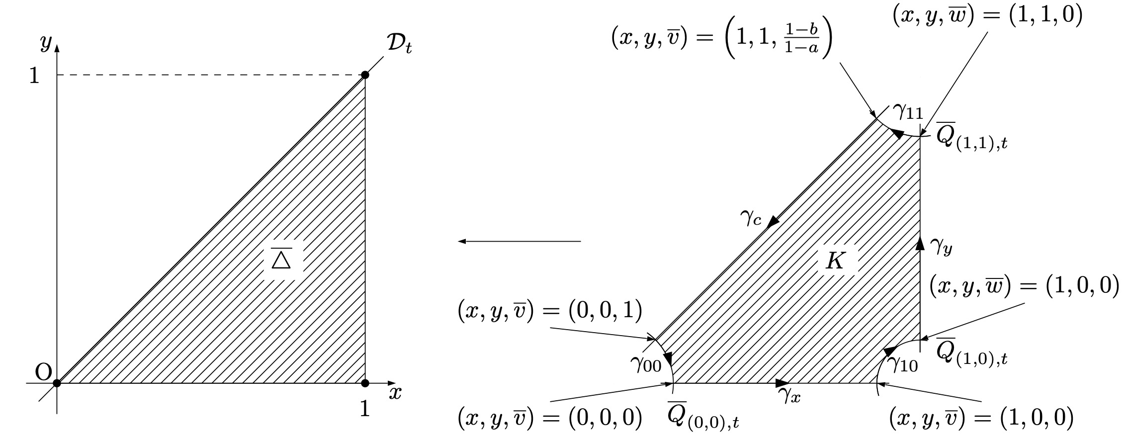
Figure 4. The figure of $K$ and paths on its boundary

Definition 8.6.

Since $\triangle\subset\overline{{\mathcal{X}}}_{t}^{\mathrm{an}}$ does not intersect with the branching locus of the double covering ${\mathcal{X}}_{t}^{\mathrm{an}}\rightarrow\overline{{\mathcal{X}}}_{t}^{\mathrm{an}}$, the inverse image of $\triangle$ by ${\mathcal{X}}_{t}^{\mathrm{an}}\rightarrow\overline{{\mathcal{X}}}_{t}^{\mathrm{an}}$ decomposes into the disjoint union of $\triangle_{+}$ and $\triangle_{-}$, which are both homeomorphic to $\triangle\subset\overline{{\mathcal{X}}}_{t}$ (Note that $\triangle$ is simply connected). We define $K_{+}$ and $K_{-}$ as the closure of $\triangle_{+}$ and $\triangle_{-}$. We choose $K_{+}$ and $K_{-}$ so that $K_{+}$ contains $(x,y,v)=(0,0,1)$ and $K_{-}$ contains $(x,y,v)=(0,0,-1)$.

(174)

By the condition (4)(5) in Definition 8.5, we can confirm that $K_{\pm}$ are $C^{\infty}$ manifolds with corners. Since $K_{\pm}$ are compact and have the natural orientation induced by $\triangle_{\pm}$, we can regard them as 2-chains on ${\mathcal{X}}_{t}^{\mathrm{an}}$.

We define paths $\gamma_{c,\pm},\gamma_{11,\pm},\gamma_{y},\gamma_{10,\pm},\gamma_{x}$ and $\gamma_{00,\pm}$ on ${\mathcal{X}}^{\mathrm{an}}_{t}$ appearing in the boundaries $\partial K_{+}$ and $\partial K_{-}$ as in Figure 5. They satisfy the following properties.

1. The path $\gamma_{c,+}$ (resp. $\gamma_{c,-}$) is the lift of $\gamma_{c}$ to $K_{+}$ (resp. $K_{-}$) and it is on the curve ${\mathcal{C}}_{t}^{\mathrm{an}}\subset{\mathcal{X}}_{t}^{\mathrm{an}}$. Note that by the condition (3) in Definition 8.5, its terminal point is $(x,y,v)=(0,0,1)$ (resp. $(x,y,v)=(0,0,-1)$) and its initial point is $(x,y,v)=\left(1,1,\frac{\sqrt{1-b}}{\sqrt{1-a}}\right)$ (resp. $(x,y,v)=\left(1,1,-\frac{\sqrt{1-b}}{\sqrt{1-a}}\right)$).

2. The paths $\gamma_{00,+},\gamma_{10,+}$ and $\gamma_{10,+}$ (resp. $\gamma_{00,-},\gamma_{10,-}$ and $\gamma_{10,-}$) are the lift of $\gamma_{00},\gamma_{10}$ and $\gamma_{11}$ to $K_{+}$ (resp. $K_{-}$) and they are on the exceptional curves $Q_{(0,0),t}^{\mathrm{an}},Q_{(1,0),t}^{\mathrm{an}}$ and $Q_{(1,1),t}^{\mathrm{an}}$ respectively.

3. Since $\gamma_{x}$ and $\gamma_{y}$ on $\overline{{\mathcal{X}}}_{t}^{\mathrm{an}}$ are contained in the branching locus of ${\mathcal{X}}^{\mathrm{an}}_{t}\rightarrow\overline{{\mathcal{X}}}^{\mathrm{an}}_{t}$, there exist unique lifts of them to ${\mathcal{X}}_{t}$. We denote their lifts by the same symbol $\gamma_{x}$ and $\gamma_{y}$.

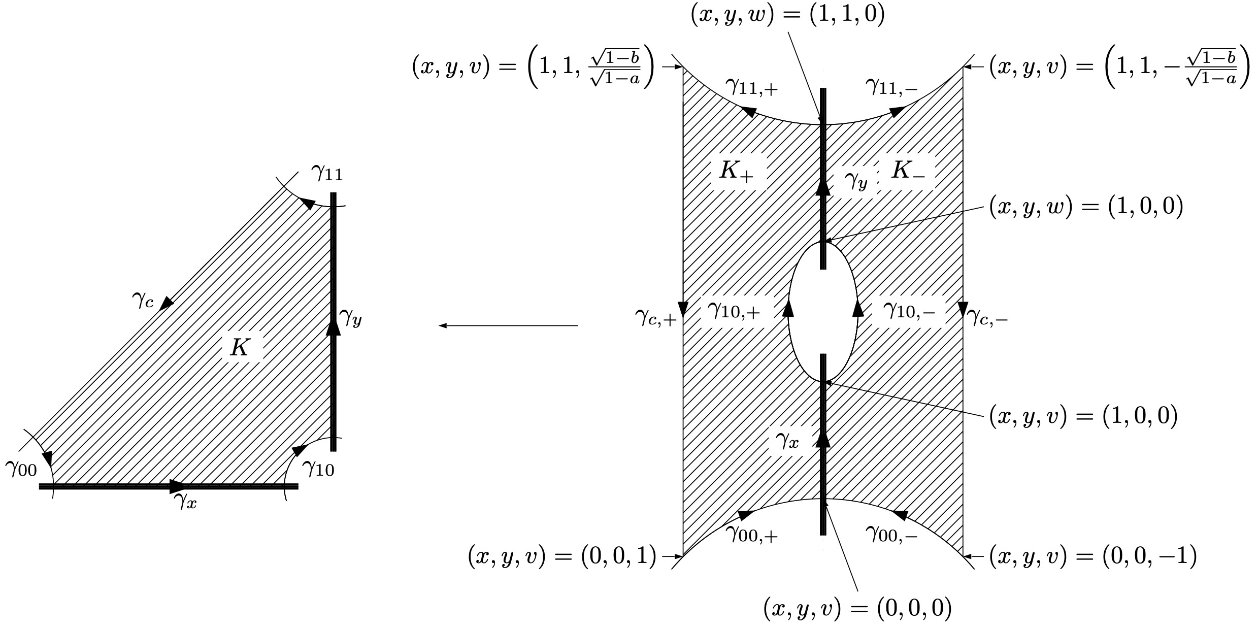
Figure 5. The figure of $K_{+},K_{-}$ and paths on their boundaries

Proposition 8.7.

The 2-chain $K_{+}-K_{-}\in S_{2}({\mathcal{X}}_{t}^{\mathrm{an}})$ is a 2-chain associated with $\xi_{1,t}-\xi_{0,t}$ in a weak sense.

We use the following lemma. The proof is immediate since $H_{1}(({\mathbb{P}}^{1}_{\mathbb{C}})^{\mathrm{an}})=0$.

Lemma 8.8.

If $\gamma,\gamma^{\prime}\in S_{1}(({\mathbb{P}}^{1}_{\mathbb{C}})^{\mathrm{an}})$ satisfy $\partial\gamma=\partial\gamma^{\prime}$, then $\gamma-\gamma^{\prime}\in B_{1}(({\mathbb{P}}^{1}_{\mathbb{C}})^{\mathrm{an}})$.

Proof.

(Proposition 8.7) By Proposition 5.10, $\xi_{1,t}-\xi_{0,t}$ is represented by the following element in $\bigoplus_{Z\in{\mathcal{X}}_{t}^{(1)}}R(Z)^{\times}$.

$$\left({\mathcal{C}}_{t},\frac{(v-1)\left(v+\frac{\sqrt{1-b}}{\sqrt{1-a}}\right)}{(v+1)\left(v-\frac{\sqrt{1-b}}{\sqrt{1-a}}\right)}\right)+\left(Q_{(0,0),t},\frac{v+1}{v-1}\right)+\left(Q_{(1,1),t},\frac{v-\frac{\sqrt{1-b}}{\sqrt{1-a}}}{v+\frac{\sqrt{1-b}}{\sqrt{1-a}}}\right)$$ (175)

By Figure 5, we see that that

$$\partial(\gamma_{c,+}-\gamma_{c,-})={\mathrm{div}}_{{\mathcal{C}}_{t}}\left(\frac{(v-1)\left(v+\frac{\sqrt{1-b}}{\sqrt{1-a}}\right)}{(v+1)\left(v-\frac{\sqrt{1-b}}{\sqrt{1-a}}\right)}\right),\quad\partial(\gamma_{10,+}-\gamma_{10,-})=0$$ (176)

$$\partial(\gamma_{00,+}-\gamma_{00,-})={\mathrm{div}}_{Q_{(0,0),t}}\left(\frac{v+1}{v-1}\right),\quad\partial(\gamma_{11,+}-\gamma_{11,-})={\mathrm{div}}_{Q_{(1,1),t}}\left(\frac{v-\frac{\sqrt{1-b}}{\sqrt{1-a}}}{v+\frac{\sqrt{1-b}}{\sqrt{1-a}}}\right)$$

Since ${\mathcal{C}}_{t},Q_{(0,0),t},Q_{(1,1),t}$ and $Q_{(1,0),t}$ are isomorphic to ${\mathbb{P}}^{1}_{\mathbb{C}}$, by Lemma 8.8, $(\gamma_{c,+}-\gamma_{c,-})+(\gamma_{11,+}-\gamma_{11,-})+(\gamma_{10,+}-\gamma_{10,-})+(\gamma_{00,+}-\gamma_{00,-})$ is a 1-cycle associated with $\xi_{1,t}-\xi_{0,t}$ in a weak sense. Since we have

$$\partial(K_{+}-K_{-})=(\gamma_{c,+}-\gamma_{c,-})+(\gamma_{11,+}-\gamma_{11,-})+(\gamma_{10,+}-\gamma_{10,-})+(\gamma_{00,+}-\gamma_{00,-}),$$ (177)

the result follows from Proposition 8.4. ∎

8.3. Calculation of the transcendental regulator map at $t\in T^{\circ}({\mathbb{C}})$

Since we have constructed a 2-chain associated with $\xi_{1,t}-\xi_{0,t}$, we can compute the image of $\xi_{1,t}-\xi_{0,t}$ under the transcendental regulator map by Proposition 8.4.

Definition 8.9.

Since ${\mathcal{X}}_{t}$ is a $K3$ surface and the holomorphic 2-form $\omega_{t}$ in Definition 7.1 is non-zero, the following map is an isomorphism between abelian groups.

(178)

We denote this map by ${\mathrm{ev}}_{t}$. Hereafter we concern periods of Kummer surfaces ${\mathcal{X}}_{t}$ for $t\in T^{\circ}({\mathbb{C}})$, we simply write ${\mathcal{P}}({\mathcal{X}}_{t},\omega_{t})$ as ${\mathcal{P}}_{\omega_{t}}$. Furthermore, the image of $x\in{\mathbb{C}}$ under the natural projection ${\mathbb{C}}\rightarrow{\mathbb{C}}/{\mathcal{P}}_{\omega_{t}}$ is denoted by $[x]\in{\mathbb{C}}/{\mathcal{P}}_{\omega_{t}}$.

Definition-Proposition 8.10.

Let $t\in T^{\circ}({\mathbb{C}})$. Choose a path $\gamma$ satisfying the conditions in Definition 8.5 at $t$. We can take an open neighborhood $U$ of $t$ in $(T^{\circ})^{\mathrm{an}}$ in the classical topology such that $\gamma$ satisfies the conditions in Definition 8.5 at every point on $U$. Then we have the following.

1. The following integral converges and defines a holomorphic function ${\mathcal{L}}$ on $U$.

   $${\mathcal{L}}(t)=\int_{\triangle}\frac{\gamma^{\prime}(p)\gamma^{\prime}(q)dpdq}{\sqrt{\gamma(p)(1-\gamma(p))(1-a\gamma(p))}\cdot\sqrt{\gamma(q)(1-\gamma(q))(1-b\gamma(q))}}\quad(t\in U)$$ (179)

   Note that since the branch of $\sqrt{z(1-z)(1-az)}$ and $\sqrt{z(1-z)(1-bz)}$ along $\gamma$ is fixed by Definition 8.5, the branch of the integrand on $\triangle$ is also fixed.

2. The image of $\xi_{1,t}-\xi_{0,t}$ under the transcendental regulator map $r$ is as follows.

   $${\mathrm{ev}}_{t}(r(\xi_{1,t}-\xi_{0,t}))=2[{\mathcal{L}}(t)]\quad\in{\mathbb{C}}/{\mathcal{P}}_{\omega_{t}}$$ (180)

3. If we choose a different path $\gamma$, we get another local holomorphic function ${\mathcal{L}}^{\prime}$. However, the difference ${\mathcal{L}}(t)-{\mathcal{L}}^{\prime}(t)\in{\mathbb{C}}$ should lie in $\frac{1}{2}{\mathcal{P}}_{\omega_{t}}$.

Proof.

By the construction of $\Delta_{+}\subset{\mathcal{X}}_{t}^{\mathrm{an}}$, we see that $\Delta_{+}$ coincides with the image of the following map.

(181)

Hence the right hand side of (179) coincides with $\int_{\Delta_{+}}\omega_{t}$. Since the integrand is $C^{\infty}$ on the boundary of $\Delta_{+}$, we have $\int_{\Delta_{+}}\omega_{t}=\int_{K_{+}}\omega_{t}$. Thus the right hand side of (179) can be regarded as integration of a $C^{\infty}$-function on a compact $C^{\infty}$-manifold with corners. Furthermore, the integrand is holomorphic with respect to $a,b$, which are local coordinates of $(T^{\circ})^{\mathrm{an}}$. Hence we have (1). By Proposition 8.4 and Proposition 8.7, we have

$${\mathrm{ev}}_{t}(r(\xi_{1,t}-\xi_{0,t}))=\int_{K_{+}}\omega_{t}-\int_{K_{-}}\omega_{t}\in{\mathbb{C}}/{\mathcal{P}}_{\omega_{t}}$$ (182)

Since $\int_{K_{+}}\omega_{t}=-\int_{K_{-}}\omega_{t}={\mathcal{L}}(t)$ by definition, we have (2). Then by (2), $2[{\mathcal{L}}(t)]$ is determined up to elements in ${\mathcal{P}}_{\omega_{t}}$. Thus we have (3). ∎

At last, we calculate the image of ${\mathcal{L}}$ under the Picard-Fuchs operator ${\mathscr{D}}$ in Definition 7.8. This calculation is used in the rank estimation of the image of $\Xi_{t}$ under the transcendental regulator map in Section 9. This theorem also gives a system of differential equations which ${\mathcal{L}}$ satisfies.

Theorem 8.11.

Let ${\mathcal{L}}$ be the local holomorphic function defined in Definition 8.10. Then we have

$${\mathscr{D}}({\mathcal{L}})=\frac{1}{a-b}\cdot\begin{pmatrix}\frac{\sqrt{1-b}}{\sqrt{1-a}}-1\\[6.45831pt] 1-\frac{\sqrt{1-a}}{\sqrt{1-b}}\end{pmatrix}$$ (183)

Proof.

A local holomorphic function $H(c,z)=-\frac{\sqrt{z(1-z)}}{2(1-cz)^{\frac{3}{2}}}$ satisfies

$$L_{c}\left(\frac{1}{\sqrt{z(1-z)(1-cz)}}\right)=\frac{\partial H(c,z)}{\partial z}.$$ (184)

where $L_{c}$ is the differential operator defined in Definition 7.4. Then we have the following equation on 2-forms on ${\mathcal{X}}_{t}$.

$${\mathscr{D}}_{1}\left(\frac{1}{\sqrt{x(1-x)(1-ax)}\cdot\sqrt{y(1-y)(1-by)}}\right)dx\wedge dy=d\left(\frac{H(a,x)dy}{\sqrt{y(1-y)(1-by)}}\right)$$ (185)

This equation holds on an open neighborhood of $K_{+}$. By the definition of ${\mathcal{L}}$ and Stokes theorem on ${\mathcal{X}}_{t}$, we have the following.

$${\mathscr{D}}_{1}({\mathcal{L}})={\mathscr{D}}_{1}\left(\int_{K_{+}}\frac{\gamma^{\prime}(p)\gamma^{\prime}(q)dpdq}{\sqrt{\gamma(p)(1-\gamma(p))(1-a\gamma(p))}\cdot\sqrt{\gamma(q)(1-\gamma(q))(1-b\gamma(q))}}\right)$$ (186)

$$=\int_{K_{+}}d\left(\frac{H(a,\gamma(p))\gamma^{\prime}(q)dq}{\sqrt{\gamma(q)(1-\gamma(q))(1-b\gamma(q))}}\right)=\int_{\partial K_{+}}\frac{H(a,\gamma(p))\gamma^{\prime}(q)dq}{\sqrt{\gamma(q)(1-\gamma(q))(1-b\gamma(q))}}$$

Since the 1-form $\frac{H(a,x)dy}{\sqrt{y(1-y)(1-by)}}$ vanishes at $\{y=0\}$ and $\{x=1\}$, we have

$${\mathscr{D}}_{1}({\mathcal{L}})=\frac{1}{2}\int_{0}^{1}\frac{dz}{(1-bz)^{\frac{1}{2}}(1-az)^{\frac{3}{2}}}=\frac{1}{a-b}\int_{1}^{\frac{\sqrt{1-b}}{\sqrt{1-a}}}du=\frac{1}{a-b}\cdot\left(\frac{\sqrt{1-b}}{\sqrt{1-a}}-1\right).$$ (187)

Here we use the coordinate transform $u=\frac{\sqrt{1-bz}}{\sqrt{1-az}}$. We can compute ${\mathscr{D}}_{2}({\mathcal{L}})$ similarly. ∎

9. Estimation of the rank of the image of $\Xi$ under the transcendental regulator maps

In this section, we prove Theorem 1.1. The outline of the proof is as follows.

1. We construct a ${\mathbb{Q}}$-linear sheaf ${\mathcal{Q}}_{\omega}$ on $(T^{\prime})^{\mathrm{an}}$ as a quotient of the sheaf of holomorphic functions ${\mathcal{O}}_{(T^{\prime})^{\mathrm{an}}}$ by a locally constant subsheaf ${\mathcal{P}}_{\omega}$ generated by period functions $P_{ij}$. For each $t\in(T^{\prime})^{\mathrm{an}}$, we have a “evaluation” map ${\mathcal{Q}}_{\omega}(T^{\prime})\rightarrow{\mathbb{C}}/{\mathbb{Q}}{\mathcal{P}}_{\omega_{t}}\simeq H^{2,0}({\mathcal{X}}_{t}^{\mathrm{an}})^{\vee}/H_{2}({\mathcal{X}}_{t},{\mathbb{Q}})$. We see that the Picard-Fuchs differential operator ${\mathscr{D}}$ factors through the sheaf ${\mathcal{Q}}_{\omega}$ (Definition 9.13).

2. The ${\mathbb{Q}}$-linear space ${\mathcal{Q}}_{\omega}(T^{\circ})$ is the target of a “relative transcendental regulator map” $R_{\omega}:\Xi\rightarrow{\mathcal{Q}}_{\omega}(T^{\circ})$ (Definition 9.11). The “value” of $R_{\omega}(\xi)$ at $t\in T^{\circ}({\mathbb{C}})$ coincides with $r(\xi_{t})$ modulo torsion.

3. By the formula of the $\widetilde{G}$-action on $\omega_{t}$ in Proposition 7.2, we have the following commutative diagram (Proposition 9.6).

   (188)

4. By the diagram above, we can define a $\widetilde{G}$-action $\{\Upsilon_{\widetilde{\rho}}\}_{\widetilde{\rho}\in\widetilde{G}}$ on ${\mathcal{Q}}_{\omega}$ (Definition 9.7) so that the relative transcendental regulator map $R_{\omega}$ is equivariant to $\widetilde{G}$-actions (Proposition 9.11). Furthermore, we can also define a $\widetilde{G}$-action $\{\Theta_{\widetilde{\rho}}\}_{\widetilde{\rho}\in\widetilde{G}}$ on ${\mathcal{O}}_{(T^{\prime})^{\mathrm{an}}}^{\oplus 2}$ (Definition 9.14) so that the Picard-Fuchs differential operator ${\mathscr{D}}$ is equivariant to $\widetilde{G}$-actions (Proposition 9.15).

5. In conclusion, we have the following diagram for $\widetilde{\rho}\in\widetilde{G}$.

   (189)

   By this diagram, we can compute the image ${\mathscr{D}}\circ R_{\omega}(\Xi)$ (Table 8) and get the desired rank estimate (Theorem 9.20).

9.1. The definition of the sheaves ${\mathcal{P}}_{\omega}$ and ${\mathcal{Q}}_{\omega}$

In this section, we define the sheaves ${\mathcal{P}}_{\omega}$ and ${\mathcal{Q}}_{\omega}$ and prove their properties.

Definition 9.1.

We regard the sheaf ${\mathcal{O}}_{(T^{\prime})^{\mathrm{an}}}$ of holomorphic functions on $(T^{\prime})^{\mathrm{an}}$ as a ${\mathbb{Q}}$-linear sheaf. We define a subsheaf ${\mathcal{P}}_{\omega}\subset{\mathcal{O}}_{(T^{\prime})^{\mathrm{an}}}$ as the unique sheaf satisfying the following property:

$$\text{For any open set }U\subset(T^{\prime})^{\mathrm{an}}\text{ in the classical topology such that }P_{ij}\text{ are defined, }$$ (190)

$${\mathcal{P}}_{\omega}|_{U}\text{ is the subsheaf generated (as a ${\mathbb{Q}}$-linear sheaf) by }P_{ij}\text{ for }i,j\in\{1,2\}.$$

where $P_{ij}$ are the local holomorphic functions defined in Definition 7.7. Then we define a sheaf ${\mathcal{Q}}_{\omega}$ as the quotient sheaf ${\mathcal{O}}_{(T^{\prime})^{\mathrm{an}}}/{\mathcal{P}}_{\omega}$. For a local section $f$ of ${\mathcal{O}}_{(T^{\prime})^{\mathrm{an}}}$, $[f]$ denotes the image of $f$ under the quotient map ${\mathcal{O}}_{(T^{\prime})^{\mathrm{an}}}\rightarrow{\mathcal{Q}}_{\omega}$.

The existence of ${\mathcal{P}}_{\omega}$ can be confirmed by the following remark.

Remark 9.2.

Let $\pi:{\mathcal{X}}^{\prime}\rightarrow T^{\prime}$ be the structure morphism. We define the following sheaves ${\mathcal{P}},{\mathcal{Q}}$ on $(T^{\prime})^{\mathrm{an}}$.

$${\mathcal{P}}=\mathrm{Im}(R^{2}\pi_{*}\underline{{\mathbb{Q}}}_{({\mathcal{X}}^{\prime})^{\mathrm{an}}}\rightarrow\mathcal{H}om_{{\mathcal{O}}_{(T^{\prime})^{\mathrm{an}}}}(\pi_{*}\Omega^{2}_{{\mathcal{X}}^{\prime}/T^{\prime}},{\mathcal{O}}_{(T^{\prime})^{\mathrm{an}}}))$$ (191)

$${\mathcal{Q}}=\mathrm{Coker}(R^{2}\pi_{*}\underline{{\mathbb{Q}}}_{({\mathcal{X}}^{\prime})^{\mathrm{an}}}\rightarrow\mathcal{H}om_{{\mathcal{O}}_{(T^{\prime})^{\mathrm{an}}}}(\pi_{*}\Omega^{2}_{{\mathcal{X}}^{\prime}/T^{\prime}},{\mathcal{O}}_{(T^{\prime})^{\mathrm{an}}}))$$

where $\underline{{\mathbb{Q}}}_{({\mathcal{X}}^{\prime})^{\mathrm{an}}}$ is the constant sheaf with coefficients in ${\mathbb{Q}}$ on $({\mathcal{X}}^{\prime})^{\mathrm{an}}$ and the morphism $R^{2}\pi_{*}\underline{{\mathbb{Q}}}_{({\mathcal{X}}^{\prime})^{\mathrm{an}}}\rightarrow\mathcal{H}om_{{\mathcal{O}}_{(T^{\prime})^{\mathrm{an}}}}(\pi_{*}\Omega^{2}_{{\mathcal{X}}^{\prime}/T^{\prime}},{\mathcal{O}}_{(T^{\prime})^{\mathrm{an}}})$ is induced by the fiber integration.

Since ${\mathcal{X}}^{\prime}$ is a family of $K3$ surface, $\pi_{*}\Omega^{2}_{{\mathcal{X}}^{\prime}/T^{\prime}}$ is a locally free ${\mathcal{O}}_{(T^{\prime})^{\mathrm{an}}}$-module of rank 1. Then we have an isomorphism ${\mathcal{O}}_{(T^{\prime})^{\mathrm{an}}}\simeq\mathcal{H}om_{{\mathcal{O}}_{(T^{\prime})^{\mathrm{an}}}}(\pi_{*}\Omega^{2}_{{\mathcal{X}}^{\prime}/T^{\prime}},{\mathcal{O}}_{(T^{\prime})^{\mathrm{an}}})$ induced by $\varphi\mapsto\varphi\cdot\omega$ where $\omega$ is the 2-form in Definition 7.1. Under this isomorphism, we have ${\mathcal{P}}\simeq{\mathcal{P}}_{\omega}$ and ${\mathcal{Q}}\simeq{\mathcal{Q}}_{\omega}$. Since $\pi:{\mathcal{X}}^{\prime}\rightarrow T^{\prime}$ is a topologically locally trivial fibration, for a sufficiently small open neighborhood in the classical topology, we have a ${\mathbb{Q}}$-basis in ${\mathcal{P}}|_{U}$. The holomorphic functions $P_{ij}\>(i,j\in\{1,2\})$ are the images of such a basis under ${\mathcal{P}}|_{U}\simeq{\mathcal{P}}_{\omega}|_{U}$.

Definition 9.3.

For each $t\in T^{\prime}({\mathbb{C}})$, ${\mathcal{O}}_{(T^{\prime})^{\mathrm{an}},t}$ denotes the stalk of ${\mathcal{O}}_{(T^{\prime})^{\mathrm{an}}}$ at $t$. We define the evaluation map $m_{t}$ by

(192)

For an open neighborhood $U$ of $t$ in the classical topology, composition of $m_{t}$ and a restriction map ${\mathcal{O}}_{(T^{\prime})^{\mathrm{an}}}(U)\rightarrow{\mathcal{O}}_{(T^{\prime})^{\mathrm{an}},t}$ is also denoted by $m_{t}$. Furthermore, since ${\mathcal{P}}_{\omega_{t}}\subset{\mathbb{C}}$ is generated by the values of $P_{ij}$ at $t$ by Definition 7.7, $m_{t}:{\mathcal{O}}_{(T^{\prime})^{\mathrm{an}},t}\rightarrow{\mathbb{C}}$ induces the following map ${\mathcal{Q}}_{\omega,t}\rightarrow{\mathbb{C}}/{\mathbb{Q}}{\mathcal{P}}_{\omega_{t}}$.

(193)

where ${\mathbb{Q}}{\mathcal{P}}_{\omega_{t}}\subset{\mathbb{C}}$ is a ${\mathbb{Q}}$-linear subspace of ${\mathbb{C}}$ generated by ${\mathcal{P}}_{\omega_{t}}$. We also denote this map by $m_{t}$. Furthermore, the composite of $m_{t}$ and the restriction map of ${\mathcal{Q}}_{\omega}$ is also denoted by $m_{t}$.

Proposition 9.4.

Let $U$ be an open subset of $(T^{\prime})^{\mathrm{an}}$ in the classical topology and $\varphi\in{\mathcal{O}}_{(T^{\prime})^{\mathrm{an}}}(U)$. Then $\varphi(t)\not\in{\mathbb{Q}}{\mathcal{P}}_{\omega_{t}}$ for very general $t\in U$ if and only if $\varphi\not\in{\mathcal{P}}_{\omega}(U)$. Especially, if $\varphi\in{\mathcal{O}}_{(T^{\prime})^{\mathrm{an}}}(U)$ satisfies that $\varphi(t)\in{\mathbb{Q}}{\mathcal{P}}_{\omega_{t}}$ holds for every $t\in U$, then $\varphi$ is a section of ${\mathcal{P}}_{\omega}(U)$.

Proof.

We will prove the former part of the proposition. We may assume $U$ is so small that $P_{ij}$ are defined on $U$. For each quadruple $\underline{c}=(c_{ij})\in{\mathbb{Q}}^{\oplus 4}$, we define a holomorphic function $F_{\underline{c}}$ by

$$F_{\underline{c}}=\varphi-\sum_{i,j}c_{ij}P_{ij}.$$ (194)

Consider the countable family $\{F_{\underline{c}}\}_{\underline{c}\in{\mathbb{Q}}^{4}}$ of holomorphic functions on $U$. If $\varphi\not\in{\mathcal{P}}_{\omega}(U)$, they are non-zero holomorphic functions. Especially, for very general $t\in U$, $F_{\underline{c}}(t)\neq 0$ holds for all $\underline{c}\in{\mathbb{Q}}^{4}$. Since ${\mathcal{P}}_{\omega_{t}}$ is generated (as a ${\mathbb{Q}}$-linear subspace of ${\mathbb{C}}$) by $P_{ij}(t)$, we see that $F_{\underline{c}}(t)\neq 0$ holds for all $\underline{c}\in{\mathbb{Q}}^{4}$ is equivalent to $\varphi(t)\not\in{\mathbb{Q}}{\mathcal{P}}_{\omega_{t}}$. Converse is clear. The latter part follows from the former part. ∎

The sheaf ${\mathcal{Q}}_{\omega}$ has the following property. This lemma enables us to reduce the computation of ${\mathcal{Q}}_{\omega}$ to that of its restriction at each point on $U$.

Lemma 9.5.

For each open subset $U$ of $(T^{\prime})^{\mathrm{an}}$ in the classical topology and non-zero section $x\in{\mathcal{Q}}_{\omega}(U)$, the restriction $m_{t}(x)$ is non-zero for very general $t\in U$. Especially, the following map is injective.

(195)

Proof.

We can shrink $U$ so small that $x$ is of the form $x=[\varphi]$ for $\varphi\in{\mathcal{O}}_{(T^{\prime})^{\mathrm{an}}}(U)$. Then the results follows from Proposition 9.4. ∎

9.2. A $\widetilde{G}$-action on ${\mathcal{Q}}_{\omega}$

First, we see that how $\widetilde{G}$ acts on ${\mathbb{C}}/{\mathcal{P}}_{\omega_{t}}$.

Proposition 9.6.

Let $t\in T^{\circ}({\mathbb{C}})$ and $\widetilde{\rho}=(\rho,\zeta)\in\widetilde{G}$. Let $\widetilde{\rho}_{t}:{\mathcal{X}}_{t}\xrightarrow{\>\sim\>}{\mathcal{X}}_{\underline{\rho}(t)}$ be the automorphism defined in Definition 4.23.

1. We have ${\mathcal{P}}_{\omega_{\underline{\rho}(t)}}=\widetilde{\chi}(\widetilde{\rho})(t)\cdot{\mathcal{P}}_{\omega_{t}}$ as a subgroup of ${\mathbb{C}}$. Here $\widetilde{\chi}(\widetilde{\rho})(t)\in{\mathbb{C}}$ is the value of $\widetilde{\chi}(\widetilde{\rho})\in B^{\prime}$ in Defintion 4.18 at $t$.

2. From (1), the following map is well-defined.

   (196)

3. We have the following commutative diagram.

   (197)

   where the right vertical map is $(\ref{chimul})$ above.

Proof.

Note that the following equation holds for every 2-chain $\Gamma\in S_{2}({\mathcal{X}}_{t}^{\mathrm{an}})$.

$$\int_{(\widetilde{\rho}_{t})_{*}\Gamma}\omega_{\underline{\rho}(t)}=\int_{\Gamma}(\widetilde{\rho}_{t})^{*}\omega_{\underline{\rho}(t)}=\widetilde{\chi}(\widetilde{\rho})(t)\cdot\int_{\Gamma}\omega_{t}$$ (198)

For the second equality, we use Proposition 7.2. By the equations (198) for $\Gamma\in Z_{2}({\mathcal{X}}_{t}^{\mathrm{an}})$, we can show (1). If $\Gamma$ is a 2-chain associated with $\xi\in{\mathrm{CH}}^{2}({\mathcal{X}}_{t},1)$, then $(\widetilde{\rho}_{t})_{*}\Gamma$ is a 2-chain associated with $(\widetilde{\rho}_{t})_{*}\xi\in{\mathrm{CH}}^{2}({\mathcal{X}}_{\underline{\rho}(t)},1)$. Hence by the equation (198) for a 2-chain $\Gamma$ associated with $\xi$, we see that the whole rectangle in (197) commutes. Since ${\mathrm{ev}}_{t},{\mathrm{ev}}_{\underline{\rho}(t)}$ are isomorphisms by Definition 8.9, all squares in (197) commute. ∎

Then we will define a $\widetilde{G}$-linearization on ${\mathcal{O}}_{(T^{\prime})^{\mathrm{an}}}$.

Definition 9.7.

Let $\widetilde{\rho}=(\rho,\zeta)\in\widetilde{G}$. We define a morphism $\Upsilon_{\widetilde{\rho}}:{\mathcal{O}}_{(T^{\prime})^{\mathrm{an}}}\rightarrow(\underline{\rho}^{-1})_{*}{\mathcal{O}}_{(T^{\prime})^{\mathrm{an}}}$ as follows. Let $U$ be an open subset of $(T^{\prime})^{\mathrm{an}}$ in the classical topology.

(199)

Then $\{\Upsilon_{\widetilde{\rho}}\}_{\widetilde{\rho}\in\widetilde{G}}$ satisfies the cocycle condition. In other words, the following diagram commutes for $\widetilde{\rho},\widetilde{\rho}^{\prime}\in\widetilde{G}$.

(200)

Proposition 9.8.

For $\widetilde{\rho}\in\widetilde{G}$ and an open subset $U\subset(T^{\prime})^{\mathrm{an}}$ in the classical topology, we have

$$\Upsilon_{\widetilde{\rho}}({\mathcal{P}}_{\omega}(U))={\mathcal{P}}_{\omega}(\underline{\rho}(U)).$$ (201)

Proof.

It is enough to show only $(\subset)$ by the cocycle condition. Let $\varphi\in{\mathcal{P}}_{\omega}(U)$. Then for $\underline{\rho}(t)\in\underline{\rho}(T)$, we have

$$m_{\underline{\rho}(t)}(\Upsilon_{\widetilde{\rho}}(\varphi)) =m_{\underline{\rho}(t)}((\underline{\rho}^{-1})^{\sharp}(\widetilde{\chi}(\widetilde{\rho})\cdot\varphi))=m_{t}(\widetilde{\chi}(\widetilde{\rho})\cdot\varphi)$$ (202)

$$=\widetilde{\chi}(\widetilde{\rho})(t)\cdot\varphi(t)\in\widetilde{\chi}(\widetilde{\rho})(t)\cdot{\mathbb{Q}}{\mathcal{P}}_{\omega_{t}}={\mathbb{Q}}{\mathcal{P}}_{\omega_{\underline{\rho}(t)}}.$$

The last equality follows from Proposition 9.6. By Proposition 9.4, $\Upsilon_{\widetilde{\rho}}(\varphi)\in{\mathcal{P}}_{\omega}(\underline{\rho}(U))$. ∎

By the proposition above, the $\widetilde{G}$-linearization on ${\mathcal{O}}_{(T^{\prime})^{\mathrm{an}}}$ induces a $\widetilde{G}$-linearization on ${\mathcal{Q}}_{\omega}$.

Definition 9.9.

By Proposition 9.8, $\Upsilon_{\widetilde{\rho}}:{\mathcal{O}}_{(T^{\prime})^{\mathrm{an}}}\rightarrow(\underline{\rho}^{-1})_{*}{\mathcal{O}}_{(T^{\prime})^{\mathrm{an}}}$ induces a morphism ${\mathcal{Q}}_{\omega}\rightarrow(\underline{\rho}^{-1})_{*}{\mathcal{Q}}_{\omega}$. Since $\underline{\rho}(T^{\circ})=T^{\circ}$, we have the following ${\mathbb{Q}}$-linear map.

(203)

By the cocycle condition (200), $\Upsilon_{\widetilde{\rho}}$ defines a $\widetilde{G}$-action on the ${\mathbb{Q}}$-linear space ${\mathcal{Q}}_{\omega}(T^{\circ})$. By Definition 9.7, the following diagram commutes for $t\in(T^{\circ})^{\mathrm{an}}$.

(204)

where the right vertical map is induced by (2) of Proposition 9.6.

9.3. Construction of the relative transcendental regulator map $R_{\omega}$

In this section, we construct the relative transcendental regulator map and show the $\widetilde{G}$-equivariance of $R_{\omega}$. First, we construct an element in ${\mathcal{Q}}_{\omega}(T^{\circ})$ corresponding to a half of the image of $\xi_{1}-\xi_{0}$ under the relative transcendental regulator map.

Proposition 9.10.

There exists a unique element $[{\mathcal{L}}]\in{\mathcal{Q}}_{\omega}(T^{\circ})$ such that for $t\in T^{\circ}({\mathbb{C}})$,

$$m_{t}([{\mathcal{L}}])=[{\mathcal{L}}(t)]$$ (205)

where ${\mathcal{L}}(t)\in{\mathbb{C}}$ denotes the value of the local holomorphic function ${\mathcal{L}}$ in Definition 8.10.

Proof.

The uniqueness follows from Lemma 9.5. We show the existence. We take an open cover $\{U_{i}\}_{i\in I}$ of $(T^{\circ})^{\mathrm{an}}$ such that ${\mathcal{L}}$ is defined on each $U_{i}$. Let ${\mathcal{L}}_{i}\in{\mathcal{O}}_{(T^{\prime})^{\mathrm{an}}}(U_{i})$ denote a holomorphic function ${\mathcal{L}}$ on $U_{i}$. It is enough to glue $[{\mathcal{L}}_{i}]\in{\mathcal{Q}}_{\omega}(U_{i})$. By Proposition 8.10, for each $t\in U_{i}\cap U_{j}$, ${\mathcal{L}}_{i}(t)-{\mathcal{L}}_{j}(t)\in{\mathbb{Q}}{\mathcal{P}}_{\omega_{t}}$. Then we have ${\mathcal{L}}_{i}-{\mathcal{L}}_{j}\in{\mathcal{P}}_{\omega}(U_{i}\cap U_{j})$ by Proposition 9.4. Hence we have $[{\mathcal{L}}_{i}]|_{U_{i}\cap U_{j}}=[{\mathcal{L}}_{j}]|_{U_{i}\cap U_{j}}$ in ${\mathcal{Q}}_{\omega}(U_{i}\cap U_{j})$ and we can check the gluing condition. ∎

Definition-Proposition 9.11.

$($Definition of $R_{\omega})$ There exists a unique group homomorphism

(206)

which satisfies the following properties. The map $R_{\omega}$ is called the relative transcendental regulator map.

1. For $t\in T^{\circ}({\mathbb{C}})$, the following diagram commutes.

   (207)

   where $i_{t}^{*}$ is the pull-back map in Definition 5.9, $r$ is the transcendental regulator map in Definition 8.2, ${\mathrm{ev}}_{t}$ is the map defined in Definition 8.9, $m_{t}$ is the map defined in Definition 9.3 and ${\mathbb{C}}/{\mathcal{P}}_{\omega_{t}}\rightarrow{\mathbb{C}}/{\mathbb{Q}}{\mathcal{P}}_{\omega_{t}}$ is the natural projection.

2. For $\widetilde{\rho}\in\widetilde{G}$, the following diagram commutes.

   (208)

Proof.

We will prove that there exists a unique map $R_{\omega}$ satisfying the condition (1) and $R_{\omega}$ satisfies (2).

The uniqueness follows from Lemma 9.5. If we define $R_{\omega}(\xi_{1}-\xi_{0})=2[{\mathcal{L}}]$ where $[{\mathcal{L}}]$ is the element defined in Proposition 9.10, we can check the commutativity of (207) for $\xi_{1}-\xi_{0}\in\Xi$ by Proposition 8.10. We can also define $R_{\omega}(\xi)$ for each $\xi\in\Xi$ so as to make the diagram (207) commute as follows: By Proposition 5.13, $\xi$ is represented by a product of $(\widetilde{\rho}^{-1})^{\sharp}(\psi_{\bullet})$ and $(\widetilde{\rho}^{-1})^{\sharp}(\varphi_{\bullet})$. They are on smooth families of curves over $T^{\circ}$ and their zeros and poles are also smooth over $T^{\circ}$. Hence by the similar method in Section 8, we see that ${\mathrm{ev}}_{t}(r(\xi))$ is represented by the value of the local holomorphic function as in Proposition 8.10. Hence by the similar argument in Proposition 9.10, we can define $R_{\omega}(\xi)\in{\mathcal{Q}}_{\omega}(T^{\circ})$. Hence we can check the existence of the map $R_{\omega}$ satisfying the condition (1).

Next, we will prove that $R_{\omega}$ satisfies (2). Consider the following diagram.

(209)

The left side face commutes by the associativity of pull-back maps on higher Chow groups ([Lev98] PartI, Chapter II, 2.1.6). The bottom face commutes by Proposition 9.6 and the right side face commutes by (204) in Definition 9.9. Since the front and back faces commute by (1), by Lemma 9.5, we see that the upper face commutes. ∎

By $\widetilde{G}$-equivariance of $R_{\omega}$, we have a $\widetilde{G}$-action on $R_{\omega}(\Xi)$. Then we have the upper estimate for ${\mathrm{rank}\>}R_{\omega}(\Xi)$. The proof below is simplified by advice from T. Saito.

Proposition 9.12.

We have the following.

1. For $\widetilde{\rho}\in\widetilde{G}_{\mathrm{fib}}$, we have $R_{\omega}(\widetilde{\rho}_{*}\Xi^{\mathrm{can}})=R_{\omega}(\Xi^{\mathrm{can}})$.

2. We have ${\mathrm{rank}\>}R_{\omega}(\Xi)\leq 18$.

3. For each $t\in T^{\circ}({\mathbb{C}})$, ${\mathrm{rank}\>}r(\Xi_{t})\leq 18$.

Proof.

By $\widetilde{G}$-equivariance of $R_{\omega}$, we have $R_{\omega}(\widetilde{\rho}_{*}\Xi^{\mathrm{can}})=\Upsilon_{\widetilde{\rho}}(R_{\omega}(\Xi^{\mathrm{can}}))$. For $\widetilde{\rho}\in\widetilde{G}_{\mathrm{fib}}$, we have $\Upsilon_{\widetilde{\rho}}=\pm 1$ by definition of $\Upsilon_{\widetilde{\rho}}$. Hence we have (1).

By (1) and Proposition 6.8, $R_{\omega}(\Xi^{\mathrm{can}})\subset R_{\omega}(\Xi)$ is stabilized under the $\widetilde{G}_{\mathrm{fib}}\widetilde{I}$-action. Especially, we have a $\widetilde{G}_{\mathrm{fib}}\widetilde{I}$-representation on $R_{\omega}(\Xi^{\mathrm{can}})$. Then the following $\widetilde{G}$-equivariant map is induced.

$$\mathrm{Ind}_{\widetilde{G}_{\mathrm{fib}}\widetilde{I}}^{\widetilde{G}}R_{\omega}(\Xi^{\mathrm{can}})\>{\longrightarrow}\>R_{\omega}(\Xi)$$ (210)

where $\mathrm{Ind}_{\widetilde{G}_{\mathrm{fib}}\widetilde{I}}^{\widetilde{G}}R_{\omega}(\Xi^{\mathrm{can}})$ denotes the induced representation. Since $R_{\omega}(\Xi)$ is the sum of $R_{\omega}(\widetilde{\rho}_{*}\Xi^{\mathrm{can}})$ for $\widetilde{\rho}\in\widetilde{G}$, the map (210) is surjective. Then we have

$${\mathrm{rank}\>}R_{\omega}(\Xi)\leq{\mathrm{rank}\>}\mathrm{Ind}_{\widetilde{G}_{\mathrm{fib}}\widetilde{I}}^{\widetilde{G}}R_{\omega}(\Xi^{\mathrm{can}})=|\widetilde{G}/\widetilde{G}_{\mathrm{fib}}\widetilde{I}|\cdot{\mathrm{rank}\>}R_{\omega}(\Xi^{\mathrm{can}})\leq 6\cdot 3.$$ (211)

Here we use $|\widetilde{G}/\widetilde{G}_{\mathrm{fib}}\widetilde{I}|=6$ by Proposition 6.12. Hence we have (2). By (2) and the commutative diagram (207), we have (3). ∎

9.4. The differential operator ${\mathscr{D}}$ and $\widetilde{G}$-actions

In this subsection, we define a $\widetilde{G}$-action on ${\mathcal{O}}_{(T^{\prime})^{\mathrm{an}}}^{\oplus 2}$ so that ${\mathscr{D}}$ is $\widetilde{G}$-equivariant. For this purpose, we prove transformation formulae of ${\mathscr{D}}$.

Definition 9.13.

Since the local holomorphic functions $P_{ij}$ are annihilated by the differential operator ${\mathscr{D}}:{\mathcal{O}}_{(T^{\prime})^{\mathrm{an}}}\rightarrow{\mathcal{O}}_{(T^{\prime})^{\mathrm{an}}}^{\oplus 2}$ in Definition 7.8, ${\mathcal{P}}_{\omega}\hookrightarrow{\mathcal{O}}_{(T^{\prime})^{\mathrm{an}}}\xrightarrow{{\mathscr{D}}}{\mathcal{O}}_{(T^{\prime})^{\mathrm{an}}}^{\oplus 2}$ is the 0-map. Hence the following morphism is induced. This morphism is also denoted by ${\mathscr{D}}$.

(212)

Definition 9.14.

Let $\widetilde{\rho}=(\rho,\zeta)\in\widetilde{G}$. Let $U$ be an open subset of $(T^{\prime})^{\mathrm{an}}$ in the classical topology. We define a morphism $\Theta_{\widetilde{\rho}}:{\mathcal{O}}_{(T^{\prime{\mathrm{an}}})}^{\oplus 2}\rightarrow(\underline{\rho}^{-1})_{*}{\mathcal{O}}_{(T^{\prime{\mathrm{an}}})}^{\oplus 2}$ as the following map.

(213)

Here $\chi^{(1)}$ and $\chi^{(2)}$ are the opposite 1-cocycles defined in Definition 4.16. Then $\{\Upsilon_{\widetilde{\rho}}\}_{\rho\in\widetilde{G}}$ satisfies the following cocycle condition for $\widetilde{\rho},\widetilde{\rho}^{\prime}\in\widetilde{G}$.

(214)

By the cocycle condition, $\Theta_{\widetilde{\rho}}:{\mathcal{O}}_{(T^{\prime})^{\mathrm{an}}}(T^{\circ})^{\oplus 2}\rightarrow{\mathcal{O}}_{(T^{\prime})^{\mathrm{an}}}(T^{\circ})^{\oplus 2}$ defines a $\widetilde{G}$-action on ${\mathcal{O}}_{(T^{\prime})^{\mathrm{an}}}(T^{\circ})^{\oplus 2}$.

The main purpose of this subsection is to prove the following.

Proposition 9.15.

For $\rho\in\widetilde{G}$, the following diagram commutes.

(215)

We need some preparation for proving Proposition 9.15. First, we define some differential operators twisted by $\underline{G}$-action.

Definition 9.16.

For $\underline{\rho}\in\underline{G}$, we define differential operators ${\mathscr{D}}_{i}^{\underline{\rho}}$ for $i=1,2$ as follows.

$${\mathscr{D}}^{\underline{\rho}}_{1}=a^{\prime}(1-a^{\prime})\frac{\partial^{2}}{(\partial a^{\prime})^{2}}+(1-2a^{\prime})\frac{\partial}{\partial a^{\prime}}-\frac{1}{4}$$ (216)

$${\mathscr{D}}^{\underline{\rho}}_{2}=b^{\prime}(1-b^{\prime})\frac{\partial^{2}}{(\partial b^{\prime})^{2}}+(1-2b^{\prime})\frac{\partial}{\partial b^{\prime}}-\frac{1}{4}$$

where $a^{\prime}=\underline{\rho}^{\sharp}(a)$ and $b^{\prime}=\underline{\rho}^{\sharp}(b)$. Furthermore, we define ${\mathscr{D}}^{\underline{\rho}}={}^{t}\left({\mathscr{D}}_{1}^{\underline{\rho}}\>\>{\mathscr{D}}_{2}^{\underline{\rho}}\right):{\mathcal{O}}_{(T^{\prime})^{\mathrm{an}}}\rightarrow{\mathcal{O}}_{(T^{\prime})^{\mathrm{an}}}^{\oplus 2}$. By definition, for $\underline{\rho}\in\underline{G}$ and a local section $\varphi$ of ${\mathcal{O}}_{(T^{\prime})^{\mathrm{an}}}$, we have ${\mathscr{D}}_{i}^{\underline{\rho}}(\underline{\rho}^{\sharp}(\varphi))=\underline{\rho}^{\sharp}({\mathscr{D}}_{i}\varphi)$ for $i=1,2$. Hence the following commutes.

(217)

We prove transformation formulae for ${\mathscr{D}}$. Since ${\mathscr{D}}_{i}$ is the “pull-back” of the hypergeometric differential operator $L$ in Definition 7.4, the following proposition is a key for the proof of the transformation formulae.

Proposition 9.17.

For $\underline{\tau}\in\underline{H}$, we define $L^{\underline{\tau}}:{\mathcal{O}}_{(S^{\prime})^{\mathrm{an}}}\rightarrow{\mathcal{O}}_{(S^{\prime})^{\mathrm{an}}}$ as follows.

$$L^{\underline{\tau}}=c^{\prime}(1-c^{\prime})\frac{d^{2}}{(dc^{\prime})^{2}}+(1-2c^{\prime})\frac{d}{dc^{\prime}}-\frac{1}{4}$$ (218)

where $c^{\prime}=\underline{\tau}^{\sharp}(c)$. Then we have the following relation in the ring of differential operators on $(S^{\prime})^{\mathrm{an}}$.

$$L^{\underline{\tau}}\cdot\phi(\underline{\tau})=\phi(\underline{\tau})^{3}\cdot L$$ (219)

Here we regard $\phi(\underline{\tau})\in A^{\prime}$ as a differential operator by multiplication.

Proof.

It is enough to prove the following.

$$L^{\underline{\tau}}=\phi(\underline{\tau})^{3}\cdot L\cdot\phi(\underline{\tau})^{-1}$$ (220)

To compute the right hand side of (220), we need the explicit description of $\phi(\underline{\tau})$. By the relation $\phi_{0}={\mathrm{sgn}}\cdot\phi^{2}$ in Proposition 4.15, we can compute $\phi(\underline{\tau})$ up to $\pm 1$. The result is given by the following Table 6.

Table 6. The opposite 1-cocycle $\phi$

$\underline{\tau}_{0}$	$\underline{\tau}^{\sharp}(c)$	$\phi(\underline{\tau})$	$\underline{\tau}_{0}$	$\underline{\tau}^{\sharp}(c)$	$\phi(\underline{\tau})$
${\mathrm{id}}$	$c$	$\pm 1$	$(0\>1)$	$1-c$	$\pm 1$
$(1\>\infty)$	$\frac{c}{c-1}$	$\pm\sqrt{-1}\sqrt{1-c}$	$(0\>1\>\infty)$	$\frac{1}{1-c}$	$\pm\sqrt{-1}\sqrt{1-c}$
$(0\>\infty)$	$\frac{1}{c}$	$\pm\sqrt{-1}\sqrt{c}$	$(0\>\infty\>1)$	$\frac{c-1}{c}$	$\pm\sqrt{-1}\sqrt{c}$

Thus we will compute $L\cdot\frac{1}{\sqrt{c}}$ and $L\cdot\frac{1}{\sqrt{1-c}}$. Using $\frac{d}{dc}\cdot c^{\alpha}=\alpha c^{\alpha-1}+c^{\alpha}\cdot\frac{d}{dc}$, we have

$$-(\sqrt{c})^{3}L\cdot\frac{1}{\sqrt{c}}=-c^{2}(1-c)\frac{d^{2}}{dc^{2}}+c^{2}\frac{d}{dc}-\frac{1}{4}$$ (221)

$$-(\sqrt{1-c})^{3}L\cdot\frac{1}{\sqrt{1-c}}=-c(1-c)^{2}\frac{d^{2}}{dc^{2}}-(1-c)^{2}\frac{d}{dc}-\frac{1}{4}$$

We will compute the left hand side of (220). Note that $L^{\underline{\tau}}$ is determined by the image of $\underline{\tau}$ in $\underline{H}_{0}$ since $\underline{\tau}^{\sharp}(c)$ depends only on the image of $\underline{\tau}$ in $\underline{H}_{0}$. Hence it is enough to check (220) for six elements in $\underline{H}_{0}$. For example, we will check $\underline{\tau}_{0}=(1\>\>\infty)$ case. In this case, $c^{\prime}=\frac{c}{c-1}$, hence we have

$$\frac{d}{dc^{\prime}}=\frac{dc}{dc^{\prime}}\cdot\frac{d}{dc}=-\frac{1}{(c^{\prime}-1)^{2}}\cdot\frac{d}{dc}=-(c-1)^{2}\cdot\frac{d}{dc}$$ (222)

$$\frac{d^{2}}{(dc^{\prime})^{2}}=\left(-(c-1)^{2}\cdot\frac{d}{dc}\right)^{2}=(c-1)^{4}\frac{d^{2}}{dc^{2}}+2(c-1)^{3}\frac{d}{dc}.$$

By substituting $c^{\prime},\frac{d}{dc^{\prime}},\frac{d^{2}}{(dc^{\prime})^{2}}$ in (218) by the above differential operators, we get

$$L^{\underline{\tau}}=-c(1-c)^{2}\frac{d}{dc^{2}}-(1-c)^{2}\frac{d}{dc}-\frac{1}{4}$$ (223)

By the similar calculation, we get Table 7 and confirm (220) holds. ∎

Table 7. The differential operator $L^{\underline{\tau}}$

$\underline{\tau}_{0}$	$L^{\underline{\tau}}$
${\mathrm{id}}$	$c(1-c)\dfrac{d^{2}}{dc^{2}}+(1-2c)\dfrac{d}{dc}-\dfrac{1}{4}$
$(0\>1)$
$(1\>\infty)$	$-c(1-c)^{2}\dfrac{d^{2}}{dc^{2}}-(1-c)^{2}\dfrac{d}{dc}-\dfrac{1}{4}$
$(0\>1\>\infty)$
$(0\>\infty)$	$-c^{2}(1-c)\dfrac{d^{2}}{dc^{2}}+c^{2}\dfrac{d}{dc}-\dfrac{1}{4}$
$(0\>\infty\>1)$

Then we get the transformation formulae for ${\mathscr{D}}_{i}$.

Proposition 9.18.

For $\widetilde{\rho}=(\rho,\zeta)\in\widetilde{G}$, we have the following relations in the ring of differential operators on $(T^{\prime})^{\mathrm{an}}$.

$${\mathscr{D}}_{1}^{\underline{\rho}}\cdot\widetilde{\chi}(\widetilde{\rho})=\widetilde{\chi}(\widetilde{\rho})\chi^{(1)}(\underline{\rho})^{2}\cdot{\mathscr{D}}_{1}$$ (224)

$${\mathscr{D}}_{2}^{\underline{\rho}}\cdot\widetilde{\chi}(\widetilde{\rho})=\widetilde{\chi}(\widetilde{\rho})\chi^{(2)}(\underline{\rho})^{2}\cdot{\mathscr{D}}_{2}$$

where we regard $\widetilde{\chi}(\widetilde{\rho}),\chi^{(1)}(\underline{\rho}),\chi^{(2)}(\underline{\rho})$ as differential operators by multiplication.

Proof.

By Definition 4.16 and Definition 4.18, we have

$$\widetilde{\chi}(\widetilde{\rho})=\widetilde{{\mathrm{sgn}}}(\widetilde{\rho})\cdot\chi^{(1)}(\underline{\rho})\cdot\chi^{(2)}(\underline{\rho})=\zeta\cdot pr_{1}^{\sharp}(\phi(\underline{\rho}^{(1)}))\cdot pr_{2}^{\sharp}(\phi(\underline{\rho}^{(2)})).$$ (225)

For any section $\varphi\in{\mathcal{O}}_{(S^{\prime})^{\mathrm{an}}}$, $\frac{\partial}{\partial a}(pr_{2}^{\sharp}(\varphi))=0$ by definition. Hence $\zeta\cdot pr_{2}^{\sharp}(\phi(\underline{\rho}^{(2)}))$ commutes with ${\mathscr{D}}_{1}^{\underline{\rho}}$. Furthermore, by Proposition 9.17, we have the following relation in the ring of differential operators.

$${\mathscr{D}}_{1}^{\underline{\rho}}\cdot pr_{1}^{\sharp}(\phi(\underline{\rho}^{(1)}))=pr_{1}^{\sharp}(\phi(\underline{\rho}^{(1)})^{3})\cdot{\mathscr{D}}_{1}$$ (226)

Since $\chi^{(1)}=pr_{1}^{\sharp}(\phi)$, we have ${\mathscr{D}}_{1}^{\underline{\rho}}\cdot\widetilde{\chi}(\widetilde{\rho})=\widetilde{\chi}(\widetilde{\rho})\chi^{(1)}(\underline{\rho})^{2}\cdot{\mathscr{D}}_{1}$. We can prove ${\mathscr{D}}_{2}$ case similarly. ∎

Finally, we can prove the $\widetilde{G}$-equivariance of ${\mathscr{D}}$.

Proof.

(Proposition 9.15) For $\widetilde{\rho}=(\rho,\zeta)\in\widetilde{G}$ and $i=1,2$, the following diagram commutes by Proposition 9.18 and (217) in Definition 9.16.

(227)

Hence we see that the whole rectangle of the following diagram commutes.

(228)

Since ${\mathcal{O}}_{(T^{\prime})^{\mathrm{an}}}\rightarrow{\mathcal{Q}}_{\omega}$ is an epimorphism and the left square commutes by definition, the right square commutes. By taking global section at $T^{\circ}$, we have the result. ∎

9.5. The proof of the main theorem

Finally, we prove the main theorem by describing the image of ${\mathscr{D}}\circ R_{\omega}(\Xi)$ explicitly.

Proposition 9.19.

Let $R_{\omega}:\Xi^{\mathrm{can}}\rightarrow{\mathcal{Q}}_{\omega}(T^{\circ})$ be the relative transcendental regulator map in Definition 9.11. For $\xi_{0},\xi_{1},\xi_{\infty}\in\Xi^{\mathrm{can}}$, we have

$${\mathscr{D}}\circ R_{\omega}(\xi_{0})=\frac{2}{a-b}\begin{pmatrix}1\\[6.45831pt] -1\end{pmatrix},\>\>{\mathscr{D}}\circ R_{\omega}(\xi_{1})=\frac{2}{a-b}\begin{pmatrix}\frac{\sqrt{1-b}}{\sqrt{1-a}}\\[6.45831pt] -\frac{\sqrt{1-a}}{\sqrt{1-b}}\end{pmatrix},\>\>{\mathscr{D}}\circ R_{\omega}(\xi_{\infty})=\frac{2}{a-b}\begin{pmatrix}\frac{\sqrt{b}}{\sqrt{a}}\\[6.45831pt] -\frac{\sqrt{a}}{\sqrt{b}}\end{pmatrix}$$ (229)

Proof.

By Proposition 8.10, we have

$${\mathscr{D}}\circ R_{\omega}(\xi_{1}-\xi_{0})={\mathscr{D}}(2[{\mathcal{L}}])=\frac{2}{a-b}\begin{pmatrix}\frac{\sqrt{1-b}}{\sqrt{1-a}}-1\\[6.45831pt] 1-\frac{\sqrt{1-a}}{\sqrt{1-b}}\end{pmatrix}$$ (230)

where $[{\mathcal{L}}]\in{\mathcal{Q}}_{\omega}(T^{\circ})$ is the element defined in Proposition 9.11. Let $\widetilde{\rho}^{a},\widetilde{\rho}^{b}\in\widetilde{I}$ be elements defined in Example 6.9. By Proposition 9.11 and Proposition 9.15, ${\mathscr{D}}\circ R_{\omega}$ is equivariant to $\widetilde{G}$-actions. By the cocycle computation in Example 6.9, we have

$${\mathscr{D}}\circ R_{\omega}(\xi_{0}+\xi_{1})={\mathscr{D}}\circ R_{\omega}(\widetilde{\rho}^{a}_{*}(\xi_{1}-\xi_{0}))=\frac{2}{a-b}\begin{pmatrix}1+\frac{\sqrt{1-b}}{\sqrt{1-a}}\\[6.45831pt] -1-\frac{\sqrt{1-a}}{\sqrt{1-b}}\end{pmatrix}$$ (231)

$${\mathscr{D}}\circ R_{\omega}(\xi_{0}-\xi_{\infty})={\mathscr{D}}\circ R_{\omega}(\widetilde{\rho}^{b}_{*}(\xi_{1}-\xi_{0}))=\frac{2}{(1-a)-(1-b)}\begin{pmatrix}\frac{\sqrt{b}}{\sqrt{a}}-1\\[6.45831pt] 1-\frac{\sqrt{a}}{\sqrt{b}}\end{pmatrix}$$

From (230) and (231), we can deduce the result. ∎

Finally, we can prove the main result. The proof of Theorem 9.20 below is simplified by advice from T. Terasoma.

Theorem 9.20.

Let $\Xi\subset{\mathrm{CH}}^{2}({\mathcal{X}}^{\circ},1)$ be the higher Chow subgroup defined in Definition 5.11 and $\Xi_{t}\subset{\mathrm{CH}}^{2}({\mathcal{X}}_{t},1)$ be the restriction of $\Xi$ at the fiber over $t\in T^{\circ}({\mathbb{C}})$.

1. Let $R_{\omega}:\Xi\rightarrow{\mathcal{Q}}_{\omega}(T^{\circ})$ be the relative transcendental regulator map defined in Definition 9.11. Then we have

   $${\mathrm{rank}\>}R_{\omega}(\Xi)=18.$$ (232)

2. Let $r:{\mathrm{CH}}^{2}({\mathcal{X}}_{t},1)\rightarrow H^{2,0}({\mathcal{X}}_{t})^{\vee}/H_{2}({\mathcal{X}}_{t},{\mathbb{Z}})$ be the transcendental regulator map. Then we have

   $${\mathrm{rank}\>}r(\Xi_{t})=18$$ (233)

   for very general $t\in T^{\circ}({\mathbb{C}})$. Especially, we have the following inequality for very general $t\in T^{\circ}({\mathbb{C}})$.

   $${\mathrm{rank}\>}{\mathrm{CH}}^{2}({\mathcal{X}}_{t},1)_{\mathrm{ind}}\geq 18$$ (234)

Proof.

(1) Since ${\mathscr{D}}:{\mathcal{Q}}_{\omega}(T^{\circ})\rightarrow{\mathcal{O}}_{(T^{\prime})^{\mathrm{an}}}(T^{\circ})^{\oplus 2}$ is ${\mathbb{Q}}$-linear, it is enough to show ${\mathrm{rank}\>}{\mathscr{D}}\circ R_{\omega}(\Xi)\geq 18$ because we already know ${\mathrm{rank}\>}{\mathscr{D}}\circ R_{\omega}(\Xi)\leq 18$ by Proposition 9.12. Since $\Xi$ is the sum of $\widetilde{\rho}_{*}\Xi^{\mathrm{can}}$, ${\mathscr{D}}\circ R_{\omega}(\Xi)$ is generated by

$${\mathscr{D}}\circ R_{\omega}(\widetilde{\rho}_{*}\Xi^{\mathrm{can}})=\Theta_{\widetilde{\rho}}\left({\mathscr{D}}\circ R_{\omega}(\Xi^{\mathrm{can}})\right)\quad(\widetilde{\rho}\in\widetilde{G}).$$ (235)

Here we use $\widetilde{G}$-equivariance of ${\mathscr{D}}\circ R_{\omega}$. Since $\Xi^{\mathrm{can}}$ is generated by $\xi_{0},\xi_{1}$ and $\xi_{\infty}$,

$$\Theta_{\widetilde{\rho}}\left({\mathscr{D}}\circ R_{\omega}(\xi_{0})\right),\quad\Theta_{\widetilde{\rho}}\left({\mathscr{D}}\circ R_{\omega}(\xi_{1})\right),\quad\Theta_{\widetilde{\rho}}\left({\mathscr{D}}\circ R_{\omega}(\xi_{\infty})\right)$$ (236)

are generators of (235). By the definition of $\Theta_{\widetilde{\rho}}$ and Proposition 9.19, we can calculate (236) for each $\widetilde{\rho}\in\widetilde{G}$. Since $\widetilde{G}_{\mathrm{fib}}\widetilde{I}$ stabilize $R_{\omega}(\Xi^{\mathrm{can}})$, it is enough to calculate (236) for six representatives of $\widetilde{G}/\widetilde{G}_{\mathrm{fib}}\widetilde{I}$. By Proposition 6.12, if we take lifts of $({\mathrm{id}},{\mathrm{id}})$, $({\mathrm{id}},(0\>1))$, $({\mathrm{id}},(1\>\infty))$, $({\mathrm{id}},(0\>1\>\infty))$, $({\mathrm{id}},(0\>\infty))$ and $({\mathrm{id}},(0\>\infty\>1))\in\underline{G}_{0}$ by $\widetilde{G}\rightarrow\underline{G}_{0}$, they become a complete system of representatives for $\widetilde{G}/\widetilde{G}_{\mathrm{fib}}\widetilde{I}$. Then we calculate (236) for these lifts, we get the following Table 8.

Table 8. The generators of the image of $\Xi$ under ${\mathscr{D}}\circ R_{\omega}$

The image in $\underline{G}_{0}$	generators of $\Theta_{\widetilde{\rho}}\left({\mathscr{D}}\circ R_{\omega}(\Xi^{\mathrm{can}})\right)$
$({\mathrm{id}},{\mathrm{id}})$	$\dfrac{2}{a-b}\begin{pmatrix}1\\[5.81247pt] -1\end{pmatrix}$ , $\dfrac{2}{a-b}\begin{pmatrix}\dfrac{\sqrt{1-b}}{\sqrt{1-a}}\\[5.81247pt] -\dfrac{\sqrt{1-a}}{\sqrt{1-b}}\end{pmatrix}$ , $\dfrac{2}{a-b}\begin{pmatrix}\dfrac{\sqrt{b}}{\sqrt{a}}\\[5.81247pt] -\dfrac{\sqrt{a}}{\sqrt{b}}\end{pmatrix}$
$({\mathrm{id}},(0\>1))$	$\dfrac{2\sqrt{-1}}{a+b-1}\begin{pmatrix}1\\[5.81247pt] -1\end{pmatrix}$, $\dfrac{2\sqrt{-1}}{a+b-1}\begin{pmatrix}\dfrac{\sqrt{b}}{\sqrt{1-a}}\\[5.81247pt] -\dfrac{\sqrt{1-a}}{\sqrt{b}}\end{pmatrix}$, $\dfrac{2\sqrt{-1}}{a+b-1}\begin{pmatrix}\dfrac{\sqrt{1-b}}{\sqrt{a}}\\[5.81247pt] -\dfrac{\sqrt{a}}{\sqrt{1-b}}\end{pmatrix}$
$({\mathrm{id}},(1\>\infty))$	$\dfrac{2}{ab-a-b}\begin{pmatrix}\sqrt{1-b}\\[5.81247pt] \dfrac{1}{\sqrt{1-b}}\end{pmatrix}$, $\dfrac{2}{ab-a-b}\begin{pmatrix}\dfrac{1}{\sqrt{1-a}}\\[5.81247pt] \sqrt{1-a}\end{pmatrix}$ , $\dfrac{2\sqrt{-1}}{ab-a-b}\begin{pmatrix}\dfrac{\sqrt{b}}{\sqrt{a}}\\[5.81247pt] -\dfrac{\sqrt{a}}{\sqrt{b}}\end{pmatrix}$
$({\mathrm{id}},(0\>1\>\infty))$	$\dfrac{2\sqrt{-1}}{ab-b+1}\begin{pmatrix}\sqrt{b}\\[5.81247pt] \dfrac{1}{\sqrt{b}}\end{pmatrix}$, $\dfrac{2\sqrt{-1}}{ab-b+1}\begin{pmatrix}\dfrac{1}{\sqrt{1-a}}\\[5.81247pt] \sqrt{1-a}\end{pmatrix}$, $\dfrac{2}{ab-b+1}\begin{pmatrix}\dfrac{\sqrt{1-b}}{\sqrt{a}}\\[5.81247pt] -\dfrac{\sqrt{a}}{\sqrt{1-b}}\end{pmatrix}$
$({\mathrm{id}},(0\>\infty))$	$\dfrac{2}{ab-1}\begin{pmatrix}\sqrt{b}\\[5.81247pt] \dfrac{1}{\sqrt{b}}\end{pmatrix}$ , $\dfrac{2\sqrt{-1}}{ab-1}\begin{pmatrix}\dfrac{\sqrt{1-b}}{\sqrt{1-a}}\\[5.81247pt] -\dfrac{\sqrt{1-a}}{\sqrt{1-b}}\end{pmatrix}$ , $\dfrac{2}{ab-1}\begin{pmatrix}\dfrac{1}{\sqrt{a}}\\[5.81247pt] \sqrt{a}\end{pmatrix}$
$({\mathrm{id}},(0\>\infty\>1))$	$\dfrac{2\sqrt{-1}}{a-ab-1}\begin{pmatrix}\sqrt{1-b}\\[5.81247pt] \dfrac{1}{\sqrt{1-b}}\end{pmatrix}$, $\dfrac{2}{a-ab-1}\begin{pmatrix}\dfrac{\sqrt{b}}{\sqrt{1-a}}\\[5.81247pt] -\dfrac{\sqrt{1-a}}{\sqrt{b}}\end{pmatrix}$ , $\dfrac{2\sqrt{-1}}{a-ab-1}\begin{pmatrix}\dfrac{1}{\sqrt{a}}\\[5.81247pt] \sqrt{a}\end{pmatrix}$

It is enough to show that the vectors in Table 8 are linearly independent over ${\mathbb{Q}}$. It is enough to show that the first component of these vectors are linearly independent over ${\mathbb{C}}$. Note that the first component of these vectors are written in the form of

$$c\cdot F_{1}\cdot F_{2}$$ (237)

where $c\in\{\pm 2,\pm 2\sqrt{-1}\}$, $F_{1}$ is either

$$\dfrac{1}{a-b},\>\>\dfrac{1}{a+b-1},\>\>\dfrac{1}{ab-a-b},\>\>\dfrac{1}{ab-b+1},\>\>\dfrac{1}{ab-1}\text{ or }\dfrac{1}{a-ab-1}\in{\mathrm{Frac}}(B)$$ (238)

and $F_{2}$ is either

$$1,\>\dfrac{\sqrt{b}}{\sqrt{a}},\>\dfrac{\sqrt{1-b}}{\sqrt{1-a}},\>\dfrac{\sqrt{1-b}}{\sqrt{a}},\>\dfrac{\sqrt{b}}{\sqrt{1-a}},\>\dfrac{1}{\sqrt{1-a}},\>\sqrt{1-b},\>\dfrac{1}{\sqrt{a}}\text{ or }\sqrt{b}\in{\mathrm{Frac}}(B^{\prime}).$$ (239)

Since elements in (238) are linearly independent over ${\mathbb{C}}$ and elements in (239) are linearly independent over ${\mathrm{Frac}}(B)$, their products are linearly independent over ${\mathbb{C}}$. Hence we have the result.

(2) By Lemma 9.5, we have ${\mathrm{rank}\>}m_{t}(R_{\omega}(\Xi))=18$ for very general $t\in T^{\circ}({\mathbb{C}})$. By the definition of relative transcendental regulator map, we see that ${\mathrm{rank}\>}{\mathrm{ev}}_{t}\circ r(\Xi_{t})=18$ in this case. Since ${\mathrm{ev}}_{t}$ is an isomorphism, we have ${\mathrm{rank}\>}r(\Xi_{t})=18$ for very general $t\in T^{\circ}({\mathbb{C}})$. The statement about indecomposable part follows from Proposition 8.2. ∎

Appendix A Decomposable cycles in higher Chow group

In this section, we assume $X$ is a smooth variety over a field $k$. We define a subgroup ${\mathrm{CH}}^{p}(X,q)_{\mathrm{dec}}\subset{\mathrm{CH}}^{p}(X,q)$ called decomposable part.

Definition A.1.

For $p,p^{\prime},q,q^{\prime}\geq 0$, there exists a bilinear map

$${\mathrm{CH}}^{p}(X,q)\times{\mathrm{CH}}^{p^{\prime}}(X,q^{\prime})\>{\longrightarrow}\>{\mathrm{CH}}^{p+p^{\prime}}(X,q+q^{\prime})$$ (240)

called the intersection product. The intersection product is the composition of the external product ${\mathrm{CH}}^{p}(X,q)\times{\mathrm{CH}}^{p^{\prime}}(X,q^{\prime})\rightarrow{\mathrm{CH}}^{p+p^{\prime}}(X\times_{k}X,q+q^{\prime})$ and the pull-back by the diagonal embedding $X\rightarrow X\times_{k}X$.

For $p,q\geq 0$, we define a subgroup ${\mathrm{CH}}^{p}(X,q)_{{\mathrm{dec}}}\subset{\mathrm{CH}}^{p}(X,q)$ by

$${\mathrm{CH}}^{p}(X,q)_{{\mathrm{dec}}}=\sum_{\begin{subarray}{c}s,t\end{subarray}}\mathrm{Im}\left({\mathrm{CH}}^{s}(X,t)\otimes_{{\mathbb{Z}}}{\mathrm{CH}}^{p-s}(X,q-t)\rightarrow{\mathrm{CH}}^{p}(X,q)\right)$$ (241)

where $(s,t)$ runs over $0\leq s\leq p$, $0\leq t\leq q$ except $(s,t)=(0,0),(p,q)$ and ${\mathrm{CH}}^{s}(X,t)\otimes_{{\mathbb{Z}}}{\mathrm{CH}}^{p-s}(X,q-t)\rightarrow{\mathrm{CH}}^{p}(X,q)$ is the map induced by the intersection product. Elements in ${\mathrm{CH}}^{p}(X,q)_{{\mathrm{dec}}}$ are called decomposable cycles. We define

$${\mathrm{CH}}^{p}(X,q)_{\mathrm{ind}}={\mathrm{CH}}^{p}(X,q)/{\mathrm{CH}}^{p}(X,q)_{\mathrm{dec}}.$$ (242)

We describe the decomposable part of ${\mathrm{CH}}^{2}(X,1)$. Recall that an element of ${\mathrm{CH}}^{2}(X,1)$ is represented by an element in ${\mathrm{Ker}}\left(\bigoplus_{Z\in X^{(1)}}R(Z)^{\times}\xrightarrow{{\mathrm{div}}}\bigoplus_{p\in X^{(2)}}{\mathbb{Z}}\cdot p\right)$ as in Proposition 5.1.

Proposition A.2.

An element of ${\mathrm{CH}}^{2}(X,1)_{\mathrm{dec}}$ can be represented by $\sum_{\lambda}(Y_{\lambda},c_{\lambda})\in\bigoplus_{Z\in X^{(1)}}R(Z)^{\times}$ such that $c_{\lambda}\in\Gamma(X,{\mathcal{O}}_{X}^{\times})$.

Proof.

Since ${\mathrm{CH}}^{0}(X,1)=0$, ${\mathrm{CH}}^{2}(X,1)_{\mathrm{dec}}$ is the image of the map

$${\mathrm{CH}}^{1}(X,1)\otimes_{\mathbb{Z}}{\mathrm{CH}}^{1}(X,0)\>{\longrightarrow}\>{\mathrm{CH}}^{2}(X,1)$$ (243)

By [GL01] Section 8, the external product ${\mathrm{CH}}^{1}(X,1)\times{\mathrm{CH}}^{1}(X)\rightarrow{\mathrm{CH}}^{2}(X\times_{k}X,1)$ is induced by the following map.

(244)

where $V\subset X\times_{k}\Delta^{1}\>(\Delta^{1}={\mathrm{Spec}\,}k[T_{0},T_{1}]/(T_{0}+T_{1}-1)),W\subset X$ are integral closed subschemes of codimension 1 and $[V],[W],[V\times_{k}W]$ denote the cycles corresponding to $V,W,V\times_{k}W$. Recall that we regard elements in $\Gamma(X,{\mathcal{O}}_{X}^{\times})$ as cycles in $Z^{1}(X,1)$ by considering their graphs. Hence we can check that the external product of the graph of $c\in\Gamma(X,{\mathcal{O}}_{X}^{\times})$ and an integral codimension 1-cycle $V$ intersects properly with the image of the diagonal embedding in $Z^{2}(X\times_{k}X,1)$. Moreover their intersection is the graph of $c$ on $V$. Hence we have the result. ∎

References

- [AO21] M. Asakura and N. Otsubo, Regulators of of hypergeometric fibrations. Arithmetic L-functions and differential geometric methods, 1–30, Progr. Math., 338, Birkhäuser/Springer, 2021.
- [AO18] M. Asakura and N. Otsubo, CM periods, CM regulators and hypergeometric functions, II. Math. Z. 289 (2018), no. 3–4, 1325–1355.
- [Asa16] M. Asakura, A simple construction of regulator indecomposable higher Chow cycles in elliptic surfaces. Recent advances in Hodge theory, 231–240, London Math. Soc. Lecture Note Ser., 427, Cambridge Univ. Press, Cambridge, 2016.
- [Blo86] S. Bloch, Algebraic cycles and higher K-theory. Adv. in Math. 61 (1986), no. 3, 267–304.
- [BPV84] W. Barth, C. Peters and A. Van de Ven, Compact complex surfaces. Ergebnisse der Mathematik und ihrer Grenzgebiete (3) [Results in Mathematics and Related Areas (3)], 4. Springer-Verlag, Berlin, 1984. x+304 pp. ISBN: 3-540-12172-2
- [CDKL16] X. Chen, C. Doran, M. Kerr and J. D. Lewis, Normal functions, Picard-Fuchs equations, and elliptic fibrations on K3 surfaces, J. Reine Angew. Math. 721 (2016).
- [Col97] A. Collino, Griffiths’ infinitesimal invariant and higher K-theory on hyperelliptic Jacobians. J. Algebraic Geom. 6 (1997), no. 3, 393–415.
- [dAM02] P. L. del Angel and S. Müller-Stach, The transcendental part of the regulator map for on a mirror family of K3-surfaces. Duke Math. J. 112 (2002), no. 3, 581–598.
- [GL99] B. Gordon and J. D. Lewis, Indecomposable higher Chow cycles on products of elliptic curves. J. Algebraic Geom. 8 (1999), no. 3, 543–567
- [GL01] T. Geisser and M. Levine, The Bloch-Kato conjecture and a theorem of Suslin-Voevodsky. J. Reine Angew. Math. 530 (2001), 55–103.
- [Lev88] M. Levine, Localization on singular varieties. Invent. Math. 91 (1988), no. 3, 423–464.
- [Lev98] M. Levine, Mixed motives. Mathematical Surveys and Monographs, 57. American Mathematical Society, Providence, RI, 1998. x+515 pp. ISBN: 0-8218-0785-4
- [Mül97] S. Müller-Stach, Constructing indecomposable motivic cohomology classes on algebraic surfaces. J. Algebraic Geom. 6 (1997), no. 3, 513–543.
- [Mül00] S. Müller-Stach, Algebraic cycle complexes: basic properties. The arithmetic and geometry of algebraic cycles (Banff, AB, 1998), 285–305, NATO Sci. Ser. C Math. Phys. Sci., 548, Kluwer Acad. Publ., Dordrecht, 2000.
- [Sai02] S. Saito, Higher normal functions and Griffiths groups. J. Algebraic Geom. 11 (2002), no. 1, 161–201.
- [Voi02] C. Voisin, Hodge theory and complex algebraic geometry. I. Translated from the French by Leila Schneps. Reprint of the 2002 English edition.Cambridge Studies in Advanced Mathematics, 76. Cambridge University Press, Cambridge, 2007. x+322 pp. ISBN: 978-0-521-71801-1