AAAI Press Anonymous Submission
Instructions for Authors Using LaTeX

Neural Feature-Adaptation for Symbolic Predictions Using Pre-Training and Semantic Loss

Abstract

We are interested in neuro-symbolic systems consisting of a high-level symbolic layer for explainable prediction in terms of human-intelligible concepts; and a low-level neural layer for extracting symbols required to generate the symbolic explanation. Unfortunately real data is often imperfect. This means that even if the symbolic theory remains unchanged, we may still need to address the problem of mapping raw data to high-level symbols, each time there is a change in the data acquisition environment or equipment (for example, the clinical explanation of a heart arrhythmia could be unchanged, but the raw data could vary from one hospital to another). Manual (re-)annotation of the raw data each time this happens is laborious and expensive; and automated labelling methods are often imperfect, especially for complex problems. Recently, the NEUROLOG system proposed the use of a semantic loss function that allows an existing feature-based symbolic model to guide the extraction of feature-values from raw data, using a mechanism called ‘abduction’. However, the experiments demonstrating the use of semantic loss through abduction appear to rely heavily on a domain-specific pre-processing step that enables a prior delineation of feature locations in the raw data. In this paper, we examine the use of semantic loss in domains where such pre-processing is not possible, or is not obvious. Using controlled experiments on two simulated datasets, we show that without any prior information about the features, the NEUROLOG approach can continue to predict accurately even with substantially incorrect feature predictions (that is, predictions are correct, but explanations are wrong). We show also that prior information about the features in the form of (even imperfect) pre-training can help correct this situation. These findings are replicated on the original problem considered by NEUROLOG, without the use of feature-delineation. This suggests that symbolic explanations constructed for data in a domain could be re-used in a related domain, by ‘feature-adaptation’ of pre-trained neural extractors using the semantic loss function constrained by abductive feedback.

Introduction

In “Machine Intelligibility and the Duality Principle” (Muggleton and Michie 1997), the authors propose that a 2-way human interaction between human and machine necessarily brings up a ‘duality principle’ in the construction of software, defined as follows:

Software involved in human/computer inter-action should be designed at two interconnected levels: a) a declarative, or self-aware level, supporting ease of adaptation and human inter-action, and b) a procedural, or skill level, supporting efficient and accurate computation.

Recent work in Machine Learning (ML) with highly accurate deep neural networks (DNNs) has given rise to a similar kind of duality principle for constructing DNN-based models with humans-in-the-loop. Communicating results from a DNN clearly needs to be ‘human-friendly’, referring to abstract concepts–like entities, features, and relations–already known to the human. These may not necessarily have any direct counterpart to the concepts actually being used by the DNN to arrive at its prediction. Interest is also growing in communicating human-knowledge to a DNN (Dash et al. 2022), that is both precise and reasonably natural. In (Muggleton and Michie 1997), symbolic logic is suggested as a choice of representation for the declarative level of software concered with human-interaction. The main reasons for this are that it is expressive enough to capture complex concepts precisely, it supports reasoning, and can be converted reasonably easily to controlled forms of natural language (see for example (Schwitter 2010)). The utility of a symbolic model for explanations is reflected in substantial interest in techniques such as LIME (Ribeiro, Singh, and Guestrin 2016), which results in an embodiment of the duality principle by constructing human-intelligble models for black-box predictors. In this paper, we are interested in the converse aspect of the duality principle, namely: suppose we have a human-intelligible symbolic theory, a priori, describing concepts and relationships that are expected in intelligible explanations. Some situations where this can occur are: (a) the theory may encode accepted knowledge in the domain, deliberately leaving out data-specific aspects; (b) the theory may have developed elsewhere, and we want to see if can be adopted for local-use; or (c) the theory may have been developed locally, but equipment changes may require it to be ‘re-calibrated’. Such a high-level declarative theory usually contains no mechanisms for linking abstract concepts to actual raw data. How should the lower (procedural) layer adapt to the provision of this high-level specification? The authors in (Muggleton and Michie 1997) do not offer any solutions.

In this paper, we adopt the position that the duality principle entails a hierarchical system design, specified as a form of function-decomposition. We examine a recent implementation (Tsamoura and Michael 2021) in which a DNN implements the low-level procedures for linking high-level concepts in a domain-theory to raw data. In itself, a hierarchical design for AI systems is not new, and has been adopted at least from the early robotic applications like Shakey and Freddy, although not for reasons of communicating with humans. But the increasingly widespread use of DNNs as the preferred choice of ML models, and the increasing need for human interaction requires us to confront issues of machine-intelligibility arising from the use of neuro-symbolic systems with humans-in-the-loop.

Hierarchical Neuro-Symbolic Modelling

We assume the ML model implements a function $h:{\cal X}\mapsto{\cal Y}$. Here, ${\cal X}$ denotes the set of (raw) data instances, and ${\cal Y}$ denotes the set of values of a dependent variable. Then one formulation of $h$ as a hierarchical neuro-symbolic model is to specify $h$ as the composition of symbolic and neural functions. A specification for identifying models of this kind is shown in Fig. 1.

Given:

(a) Data-instances $\{(x_{i},y_{i})\}_{i=1}^{N}$ of some task $T$, where $x_{i}\in{\cal X}$ and $y_{i}\in{\cal Y}$; (b) A set of symbolic representations of the data ${\cal J}$; and (c) and a loss-function $L$ $L$;

Find:

$n:{\cal X}\mapsto{\cal J}$ and $s:{\cal J}\mapsto{\cal Y}$ such that $\sum_{i}E[L(y_{i},s(n(x_{i}))]$ is minimised.

Figure 1: A partial specification for hierarchical neuro-symbolic learning from data.

Recently, an implementation for meeting the specification in Fig. 1 with some restrictions has been proposed. We describe this next.

$NEUROLOG$

NEUROLOG (Tsamoura and Michael 2021) is an implementation for learning hierarchical neuro-symbolic models, with the following characteristics:

1. The task $T$ is a classification task, with the dependent variable $Y$ taking values from the set ${\cal Y}$, which has some distinguished class-label $\bot$;

2. ${\cal J}$ is a set representing the data in a propositional logic. In ML-terms, this is entails representing the data by a finite set of features ${\cal F}$ = $\{f_{1},f_{2},\ldots,f_{k}\}$. For simplicity of exposition, we will take these features to be Boolean-valued, and ${\cal J}=\{0,1\}^{k}$;

3. $s$ is known a priori. For each value $y\in{\cal Y}$, $s$ is assumed to be of the form:

   $$\begin{split}s({\mathbf{f}})&=y_{1}~{}~{}~{}~{}~{}~{}~{}{\mathrm{if}}~{}s_{y_{1}}({\mathbf{f}})=true\\ &=y_{2}~{}~{}~{}~{}~{}~{}~{}{\mathrm{if}}~{}s_{y_{2}}({\mathbf{f}})=true\\ &=\cdots\\ &=\bot~{}~{}~{}~{}~{}~{}~{}{\mathrm{otherwise}}\end{split}$$

4. For each feature $f\in{\cal F}$, there are task-specific pre-processing functions $p_{T,f}:{\cal X}\mapsto X_{f}$. These are used to separate identify subsets of the raw data where the feature $f$ takes specific values (like $0$ or $1$). Additionally, an overall task-specific function $p_{T}:{\cal X}\mapsto X_{f_{1}}\times X_{f_{2}}\times\cdots X_{f_{k}}$ is defined as $p_{T}(x)=(p_{f_{1}}(x),p_{f_{2}}(x),\cdots,p_{f_{k}}(x))$. The example below will make this clearer;

5. The neural function $n$ to be identified is now a composition of $p_{T}$ with $n^{\prime}:X_{f_{1}}\times X_{f_{2}}\times\cdots X_{f_{k}}\mapsto\{0,1\}^{k}$. That is, for $x\in{\cal X}$, the prediction $Y=NEUROLOG(x)$, where $NEUROLOG(x)=s(n^{\prime}(p_{T}(x)))$;

6. Given a training data-instance $(x_{i},y_{i})$ the implementation progressively updates parameters of the neural network implementing $n^{\prime}$ by computing a ‘ semantic loss’$L(y_{i},NEUROLOG(x_{i}))$ function that uses abductive feedback from the conjuncts in $s_{y_{i}}$.

Example 1 ($NEUROLOG$)

In (Tsamoura and Michael 2021), the authors describe the implementation of $NEUROLOG$ using an example of a 3 $\times$ 3 chess-board with 1 black and 2 distinct white pieces. The authors define a set of atomic predicates of the form $at(P,(X,Y))$ $X,Y\in\{1,2,3\}$. Each such grounded predicate indicates the presence of a chess piece at position (X,Y) where $P\in\{b(k),w(k),w(q),w(r),w(b),w(n),w(p)\}$. b(.) refers to a black piece, w(.) refers to a white piece and k,q,r,b,n,p refer to king, queen, rook, bishop, knight and pawn respectively. Additionally, the authors provide a logical theory $T$ that captures domain knowledge about the problem. The authors use a neural network to embed raw data into symbolic representations that can be used by the theory. The task specific preprocessing function $p_{T}$ involves segmenting each of the 9 blocks (features) on the 3 $\times$ 3 chess board into separate inputs.

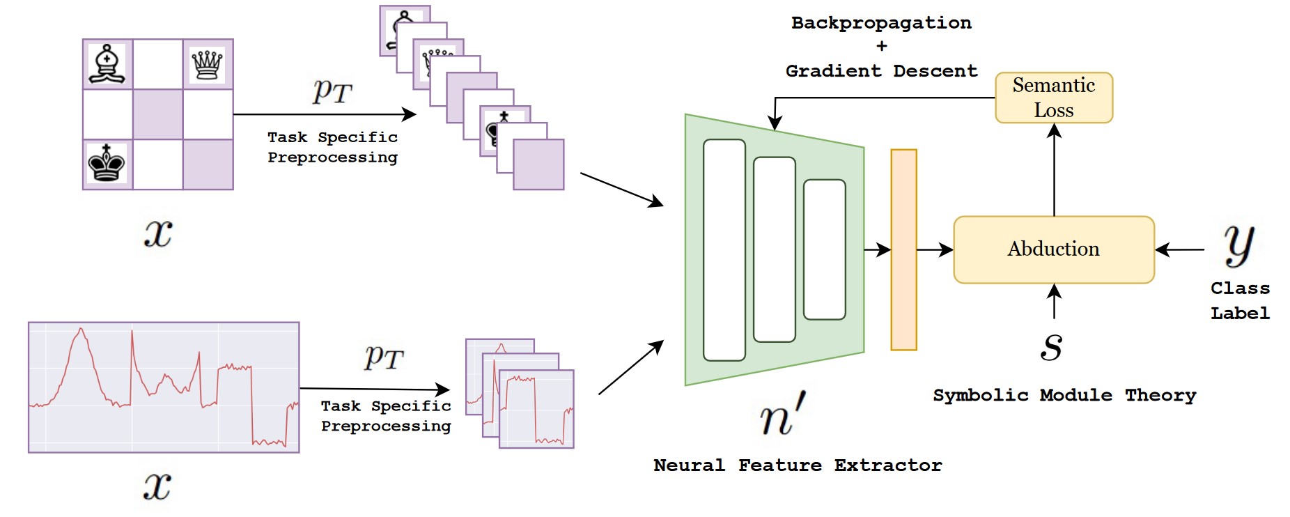
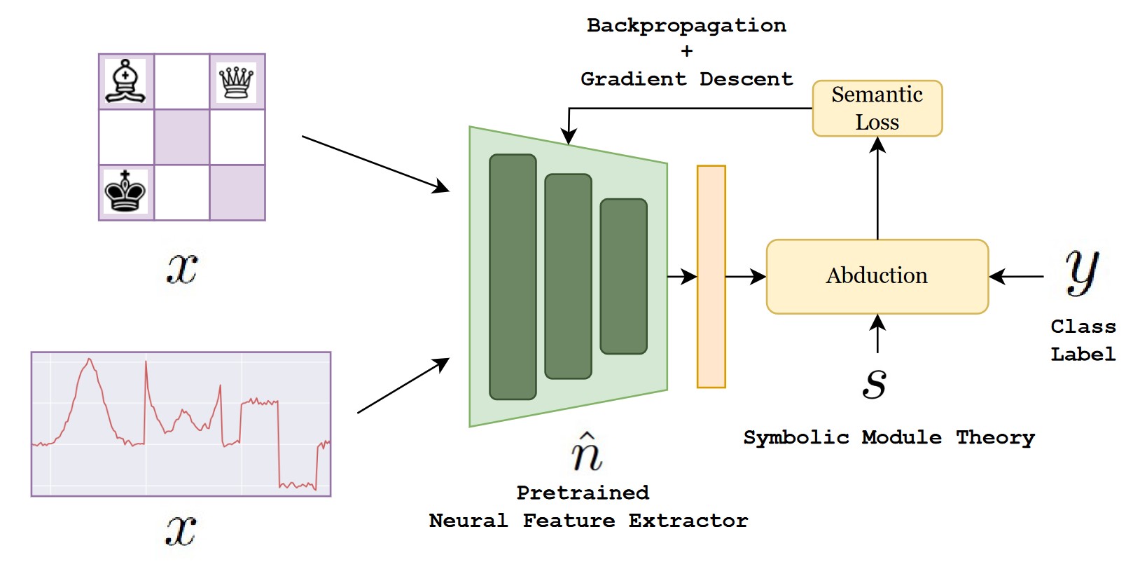
Figure 2: (a) $NEUROLOG$: the image input is pre-processed by segmenting out individual squares, thereby making the downstream learning with semantic loss easier. The diagram is for the chess problem described in (Tsamoura and Michael 2021). (b) ${NEUROLOG}^{-}$: the image input is no longer pre-processed but the feature extraction network is potentially imperfect.

The task specific pre-processing could be seen as a form of prior information about the features, for realistic applications it may not always be obvious what these functions should be. We consider pre-training as a simple alternative for introducing prior information about the features.

${NEUROLOG}$ without Pre-Processing

What is to be done if it is not possible to specify or implement the task-specific pre-processor $p_{T}$? Since the pre-processing step essentially constitutes prior information about the task, we can distinguish two kinds of implementations of $n$: one that is obtained with no prior knowledge (correctly, an uninformed prior); and one that is obtained without task-specific pre-processing but with task-independent prior information. For simplicity, we will denote these two models as implementing the functions $n_{0}$ (no prior) and $n_{1}$ (task-independent prior). The corresponding neuro-symbolic model are $s(n_{0}(\cdot))$ and $s(n_{1}(\cdot))$, which we denote by ${NEUROLOG}_{0}^{-}$ and ${NEUROLOG}_{1}^{-}$ (the minus superscript signifying that it denotes ${NEUROLOG}$ without pre-processing).

One option for $n_{1}$ is to start with prior values for parameters obtained from some form of pre-training. That is, suppose there exists an implementation $\hat{n}_{1}:\hat{{\cal X}}\mapsto\{0,1\}^{k}$, and the parameters of this model are modified using the data drawn from ${\cal X}$ to yield $n_{1}:{\cal X}\mapsto\{0,1\}^{k}$ that is reasonably consistent (defined using the loss function) with the constraints imposed by $s$. This may require ${\cal X}\subseteq\hat{{\cal X}}$, or at least a sufficient large overlap between ${\cal X}$ and $\hat{{\cal X}}$). Further, we would expect the neuro-symbolic model obtained in this way not to be as effective as one with task-specific pre-processing. But, it allows the practically useful prospect of implementing a form of $NEUROLOG$ of ‘feature-adaptation’ (see Fig. 2). The extent to which this can help when pre-processing is not possible is the focus of the experimental investigation below.

Experimental Evaluation

Aims

For brevity, we use $N(\cdot)$ to denote $NEUROLOG$ with pre-processing; $N_{0}^{-}$ to denote ${NEUROLOG}_{0}^{-}$ (that is, $NEUROLOG$ without pre-processing and without a pre-trained feature-extractor); and $N_{1}^{-}$ to denote ${NEUROLOG}_{1}^{-}$ (that is, $NEUROLOG$ without pre-processing and a with a pre-trained feature-extractors). We aim to investigate the following conjectures:

Pre-Processing.

If pre-processing is possible, then models constructed by $N$ are better than those constructed by $N_{0}^{-}$ and $N_{1}^{-}$;

Pre-Training.

If pre-processing is not possible, then models constructed by $N_{1}^{-}$ are better than models constructed by $N_{0}^{-}$.

The following clarifications are necessary: (a) By “better”, we will mean higher predictive accuracy and higher explanatory fidelity (a definition for this is in the Methods section); and (b) Using synthetic problems and simulated data, we are able to obtain $N_{1}^{-}$ models starting from progressively poorer pre-trained models. This allows us to examine qualifications to the conjectures, based on the corresponding $N_{1}^{-}$ models.

Materials

Problems

We report results from experiments conducted on two different problem domains: the Chess problem reported in (Tsamoura and Michael 2021) and synthetic time-series data obtained by controlled simulation.

Chess. We refer the reader to (Tsamoura and Michael 2021) for details of this problem and simply summarise the main aspects here. The raw data consists of a 3 $\times$ 3 chess board with 3 chess pieces – a black king and two distinct white pieces. Task-specific pre-processing involves a ‘segmentation’ step that separates each data-instance into the 9 squares in a pre-specified order. Each square corresponds to a (multi-valued) feature, with values indicating whether it is empty, or which of 7 other pieces it has (black king, white king, white rook, white knight, white pawn, white bishop, white knight). The logical theory encodes the conditions for class-labels denoting: safe, draw, and mate according to the usual rules of chess (or ‘illegal’ otherwise). In the terminology of this paper, this corresponds to $m$ Yes. definitions for each class-label (the number $m$ is different for each class) in terms of a disjunct of conjunctions of the 9 features (with $\bot$ = ‘illegal’).

We use the same data provided with and code adapted from the author’s implementation of $NEUROLOG$ for our experiments.
Time Series. We generate synthetic examples of simple time-series data, to resemble aspects of the Chess problem. Each time-series consists of three features in the form of different shapes, sampled from a pool of nine shapes: {Blank, SemiCircle, SquareWave, Triangle, Gaussian, Quadrant, Trapezium, Quatrefoil, W-wave}. Each shape spans 50 time steps and three of the these shapes are sampled and concatenated end-to-end to form one cycle. One time series is a periodic repetition of approximately 1.5 such cycles, extending over 256 time-steps. An example of some randomly generated time-series is shown in Fig. 3.

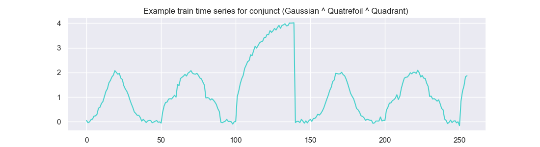
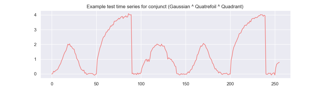
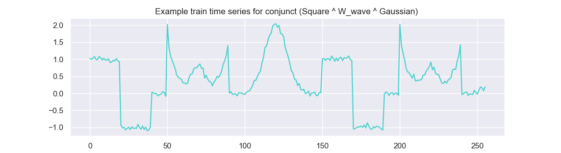
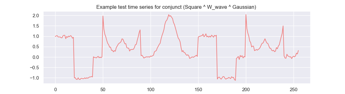
Figure 3: (a, b) Examples of randomly generated train and test time-series data for the conjunct (Gaussian $\land$ Quatrefoil $\land$ Quadrant). (c, d) Examples of randomly generated train and test time-series data for the conjunct (SquareWave $\land$ W_wave $\land$ Gaussian). Note that the order in which the shapes occur can be different between a train and test data point, as in (c, d).

As with the Chess data, it is possible to devise a ‘segmented’ input for $NEUROLOG$ that converts a time-series into 3 features in a pre-defined order (left-to-right; $f_{1}$, $f_{2}$, $f_{3}$). A symbolic ‘theory’ about the data is constructed as follows, by assuming a set of 4 class-labels (A,B,C, and D). A definition of a class-label essentially consists of a random number of conjuncts, each with 3 randomly chosen shapes (the details are in “Methods”). Data for each class label are then generated to be consistent with the target theory for that class label.

Machines and Environments

All the experiments were run on machines with Intel(R) Xeon(R) E5-2698 v4 CPU end to end with an allocation of 8GB of memory. We use PyTorch to program the Neural Networks. $NEUROLOG$ uses A-System (Nuffelen and Kakas 2001) running over SICStus Prolog 4.5.1 for the abduction process. However, for our experiments, we cache the abductive feedback for all the three classes in the chess domain in text files and use those for calculating the semantic loss.

Methods

We first describe some procedures required for conducting the experiments.

Generation of Time-Series Problems

Recall the time-series problems consist of a periodically repeating pattern of 3 shapes drawn from a possible set of 9 shapes. For the experiments, we need, a symbolic theory and data instances (time-series) consistent with the symbolic theory. For our experiments, the symbolic theory $s$ will assign one of 4 class-labels to data instances. The definition used by $s$ for each class-label is obtained as follows:

1. We partition the set of nine shapes into groups of three features each. These groups are assigned to one of the three features each. This is done randomly. Each feature can only take one of the shapes from the assigned group at a time as a possible value.

2. Next, we randomly sample one shape from the three groups each. The combination of these three shapes forms a randomly sampled conjunct.

3. Next, we decide the number of conjuncts to be assigned to each class. We define the parameters lower bound and upper bound. For each class in the theory, number of conjuncts to be assigned is determined by randomly sampling a number from [lower bound, upper bound). Note that different classes can have different number of conjuncts.

4. For each class, we randomly sample the conjuncts required as discussed in Step 1. We take care that conjuncts do not overlap between classes.

An example of a randomly sampled $s$ is given below:

The result of these steps is a randomly drawn symbolic theory about the data-instances. Using this theory, data-instances consistent with the theory are generated as follows:

1. For each conjunct assigned to a particular class, we generate a cycle by concatenating the shapes in the conjunct. Let’s denote these three shapes as $\psi_{1}$, $\psi_{2}$ and $\psi_{3}$.

2. To differentiate the test data from the train data, we concatenate the shapes in the order $\psi_{1},\psi_{2},\psi_{3}$ for the training data, whereas for test data, 30% of the time series are constructed by concatenating them in the same order and the rest are constructed by concatenating them them in the order $\psi_{1},\psi_{3},\psi_{2}$ (see Fig. 3).

3. The cycle is repeated to get a total of 10000 time steps for the training data and 750 time steps for testing data.

4. We add Gaussian noise to these time series to add randomness.

5. These time series are then cut into non-overlapping sequences of length 256 each giving us a total of 39 samples per conjunct for training data and 9 samples for testing data. Note that the total amount of training and test data for the time-series experiments depends on the total number of conjuncts in the theory, which varies across random runs.

Task-independent Pre-training

The steps followed for testing the conjectures is straightforward: is:

• Repeat $R$ times:

  1. For $T=$ $Chess$, $Time-Series$

     1. Randomly generate training and test data as described above (applicable only for time series data)

     2. Let $s_{T}$ be the symbolic theory for task $T$

     3. Let $p_{T}$ be the task-specific pre-processor for task $T$ and $N$ denote the $NEUROLOG$ model obtained using the training data, along with $s_{T}$ and the pre-processor $p_{T}$

     4. Let $\hat{n}_{\alpha}$ be an approximate pre-trained model for the features ($\alpha$ denotes an approximation parameter: see details below) and $N_{1,\alpha}^{-}$ be the ${NEUROLOG}^{-}$ model obtained using the training data, along with $s_{T}$ and with parameters of the neural feature-extractor initialised using the parameters of $\hat{n}_{\alpha}$

     5. Let $N_{0}^{-}$ be the ${NEUROLOG}^{-}$ model obtained using the training data, along with $s_{T}$ and with parameters of a completely untrained neural feature-extractor;

     6. Record estimates of predictive accuracy and explanatory fidelity of $N$, $N_{1,\alpha}^{-}$, and $N_{0}^{-}$ on the test data (see details below)

  2. Test the “Pre-Processing” conjecture by comparing the (mean) estimates of predictive accuracy and explanatory fidelity for $N$ against those obtained for $N_{1,\cdot}^{-}$ and $N_{0}^{-}$

  3. Test the “Pre-Training” conjecture by comparing the (mean) estimates of predictive accuracy and explanatory fidelity for $N_{1,\cdot}^{-}$ againsts those obtained for $N_{0}^{-}$.

The following details are relevant:

• For all experiments $R=5$;

• Training and test data sizes for Chess are 9000 and 2000 respectively. For Time Series the corresponding numbers are about 1000 and 200 (numbers vary due to the theory being sampled randomly); We use lower bound = 5 and upper bound = 8.

• We restrict $\alpha$ to $0.1$, $0.2$ and $0.3$; denoting low, medium and high levels of difference with the true feature detector

• Predictive accuracy is the usual ratio of correct predictions to total instances predicted. The estimates are from predictions on the test data instances.

• Explanatory fidelity refers to the ratio of correctly explained instances to the total number of instances. An instance is correctly explained if the conjunct used to generate the class label is the (only) conjunct that is determined to be true given the features extracted by the neural layer;

• We report the metric after taking a running average to 100.

• Model performance is represented by the pair $(P,E)$, where $P$ denotes predictive accuracy and $E$ denotes explanatory fidelity. Let model $M1$ have performance $(P1,E1)$ and model $M2$ have performance $(P2,E2)$. If $P1>P2$ and $E1>E2$ then we will say model $M1$ is better than model $M2$.

		Pred Acc.(%)	Expl Fid.(%)
$N$		95.41 (0.66)	94.67 (0.69)
$N_{1,\alpha}^{-}$	$\alpha=0.1$	84.71 (1.34)	62.71 (3.80)
	$\alpha=0.2$	80.31 (1.67)	48.12 (5.07)
	$\alpha=0.3$	78.79 (2.68)	43.32 (4.17)
$N_{0}^{-}$		79.88 (1.57)	0.10 (0.13)

(a) Chess

		Pred Acc.(%)	Expl Fid.(%)
$N$		100 (0.00)	100 (0.00)
$N_{1,\alpha}^{-}$	$\alpha=0.1$	82.07 (6.59)	76.05 (10.23)
	$\alpha=0.2$	81.48 (4.44)	76.08 (7.78)
	$\alpha=0.3$	81.56 (4.61)	75.37 (10.28)
$N_{0}^{-}$		75.79 (11.86)	36.81 (16.85)

(b) Time Series

Table 1: Performance of models with pre-processsing ($N$); without pre-processing but with pre-training ($N_{1,\alpha}^{-}$); without pre-processing and without pre-training ($N_{0}^{-}$. “Pred. Acc.” refers to (mean) predictive accuracy; “Expl. Fid.” refers to (mean) explanatory fidelity. The number in brackets is the standard deviation. Lower values of $\alpha$ indicates that the pre-trained approximation $\hat{n}_{\alpha}$ is closer to the correct model for feature-subset identification (the values of $\alpha$ correspond to low, medium, and high-levels of difference between predictions from $\hat{n}$ and the correct prediction.

Approximate Pre-Training ($\alpha$)

Approximate models for pre-training are generated by deliberately altering feature-labels. The value of $\alpha$ defines the percentage of feature labels that are corrupted during the time of pretraining.

• For the chess experiment, the position and identity of each of the three pieces has a probability of $\alpha$ to be changed to one of the other possible values which is randomly chosen.

• For the time series experiment, the labels for each of the three shapes has a probability of $\alpha$ of being changed to one of the other two possible values (i.e. the remaining two values from the same ”group”).

Results

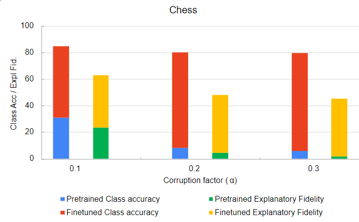
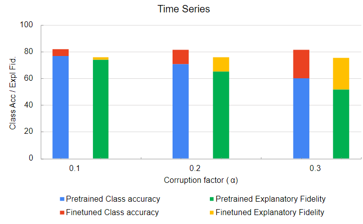
Figure 4: Increase in Prediction Accuracy and Explanatory Fidelity of the approximate models after finetuning with semantic loss

The main results of the empirical study are tabulated in Tables 1(a), (b). The tabulations suggest the following: (a) If pre-processing is possible, then clearly better models (that is, with higher predictive accuracy and higher explanatory fidelity) result from using task-specific pre-processing than from using task-independent pre-training. (b) If pre-processing is not possible, then it is usually better to employ a pre-trained model than to start with an uninformed model; (c) As expected, as the pre-trained approximation becomes progressively uninformative (medium to high values of $\alpha$), performance on predictive and explanatory fronts decreases. However, even with with fairly poor initial approximation, explanatory fidelity remains substantially better than starting with an uninformed model; and (d) The loss in performance due to lack of pre-processing can be offset to some extent through the use of pre-training, especially with a good initial approximation (low value of $\alpha$). Taken together, these results provide empirical support for the Pre-Processing and Pre-Training conjectures.

We now turn to a more detailed finding from the experiments for cases when pre-processing is not an option. It is evident from Table 1 that there is a substantial ‘gap’ between the predictive accuracy and explantory fidelity estimate. This is more pronounced as the pre-trained approximator gets worse; and especially obvious for the model $N_{0}^{-}$ that does not employ a pre-trained approximator. That is, there are more predictions that are correct, but for the wrong reasons. We find that this is because without sufficient prior information about the features, the neural networks training process allows a convergence to arbitrary conjuncts that are associated with the correct class label. This tends to keep predictive accuracy from falling, but results in substantially poorer accuracy of correct feature-identification. This is shown for Chess in Table 2, where the effect is especially pronounced (the results from the model with pre-processing are shown purely for reference). We also show the comparision between the approximate model $n_{\alpha}$ and $N_{1,\alpha}^{-}$ in Fig. 4. The increase in explanatory fidelity is clearly visible and is more significant in the case of chess domain.

Model		Mean F-score
		$f_{1}$	$f_{2}$	$f_{3}$	$f_{4}$	$f_{5}$	$f_{6}$	$f_{7}$	$f_{8}$	$f_{9}$
$N_{1,\alpha}^{-}$	$\alpha=0.1$	0.94	0.95	0.91	0.96	0.98	0.95	0.95	0.95	0.94
	$\alpha=0.2$	0.94	0.93	0.89	0.94	0.97	0.91	0.91	0.93	0.92
	$\alpha=0.3$	0.91	0.94	0.85	0.92	0.89	0.91	0.88	0.86	0.92
$N_{0}^{-}$		0.22	0.13	0.29	0.50	0.58	0.30	0.30	0.25	0.36
$N$		0.99	0.99	0.99	0.99	0.99	0.99	0.99	0.99	0.99

Table 2: Comparing mean F1-scores for feature-prediction in the chess domain. The models are as in Table 1.

The symbolic theory for Chess is significantly more complex than the ones used for the Time Series data (the conjunct size in the Chess theory is 9, compared to 3 for Time Series and the number of conjuncts belonging to each class in Chess is also significantly higher). We conjecture that if pre-processing is not possible, then for complex theories pre-training to some extent may be needed to attain reasonable levels of explanatory fidelity.

Related Work

While the impressive performance of deep learning architectures underscores the pattern recognition capabilities of neural networks, deep models still struggle to imbibe explicit domain knowledge and perform logical reasoning. Symbolic systems on the other hand are adept at reasoning over explicit knowledge but can only ingest symbolic inputs. The community has been striving to combine the pattern recognition capabilities of neural networks with the reasoning and knowledge representation power of symbolic techniques. Towards this end, one line of attack has been to feed knowledge rich symbolic features explicitly as inputs to a neural network instead of relying on the network to learn these features from low level data (Lodhi 2013; Dash et al. 2018; Dash, Srinivasan, and Vig 2021). These techniques are useful when i) Knowledge regarding high level symbolic features is easily accessible and ii) The high level features are easily computed from low level data.

The second line of attack involves using a neural network to ingest noisy unstructured real world data (Images, Time Series, Speech or Text) and predict the symbolic features that can be ingested by a symbolic model (Sunder et al. 2019). In many situations, although knowledge about the appropriate symbolic features is available and a symbolic theory for making predictions exists, the raw input data is not easily transformed into the symbolic inputs necessary for the symbolic theory. Doing so accurately via neural networks would require a large volume of annotated data for each symbolic input which is often infeasible to obtain for a new domain. Recent efforts towards end-to-end neuro symbolic training (Manhaeve et al. 2018; neurolog) aim to address this limitation by obviating the need to learn neural feature detectors in isolation prior to integration with the symbolic theory. This paper is concerned with this type of neuro symbolic architecture.

Among systems that attempt to replace symbolic computations with differentiable functions (Gaunt et al. 2017) develop a framework for creation of end-to-end trainable systems that learn to write interpretable algorithms with perceptual components, however the transformation of the theory into differentiable functions is restricted to work for a subset of possible theories. Logic Tensor Networks (LTNs)(Donadello, Serafini, and d’Avila Garcez 2017) integrate neural networks with first-order fuzzy logic to allow for logically constrained learning from noisy data. Along similar lines the DeepProbLog(Manhaeve et al. 2018) system introduces the notion of neural predicates to probabilistic logic programming(Raedt, Kimmig, and Toivonen 2007) that allows for backpropogation across both the neural and symbolic modules. The ABL (Dai et al. 2019) system was the first to use abductive reasoning to refine neural predictions via consistency checking between the predicted neural features and the theory. This system was recently refined by using a similarity based consistency optimization (Huang et al. 2021), that relies on assumptions about the inter class and intra class neural features. Recently Abductive Meta-Interpretive Learning(Dai and Muggleton 2021) was proposed to jointly learn neural feature predictors and the logical theory via induction and abduction. While the above abduction based approaches require iterative retraining of the neural module, and only utilize some of the abduced inputs for backpropagation, the NEUROLOG system (Tsamoura and Michael 2021) uses the complete set of abduced inputs and backpropogates errors using Semantic loss (Xu et al. 2018) that more fully capture theory semantics.

Concluding Remarks

A limitation of prior abduction based neuro-symbolic approaches is that they only experiment with cleanly delineated inputs and the neural network does not have the additional burden of learning where to attend while predicting a feature. However, in many situations such feature delineation is not possible. Consider a dataset of images containing multiple objects at random locations and a logical feature corresponding to whether the number of cars in an image is greater than a threshold. In this case it is not obvious how one would slice the image, and therefore the burden falls on the neural network to extract this feature directly from the full image. We demonstrate with NEUROLOG that for such cases where the network is forced to operate on the full inputs, and is trained only with semantic loss, it fails to learn the correct sub-symbolic features but can still yield high predictive accuracy. We further show that the resulting model can be improved to a degree with even partially pre-trained neural models with the extent of the improvement dependent on the quality of the initial pre-training. This is very useful for situations where the same theory applies to multiple domains with varying distributions of sub-symbolic features. The imperfect feature detectors trained on a different distribution can be significantly improved upon with semantic loss and abductive feedback. The results from our experiments reinforce the message: Pre-process. Otherwise pre-train.

Appendix

Data

Using MNIST Digits for Chess Data

As done in the original NEUROLOG experiments we use the MNIST handwritten digits dataset for performing experiments on the chess domain. Each of the eight possible values for a position on the 3 $\times$ 3 chess board is mapped to a number from 0 - 7 as given: Empty - 0, Black King - 1, White Rook - 2, White Bishop - 3, White Knight - 4, White King - 5, White Pawn - 6, White Queen - 7. An image of a chess board is made by placing an instance of an image of a digit from the MNIST dataset corresponding to a chess piece (or Empty) at it’s respective position. Each MNIST image has a dimension of 28 $\times$ 28. Hence, an image of a chess board has the dimensions 84 $\times$ 84. Fig. 5 shows an example image of a chess board in a given configuration.

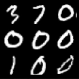
Figure 5: Image used for a chess board having a White Bishop at $(1,1)$, a White Queen at $(1,2)$ and a Black King at $(3,1)$

Logical Theory Used for Time Series Experiments

Methods section in the main paper describes how we randomly sample logical theories for experiments on time-series data. Table 3 shows one such example theory where the Class column contains the four classes that we use for time-series domain experiments and the Conjuncts columns contains disjunction of conjuncts assigned to a given class. This theory was sampled using lower bound = 2 and upperbound = 5. For brevity. we use numbers to represent shapes: 0 - Blank, 1 - SemiCircle, 2 - Triangle, 3 - Gaussian, 4 - SquareWave, 5 - Quadrant, 6 - Trapezium, 7 - Quatrefoil, 8 - W-wave.

Class	Conjuncts
A	$(2\land 0\land 7)\lor(4\land 3\land 6)\lor(1\land 5\land 8)$
B	$(4\land 5\land 8)\lor(1\land 0\land 7)$
C	$(2\land 5\land 6)\lor(1\land 3\land 7)\lor(4\land 0\land 8)$
D	$(1\land 5\land 7)\lor(4\land 1\land 6)$

Table 3: Example Theory for an experiment on Time-Series Data

Shapes used for Time-Series Experiments

The data used for time-series experiments is made by composing shapes derived from a set of 9 shapes which are generated procedurally. Each shape spans 50 time-steps. Fig. 6 shows all of the 9 shapes and the equations used to generate them. 3 of such shapes are joined together and a guassian noise of mean 0 and standard deviation of 0.05 is added to make the timeseries.

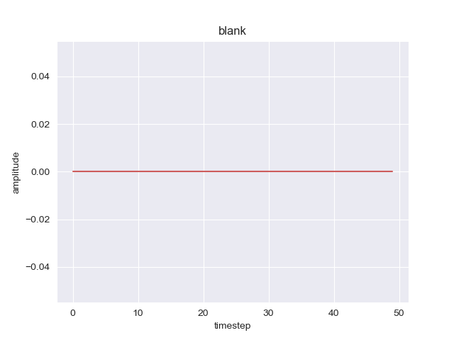
(a) Blank

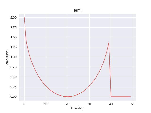
(b) SemiCircle

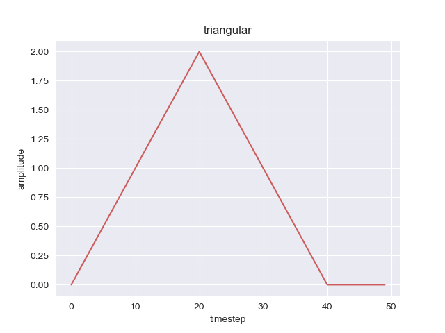
(c) Triangle

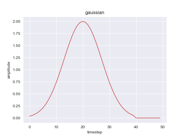
(d) Gaussian

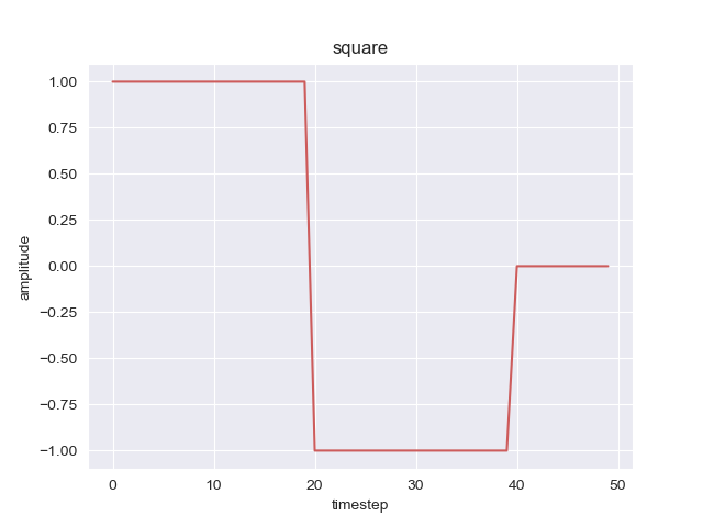
(e) SquareWave

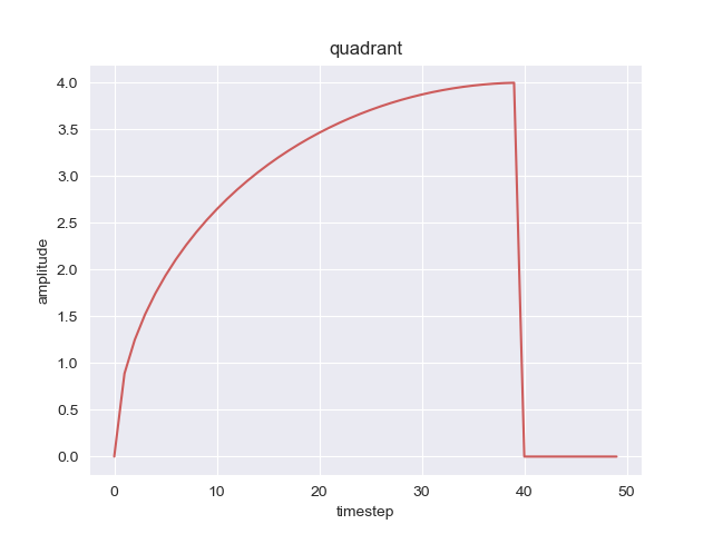
(f) Quadrant

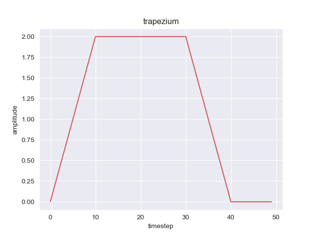
(g) Trapezium

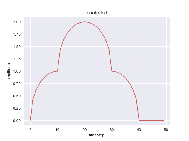
(h) Quatrefoil

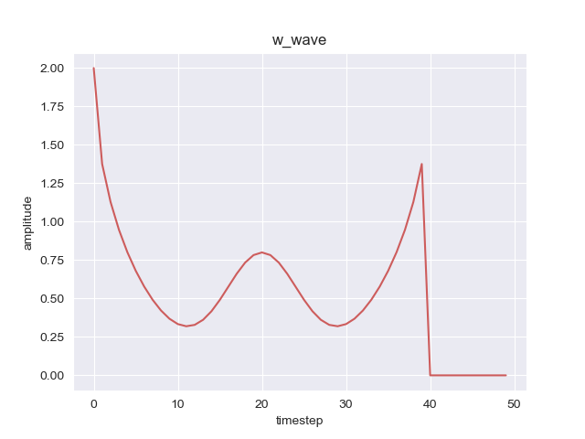
(i) W-wave

Figure 6: Figures and equations of 9 shapes used for making the synthetic time-series data

Segmenting Features for NEUROLOG Experiments on Time-Series Data

Running $NEUROLOG$ on the time-series domain requires a neat segmentation of the three features (shapes) present in a time-series. Each shape spans 50 time-steps. We use this knowledge to perform the segmentation. For $NEUROLOG$ experiments, we split the training and test series in lengths of 150 instead of 256. This is to ensure that the start of each time-series data point coincides with the start of a shape. Then we break down the 150 time-steps into 3 consecutive segments of 50 time-steps each which correspond to the three features.

Corrupting Feature Labels

Corrupting Piece Information in Chess Data

Let Let $\mathcal{P}$ be the set of all chess pieces in the chess domain $\cal C$ be a set defined as below and $\alpha$ with is the corruption factor

$\mathcal{P}=\{b(k),w(r),w(b),w(n),w(k),w(p),w(q)\}$

$\mathcal{C}=\{1,2,3\}$

In the chess domain, a feature label for a particular instance of a chess board can be represented as given below where where $P_{i}\in\mathcal{P}$ are the identities of the chess piece and $X_{i},Y_{i}\in\mathcal{C}$ are their coordinates on the chess board, with the constraint that one of the pieces is a black king and the other two pieces are distinct white pieces.

$\{at(P_{1},(X_{1},Y_{1})),at(P_{2},(X_{2},Y_{2})),at(P_{3},(X_{3},Y_{3}))\}$

To corrupt the feature label for a particular instance of chess data, the steps given below are executed, each with a probability of $\alpha$.

$P_{i}\leftarrow p;p\sim\mathcal{P}/\{P_{i}\}$ $\forall i\in\{1,2,3\}$

$X_{i}\leftarrow x;x\sim\mathcal{C}/\{X_{i}\}$ $\forall i\in\{1,2,3\}$

$Y_{i}\leftarrow y;y\sim\mathcal{P}/\{Y_{i}\}$ $\forall i\in\{1,2,3\}$

Corrupting Shape labels for Time-Series Data

As described in the main paper, the set of 9 shapes is randomly partitioned into a 3 sets of 3 shapes and each of these sets is assigned to the three features of the time-series. Let $\mathcal{S}_{1}$, $\mathcal{S}_{2}$ and $\mathcal{S}_{3}$ be these three sets.

Each of the features can take values from the respective set of shapes. For a particular experiment, let $v_{1},v_{2},v_{3}$ represent the values taken by Feature 1, Feature 2 and Feature 3 respectively. Then $v_{1}\in\mathcal{S}_{1}$, $v_{2}\in\mathcal{S}_{2}$ and $v_{2}\in\mathcal{S}_{3}$. Further, a feature label for an instance of the time-series data can be represented as $\{v_{1},v_{2},v_{3}\}$.

Let the training data be represented by $\mathcal{D}$. For corruption, the training dataset $\mathcal{D}$ is divided in a ratio of $\alpha:(1-\alpha)$. Let the two divisions be represented as $\mathcal{D}_{\alpha}$ and $\mathcal{D}_{1-\alpha}$. The feature label $\{v_{1\alpha},v_{2\alpha},v_{3\alpha}\}$ of every data point in $\mathcal{D}_{\alpha}$ is corrupted as:

$v_{1\alpha}\leftarrow v;v\sim\mathcal{S}_{1}/\{v_{1\alpha}\}$

$v_{2\alpha}\leftarrow v;v\sim\mathcal{S}_{2}/\{v_{2\alpha}\}$

$v_{3\alpha}\leftarrow v;v\sim\mathcal{S}_{3}/\{v_{3\alpha}\}$

$\mathcal{D}_{\alpha}$ with corrupted labels, denoted by $\hat{\mathcal{D}_{\alpha}}$ is then rejoined with $\mathcal{D}_{1-\alpha}$ and shuffled to form the corrupted training dataset $\hat{\mathcal{D}}$:

$\hat{\mathcal{D}}=\{\hat{\mathcal{D}_{\alpha}},\mathcal{D}_{1-\alpha}\}$

Network Architectures

Chess Experiments

The feature extractors use a 2D Convolutional Neural Network with ReLU activations for embedding the images in case of both $NEUROLOG$ and $NEUROLOG^{-}$.

$NEUROLOG$: We use the same model as used in the original implementation. The input to the network is a 28$\times$28 image and the output is a vector of length 8 for classifying among the 8 classes (7 chess pieces + empty class). The architecture is as given below:

• Embedding Layers

  • Conv2D (1, 6), 5$\times$5 filters, stride 1, padding 0

  • MaxPool2D, 2$\times$2 filters

  • ReLU

  • Conv2D (6,16), 5$\times$5 filters, stride 1, padding 0

  • MaxPool2D, 2$\times$2 filters

  • ReLU

• Classification MLP

  • FC (256, 120)

  • ReLU

  • FC (120, 84)

  • ReLU

  • FC (84, 8)

$NEUROLOG^{-}$: We use a network similar to the network used above with input and output layers slightly modified to support larger input and output sizes. The input to the network is an 84$\times$84 image, whereas the output is a vector of size 72 (9$\times$8). The first 8 outputs are used for classifying the first block of the chess board, next 8 outputs are used for classifying the second block and so on.

• Embedding Layers

  • Conv2D (1, 6), 5$\times$5 filters, stride 2, padding 0

  • MaxPool2D, 2$\times$2 filters

  • ReLU

  • Conv2D (6, 16), 5$\times$5 filters, stride 1, padding 0

  • MaxPool2D, 2$\times$2 filters

  • ReLU

• Classification MLP

  • FC (1024, 512)

  • ReLU

  • FC (512, 256)

  • ReLU

  • FC (256, 72)

Time Series Experiments

The feature extractors use a 1D Convolutional Neural Network with ReLU activations for embedding the images in case of both $NEUROLOG$ and $NEUROLOG^{-}$.

$NEUROLOG$: The input to the network is a signal of length 50 which is obtained from separating the shapes. The output is a vector of size 9 for classifying from one of the 9 shapes. The architecture is as given below:

• Embedding Layers

  • Conv1D (1, 32), kernel size 8 filters, stride 1, padding 0

  • ReLU

  • Conv1D (32, 32), kernel size 4, stride 1, padding 0

  • ReLU

  • MaxPool1D, kernel size 2

• Classification MLP

  • FC (640, 256)

  • ReLU

  • Dropout 0.5 probability

  • FC (256, 9)

$NEUROLOG^{-}$: We use a network similar to the network used above with input and output layers slightly modified to support a larger input size. The input to the network is a 256 length signal. The output is a vector of size 9 (3$\times$3). The first 3 outputs are used for determining the shape taken by the first feature from $\mathcal{S}_{1}$ of the signal, the next 3 for the determining the shape taken by Feature 2 from $\mathcal{S}_{2}$ and last three for determining the shape taken by Feature 3 from $\mathcal{S}_{3}$

• Embedding Layers

  • Conv1D (1, 32), kernel size 8 filters, stride 1, padding 0

  • ReLU

  • Conv1D (32, 32), kernel size 4, stride 1, padding 0

  • ReLU

  • MaxPool1D, kernel size 2

• Classification MLP

  • FC (3936, 256)

  • ReLU

  • Dropout 0.5 probability

  • FC (256, 9)

Deduction through Logical Theories

In this section, we describe how the outputs of the neural feature extractor are used for predicting the features and the final class.

Determining the Predicted Pieces in Chess Domain

1. From the outputs of the network, each of the 9 square are classified into belonging to one of the 8 states.

2. The abductive feedback is collected for all the three classes safe, mate, draw.

3. The predicted set of features is compared to all the abductive proofs in the abductive feedbacks in an attempt to find an exact match.

4. If a match is found the corresponding class is considered to be the predicted class. If a match is not found, the prediction is considered to be invalid.

Determining the Predicted Conjunct in Time-Series Domain

1. Categorical probability distributions are calculated (using softmax) over the three sets $\mathcal{S}_{1}$, $\mathcal{S}_{2}$ and $\mathcal{S}_{3}$. Let’s denote these distribution by $P_{\mathcal{S}_{1}}$, $P_{\mathcal{S}_{2}}$ and $P_{\mathcal{S}_{3}}$.

2. The probability of each of the conjuncts present in the theory is calculated by multiplying the probability of the component shapes. For eg. the probability of the conjunct $2\land 0\land 7$ in the theory given in Table 3 is calculated as $P_{\mathcal{S}_{1}}(2)\times P_{\mathcal{S}_{1}}(0)\times P_{\mathcal{S}_{1}}(7)$

3. The conjunct with the maximum probability is considered to be the predicted conjunct and the corresponding class is considered to be the predicted class.

Additional Training and Evaluation Details

In this section we talk about some additional details about the experiments:

Miscellaneous Details

• Cross Entropy Loss is used for pretraining the neural feature extractors in experiments on both chess and time-series domains.

• For the chess domain, we perform experiments on the ’BSV’ scenario as described in NEUROLOG (Tsamoura, Hospedales, and Michael 2021) only. We DO NOT investigate the ’NGA’ and ’ISK’ scenarios.

• For chess experiments we use all 9000 data points provided in the train data for training and 2000 randomly sampled data points from the test data for evaluation.

Hyperparameters

Table 4 lists further details and hyperparameters used in the experiments

	$NEUROLOG$	$NEUROLOG^{-}$
		Pretraining	Finetuning
Chess Experiments
Learning Rate	0.001	0.0001	0.00001
Optimizer	Adam	Adam	Adam
Train Epochs	15	40	15
Data Transforms	MinMax Scaling	MinMax Scaling	MinMax Scaling
Batch Size	1	64	1
Time Series Experiments
Learning Rate	0.0001	0.0001	0.0001
Optimizer	Adam	Adam	Adam
Train Epochs	300	200	300
Data Transforms	Z Normalization	Z Normalization	Z Normalization
Batch Size	64	64	64
Upper Bound	8	8	8
Lower Bound	5	5	5

Table 4: Experimental Details for the Experiments. MinMax Scaling is done between [-0.5,0.5]

Additional Experiments and Results

We further probe the effectiveness of $NEUROLOG^{-}$ on feature extractors pretrained with higher levels of noise in the time-series domain. We increase the level of corruption from 0.1 to 0.6 in steps of 0.1. Table 5 shows the results on the same.

Model		Class acc.	Expl fid.
$N$		100 (0.00)	100 (0.00)
$N_{1,\alpha}^{-}$	$\alpha=0.1$	82.07 (6.59)	76.05 (10.23)
	$\alpha=0.2$	81.48 (4.44)	76.08 (7.78)
	$\alpha=0.3$	81.56 (4.61)	75.37 (10.28)
	$\alpha=0.4$	76.80 (7.73)	67.70 (12.57)
	$\alpha=0.5$	69.12 (7.24)	52.09 (11.44)
	$\alpha=0.6$	62.71 (2.77)	29.88 (3.04)
$N_{0}^{-}$		75.79 (11.86)	36.81 (16.85)

Table 5: Class accuracy and Explanatory Fidelity for decreasing quality of feature extractor (by increasing corruption $\alpha$).

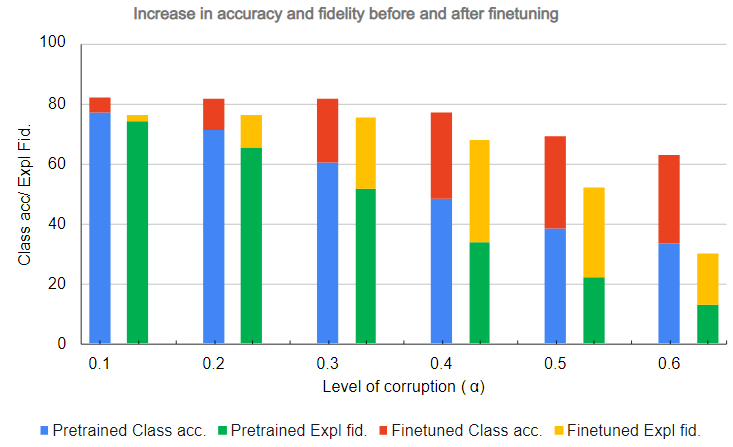
Figure 7: Pretrain and Finetune Class accuracy and Explanatory fidelity for different levels of corruption

Fig. 7 shows that the relative improvement using the semantic loss increases as the quality of feature extractors worsens, till a point. For the time series data, this maxima lies between $\alpha$ 0.4 and 0.5 with a gain of 28-33 % in both class accuracy and exploratory fidelity.

References

- Dai and Muggleton (2021) Dai, W.; and Muggleton, S. H. 2021. Abductive Knowledge Induction from Raw Data. In Zhou, Z., ed., Proceedings of the Thirtieth International Joint Conference on Artificial Intelligence, IJCAI 2021, Virtual Event / Montreal, Canada, 19-27 August 2021, 1845–1851. ijcai.org.
- Dai et al. (2019) Dai, W.; Xu, Q.; Yu, Y.; and Zhou, Z. 2019. Bridging Machine Learning and Logical Reasoning by Abductive Learning. In Wallach, H. M.; Larochelle, H.; Beygelzimer, A.; d’Alché-Buc, F.; Fox, E. B.; and Garnett, R., eds., Advances in Neural Information Processing Systems 32: Annual Conference on Neural Information Processing Systems 2019, NeurIPS 2019, December 8-14, 2019, Vancouver, BC, Canada, 2811–2822.
- Dash et al. (2022) Dash, T.; Chitlangia, S.; Ahuja, A.; and Srinivasan, A. 2022. A review of some techniques for inclusion of domain-knowledge into deep neural networks. Scientific Reports, 12.
- Dash, Srinivasan, and Vig (2021) Dash, T.; Srinivasan, A.; and Vig, L. 2021. Incorporating symbolic domain knowledge into graph neural networks. Mach. Learn., 110(7): 1609–1636.
- Dash et al. (2018) Dash, T.; Srinivasan, A.; Vig, L.; Orhobor, O. I.; and King, R. D. 2018. Large-Scale Assessment of Deep Relational Machines. In Riguzzi, F.; Bellodi, E.; and Zese, R., eds., Inductive Logic Programming - 28th International Conference, ILP 2018, Ferrara, Italy, September 2-4, 2018, Proceedings, volume 11105 of Lecture Notes in Computer Science, 22–37. Springer.
- Donadello, Serafini, and d’Avila Garcez (2017) Donadello, I.; Serafini, L.; and d’Avila Garcez, A. S. 2017. Logic Tensor Networks for Semantic Image Interpretation. In Sierra, C., ed., Proceedings of the Twenty-Sixth International Joint Conference on Artificial Intelligence, IJCAI 2017, Melbourne, Australia, August 19-25, 2017, 1596–1602. ijcai.org.
- Gaunt et al. (2017) Gaunt, A. L.; Brockschmidt, M.; Kushman, N.; and Tarlow, D. 2017. Differentiable Programs with Neural Libraries. In Precup, D.; and Teh, Y. W., eds., Proceedings of the 34th International Conference on Machine Learning, ICML 2017, Sydney, NSW, Australia, 6-11 August 2017, volume 70 of Proceedings of Machine Learning Research, 1213–1222. PMLR.
- Huang et al. (2021) Huang, Y.-X.; Dai, W.-Z.; Cai, L.-W.; Muggleton, S.; and Jiang, Y. 2021. Fast Abductive Learning by Similarity-based Consistency Optimization. In Beygelzimer, A.; Dauphin, Y.; Liang, P.; and Vaughan, J. W., eds., Advances in Neural Information Processing Systems.
- Lodhi (2013) Lodhi, H. 2013. Deep Relational Machines. In ICONIP.
- Manhaeve et al. (2018) Manhaeve, R.; Dumancic, S.; Kimmig, A.; Demeester, T.; and De Raedt, L. 2018. DeepProbLog: Neural Probabilistic Logic Programming. In Bengio, S.; Wallach, H.; Larochelle, H.; Grauman, K.; Cesa-Bianchi, N.; and Garnett, R., eds., Advances in Neural Information Processing Systems, volume 31. Curran Associates, Inc.
- Muggleton and Michie (1997) Muggleton, S.; and Michie, D. 1997. Machine Intelligibility and the Duality Principle. In Software Agents and Soft Computing: Towards Enhancing Machine Intelligence, Concepts and Applications, 276–292. Berlin, Heidelberg: Springer-Verlag. ISBN 3540625607.
- Nuffelen and Kakas (2001) Nuffelen, B. V.; and Kakas, A. C. 2001. A-system: Declarative Programming with Abduction. In LPNMR.
- Raedt, Kimmig, and Toivonen (2007) Raedt, L. D.; Kimmig, A.; and Toivonen, H. 2007. ProbLog: A Probabilistic Prolog and Its Application in Link Discovery. In Veloso, M. M., ed., IJCAI 2007, Proceedings of the 20th International Joint Conference on Artificial Intelligence, Hyderabad, India, January 6-12, 2007, 2462–2467.
- Ribeiro, Singh, and Guestrin (2016) Ribeiro, M. T.; Singh, S.; and Guestrin, C. 2016. ”Why Should I Trust You?”: Explaining the Predictions of Any Classifier. Proceedings of the 22nd ACM SIGKDD International Conference on Knowledge Discovery and Data Mining.
- Schwitter (2010) Schwitter, R. 2010. Controlled Natural Languages for Knowledge Representation. In Coling 2010: Posters, 1113–1121. Beijing, China: Coling 2010 Organizing Committee.
- Sunder et al. (2019) Sunder, V.; Srinivasan, A.; Vig, L.; Shroff, G.; and Rahul, R. 2019. One-shot Information Extraction from Document Images using Neuro-Deductive Program Synthesis. CoRR, abs/1906.02427.
- Tsamoura and Michael (2021) Tsamoura, E.; and Michael, L. 2021. Neural-Symbolic Integration: A Compositional Perspective. In AAAI Conference on Artificial Intelligence.
- Xu et al. (2018) Xu, J.; Zhang, Z.; Friedman, T.; Liang, Y.; and den Broeck, G. V. 2018. A Semantic Loss Function for Deep Learning with Symbolic Knowledge. In Dy, J. G.; and Krause, A., eds., Proceedings of the 35th International Conference on Machine Learning, ICML 2018, Stockholmsmässan, Stockholm, Sweden, July 10-15, 2018, volume 80 of Proceedings of Machine Learning Research, 5498–5507. PMLR.