Thermalization and disentanglement with a nonlinear Schrödinger equation

Abstract

We study a recently proposed modified Schrödinger equation having an added nonlinear term. For the case where a stochastic term is added to the Hamiltonian, the fluctuating response is found to resemble the process of thermalization. Disentanglement induced by the added nonlinear term is explored for a system made of two coupled spins. A butterfly-like effect is found near fully entangled states of the spin-spin system. A limit cycle solution is found when one of the spins is externally driven.

I Introduction

In 1935 Schrodinger_807 Schrödinger has identified a self-inconsistency in the quantum to classical transition process Penrose_4864 ; Leggett_939 ; Leggett_022001 , which became known as the problem of quantum measurement. This problem is related to the phenomenon of quantum entanglement. Exploring possible mechanisms of disentanglement, may help resolving this long-standing problem.

Processes such as disentanglement require nonlinear time evolution. A variety of nonlinear terms Geller_2111_05977 that can be added to the Schrödinger equation have been explored before Weinberg_336 ; Weinberg_61 ; Doebner_397 ; Doebner_3764 ; Gisin_5677 ; Kaplan_055002 ; Munoz_110503 . In most previous proposals, the purpose of the added nonlinear terms is to generate a spontaneous collapse Bassi_471 .

Here we explore a recently proposed modified Schrödinger equation having an added nonlinear term Buks_355303 (see section II). The proposed equation can be constructed for any physical system having Hilbert space of finite dimensionality, and it does not violate unitarity of the time evolution.

The effect of the added term on the dynamics of a single spin 1/2 is studied in section III. The spin’s response to an applied fluctuating magnetic field is found to mimic the process of thermalization Diosi_451 ; Molmer_524 ; Dalibard_580 ; Semin_063313 (see section IV). Disentanglement induced by the nonlinear term is explored with two coupled spins (see section V). A butterfly-like effect is found near fully entangled spin-spin states.

The system can become unstable when one spin is externally driven (see section VI). Limit cycle solutions for the modified Schrödinger equation are found in the instability region. The instability of the modified Schrödinger equation is closely related to an instability found with a similar spin-spin system Levi_053516 , when the equations of motion generated by the standard Schrödinger equation are analyzed using the mean field approximation breuer2002theory ; Drossel_217 ; Hicke_024401 ; Klobus_034201 .

II The modified Schrödinger equation

Let $\mathcal{H}$ be a time-independent Hermitian Hamiltonian of a given physical system. Consider a modified Schrödinger equation for the state vector $\left|\psi\right\rangle$ given by Buks_355303

$$\frac{\mathrm{d}}{\mathrm{d}t}\left|\psi\right\rangle=\left(-i\hbar^{-1}\mathcal{H}+\gamma_{\mathrm{D}}M_{\mathrm{D}}\right)\left|\psi\right\rangle\;,$$ (1)

where $\mathrm{d}/\mathrm{d}t$ is a time derivative. In the added (to the standard Schrödinger equation) term $\gamma_{\mathrm{D}}M_{\mathrm{D}}$, the rate $\gamma_{\mathrm{D}}$ is a positive coefficient, and the operator $M_{\mathrm{D}}$ is derived from a given non-zero state vector $\left|\Psi\right\rangle$ according to (the state vector $\left|\Psi\right\rangle$ is not required to be normalized)

$$M_{\mathrm{D}}=-\sqrt{\frac{\left\langle\Psi\right.\left|\Psi\right\rangle}{1-\left\langle\mathcal{P}\right\rangle}}\left(\mathcal{P}-\left\langle\mathcal{P}\right\rangle\right)\;,$$ (2)

where the projection operator $\mathcal{P}$ is given by

$$\mathcal{P}=\frac{\left|\Psi\right\rangle\left\langle\Psi\right|}{\left\langle\Psi\right.\left|\Psi\right\rangle}\;,$$ (3)

and the expectation value $\left\langle\mathcal{P}\right\rangle$ is given by

$$\left\langle\mathcal{P}\right\rangle=\frac{\left\langle\psi\right|\mathcal{P}\left|\psi\right\rangle}{\left\langle\psi\right.\left|\psi\right\rangle}=\frac{\left|\left\langle\Psi\right.\left|\psi\right\rangle\right|^{2}}{\left\langle\Psi\right.\left|\Psi\right\rangle\left\langle\psi\right.\left|\psi\right\rangle}\;.$$ (4)

The modified Schrödinger equation yields a modified master equation for the pure state density operator $\rho=\left|\psi\right\rangle\left\langle\psi\right|$ given by (note that $M_{\mathrm{D}}^{{\dagger}}=M_{\mathrm{D}}$ and $\mathcal{H}^{{\dagger}}=\mathcal{H}$)

$$\frac{\mathrm{d}\rho}{\mathrm{d}t}=\frac{\left[\mathcal{H},\rho\right]}{i\hbar}+\gamma_{\mathrm{D}}\left(\rho M_{\mathrm{D}}+M_{\mathrm{D}}\rho\right)\;.$$ (5)

Note that $\left(\mathrm{d/d}t\right)\operatorname{Tr}\rho=0$ provided that $\operatorname{Tr}\rho=1$ (i.e. $\left|\psi\right\rangle$ is normalized) [see Eq. (2), and note that $\left\langle O\right\rangle\equiv\operatorname{Tr}\left(\rho O\right)$ for an arbitrary observable $O=O^{{\dagger}}$], and that $\left(\mathrm{d/d}t\right)\operatorname{Tr}\rho^{2}=0$ provided that $\rho^{2}=\rho$ [note that $\left\langle M_{\mathrm{D}}\right\rangle=0$, see Eq. (2)]. Henceforth it is assumed that $\left|\psi\right\rangle$ is normalized, and that $\rho^{2}=\rho$. The modified master equation (5) yields a modified Heisenberg equation given by

$$\frac{\mathrm{d}\left\langle O\right\rangle}{\mathrm{d}t}=\frac{\left\langle\left[O,\mathcal{H}\right]\right\rangle}{i\hbar}+\gamma_{\mathrm{D}}\left\langle M_{\mathrm{D}}O+OM_{\mathrm{D}}\right\rangle\;,$$ (6)

where $O=O^{{\dagger}}$ is a given observable that does not explicitly depend on time.

III One spin

As an example, consider a spin 1/2 particle. The $2\times 2$ density matrix $\rho$ is expressed as

$$\rho=\frac{1+\bm{k}\cdot\bm{\sigma}}{2}\;,$$ (7)

where $\bm{k}=\left(k_{x},k_{y},k_{z}\right)$ is a real vector, and $\bm{\sigma}=\left(\sigma_{x},\sigma_{y},\sigma_{z}\right)$ is the Pauli matrix vector

$$\sigma_{x}=\left(\begin{array}[c]{cc}0&1\\ 1&0\end{array}\right),\;\sigma_{y}=\left(\begin{array}[c]{cc}0&-i\\ i&0\end{array}\right),\;\sigma_{z}=\left(\begin{array}[c]{cc}1&0\\ 0&-1\end{array}\right)\;.$$ (8)

The Hamiltonian $\mathcal{H}$ is assumed to be given by $\hbar^{-1}\mathcal{H}=\bm{\omega\cdot\sigma}$, where $\bm{\omega}=\left(\omega_{x},\omega_{y},\omega_{z}\right)$ is a constant real vector. With the help of the identity $\left(\bm{\sigma}\cdot\bm{a}\right)\left(\bm{\sigma}\cdot\bm{b}\right)=\bm{a}\cdot\bm{b}+i\bm{\sigma}\cdot\left(\bm{a}\times\bm{b}\right)$, where $\bm{a}$ and $\bm{b}$ are three-dimensional vectors, one finds that [see Eq. (6), and note that $\operatorname{Tr}\sigma_{x}=\operatorname{Tr}\sigma_{y}=\operatorname{Tr}\sigma_{z}=0$,]

$$\frac{\mathrm{d}\bm{k}}{\mathrm{d}t}=2\left(\bm{\omega}\times\bm{k}\right)+\gamma_{\mathrm{D}}\left\langle M_{\mathrm{D}}\bm{\sigma}+\bm{\sigma}M_{\mathrm{D}}\right\rangle\;.$$ (9)

Consider the case where $\left|\Psi\right\rangle$ is taken to be a normalized eigenvector of $\bm{\hat{s}\cdot\sigma}$, where $\bm{\hat{s}}=\left(s_{x},s_{y},s_{z}\right)$ is a constant real unit vector, and the corresponding eigenvalue is $+1$ (i.e. $\left\langle\Psi\right.\left|\Psi\right\rangle=1$, $\bm{\hat{s}\cdot\hat{s}}=1$ and $\bm{\hat{s}\cdot\sigma}\left|\Psi\right\rangle=\left|\Psi\right\rangle$). For this case $\sqrt{\left(1-\bm{\hat{s}}\cdot\bm{k}\right)/2}\left\langle M_{\mathrm{D}}\bm{\sigma}+\bm{\sigma}M_{\mathrm{D}}\right\rangle=\left(\bm{\hat{s}}\cdot\bm{k}\right)\bm{k}-\bm{\hat{s}}$ [see Eq. (2)], and thus (compare with Refs. Kowalski_1 ; Fernengel_385701 ; Kowalski_167955 )

$$\frac{\mathrm{d}\bm{k}}{\mathrm{d}t}=2\bm{\omega}\times\bm{k}+\gamma_{\mathrm{D}}\frac{\left(\bm{\hat{s}}\cdot\bm{k}\right)\bm{k-\hat{s}}}{\sqrt{\frac{1-\bm{\hat{s}}\cdot\bm{k}}{2}}}\;.$$ (10)

The following holds $\bm{\hat{s}}=\bm{\hat{s}}_{\parallel}+\bm{\hat{s}}_{\perp}$, where the parallel $\bm{\hat{s}}_{\parallel}$ and perpendicular $\bm{\hat{s}}_{\perp}$ (with respect to $\bm{k}$) components are given by $\bm{\hat{s}}_{\parallel}=\left(\bm{k}\cdot\bm{k}\right)^{-1}\left(\bm{k}\cdot\bm{\hat{s}}\right)\bm{k}$ and $\bm{\hat{s}}_{\perp}=-\left(\bm{k}\cdot\bm{k}\right)^{-1}\bm{k}\times\left(\bm{k}\times\bm{\hat{s}}\right)$ [recall the vector identity $\bm{A}\times\left(\bm{B}\times\bm{C}\right)=\left(\bm{A}\cdot\bm{C}\right)\bm{B}-\left(\bm{A}\cdot\bm{B}\right)\bm{C}$]. Thus, for the case where $\left|\bm{k}\right|=1$ (i.e. $\bm{k}\cdot\bm{k}=1$) Eq. (10) becomes

$$\frac{\mathrm{d}\bm{k}}{\mathrm{d}t} =2\bm{\omega}\times\bm{k}-\gamma_{\mathrm{D}}\frac{\bm{\hat{s}}_{\perp}}{\sqrt{\frac{1-\bm{\hat{s}}_{\parallel}\cdot\bm{k}}{2}}}$$

$$=\left(2\bm{\omega}+\gamma_{\mathrm{D}}\frac{\bm{\hat{s}}\times\bm{k}}{\sqrt{\frac{1-\bm{\hat{s}}\cdot\bm{k}}{2}}}\right)\times\bm{k}\;.$$

(11)

The above result (11) indicates that the radial component of $\mathrm{d}\bm{k/}\mathrm{d}t$ vanishes [i.e. $\left(\mathrm{d}\bm{k/}\mathrm{d}t\right)\cdot\bm{k}=0$] on the surface of the Bloch sphere (i.e. when $\left|\bm{k}\right|=1$).

By multiplying Eq. (10) by $\bm{\hat{\omega}}=\bm{\omega}/\left|\bm{\omega}\right|$ one finds that

$$\frac{\mathrm{d}k_{\parallel}}{\mathrm{d}t}=\gamma_{\mathrm{D}}\frac{\bm{\hat{s}}\cdot\left(\left(\bm{k}\cdot\bm{\hat{\omega}}\right)\bm{k-\hat{\omega}}\right)}{\sqrt{\frac{1-\bm{\hat{s}}\cdot\bm{k}}{2}}}\;,$$ (12)

where $k_{\parallel}=\bm{k}\cdot\bm{\hat{\omega}}$, hence $\mathrm{d}k_{\parallel}/\mathrm{d}t=0$ for $\bm{k}=\pm\bm{\hat{\omega}}$. For the case where $\bm{\hat{\omega}}=\bm{\hat{z}}$ Eq. (12) becomes

$$\frac{\mathrm{d}k_{\parallel}}{\mathrm{d}t}=\gamma_{\mathrm{D}}\frac{\left(s_{x}k_{x}+s_{y}k_{y}\right)k_{z}+s_{z}\left(k_{z}^{2}-1\right)}{\sqrt{\frac{1-\bm{\hat{s}}\cdot\bm{k}}{2}}}\;.$$ (13)

When $\gamma_{\mathrm{D}}\ll\left|\bm{\omega}\right|$ the dynamics is dominated by the term $2\bm{\omega}\times\bm{k}$ in Eq. (10), which gives rise to spin precession. For this case the averaged value of the term $s_{x}k_{x}+s_{y}k_{y}$ in Eq. (13) is nearly zero. Note that $k_{z}^{2}-1\leq 0$, hence for this case $\bm{k}\rightarrow+\bm{\hat{\omega}}$ ($\bm{k}\rightarrow-\bm{\hat{\omega}}$) in the limit $t\rightarrow\infty$ when $s_{z}<0$ ($s_{z}>0$). The plot shown in Fig. 1(a) is obtained by numerically integrating the modified Schrödinger equation (10) for the case where $\bm{\omega}$ is parallel to the $\bm{\hat{z}}$ direction, and $\gamma_{\mathrm{D}}/\left|\bm{\omega}\right|=0.25$. As can be seen from Eq. (11), to first order in $\gamma_{\mathrm{D}}/\left|\bm{\omega}\right|$ the $\bm{k}$ fixed point is located at $\pm\left(\bm{\hat{\omega}}+\left(\gamma_{\mathrm{D}}/\left|\bm{\omega}\right|\right)\left(2\left(1-\bm{\hat{s}}\cdot\bm{\hat{\omega}}\right)\right)^{-1/2}\bm{\hat{s}}\times\bm{\hat{\omega}}\right)$ [see the red star symbol in Fig. 1(a)].

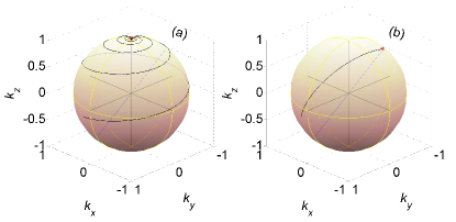
Figure 1: One spin. The black solid line is obtained by numerically integrating of the one-spin modified Schrödinger equation (10). The blue solid (dashed) line connects the origin and the point $\bm{\hat{s}}$ ($-\bm{\hat{s}}$), and $\bm{\omega}$ is parallel to the $\bm{\hat{z}}$ direction. (a) The ratio $\gamma_{\mathrm{D}}/\left|\bm{\omega}\right|=0.25$. The red star symbol represents the analytical approximation for the $\bm{k}$ fixed point given by $\pm\left(\bm{\hat{\omega}}+\left(\gamma_{\mathrm{D}}/\left|\bm{\omega}\right|\right)\left(2\left(1-\bm{\hat{s}}\cdot\bm{\hat{\omega}}\right)\right)^{-1/2}\bm{\hat{s}}\times\bm{\hat{\omega}}\right)$, which is valid when $\gamma_{\mathrm{D}}\ll\left|\bm{\omega}\right|$. (b) The ratio $\gamma_{\mathrm{D}}/\left|\bm{\omega}\right|=25$. The red star symbol represents the analytical approximation for the $\bm{k}$ fixed point given by $-\bm{\hat{s}}+2\left(\left|\bm{\omega}\right|/\gamma_{\mathrm{D}}\right)\bm{\hat{s}}\times\bm{\hat{\omega}}$, which is valid when $\gamma_{\mathrm{D}}\gg\left|\bm{\omega}\right|$.

In the opposite extreme case of $\gamma_{\mathrm{D}}\gg\left|\bm{\omega}\right|$, the dynamics is dominated by the term proportional to $\gamma_{\mathrm{D}}$ in Eq. (10). Note that $\left(\bm{\hat{s}}\cdot\bm{k}\right)\bm{k-\hat{s}}=0$ for $\bm{k}=\pm\bm{\hat{s}}$, and that the term proportional to $\gamma_{\mathrm{D}}$ in Eq. (10) gives rise to attraction (repulsion) of $\bm{k}$ to the point $-\bm{\hat{s}}$ ($+\bm{\hat{s}}$). Consider the case where $\bm{k}=-\bm{\hat{s}}+\bm{\delta}$, and where $\bm{\hat{s}}\cdot\bm{\delta}=0$ ($\bm{\delta}$ is considered as infinitesimally small). To first order in $\left|\bm{\delta}\right|$ Eq. (10) yields

$$\frac{\mathrm{d}\bm{\delta}}{\mathrm{d}t}=2\bm{\omega}\times\left(-\bm{\hat{s}}+\bm{\delta}\right)-\gamma_{\mathrm{D}}\bm{\delta}+O\left(\left|\bm{\delta}\right|^{2}\right)\;.$$ (14)

hence the $\bm{k}$ point $-\bm{\hat{s}}+2\left(\left|\bm{\omega}\right|/\gamma_{\mathrm{D}}\right)\bm{\hat{s}}\times\bm{\hat{\omega}}$ is nearly a stable fixed point when $\gamma_{\mathrm{D}}\gg\left|\bm{\omega}\right|$ [see the red star symbol in Fig. 1(b)].

IV Spin in thermal equilibrium

The effect of coupling between the spin and its environment can be accounted for using the modified Schrödinger equation (1) provided that a fluctuating magnetic field is added Slichter_Principles . Consider the case where the spin Hamiltonian $\mathcal{H}$ is given by $\hbar^{-1}\mathcal{H}=\bm{\omega\cdot\sigma}$, where $\bm{\omega}=\omega_{0}\bm{\hat{z}}+\left(\omega_{x},\omega_{y},\omega_{z}\right)$, where $\omega_{0}$ is a constant, and where $\omega_{x}\left(t\right)$, $\omega_{y}\left(t\right)$ and $\omega_{z}\left(t\right)$ represent the effect of a fluctuating magnetic field. The following is assumed to hold $\left\langle\omega_{x}\right\rangle=\left\langle\omega_{y}\right\rangle=\left\langle\omega_{z}\right\rangle=0$, where $\left\langle{}\right\rangle$ denotes time averaging (i.e. the fluctuating field has a vanishing averaged value), and the correlation function $\left\langle\omega_{i}\left(t\right)\omega_{j}\left(t^{\prime}\right)\right\rangle$ is given by

$$\left\langle\omega_{i}\left(t\right)\omega_{j}\left(t^{\prime}\right)\right\rangle=\delta_{ij}\omega_{\mathrm{s}}^{2}\exp\left(-\frac{\left|t-t^{\prime}\right|}{\tau_{\mathrm{s}}}\right)\;,$$ (15)

where both the variance $\omega_{\mathrm{s}}^{2}$ and the correlation time $\tau_{\mathrm{s}}$ are positive constants, and where $i,j\in\left\{x,y,z\right\}$. The added fluctuating magnetic field gives rise to longitudinal $T_{\mathrm{s}1}^{-1}$ and transverse $T_{\mathrm{s}2}^{-1}$ relaxation rates given by [see Eqs. (17.274) and (17.275) of Ref. Buks_QMLN ]

$$\frac{1}{T_{\mathrm{s}1}}=\frac{2\omega_{\mathrm{s}}^{2}\tau_{\mathrm{s}}}{1+\omega_{0}^{2}\tau_{\mathrm{s}}^{2}}\;,$$ (16)

and

$$\frac{1}{T_{\mathrm{s}2}}=\frac{1}{2T_{\mathrm{s}1}}+\omega_{\mathrm{s}}^{2}\tau_{\mathrm{s}}\;.$$ (17)

The effect of a fluctuating magnetic field is demonstrated by the plot shown in Fig. 2. The time evolution of $\bm{k}$ is evaluated by numerically integrating the modified Schrödinger equation (1) with added fluctuating magnetic field. The parameters used for the calculation are listed in the figure caption. The Wiener-Khinchine theorem is employed to relate the given correlation function (15) to the power spectrum, which, in turn, is used to derive the variance of Fourier coefficients of $\omega_{x}$, $\omega_{y}$ and $\omega_{z}$. The variance values are employed for generating random Fourier coefficients, which in turn, allow generating the functions $\omega_{x}\left(t\right)$, $\omega_{y}\left(t\right)$ and $\omega_{z}\left(t\right)$ in a way consistent with Eq. (15).

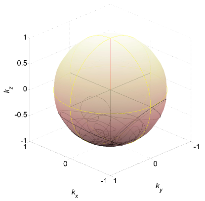
Figure 2: Thermal equilibrium. The red line represents the static magnetic field direction, and the black line the Bloch vector $\bm{k}$. In this calculation $\omega_{0}=10$, $\gamma_{\mathrm{D}}=5$, $\bm{\hat{s}}=\bm{\hat{z}}$, $\omega_{\mathrm{s}}^{2}=10$ and $\tau_{\mathrm{s}}=5$.

To account for the effect of the fluctuating field, a longitudinal relaxation term proportional to $T_{\mathrm{s}1}^{-1}$ is added to Eq. (13). Consider the case where $T_{\mathrm{s}1}^{-1}\ll\gamma_{\mathrm{D}}\ll\left|\bm{\omega}\right|$ and $\bm{\hat{s}}=\bm{\hat{z}}$. For this case Eq. (13) has a steady state solution given by $k_{\parallel}=-1+1/\left(1+2\gamma_{\mathrm{D}}T_{\mathrm{s}1}\right)$ [the term proportional to $s_{x}k_{x}+s_{y}k_{y}$ in Eq. (13) has been disregarded, since it is assumed that $\gamma_{\mathrm{D}}\ll\left|\bm{\omega}\right|$]. The corresponding effective temperature $T_{\mathrm{eff}}$ is given by

$$T_{\mathrm{eff}}=\frac{\hbar\omega_{0}}{2k_{\mathrm{B}}\tanh^{-1}\left(1-\frac{1}{1+2\gamma_{\mathrm{D}}T_{\mathrm{s}1}}\right)}\;,$$ (18)

where $k_{\mathrm{B}}$ is the Boltzmann’s constant.

V Two spins

Consider a two spin 1/2 system in a pure state $\left|\psi\right\rangle$ given by $\left|\psi\right\rangle=a\left|++\right\rangle+b\left|+-\right\rangle+c\left|-+\right\rangle+d\left|--\right\rangle$.

V.1 Single spin angular momentum

The single-spin angular momentum (in units of $\hbar/2$) vector operators are denoted by $\bm{S}_{1}=\left(S_{1x},S_{1y},S_{1z}\right)$ and $\bm{S}_{2}=\left(S_{2x},S_{2y},S_{2z}\right)$, and the total spin angular momentum is $\bm{S}=\bm{S}_{1}+\bm{S}_{2}=\left(S_{x},S_{y},S_{z}\right)$. A given single-spin linear operator of spin 1 (2) is represented by the $4\times 4$ matrix $\sigma_{0}\otimes K$ ($K\otimes\sigma_{0}$) where $\otimes$ denotes the Kronecker tensor product, $\sigma_{0}$ is the $2\times 2$ identity matrix, and where $K$ is the $2\times 2$ matrix representation of the given single-spin operator. The matrix representations of $\bm{S}_{1}\cdot\bm{\hat{u}}_{1}$ and $\bm{S}_{2}\cdot\bm{\hat{u}}_{2}$, where $\bm{\hat{u}}_{1}=\left(\sin\theta_{1}\cos\varphi_{1},\sin\theta_{1}\sin\varphi_{1},\cos\theta_{1}\right)$ and $\bm{\hat{u}}_{2}=\left(\sin\theta_{2}\cos\varphi_{2},\sin\theta_{2}\sin\varphi_{2},\cos\theta_{2}\right)$ are unit vectors, are thus given by [see Eq. (8)]

$$\bm{S}_{1}\cdot\bm{\hat{u}}_{1}$$

$$\dot{=}\left(\begin{array}[c]{cccc}\cos\theta_{1}&0&\sin\theta_{1}e^{-i\varphi_{1}}&0\\ 0&\cos\theta_{1}&0&\sin\theta_{1}e^{-i\varphi_{1}}\\ \sin\theta_{1}e^{i\varphi_{1}}&0&-\cos\theta_{1}&0\\ 0&\sin\theta_{1}e^{i\varphi_{1}}&0&-\cos\theta_{1}\end{array}\right)\;,$$ (23)

and

$$\bm{S}_{2}\cdot\bm{\hat{u}}_{2}$$

$$\dot{=}\left(\begin{array}[c]{cccc}\cos\theta_{2}&\sin\theta_{2}e^{-i\varphi_{2}}&0&0\\ \sin\theta_{2}e^{i\varphi_{2}}&-\cos\theta_{2}&0&0\\ 0&0&\cos\theta_{2}&\sin\theta_{2}e^{-i\varphi_{2}}\\ 0&0&\sin\theta_{2}e^{i\varphi_{2}}&-\cos\theta_{2}\end{array}\right)\;.$$ (29)

With the help of Eqs. (LABEL:S1*u1) and (LABEL:S2*u2) and the normalization condition $aa^{\ast}+bb^{\ast}+cc^{\ast}+dd^{\ast}=1$ one finds that

$$\left|\left\langle\bm{S}_{1}\right\rangle\right|^{2}=\left|\left\langle\bm{S}_{2}\right\rangle\right|^{2}=1-4\left|ad-bc\right|^{2}\;.$$ (31)

Note that the normalization condition implies that $\left|ad-bc\right|^{2}\leq 1/4$. In standard quantum mechanics the term $ad-bc$ is time-independent, provided that the spins are decoupled [see Eq. (8.121) of Ref. Buks_QMLN ]. The term $\left|ad-bc\right|$ can be extracted from the partial transpose $\rho^{\mathrm{T}1}$ ($\rho^{\mathrm{T}2}$) of the spin-spin density operator with respect to spin 1 (2) using the relation $\det\rho^{\mathrm{T}1}=\det\rho^{\mathrm{T}2}=-\left|ad-bc\right|^{4}$ Peres_1413 .

Consider the case where $\left\langle\bm{S}_{1}\right\rangle=\left\langle\bm{S}_{2}\right\rangle=0$. For this case the following holds $\left\langle S_{1z}\right\rangle=a^{\ast}a+b^{\ast}b-c^{\ast}c-d^{\ast}d=0$, $\left\langle S_{2z}\right\rangle=a^{\ast}a-b^{\ast}b+c^{\ast}c-d^{\ast}d=0$, $\left\langle S_{1+}\right\rangle=2\left(a^{\ast}c+b^{\ast}d\right)=0$ and $\left\langle S_{2+}\right\rangle=2\left(a^{\ast}b+c^{\ast}d\right)=0$, where $S_{n\pm}=S_{nx}\pm iS_{ny}$ and $n\in\left\{1,2\right\}$. The conditions $\left\langle S_{1z}\right\rangle=\left\langle S_{2z}\right\rangle=0$ imply that $a^{\ast}a=d^{\ast}d$ and $b^{\ast}b=c^{\ast}c$, whereas the conditions $\left\langle S_{1+}\right\rangle=\left\langle S_{2+}\right\rangle=0$ yield $a^{\ast}/d=-b^{\ast}/c=-c^{\ast}/b$. Hence the state vector $\left|\psi\right\rangle$ for this case has the form

$$\left|\psi\right\rangle =\frac{\cos\frac{\theta_{\psi}}{2}e^{-\frac{i\phi_{\alpha}}{2}}}{\sqrt{2}}\left|++\right\rangle+\frac{\sin\frac{\theta_{\psi}}{2}ie^{-\frac{i\phi_{\beta}}{2}}}{\sqrt{2}}\left|+-\right\rangle$$

$$+\frac{\sin\frac{\theta_{\psi}}{2}ie^{\frac{i\phi_{\beta}}{2}}}{\sqrt{2}}\left|-+\right\rangle+\frac{\cos\frac{\theta_{\psi}}{2}e^{\frac{i\phi_{\alpha}}{2}}}{\sqrt{2}}\left|--\right\rangle\;,$$

(32)

where $\theta_{\psi}$, $\phi_{\alpha}$ and $\phi_{\beta}$ and are real. Note that $ad-bc=1/2$ for the state (32).

The operator $R$ is defined by [note that $\bm{S}_{1}\cdot\bm{S}_{2}=\bm{S}_{2}\cdot\bm{S}_{1}$, see Eqs. (LABEL:S1*u1) and (LABEL:S2*u2)]

$$R=\bm{S}_{1}\cdot\bm{S}_{2}-\left\langle\bm{S}_{1}\right\rangle\cdot\left\langle\bm{S}_{2}\right\rangle\;,$$ (33)

and its expectation value $\left\langle R\right\rangle$ is given by

$$\left\langle R\right\rangle=4\left(\left|ad\right|^{2}-\left|bc\right|^{2}\right)-4\operatorname{Re}\left(\left(b^{\ast}{}^{2}+c^{\ast}{}^{2}\right)\left(ad-bc\right)\right)\;.$$ (34)

Note that $\left\langle R\right\rangle=0$ when $ad-bc=0$.

V.2 Single spin purity

The single-spin purity $P$ is given by $P=1-2\left|ad-bc\right|^{2}$ [see Eq. (8.642) of Ref. Buks_QMLN ]. It is bounded by $1/2\leq P\leq 1$ [recall that $\left|ad-bc\right|^{2}\leq 1/4$]. In terms of the purity $P$, Eq. (31) reads $\left|\left\langle\bm{S}_{1}\right\rangle\right|^{2}=\left|\left\langle\bm{S}_{2}\right\rangle\right|^{2}=2\left(P-1/2\right)$.

V.3 Spin-spin disentanglement

Spin-spin disentanglement is generated by the term proportional to $\gamma_{\mathrm{D}}$ in the modified Schrödinger equation (1) provided that the bra vector $\left\langle\Psi\right|$ is taken to be given by Buks_355303 ; Wootters_2245

$$\left\langle\Psi\right|=d\left\langle++\right|-c\left\langle+-\right|-b\left\langle-+\right|+a\left\langle--\right|\;.$$ (35)

Note that $\left\langle\Psi\right|$ (35) is normalized provided that $\left|\psi\right\rangle$ is normalized, and that $\left\langle\Psi\right.\left|\psi\right\rangle=2\left(ad-bc\right)$ [compare with Eq. (31)].

The plots shown in Fig. 3 are based on numerical integration of the spin-spin modified Schrödinger equation (1) with $\mathcal{H}=0$, and with $\left\langle\Psi\right|$ given by Eq. (35). In the panels labelled by the number ’1’ (’2’), the single-spin purity is initially low $P\simeq 1/2$ (high $P\simeq 1$), i.e. initially$\ \left|ad-bc\right|^{2}\simeq 1/4$ ($\left|ad-bc\right|^{2}\simeq 0$). The three-dimensional plots labelled by the letter ’a’ (’b’) display the time evolution of $\left\langle\bm{S}_{1}\right\rangle$ ($\left\langle\bm{S}_{2}\right\rangle$). In these plots, red straight lines are drawn between the origin and the initial value of $\left\langle\bm{S}_{n}\right\rangle$, whereas green lines represent time evolution of $\left\langle\bm{S}_{n}\right\rangle$, where $n\in\left\{1,2\right\}$. The plots labelled by the letters ’c’ and ’d’ display the time evolution of $P$ and $\left\langle R\right\rangle$ [see Eq. (33)], respectively. For both cases ’1’ and ’2’, $\left|\left\langle\bm{S}_{1}\right\rangle\right|^{2}=\left|\left\langle\bm{S}_{2}\right\rangle\right|^{2}\rightarrow 1$ [i.e. $\left|ad-bc\right|^{2}\rightarrow 0$ and $P\rightarrow 1$, see Eq. (31)] in the long time limit $t\rightarrow\infty$, i.e. entanglement vanishes in this limit.

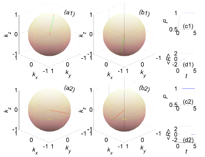
Figure 3: Spin-spin disentanglement. In the panels labelled by the numbers ’1’ (’2’), the single-spin purity is initially $P\simeq 1/2$ ($P\simeq 1$). The (initial value) time evolution of $\left\langle\bm{S}_{1}\right\rangle$ and $\left\langle\bm{S}_{2}\right\rangle$ is indicated by red (green) lines in the plots labelled by the letter ’a’ and ’b’, respectively. The single spin purity $P$ and $\left\langle R\right\rangle$ are shown as a function of time $t$ in the plots labelled by the letters ’c’ and ’d’, respectively.

The case where initially $P\simeq 1/2$ [see Fig. 3 (a1), (b1), (c1) and (d1)] is explored by numerically integrating the modified Schrödinger equation (1) with the initial condition (before normalization) of $\left|\psi\right\rangle=\left|\psi_{0}\right\rangle+\epsilon\left|\psi_{\mathrm{p}}\right\rangle$, where $\left|\psi_{0}\right\rangle=\left|\mathrm{B}_{0,0}\right\rangle=2^{-1/2}\left(\left|+-\right\rangle-\left|-+\right\rangle\right)$ is the singlet Bell state (which is invariant under single-spin basis transformation, and which is fully entangled), $\epsilon$ is a small positive number, and $\left|\psi_{\mathrm{p}}\right\rangle=\alpha\left|++\right\rangle+\beta\left|+-\right\rangle+\gamma\left|-+\right\rangle+\delta\left|--\right\rangle$ is normalized. For this case, to first order in $\epsilon$ initially $\left\langle S_{1+}\right\rangle=-\left\langle S_{2+}\right\rangle=2^{1/2}\left(\delta-\alpha^{\ast}\right)\epsilon$ and $\left\langle S_{1z}\right\rangle=-\left\langle S_{2z}\right\rangle=2^{-1/2}\left(\beta+\beta^{\ast}+\gamma+\gamma^{\ast}\right)\epsilon$, i.e. initially $\left\langle\bm{S}_{1}\right\rangle=-\left\langle\bm{S}_{2}\right\rangle$. The plots in Fig. 3 (a1), (b1), (c1) and (d1) demonstrate that both $\left\langle\bm{S}_{1}\right\rangle$ and $\left\langle\bm{S}_{2}\right\rangle$ increase in magnitude with time while remaining nearly anti-parallel to each other as they both approach the Bloch sphere surfaces. The red star symbols in Fig. 3(a1) and (b1) indicate the initial values of $\left\langle\bm{S}_{1}\right\rangle/\left|\left\langle\bm{S}_{1}\right\rangle\right|$ and $\left\langle\bm{S}_{2}\right\rangle/\left|\left\langle\bm{S}_{2}\right\rangle\right|$. As the plots in Fig. 3(a1) and (b1) demonstrate, time evolution leaves these normalized values nearly unchanged, provided that $\epsilon\ll 1$ (the value of $\epsilon=0.1$ has been used for generating the plots).

The case shown in Fig. 3 (a1), (b1), (c1) and (d1) demonstrates strong dependency of the long time value of $\left|\psi\right\rangle$ on its initial value. This dependency, which becomes extreme when $\left|\psi\right\rangle$ is initially fully entangled, resembles the butterfly effect. In the limit $\epsilon\rightarrow 0$, angular momentum is conserved by the modified Schrödinger equation, provided that $\left|\psi_{0}\right\rangle=\left|\mathrm{B}_{0,0}\right\rangle$. This can be attributed to the fact that $S_{x}\left|\mathrm{B}_{0,0}\right\rangle=S_{y}\left|\mathrm{B}_{0,0}\right\rangle=S_{z}\left|\mathrm{B}_{0,0}\right\rangle=0$. Conservation of the angular momentum $\bm{\hat{z}}$ component is obtained when the initial state is the Bell triplet state $\left|\mathrm{B}_{1,0}\right\rangle=2^{-1/2}\left(\left|+-\right\rangle+\left|-+\right\rangle\right)$, which is also fully entangled, and for which $S_{z}\left|\mathrm{B}_{1,0}\right\rangle=0$.

The case where initially $P\simeq 1$ is demonstrated by Fig. 3 (a2), (b2), (c2) and (d2). For this case both $\left\langle\bm{S}_{1}\right\rangle$ and $\left\langle\bm{S}_{2}\right\rangle$ are initially close to the Bloch sphere surfaces. Consequently, the time evolution of $\left|\psi\right\rangle$ towards a fully product state does not significantly change $\left\langle\bm{S}_{1}\right\rangle$ and $\left\langle\bm{S}_{2}\right\rangle$ (time evolution is represented by the green lines).

VI Instability

Consider a system composed of two spins 1/2. The first spin, which is labelled as ’$\mathrm{a}$’, has a relatively low angular frequency $\omega_{\mathrm{a}}$ in comparison with the angular frequency $\omega_{\mathrm{b}}$ of the second spin, which is labelled as ’$\mathrm{b}$’, and which is externally driven. The angular momentum vector operator of particle $\mathrm{a}$ ($\mathrm{b}$) is denoted by $\bm{S}_{\mathrm{a}}$ ($\bm{S}_{\mathrm{b}}$). The Hamiltonian $\mathcal{H}$ of the closed system is given by

$$\mathcal{H}=\omega_{\mathrm{a}}S_{\mathrm{az}}+\omega_{\mathrm{b}}S_{\mathrm{bz}}+\frac{\omega_{1}\left(S_{\mathrm{b+}}+S_{\mathrm{b-}}\right)}{2}+V\;,$$ (36)

where the driving amplitude and angular frequency are denoted by $\omega_{1}$ and $-\omega_{\mathrm{p}}=\omega_{\mathrm{b}}-\Delta$, respectively ($-\Delta$ is the driving detuning), the operators $S_{\mathrm{a\pm}}$ are given by $S_{\mathrm{a\pm}}=S_{\mathrm{ax}}\pm iS_{\mathrm{ay}}$, and the rotated operators $S_{\mathrm{b\pm}}$ are given by $S_{\mathrm{b\pm}}=\left(S_{\mathrm{bx}}\pm iS_{\mathrm{by}}\right)e^{\mp i\omega_{\mathrm{p}}t}$. The coupling term is given by $V=g\hbar^{-1}\left(S_{\mathrm{a+}}+S_{\mathrm{a-}}\right)S_{\mathrm{bz}}$, where $g$ is a coupling rate. In a rotating frame, the matrix representation of the transformed Hamiltonian $\mathcal{H}^{\prime}$ is given by $\mathcal{H}^{\prime}\dot{=}\hbar\Omega$, where the $4\times 4$ matrix $\Omega$ is given by

$$\Omega=\left(\begin{array}[c]{cccc}\frac{\omega_{\mathrm{a}}+\Delta}{2}&\frac{\omega_{1}}{2}&\frac{g}{2}&0\\ \frac{\omega_{1}}{2}&\frac{\omega_{\mathrm{a}}-\Delta}{2}&0&-\frac{g}{2}\\ \frac{g}{2}&0&\frac{-\omega_{\mathrm{a}}+\Delta}{2}&\frac{\omega_{1}}{2}\\ 0&-\frac{g}{2}&\frac{\omega_{1}}{2}&\frac{-\omega_{\mathrm{a}}-\Delta}{2}\end{array}\right)\;.$$ (37)

Disentanglement is generated by the modified Schrödinger equation (1) by choosing the bra vector $\left\langle\Psi\right|$ to be given by Eq. (35). The expectation values of $\left\langle\bm{S}_{1}\right\rangle$ and $\left\langle\bm{S}_{2}\right\rangle$, which are shown in Fig. 4(a) and in Fig. 4(b), respectively, are calculated by numerically integrating the modified Schrödinger equation (1). For the plot shown in Fig. 4, for which the Hartmann–Hahn matching condition $\omega_{\mathrm{a}}=\omega_{\mathrm{R}}$ Hartmann1962 ; Yang_1 ; Levi_053516  is assumed to be satisfied, where $\omega_{\mathrm{R}}=\sqrt{\omega_{1}^{2}+\Delta^{2}}$ is the Rabi angular frequency, both $\left\langle\bm{S}_{1}\right\rangle$ and $\left\langle\bm{S}_{2}\right\rangle$ undergo a limit cycle (LC). The instability responsible for the LC was studied in Ref. Levi_053516 , in which the equations of motion generated by the Hamiltonian (36) were treated using in the mean-field approximation. This example demonstrates the connection between the mean-field approximation and disentanglement.

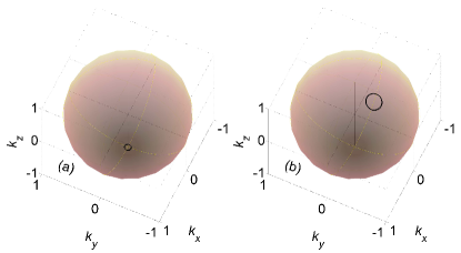
Figure 4: Dipolar LC. The expectation values of $\left\langle\bm{S}_{1}\right\rangle$ and $\left\langle\bm{S}_{2}\right\rangle$ are shown in (a) and (b), respectively. The modified Schrödinger equation (1), with the Hamiltonian (36) and the bra vector (35) is numerically integrated. The parameters used for the calculation are $\gamma_{\mathrm{D}}=10^{3}$, $\omega_{\mathrm{a}}=10^{2}$, $\omega_{1}=-\Delta=2^{-1/2}\omega_{\mathrm{a}}$ and $g=0.2$. Fluctuating magnetic field with parameters $\omega_{\mathrm{s}}^{2}=1$ and $\tau_{\mathrm{s}}=0.05$ is added [see Eq. (15)].

VII Summary

In summary, both processes of thermalization and disentanglement can be modeled using a recently proposed modified Schrödinger equation. The added nonlinear term can give rise to instabilities and LC solutions. On the other hand, it remains unclear whether quantum mechanics can be self-consistently reformulated based on the proposed modified Schrödinger equation. Future study will be devoted to exploring candidate formalisms.

VIII Acknowledgments

This work was supported by the Israeli science foundation, the Israeli ministry of science, and by the Technion security research foundation. We thank Michael R. Geller for helpful discussions.

References

- (1) E. Schrodinger, “Die gegenwartige situation in der quantenmechanik”, Naturwissenschaften, vol. 23, pp. 807, 1935.
- (2) Roger Penrose, “Uncertainty in quantum mechanics: faith or fantasy?”, Philosophical Transactions of the Royal Society A: Mathematical, Physical and Engineering Sciences, vol. 369, no. 1956, pp. 4864–4890, 2011.
- (3) A. J. Leggett, “Experimental approaches to the quantum measurement paradox”, Found. Phys., vol. 18, pp. 939–952, 1988.
- (4) A. J. Leggett, “Realism and the physical world”, Rep. Prog. Phys., vol. 71, pp. 022001, 2008.
- (5) Michael R Geller, “Fast quantum state discrimination with nonlinear ptp channels”, arXiv:2111.05977, 2021.
- (6) Steven Weinberg, “Testing quantum mechanics”, Annals of Physics, vol. 194, no. 2, pp. 336–386, 1989.
- (7) Steven Weinberg, “Precision tests of quantum mechanics”, in THE OSKAR KLEIN MEMORIAL LECTURES 1988–1999, pp. 61–68. World Scientific, 2014.
- (8) H-D Doebner and Gerald A Goldin, “On a general nonlinear schrödinger equation admitting diffusion currents”, Physics Letters A, vol. 162, no. 5, pp. 397–401, 1992.
- (9) H-D Doebner and Gerald A Goldin, “Introducing nonlinear gauge transformations in a family of nonlinear schrödinger equations”, Physical Review A, vol. 54, no. 5, pp. 3764, 1996.
- (10) Nicolas Gisin and Ian C Percival, “The quantum-state diffusion model applied to open systems”, Journal of Physics A: Mathematical and General, vol. 25, no. 21, pp. 5677, 1992.
- (11) David E Kaplan and Surjeet Rajendran, “Causal framework for nonlinear quantum mechanics”, Physical Review D, vol. 105, no. 5, pp. 055002, 2022.
- (12) Manuel H Muñoz-Arias, Pablo M Poggi, Poul S Jessen, and Ivan H Deutsch, “Simulating nonlinear dynamics of collective spins via quantum measurement and feedback”, Physical review letters, vol. 124, no. 11, pp. 110503, 2020.
- (13) Angelo Bassi, Kinjalk Lochan, Seema Satin, Tejinder P Singh, and Hendrik Ulbricht, “Models of wave-function collapse, underlying theories, and experimental tests”, Reviews of Modern Physics, vol. 85, no. 2, pp. 471, 2013.
- (14) Eyal Buks, “Disentanglement and a nonlinear schrödinger equation”, Journal of Physics A: Mathematical and Theoretical, vol. 55, no. 35, pp. 355303, 2022.
- (15) Lajos Diósi, “Stochastic pure state representation for open quantum systems”, Physics Letters A, vol. 114, no. 8-9, pp. 451–454, 1986.
- (16) Klaus Mølmer, Yvan Castin, and Jean Dalibard, “Monte carlo wave-function method in quantum optics”, JOSA B, vol. 10, no. 3, pp. 524–538, 1993.
- (17) Jean Dalibard, Yvan Castin, and Klaus Mølmer, “Wave-function approach to dissipative processes in quantum optics”, Physical review letters, vol. 68, no. 5, pp. 580, 1992.
- (18) V Semin, I Semina, and F Petruccione, “Stochastic wave-function unravelling of the generalized lindblad equation”, Physical Review E, vol. 96, no. 6, pp. 063313, 2017.
- (19) Roei Levi, Sergei Masis, and Eyal Buks, “Instability in the hartmann-hahn double resonance”, Phys. Rev. A, vol. 102, pp. 053516, Nov 2020.
- (20) Heinz-Peter Breuer, Francesco Petruccione, et al., The theory of open quantum systems, Oxford University Press on Demand, 2002.
- (21) Barbara Drossel, “What condensed matter physics and statistical physics teach us about the limits of unitary time evolution”, Quantum Studies: Mathematics and Foundations, vol. 7, no. 2, pp. 217–231, 2020.
- (22) C Hicke and MI Dykman, “Classical dynamics of resonantly modulated large-spin systems”, Physical Review B, vol. 78, no. 2, pp. 024401, 2008.
- (23) Waldemar Kłobus, Paweł Kurzyński, Marek Kuś, Wiesław Laskowski, Robert Przybycień, and Karol Życzkowski, “Transition from order to chaos in reduced quantum dynamics”, Physical Review E, vol. 105, no. 3, pp. 034201, 2022.
- (24) Krzysztof Kowalski, “Linear and integrable nonlinear evolution of the qutrit”, Quantum Information Processing, vol. 19, no. 5, pp. 1–31, 2020.
- (25) Bernd Fernengel and Barbara Drossel, “Bifurcations and chaos in nonlinear lindblad equations”, Journal of Physics A: Mathematical and Theoretical, vol. 53, no. 38, pp. 385701, 2020.
- (26) K Kowalski and J Rembieliński, “Integrable nonlinear evolution of the qubit”, Annals of Physics, vol. 411, pp. 167955, 2019.
- (27) Charles P Slichter, Principles of magnetic resonance, vol. 1, Springer Science & Business Media, 2013.
- (28) Eyal Buks, Quantum mechanics - Lecture Notes, http://buks.net.technion.ac.il/teaching/, 2020.
- (29) Asher Peres, “Separability criterion for density matrices”, Physical Review Letters, vol. 77, no. 8, pp. 1413, 1996.
- (30) William K Wootters, “Entanglement of formation of an arbitrary state of two qubits”, Physical Review Letters, vol. 80, no. 10, pp. 2245, 1998.
- (31) SR Hartmann and EL Hahn, “Nuclear double resonance in the rotating frame”, Physical Review, vol. 128, no. 5, pp. 2042, 1962.
- (32) Pengcheng Yang, Martin B Plenio, and Jianming Cai, “Dynamical nuclear polarization using multi-colour control of color centers in diamond”, EPJ Quantum Technology, vol. 3, pp. 1–9, 2016.