Dimensionality-Varying Diffusion Process

Abstract

Diffusion models, which learn to reverse a signal destruction process to generate new data, typically require the signal at each step to have the same dimension. We argue that, considering the spatial redundancy in image signals, there is no need to maintain a high dimensionality in the evolution process, especially in the early generation phase. To this end, we make a theoretical generalization of the forward diffusion process via signal decomposition. Concretely, we manage to decompose an image into multiple orthogonal components and control the attenuation of each component when perturbing the image. That way, along with the noise strength increasing, we are able to diminish those inconsequential components and thus use a lower-dimensional signal to represent the source, barely losing information. Such a reformulation allows to vary dimensions in both training and inference of diffusion models. Extensive experiments on a range of datasets suggest that our approach substantially reduces the computational cost and achieves on-par or even better synthesis performance compared to baseline methods. We also show that our strategy facilitates high-resolution image synthesis and improves FID of diffusion model trained on FFHQ at $1024\times 1024$ resolution from 52.40 to 10.46. Code and models will be made publicly available.

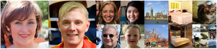
Fig. 1: Synthesized samples on various datasets, including FFHQ ($1024^{2}$ and $256^{2}$), LSUN Church ($256^{2}$), LSUN Bedroom ($256^{2}$), LSUN Cat 256 ($256^{2}$) and CIFAR10 ($32^{2}$). All these samples are generated from a $64^{2}$ noise except CIFAR10 from $16^{2}$, while conventional diffusion models can only start from a noise with the same dimension as the final sample.

1 Introduction

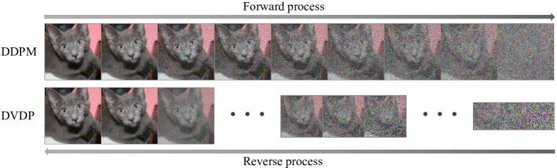
Fig. 2: Conceptual comparison between DDPM [6] and our proposed DVDP, where our approach allows using a varying dimension in the diffusion process.

Diffusion models [6, 26, 2, 19, 22] have recently shown great potential in image synthesis. Instead of directly learning the observed distribution, it constructs a multi-step forward process through gradually adding noise onto the real data (i.e., diffusion). After a sufficiently large number of steps, the source signal could be considered as completely destroyed, resulting in a pure noise distribution that naturally supports sampling. In this way, starting from sampled noises, we can expect new instances after reversing the diffusion process step by step.

As it can be seen, the above pipeline does not change the dimension of the source signal throughout the entire diffusion process [24, 6, 26]. It thus requires the reverse process to map a high-dimensional input to a high-dimensional output at every single step, causing heavy computation overheads [20, 9]. However, images present a measure of spatial redundancy [4] from the semantic perspective (e.g., an image pixel could usually be easily predicted according to its neighbours). Given such a fact, when the source signal is attenuated to some extent along with the noise strength growing, it should be possible to get replaced by a lower-dimensional signal. We therefore argue that there is no need to follow the source signal dimension along the entire distribution evolution process, especially at early steps (i.e., steps close to the pure noise distribution) for coarse generation.

In this work, we propose dimensionality-varying diffusion process (DVDP), which allows dynamically adjusting the signal dimension when constructing the forward path. For this purpose, we first decompose an image into multiple orthogonal components, each of which owns dimension lower than the original data. Then, based on such a decomposition, we theoretically generalize the conventional diffusion process such that we can control the attenuation of each component when adding noise. Thanks to this reformulation, we manage to drop those inconsequential components after the noise strength reaches a certain level, and thus represent the source image using a lower-dimensional signal with little information lost. The remaining diffusion process could inherit this dimension and apply the same technique to further reduce the dimension.

We evaluate our approach on various datasets, including objects, human faces, animals, indoor scenes, and outdoor scenes. Experimental results suggest that DVDP achieves on-par or even better synthesis performance than baseline models on all datasets. More importantly, DVDP relies on much fewer computations, and hence speeds up both training and inference of diffusion models. We also demonstrate the effectiveness of our approach in learning from high-resolution data. For example, we are able to start from a $64\times 64$ noise to produce an image under $1024\times 1024$ resolution. With FID [5] as the evaluation metric, our $1024\times 1024$ model trained on FFHQ improves the baseline [26] from 52.40 to 10.46. All these advantages benefit from using a lower-dimensional signal, which reduces the computational cost and mitigates the optimization difficulty.

2 Related Work

Diffusion models. Sohl-Dickstein et al. [24] propose diffusion models for the first time that generate samples from a target distribution by reversing a diffusion process in which target distribution is gradually disturbed to an easily sampled standard Gaussian. Ho et al. [6] further propose DDPM to reverse the diffusion process by learning a noise prediction network. Song et al. [26] consider diffusion models as stochastic differential equations with continuous timesteps and proposes a unified framework.

Accelerating diffusion models. Diffusion models significantly suffer from the slow training and inference speed. There are many methods that speed up sampling from thousands of steps to tens of steps while keeping an acceptable sample quality [1, 15, 25, 17, 28, 29, 23, 13]. Besides improvements only on inference speed, there are other works aiming at speeding up both training and inference. Luhman et al. [16] propose a patch operation to decrease the dimensionality of each channel while accordingly increasing the number of channels, which greatly reduces the complexity of computation. Besides, a trainable forward process [31] is also proven to benefit a faster training and inference speed. However, the price of their acceleration is a poor sampling quality evaluated by FID score. In this work, we accelerate DDPM on both training and inference from a different perspective by heavily reducing the dimensionality of the early diffusion process and thus improving the efficiency while obtaining on-par or even better quality of generation.

Varying dimensionality of diffusion models. Due to the redundancy in image signals, it is possible to improve the efficiency of diffusion models by varying dimensionality during the generation process. The most relevant work to our proposed model is subspace diffusion [9], which can also vary dimensionality in the diffusion process. However, subspace diffusion suffers from a trade-off between sampling acceleration and sample quality as claimed in [9], while our DVDP can relieve this dilemma (see theoretical analysis in Sec. 4.4 and experimental results in Sec. 5.3). Instead of varying dimensionality in one diffusion process, there are works cascading several diffusion processes with growing dimensionality [7, 19, 22, 21], where the subsequent process is conditioned on the previous samples.

Discussion with latent diffusion. Besides varying dimensionality in image space, there are other methods, which we generally call latent diffusion, that directly apply diffusion models in a low dimensional latent space, obtained by an autoencoder [8, 20, 3, 27, 18]. Although latent diffusion can also speed up the training and sampling of diffusion models, it decreases dimensionality by an additional model and keeps the diffusion process unchanged. In this paper, however, we focus on the improvement on the diffusion process itself to accelerate training and sampling, which is totally a different route. Besides training and sampling efficiency, another important contribution of this work is to prove that it it unnecessary for diffusion process to keep a fixed dimension along time. By controlling the attenuation of each data component, it is possible to change dimensionality while keeping the process reversible. Thus, we will not further compare our DVDP with latent diffusion.

3 Background

We first introduce the background of Denoising Diffusion Probabilistic Model (DDPM) [24, 6] and some of its extensions which are closely related to our work. DDPM constructs a forward process to perturb the distribution of data $q({\mathbf{x}}_{0})$ into a standard Gaussian ${\mathcal{N}}(\mathbf{0};{\bm{I}})$. Considering an increasing variance schedule of noises $\beta_{1},\dots,\beta_{T}$, DDPMs define the forward process as a Markov chain

$$\vspace{-5pt}{\mathbf{x}}_{t}=\sqrt{1-\beta_{t}}{\mathbf{x}}_{t-1}+\sqrt{\beta_{t}}{\mathbf{\epsilon}},~{}t=1,2,\cdots,T,$$ (1)

where ${\mathbf{\epsilon}}$ is a standard Gaussian noise. In order to generate high-fidelity images, DDPM [6] denoises samples from a standard Gaussian iteratively utilizing the reverse process parameterized as

$$\vspace{-5pt}{\mathbf{x}}_{t-1}=\frac{1}{\sqrt{\alpha_{t}}}\left({\mathbf{x}}_{t}-\frac{\beta_{t}}{\sqrt{1-\bar{\alpha}_{t}}}\epsilon_{\theta}({\mathbf{x}}_{t},t)\right)+\sqrt{\beta_{t}}{\mathbf{\epsilon}},$$ (2)

where $\alpha_{t}=1-\beta_{t},~{}\bar{\alpha}_{t}=\prod_{s=1}^{t}\alpha_{s}$, and ${\mathbf{\epsilon}}_{\theta}$ is a neural network used to predict ${\mathbf{\epsilon}}$ from ${\mathbf{x}}_{t}$. The parameters $\theta$ are learned by minimizing the following loss function

$$\vspace{-5pt}L(\theta)=\mathbb{E}_{t,{\mathbf{x}}_{0},{\mathbf{\epsilon}}}\left[\left\|{\mathbf{\epsilon}}-{\mathbf{\epsilon}}_{\theta}({\mathbf{x}}_{t}({\mathbf{x}}_{0},{\mathbf{\epsilon}}),t)\right\|^{2}\right].$$ (3)

The standard diffusion model is implemented directly in the image space, which is probably not the optimal choice according to [12], and the relative importance of different frequency components can be taken into consideration. [12] implements the diffusion models in a designed space by generalizing diffusion process with the forward process formulated as

$$\vspace{-5pt}{\mathbf{x}}_{t}={\bm{U}}({\bm{I}}-{\bm{B}}_{t})^{\frac{1}{2}}{\bm{U}}^{T}{\mathbf{x}}_{t-1}+{\bm{U}}{\bm{B}}_{t}{\bm{U}}^{T}{\mathbf{\epsilon}},$$ (4)

where ${\bm{U}}$ is an orthogonal matrix to impose a rotation on ${\mathbf{x}}_{t}$, and the noise schedule is defined by the diagonal matrix $\mathbf{B}_{t}$. In this work, we extend the aforementioned generalized framework further and make it possible to vary dimensionality during the diffusion process.

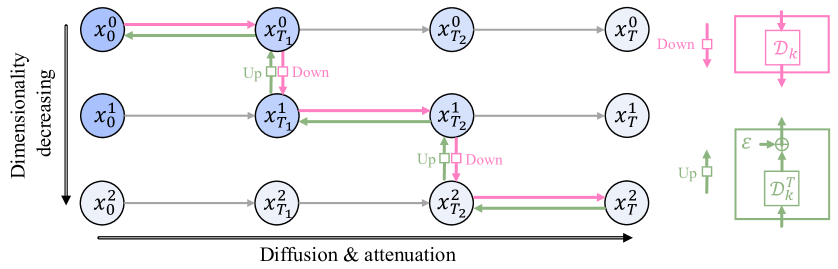
Fig. 3: Framework illustration of DVDP. Each row represents an Attenuated Diffusion Process (ADP), which controls the attenuation of each data component while adding noise. All $K+1$ ADPs ($K=2$ here) have different dimensionality decreasing from top to bottom, and are concatenated by some simple opeartions to obtain our DVDP. In the forward process, the concatenation is achieved by downsampling operation, and in reverse process, it is the upsampling operation followed by adding a Gaussian noise.

4 Dimensionality-Varying Diffusion Process

We formulate the dimensionality-varying diffusion process (DVDP) in this section, which progressively decreases the dimension of ${\mathbf{x}}_{t}$ in forward process, and can be effectively reversed to generate high-dimensional data from a low-dimensional noise. To establish DVDP, we gradually attenuate components of ${\mathbf{x}}_{0}$ in different subspaces and decrease the dimensionality of ${\mathbf{x}}_{t}$ at dimensionality turning points by downsampling operator (Sec. 4.1), which is approximately reversible (Sec. 4.2) with controllable small error caused by the loss of attenuated ${\mathbf{x}}_{0}$ component (Sec. 4.3).

4.1 Forward Process of DVDP

In this section, we will construct the forward process of our DVDP, which decreases the dimensionality as time evolves and can be effectively reversed. To this end, we concatenate multiple diffusion processes with different dimensions into an entire Markov chain by downsampling operations, while we elaborately design each process so that the information loss induced by downsampling is negligible. Fig. 3 illustrates this overall framework. The concatenation of different processes enables us to decrease the dimensionality, and the control on information loss ensures that downsampling operations are approximately reversible, such that the entire process can be reversed (discussed later in Sec. 4.2).

To limit the information loss, we decompose the data into orthogonal components and control the attenuation of each component in the forward process of each concatenated diffusion, which we call Attenuated Diffusion Process (ADP). Once the lost data component induced by downsampling is small enough, the information loss will be negligible. In the following part of this section, we will first introduce the design of each ADP. Then we will show how to merge these ADPs to obtain our DVDP.

Notation list. We first define a sequence of subspaces and other necessary notations as follows:

• ${\mathbb{S}}_{0}\supsetneq{\mathbb{S}}_{1}\supsetneq\cdots\supsetneq{\mathbb{S}}_{K}$ is a sequence of subspaces with decreasing dimensionality $d=\bar{d}_{0}>\bar{d}_{1}>\cdots>\bar{d}_{K}$, where ${\mathbb{S}}_{0}={\mathbb{R}}^{d}$ is the original space, $K\in{\mathbb{N}}_{+}$. For simplicity, ${\mathbb{S}}_{K+1}\triangleq\{{\bm{0}}\}$ and $\bar{d}_{K+1}\triangleq 0$.

• $d_{i}={\rm dim}({\mathbb{S}}_{i}/{\mathbb{S}}_{i+1}),~{}i=0,1,\cdots,K$. Note that $d_{K}={\rm dim}({\mathbb{S}}_{K}/{\mathbb{S}}_{K+1})={\rm dim}({\mathbb{S}}_{K})$.

• $\hat{{\bm{U}}}_{i}\in{\mathbb{R}}^{d\times d_{i}}$ is a matrix whose columns span subspace ${\mathbb{S}}_{i}/{\mathbb{S}}_{i+1}$ for $i=0,1,\cdots,K$.

• ${\bm{U}}_{0}=[\hat{{\bm{U}}}_{0},\cdots,\hat{{\bm{U}}}_{K}]\in{\mathbb{R}}^{d\times d}$ is an orthogonal matrix.

• ${\bm{U}}_{k}\in{\mathbb{R}}^{\bar{d}_{k}\times\bar{d}_{k}}$ is orthogonal matrix, $k=1,2,\cdots,K$.

• ${\bm{U}}_{k}=[{\bm{N}}_{k},{\bm{B}}_{k}]$ splits each ${\bm{U}}_{k}$ into two sub-matrices, where ${\bm{N}}_{k}\in{\mathbb{R}}^{\bar{d}_{k}\times d_{k}}$, ${\bm{B}}_{k}\in{\mathbb{R}}^{\bar{d}_{k}\times\bar{d}_{k+1}}$, $k=0,1,\cdots,K$.

• ${\bm{I}}_{n}\in{\mathbb{R}}^{n\times n}$ is an identity matrix.

• ${\bm{O}}_{n}\in{\mathbb{R}}^{n\times n}$ is a zero matrix.

With the above definitions, we can first construct an ADP ${\mathbf{x}}_{t}^{0},~{}t=0,1,\cdots,T$ in ${\mathbb{S}}_{0}$ as

$${\mathbf{x}}_{t}^{0}= \sum_{i=0}^{K}(\bar{\lambda}_{i,t}{\mathbf{v}}_{i}^{0}+\bar{\sigma}_{i,t}{\mathbf{z}}_{i}^{0})$$ (5)

$$= {\bm{U}}_{0}\bar{{\bm{\Lambda}}}_{0,t}{\bm{U}}_{0}^{T}{\mathbf{x}}_{0}^{0}+{\bm{U}}_{0}\bar{{\bm{L}}}_{0,t}{\bm{U}}_{0}^{T}{\mathbf{\epsilon}}^{0},$$

where ${\mathbf{v}}_{i}^{0}\in{\mathbb{S}}_{i}/{\mathbb{S}}_{i+1}$ is the component of original data point ${\mathbf{x}}_{0}^{0}$ in subspace ${\mathbb{S}}_{i}/{\mathbb{S}}_{i+1}$, $\bar{\lambda}_{i,t}$ controls the attenuation of ${\mathbf{v}}_{i}^{0}$ along timestep $t$, ${\mathbf{z}}_{i}^{0}$ is the component of a standard Gaussian noise ${\mathbf{\epsilon}}^{0}\in{\mathbb{R}}^{\bar{d}_{0}}$ in the same subspace as ${\mathbf{v}}_{i}^{0}$ (i.e., ${\mathbb{S}}_{i}/{\mathbb{S}}_{i+1}$), $\bar{\sigma}_{i,t}$ is the standard deviation of ${\mathbf{z}}_{i}^{0}$, and $\bar{{\bm{\Lambda}}}_{0,t},~{}\bar{{\bm{L}}}_{0,t}\in{\mathbb{R}}^{\bar{d}_{0}\times\bar{d}_{0}}$ are two diagonal matrices defined as $\bar{{\bm{\Lambda}}}_{0,t}={\rm diag}(\bar{\lambda}_{0,t}{\bm{I}}_{d_{0}},~{}\bar{\lambda}_{1,t}{\bm{I}}_{d_{1}},~{}\cdots,~{}\bar{\lambda}_{K,t}{\bm{I}}_{d_{K}})$, $\bar{{\bm{L}}}_{0,t}={\rm diag}(\bar{\sigma}_{0,t}{\bm{I}}_{d_{0}},~{}\bar{\sigma}_{1,t}{\bm{I}}_{d_{1}},~{}\cdots,~{}\bar{\sigma}_{K,t}{\bm{I}}_{d_{K}})$. For compatibility at $t=0$, we have $\bar{{\bm{\Lambda}}}_{0,0}={\bm{I}}_{\bar{d}_{0}}$ and $\bar{{\bm{L}}}_{0,0}={\bm{O}}_{\bar{d}_{0}}$, i.e., $\bar{\lambda}_{i,0}=1$ and $\bar{\sigma}_{i,0}=0$ for all $i=0,1,\cdots,K$. To control the attenuation of each data component ${\mathbf{v}}_{i}^{0}$, we require $\bar{\lambda}_{i,t}$ to gradually decrease from 1 to approximate 0 for $i=0,1,\cdots,K-1$ as timestep $t$ evolves. As for $\bar{\lambda}_{K,t}$, it is not required to decrease (explained later after LABEL:eq:dvdp-chain).

Starting from ${\mathbf{x}}_{t}^{0}$, we can recursively construct a dimensionality-decreasing sequence of ADPs

$${\mathbf{x}}_{t}^{k} ={\mathcal{D}}_{k}{\mathbf{x}}_{t}^{k-1}=\sum_{i=k}^{K}(\bar{\lambda}_{i,t}{\mathbf{v}}_{i}^{k}+\bar{\sigma}_{i,t}{\mathbf{z}}_{i}^{k})$$ (6)

$$={\bm{U}}_{k}\bar{{\bm{\Lambda}}}_{k,t}{\bm{U}}_{k}^{T}{\mathbf{x}}_{0}^{k}+{\bm{U}}_{k}\bar{{\bm{L}}}_{k,t}{\bm{U}}_{k}^{T}{\mathbf{\epsilon}}^{k},~{}1\leq k\leq K,$$

where ${\mathcal{D}}_{k}:{\mathbb{R}}^{\bar{d}_{k-1}}\rightarrow{\mathbb{R}}^{\bar{d}_{k}}$ is a linear surjection, which we call the $k$-th downsampling operator as it reduces the dimensionality of the operand (without ambiguity, we also use ${\mathcal{D}}_{k}$ to denote the corresponding matrix in ${\mathbb{R}}^{\bar{d}_{k}\times\bar{d}_{k-1}}$), ${\mathbf{v}}_{i}^{k}={\mathcal{D}}_{k}{\mathbf{v}}_{i}^{k-1}\in\overline{{\mathcal{D}}}_{k}({\mathbb{S}}_{i}/{\mathbb{S}}_{i+1})$ is the component of ${\mathbf{x}}_{0}^{k}={\mathcal{D}}_{k}{\mathbf{x}}_{o}^{k-1}\in{\mathbb{R}}^{\bar{d}_{k}}$ ($\overline{{\mathcal{D}}}_{k}\triangleq\prod_{i=1}^{k}{\mathcal{D}}_{i}$), ${\mathbf{z}}_{i}^{k}={\mathcal{D}}_{k}{\mathbf{z}}_{i}^{k-1}\in\overline{{\mathcal{D}}}_{k}({\mathbb{S}}_{i}/{\mathbb{S}}_{i+1})$ is the component of a standard Gaussian noise ${\mathbf{\epsilon}}^{k}={\mathcal{D}}_{k}{\mathbf{\epsilon}}^{k-1}\in{\mathbb{R}}^{\bar{d}_{k}}$, $\bar{{\bm{\Lambda}}}_{k,t}={\rm diag}(\bar{\lambda}_{k,t}{\bm{I}}_{d_{k}},~{}\bar{\lambda}_{k+1,t}{\bm{I}}_{d_{k+1}},~{}\cdots,~{}\bar{\lambda}_{K,t}{\bm{I}}_{d_{K}})\in{\mathbb{R}}^{\bar{d}_{k}\times\bar{d}_{k}}$, $\bar{{\bm{L}}}_{k,t}={\rm diag}(\bar{\sigma}_{k,t}{\bm{I}}_{d_{k}},~{}\bar{\sigma}_{k+1,t}{\bm{I}}_{d_{k+1}},~{}\cdots,~{}\bar{\sigma}_{K,t}{\bm{I}}_{d_{K}})\in{\mathbb{R}}^{\bar{d}_{k}\times\bar{d}_{k}}$, and orthogonal matrix ${\bm{U}}_{k}\in{\mathbb{R}}^{\bar{d}_{k}\times\bar{d}_{k}}$ satisfies ${\bm{U}}_{k}={\mathcal{D}}_{k}{\bm{B}}_{k-1}$ (see notation list for the definition of ${\bm{B}}_{k-1}$). From Eq. 7, it is clear that components ${\mathbf{v}}_{k-1}^{k-1}$ and ${\mathbf{z}}_{k-1}^{k-1}$ will be lost every time ${\mathcal{D}}_{k}$ is applied on ${\mathbf{x}}_{t}^{k-1}$, which further requires ${\mathcal{D}}_{k}$ to satisfy ${\mathcal{D}}_{k}{\bm{N}}_{k-1}=\bm{0}$ (see notation list for the definition of ${\bm{N}}_{k-1}$). Both Eqs. 5 and 6 can be derived from Markov chains with Gaussian kernels as (see Section A.1 for the proof)

$${\mathbf{x}}_{t}^{k}={\bm{U}}_{k}{\bm{\Lambda}}_{k,t}{\bm{U}}_{k}^{T}{\mathbf{x}}_{t-1}^{k}+{\bm{U}}_{k}{\bm{L}}_{k,t}{\bm{U}}_{k}^{T}{\mathbf{\epsilon}}^{k},~{}0\leq k\leq K,$$ (7)

where ${\bm{\Lambda}}_{k,t}\!=\!\bar{{\bm{\Lambda}}}_{k,t-1}^{-1}\bar{{\bm{\Lambda}}}_{k,t}$, ${\bm{L}}_{k,t}\!=\!(\bar{{\bm{L}}}_{k,t}^{2}-{\bm{\Lambda}}_{k,t}^{2}\bar{{\bm{L}}}_{k,t-1}^{2})^{1/2}$.

Now with the ADPs $\{{\mathbf{x}}_{t}^{k}\}_{k=0}^{K}$ given by Eq. 7, we can construct the forward process of our DVDP by merging different parts of $\{{\mathbf{x}}_{t}^{k}\}_{k=0}^{K}$ in the following manner: consider a strictly increasing time sequence $T_{1},T_{2},\cdots,T_{K}$, if for each $k$ satisfying $1\leq k\leq K$, $\bar{\lambda}_{k-1,T_{k}}$ becomes small enough, then ${\mathbf{x}}_{T_{k}}^{k-1}$ is downsampled by ${\mathcal{D}}_{k}$ to obtain ${\mathbf{x}}_{T_{k}}^{k}$ with lower dimensionality, and each $T_{k}$ is a dimensionality turning point. The entire process can be expressed as

$${\mathbf{x}}_{0}^{0} \longrightarrow{\mathbf{x}}_{1}^{0} \longrightarrow \cdots \longrightarrow{\mathbf{x}}_{T_{1}}^{0}$$ (8)

$$\overset{{\mathcal{D}}_{1}}{\longrightarrow} {\mathbf{x}}_{T_{1}}^{1} \longrightarrow{\mathbf{x}}_{T_{1}+1}^{1} \longrightarrow \cdots \longrightarrow{\mathbf{x}}_{T_{2}}^{1}$$

$$\vdots$$

$$\overset{{\mathcal{D}}_{K}}{\longrightarrow} {\mathbf{x}}_{T_{K}}^{K} \longrightarrow{\mathbf{x}}_{T_{K}+1}^{K} \longrightarrow \cdots \longrightarrow{\mathbf{x}}_{T}^{K}$$

We further explain this process as follows:

• Between two adjacent dimensionality turning points $T_{k-1}$ and $T_{k}$, ${\mathbf{x}}_{t}^{k-1}$ diffuses and attenuates data components ${\mathbf{v}}_{i}^{k-1},~{}i\geq k-1$, which keeps the dimensionality $\bar{d}_{k-1}$. The attenuation of ${\mathbf{v}}_{i}^{k-1}$ is achieved by the time-decreasing coefficient $\bar{\lambda}_{i,t}$.

• When it comes to $T_{k}$, ${\mathbf{x}}_{T_{k}}^{k-1}\overset{{\mathcal{D}}_{k}}{\longrightarrow}{\mathbf{x}}_{T_{k}}^{k}$ decreases the dimension from $\bar{d}_{k-1}$ to $\bar{d}_{k}$.

• After the last dimensionality turning point $T_{k}$, ${\mathbf{x}}_{t}^{K}$ can just evolve as conventional diffusion without data component attenuation by keeping a constant $\bar{\lambda}_{K,t}$.

Thus, the entire process in LABEL:eq:dvdp-chain decreases the dimensionality by $K$ times from $\bar{d}_{0}=d$ to $\bar{d}_{K}$. It should be noted that process in LABEL:eq:dvdp-chain is also Markovian since each diffusion sub-process ${\mathbf{x}}_{T_{k-1}}^{k-1}\rightarrow{\mathbf{x}}_{T_{k}}^{k-1}$ is Markovian, and the result of each downsampling operation ${\mathbf{x}}_{T_{k}}^{k}$ is uniquely determined by the previous state ${\mathbf{x}}_{T_{k}}^{k-1}$. Also note that each downsampling operation ${\mathcal{D}}_{k}$ loses little information because of small $\bar{\lambda}_{k-1,T_{k}}$ which is a controllable hyperparameter. For better understanding, consider the relationship between ${\mathbf{x}}_{T_{k}}^{k-1}$ and ${\mathbf{x}}_{T_{k}}^{k}$ derived from Eq. 6

$$\vspace{-5pt}{\mathbf{x}}_{T_{k}}^{k-1}={\mathcal{D}}_{k}^{T}{\mathbf{x}}_{T_{k}}^{k}+\underbrace{\bar{\lambda}_{k-1,T_{k}}{\mathbf{v}}_{k-1}^{k-1}}_{\text{data component}}+\underbrace{\bar{\sigma}_{k-1,T_{k}}{\mathbf{z}}_{k-1}^{k-1}}_{\text{noise component}}.$$ (9)

where ${\mathcal{D}}_{k}^{T}$ is the transpose of matrix ${\mathcal{D}}_{k}$, named as the $k$-th upsampling operator. From Eq. 9, it is clear that ${\mathbf{x}}_{T_{k}}^{k}$ actually loses two terms compared with ${\mathbf{x}}_{T_{k}}^{k-1}$: 1) data component $\bar{\lambda}_{k-1,T_{k}}{\mathbf{v}}_{k-1}^{k-1}$ which is informative but negligible as $\bar{\lambda}_{k-1,T_{k}}$ is set to be small enough, and 2) noise component $\bar{\sigma}_{k-1,T_{k}}{\mathbf{z}}_{k-1}^{k-1}$ that is non-informative and can be compensated in the reverse process, as we will discuss in Sec. 4.2.

4.2 Reverse Process Approximating DVDP

In this section, we will derive an approximate reverse process, which induces a data generation process with progressively growing dimensionality. The approximation error will be discussed in Sec. 4.3, and we can find that it actually converges to zero. Loss function will also be given at the end of this section. Implementation details of training and sampling can be found in Appendix B.

Reverse transition. Since DVDP is a sequence of fixed-dimensionality diffsion processes connected by downsampling operations at dimensionality turning points, we consider reverse transition kernels between and at dimensionality turning points separately.

For reverse transition between two adjacent dimensionality turning points, i.e., $p_{\theta}({\mathbf{x}}_{t-1}^{k}|{\mathbf{x}}_{t}^{k})$ with $T_{k-1}\leq t\leq T_{k}$ for $k\in[1,K]$, it can be defined as a Gaussian kernel $p_{\theta}({\mathbf{x}}_{t-1}^{k}|{\mathbf{x}}_{t}^{k})={\mathcal{N}}({\mathbf{x}}_{t-1}^{k};{\bm{\mu}}_{\theta}({\mathbf{x}}_{t}^{k},t),{\bm{\Sigma}}_{t})$. As in DDPM [6], the reverse process covariance matrices ${\bm{\Sigma}}_{t}$ are set to untrained time-dependent constants, and the mean term ${\bm{\mu}}_{\theta}({\mathbf{x}}_{t}^{k},t)$ is defined as (see Section A.2 for details)

$${\bm{\mu}}_{\theta}= \tilde{{\bm{\mu}}}_{k,t}\big{(}{\mathbf{x}}_{t}^{k},{\bm{U}}_{k}\bar{{\bm{\Lambda}}}_{k,t}^{-1}{\bm{U}}_{k}^{T}{\mathbf{x}}_{t}^{k}$$ (10)

$$-{\bm{U}}_{k}\bar{{\bm{\Lambda}}}_{k,t}^{-1}\bar{{\bm{L}}}_{k,t}{\bm{U}}_{k}^{T}{\bm{\epsilon}}_{\theta}({\mathbf{x}}_{t}^{k},t)\big{)},$$

where $\tilde{{\bm{\mu}}}_{k,t}$ is the mean function of forward process posterior $q({\mathbf{x}}_{t-1}^{k}|{\mathbf{x}}_{t}^{k},{\mathbf{x}}_{0}^{k})={\mathcal{N}}({\mathbf{x}}_{t-1}^{k};\tilde{{\bm{\mu}}}_{k,t}({\mathbf{x}}_{t}^{k},{\mathbf{x}}_{0}^{k}),\tilde{{\bm{\Sigma}}}_{k,t})$, and ${\bm{\epsilon}}_{\theta}$ represents a trainable network.

For reverse transition at dimensionality turning points, i.e., $p_{\theta}({\mathbf{x}}_{T_{k}}^{k-1}|{\mathbf{x}}_{T_{k}}^{k})$ for $k\in[1,K]$, the corresponding forward transitions barely lose information as illustrated by Eq. 9 in Sec. 4.1, thus ${\mathbf{x}}_{T_{k}}^{k}\rightarrow{\mathbf{x}}_{T_{k}}^{k-1}$ can be approximately achieved without any trainable network as

$${\mathbf{x}}_{T_{k}}^{k-1}={\mathcal{D}}_{k}^{T}{\mathbf{x}}_{T_{k}}^{k}+{\bm{U}}_{k-1}\Delta{\bm{L}}_{k-1}{\bm{U}}_{k-1}^{T}{\mathbf{\epsilon}}^{k-1},$$ (11)

where ${\mathcal{D}}_{k}^{T}\in{\mathbb{R}}^{\bar{d}_{k}\times\bar{d}_{k-1}}$ is the upsampling operator, and $\Delta{\bm{L}}_{k-1}={\rm diag}(\bar{\sigma}_{k-1,T_{k}}{\bm{I}}_{d_{k-1}},{\bm{O}}_{\bar{d}_{k}})$ represents the standard deviation of added Gaussian noise. Eq. 11 can be understood as: we first upsample ${\mathbf{x}}_{T_{k}}^{k}$, then compensate for a Gaussian noise with the same covariance as the lost noise component in the forward downsampling operation, i.e., $\bar{\sigma}_{k-1,T_{k}}{\mathbf{z}}_{k-1}^{k-1}$ in Eq. 9. The approximation error comes from neglecting data component $\bar{\lambda}_{k-1,T_{k}}{\mathbf{v}}_{k-1}^{k-1}$, and will be analyzed later in Sec. 4.3.

Loss function. Similar with DDPM [6], a loss function can be derived from a weighted variational bound as (see Section A.3 for details)

$$L(\theta)=\mathbb{E}_{k}\mathbb{E}_{{\mathbf{x}}_{0}^{k},{\mathbf{\epsilon}}^{k},t\sim{\mathcal{U}}_{k}}\big{[}\big{\|}{\mathbf{\epsilon}}^{k}-{\mathbf{\epsilon}}_{\theta}({\mathbf{x}}_{t}^{k}({\mathbf{x}}_{0}^{k},{\mathbf{\epsilon}}^{k}),t)\big{\|}^{2}\big{]},$$ (12)

where ${\mathcal{U}}_{k}={\mathcal{U}}\big{(}(T_{k},T_{k+1}]\big{)}$ is a discrete uniform distribution between $T_{k}$ (exclusive) and $T_{k+1}$ (inclusive), and ${\mathbf{x}}_{t}^{k}({\mathbf{x}}_{0}^{k},{\mathbf{\epsilon}}^{k})$ represents the forward ${\mathbf{x}}_{t}^{k}$ determined by ${\mathbf{x}}_{0}^{k}$ and ${\mathbf{\epsilon}}^{k}$ given in Eq. 6.

4.3 Error Analysis

In Sec. 4.2, we mention that the reverse process is just an approximation of the forward DVDP at each dimensionality turning point $T_{k}$. In this section, we will measure this approximation error in probability sense, i.e., the difference between the real forward distribution $q({\mathbf{x}}_{T_{k}}^{k-1})$ and the reverse distribution $p({\mathbf{x}}_{T_{k}}^{k-1})$ under proper assumptions, and will find that this difference converges to zero.

To measure the difference between two distributions, we use Jensen-Shannon Divergence (JSD) as a metric. Under this metric, upper bound of the approximation error can be derived from Proposition 1 (see Section A.4 for proof):

Proposition 1

Assume $p_{1}({\bm{x}}|{\bm{x}}_{0})$, $p_{2}({\bm{x}}|{\bm{x}}_{0})$ are two Gaussians such that $p_{1}({\bm{x}}|{\bm{x}}_{0})=\mathcal{N}({\bm{x}};{\bm{A}}_{1}{\bm{x}}_{0},{\bm{\Sigma}})$ and $p_{2}({\bm{x}}|{\bm{x}}_{0})=\mathcal{N}({\bm{x}};{\bm{A}}_{2}{\bm{x}}_{0},{\bm{\Sigma}})$, where positive semi-definite matrices ${\bm{A}}_{1},~{}{\bm{A}}_{2}$ satisfies ${\bm{A}}_{1}\succeq{\bm{A}}_{2}\succeq 0$, covariance matrix ${\bm{\Sigma}}$ is positive definite, and the support of distribution $p({\bm{x}}_{0})$ is bounded, then Jensen-Shannon Divergence (JSD) of the two marginal distributions $p_{1}({\bm{x}})$ and $p_{2}({\bm{x}})$ satisfies

$${\rm JSD}(p_{1}||p_{2})\leq \frac{\sqrt{2}}{2}e^{-\frac{1}{2}}B\left(2\sqrt{2}+\frac{V_{d}(r)}{(2\pi)^{\frac{d}{2}}}\right)$$ (13)

$$\cdot\|{\bm{\Sigma}}^{-\frac{1}{2}}({\bm{A}}_{1}-{\bm{A}}_{2})\|_{2},$$

where $B$ is the upper bound of $\|{\bm{x}}_{0}\|_{2}$, $V_{d}(\cdot)$ is the volume of $d$-dimensional sphere with respect to the radius, and $r=2B\|{\bm{\Sigma}}^{-\frac{1}{2}}A_{1}\|_{2}$.

With Proposition 1, the upper bound of JSD between the forward distribution $q({\mathbf{x}}_{T_{k}}^{k-1})$ and the reverse distribution $p({\mathbf{x}}_{T_{k}}^{k-1})$ can be obtained by Theorem 1 (see Section A.5 for proof)

Theorem 1 (Reverse Process Error)

Assume $0<k\leq K$, $q({\mathbf{x}}_{T_{k}}^{k-1})$ and $q({\mathbf{x}}_{T_{k}}^{k})$ are defined by Eqs. 5 and 6, $p({\mathbf{x}}_{T_{k}}^{k-1})$ is the marginal distribution of $q({\mathbf{x}}_{T_{k}}^{k})p({\mathbf{x}}_{T_{k}}^{k-1}|{\mathbf{x}}_{T_{k}}^{k})$ where $p({\mathbf{x}}_{T_{k}}^{k-1}|{\mathbf{x}}_{T_{k}}^{k})$ is defined by Eq. 11, and $\|{\mathbf{x}}_{0}\|_{2}\leq\sqrt{d}$, then

$$\xi_{1}\leq \frac{\sqrt{2}}{2}e^{-\frac{1}{2}}\sqrt{d}\left(2\sqrt{2}+\frac{V_{d}(r)}{(2\pi)^{\frac{d}{2}}}\right)\frac{\bar{\lambda}_{k-1,T_{k}}}{\bar{\sigma}_{k-1,T_{k}}}$$ (14)

$$= o(\bar{\lambda}_{k-1,T_{k}})$$

where $\xi_{1}\triangleq{\rm JSD}(q({\mathbf{x}}_{T_{k}}^{k-1})||p({\mathbf{x}}_{T_{k}}^{k-1}))$, and $r=2\sqrt{d}\max_{k-1\leq i\leq K}\frac{\bar{\lambda}_{i,T_{k}}}{\bar{\sigma}_{i,T_{k}}}$.

Note that the assumption $\|{\mathbf{x}}_{0}\|_{2}\leq\sqrt{d}$ can be satisfied for image data, since pixel values can be normalized in $[-1,1]$. Thus, Theorem 1 claims that $\xi_{1}$ can be arbitrarily small as $\bar{\lambda}_{k-1,T_{k}}\rightarrow 0$ if we can get an exact $q({\mathbf{x}}_{T_{k}}^{k-1})$ by reverse process. It means that the approximation error caused by stepping over $T_{k}$ can be small enough.

4.4 Comparison with Subspace Diffusion

To reduce the dimensionality of latent space in diffusion models, subspace diffusion is proposed to model in a low-dimensional subspace at high noise levels, and keep the original full-dimensional network at low noise levels [9]. This can also be seen as a concatenation of multiple diffusion processes with different dimensionality like our DVDP, but without controllable attenuation on each data component. Each concatenated processes is just conventional isotropic diffusion.

Thus, subspace diffusion can be seen as a special case of our DVDP with $\bar{\lambda}_{t}\triangleq\bar{\lambda}_{0,t}=\bar{\lambda}_{1,t}=\cdots=\bar{\lambda}_{K,t}$ and $\bar{\sigma}_{t}\triangleq\bar{\sigma}_{0,t}=\bar{\sigma}_{1,t}=\cdots=\bar{\sigma}_{K,t}$, which limits the choice of dimensionality turning points. This limitation can be further explained by Eq. 9: in the forward process, ${\mathbf{x}}_{T_{k}}^{k-1}$ will lose an informative data component $\bar{\lambda}_{k-1,T_{k}}{\mathbf{v}}_{k-1}^{k-1}$ and a non-informative noise component $\bar{\sigma}_{k-1,T_{k}}{\mathbf{z}}_{k-1}^{k-1}$ at dimensionality turning point $T_{k}$. To safely neglect the data component in the reverse transition, it requires that $\bar{\sigma}_{k-1,T_{k}}/\bar{\lambda}_{k-1,T_{k}}\gg\|{\mathbf{v}}_{k-1}^{k-1}\|/\|{\mathbf{z}}_{k-1}^{k-1}\|$. For subspace diffusion, it means that the consistent $\bar{\sigma}_{t}/\bar{\lambda}_{t}$ for components in all subspaces should be high enough, which usually indicates a large $T_{k}$, i.e., a large number of diffusion steps in high dimensional space.

Therefore, as claimed in [9], the choice of $T_{k}$ should balance two factors: 1) smaller $T_{k}$ reduces the number of reverse diffusion steps occurring at higher dimensionality, whereas 2) larger $T_{k}$ makes the reverse transition at $T_{k}$ more accurate. Although [9] additionally proposes to compensate the loss of data component by adding an extra Gaussian noise besides compensation for the noise component, this trade-off still exists. However, our DVDP can set much smaller $T_{k}$ with little loss in accuracy, which benefits from the controllable attenuation for each data component. Theorem 1 supports this advantage theoretically, and experimental results in Sec. 5.3 further demonstrate it.

Tab. 1: Quantitative comparison between DDPM [6] and our DVDP on various datasets regarding image quality and model efficiency. $\ast$ indicates our reproduced DDPM. Both DDMP^∗ and our DVDP adopt the improved UNet [2] for a fair comparison.

Dataset	Method	FID (50k)$\downarrow$	Training Speed	Training Speed	Sampling Speed	Sampling Speed
			(sec/iter)	Up	(sec/sample)	Up
CIFAR10 $32\times 32$	DDPM	$3.17$	$-$	$-$	$-$	$-$
	DDPM∗	$\bf 3.16$	$0.18$	$-$	$0.34$	$-$
	DVDP	$3.24$	$\bf 0.15$	$1.2\times$	$\bf 0.26$	$1.3\times$
LSUN Bedroom $256\times 256$	DDPM	$6.36$	$-$	$-$	$-$	$-$
	DDPM∗	$5.74$	$0.99$	$-$	$12.2$	$-$
	DVDP	$\bf 4.88$	$\bf 0.45$	$2.2\times$	$\bf 5.01$	$2.4\times$
LSUN Church $256\times 256$	DDPM	$7.89$	$-$	$-$	$-$	$-$
	DDPM∗	$7.54$	$0.99$	$-$	$12.2$	$-$
	DVDP	$\bf 7.03$	$\bf 0.45$	$2.2\times$	$\bf 5.01$	$2.4\times$
LSUN Cat $256\times 256$	DDPM	$19.75$	$-$	$-$	$-$	$-$
	DDPM∗	$18.11$	$0.99$	$-$	$12.2$	$-$
	DVDP	$\bf 16.50$	$\bf 0.45$	$2.2\times$	$\bf 5.01$	$2.4\times$
FFHQ $256\times 256$	DDPM∗	$8.33$	$0.99$	$-$	$12.2$	$-$
	DVDP	$\bf 8.03$	$\bf 0.45$	$2.2\times$	$\bf 5.01$	$2.4\times$

5 Experiments

In this section, we show that our DVDP can speed up both training and inference of diffusion models while achieving competitive performance. Besides, thanks to the varied dimension, DVDP is able to generate high-quality and high-resolution images from a low-dimensional subspace and exceeds existing methods including score-SDE [26] and Cascaded Diffusion Models (CDM) [7] on FFHQ $1024\times 1024$. Specifically, we first introduce our experimental setup in Sec. 5.1. Then we compare our DVDP with existing alternatives on several widely evaluated datasets in terms of visual quality and modeling efficiency in Sec. 5.2. After that, we compare our DVDP with Subspace Diffusion [9], a closely related work proposed recently, in Sec. 5.3. Finally, we implement the necessary ablation studies in the last Sec. 5.4.

5.1 Experimental Setup

Datasets. In order to verify that DVDP is widely applicable, we use six image datasets covering various classes and a wide range of resolutions from 32 to 1024. To be specific, we implement DVDP on CIFAR10 $32^{2}$ [11], LSUN Bedroom $256^{2}$ [30], LSUN Church $256^{2}$, LSUN Cat $256^{2}$, FFHQ $256^{2}$ and FFHQ $1024^{2}$[10].

Implementation details. We adopt the UNet improved by [2] which achieves better performance than the traditional version [6]. Since most baseline methods adopt a single UNet network for all timesteps in the whole diffusion process, our DVDP also keeps this setting, except the comparison with subspace diffusion in Sec. 5.3, which takes two networks for different generation stages [9]. In principle, the network structure of our DVDP is kept the same as corresponding baseline. However, when image resolution comes to $1024\times 1024$, the UNet in conventional diffusion models should be deep and contain sufficient downsampling blocks, thus to obtain embeddings with proper size (usually $4\times 4$ or $8\times 8$) in the bottleneck layer, while our DVDP does not need such a deep network since the generation starts from a low resolution noise ($64\times 64$ in our case). Thus, for our DVDP, we only maintain a similar amount of parameters but use a different network structure from the baseline models. We set the number of timesteps $T=1000$ in all of our experiments. For DVDP, we reduce the dimensionality by $\frac{1}{4}$ (i.e., $h\times w\rightarrow\frac{h}{2}\times\frac{w}{2}$ for image resolution) when the timestep $t$ reaches one of the pre-designed dimensionality turning points, which are denoted as a set ${\mathbb{T}}$. For CIFAR10 $32\times 32$, we set ${\mathbb{T}}=\{600\}$, indicating that the resolution is decreased from $32\times 32$ to $16\times 16$ when $t=600$. Similarly, we set ${\mathbb{T}}=\{300,600\}$ for all $256\times 256$ datasets and ${\mathbb{T}}=\{200,400,600,800\}$ for FFHQ $1024\times 1024$. In all of our experiments, the noise schedule of DVDP is an adapted version of linear schedule [6], which is suitable for DVDP and keeps a comparable signal-to-noise ratio (SNR) with the original version (see Section B.3 for details).

Evaluation metrics. For all of our experiments, we calculate the FID score [5] of 50k samples to evaluate the visual quality of samples, except for FFHQ $1024\times 1024$ with 10k samples due to a much slower sampling. As for training and sampling speed, both of them are evaluated on a single NVIDIA A100 GPU. Training speed is measured by the mean time of each iteration (estimated over 4,000 iterations), and sampling speed is measured by the mean time of each sample (estimated over 100 batches). The training batch size and sampling batch size are 128, 256 respectively for CIFAR10, and 24, 64 respectively for other 256$\times$256 datasets.

5.2 Improving Visual Quality and Modeling Efficiency.

Comparison with existing alternatives. We compare DVDP with other alternatives here to show that DVDP has the capability of acceleration while maintaining a reasonable or even better visual quality. For the sake of fairness, we reproduce DDPM using the same network structure as DVDP with the same hyperparameters, represented as DDPM^∗. Tab. 1 demonstrates our experimental results on CIFAR10, FFHQ $256\times 256$, and three LSUN datasets. The results show that our proposed DVDP achieves better FID scores on all of the $256\times 256$ datasets, illustrating an improved visual quality. Meanwhile, DVDP enjoys improved training and sampling speeds. Specifically, DDPM and DDPM^∗ spend $2.2\times$ time as DVDP when training the same epochs, and they spend $2.4\times$ time generating one image. Although the superiority of DVDP is obvious on the $256\times 256$ datasets, it becomes indistinct when it comes to CIFAR10 $32\times 32$, which is reasonable considering the negligible redundancy of images in CIFAR10 due to the low resolution.

Towards high-resolution image synthesis. Because of the high computation cost, it is hard for diffusion models to generate high-resolution images. Score-SDE [26] tries this task by directly training a single diffusion model but the sample quality is far from reasonable. Recently, CDM attracts great interests in high-resolution image synthesis and obtains impressive results [19, 22]. It generates low-resolution images by the first diffusion model, followed by several conditional diffusion models as super-resolution modules. We compare DVDP with score-SDE and CDM on FFHQ $1024\times 1024$ in Tab. 3. The FID of score-SDE is evaluated on samples generated from their official code and model weight without acceleration, and CDM is implemented by three cascaded diffusions as in [19]. Our DVDP is sampled by both DDPM method with 1000 steps and DDIM method with 675 steps. The results show that DVDP beats both score-SDE and CDM.

5.3 Comparison with Subspace Diffusion

Subspace diffusion [9] can also vary dimensionality during the diffusion process. As mentioned in [9] and also discussed in Sec. 4.4, dimensionality turning point $T_{k}$ in subspace diffusion should be large enough to maintain the sample quality. However, large $T_{k}$ means more diffusion steps in high dimensional space, which will impair the advantage of such dimensisonality-varying method, e.g., less acceleration in sampling. Thus, $T_{k}$ is expected to be as small as possible while maintaining the sampling quality.

Considering that the dimensionality decreases only once, i.e., $K=1$, and only one dimensionality turning point $T_{1}$, we compare DVDP with subspace diffusion when the downsampling is carried out at different $T_{1}$. Besides, since the subspace diffusion is only implemented on continuous timesteps before, we reproduce it on discrete timesteps similar as DDPM and use the reproduced version as a baseline. Fig. 5 illustrates that DVDP is consistently better with regard to sample quality on CelebA $64\times 64$ [14] when $T_{1}$ varies, where the advantage gets larger when $T_{1}$ gets smaller. In addition, some samples of DVDP and subspace diffusion are shown in Fig. 5, where the sample quality of subspace diffusion is apparently worse than that of DVDP especially when $T_{1}$ is small. In conclusion, DVDP is much more insensitive to the dimensionality turning point than subspace diffusion.

Tab. 2: Synthesis performance of different models trained on FFHQ $1024\times 1024$.

Model	#Params (M)	NFE	FID (10k)$\downarrow$
Score-SDE	100	2000	52.40
CDM	98	1525	24.7
	165	1525	17.35
	286	1525	17.24
DVDP	105	675	12.43
		1000	10.46

Tab. 3: Ablation study on the number of downsampling times on CelebA 128$\times$128.

Downsampling times $K$	0	1	2	3
FID (50k)	6.14	5.99	6.10	6.37
Training Speed Up	$-$	1.98$\times$	2.24$\times$	2.25$\times$
Sampling Speed Up	$-$	2.12$\times$	2.36$\times$	2.43$\times$

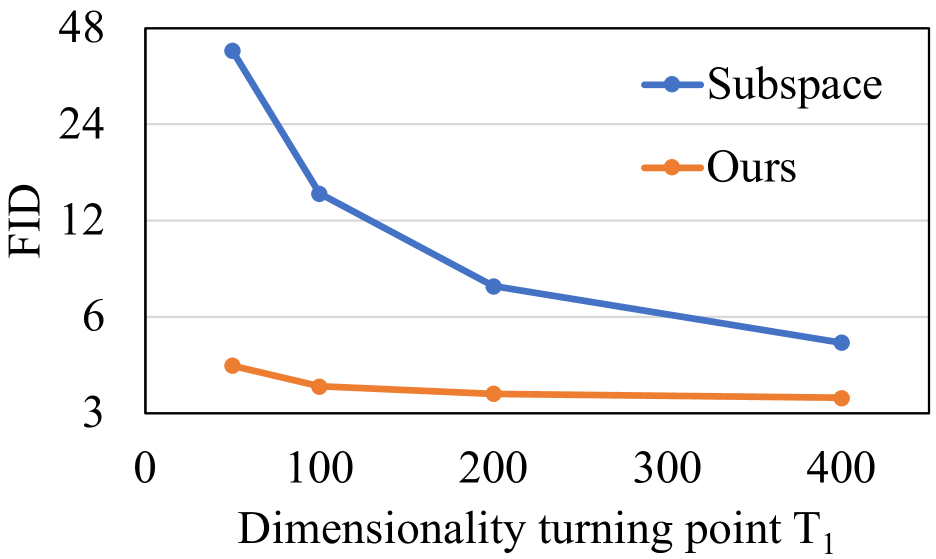
Fig. 4: Quantitative comparison between subspace diffusion [9] and our DVDP on CelebA 64$\times$64 regarding different dimensionality turning point $T_{1}$.

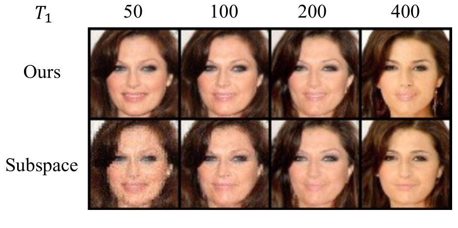
Fig. 5: Qualitative comparison between subspace diffusion [9] and our DVDP on CelebA 64$\times$64. $T_{1}$ denotes the dimensionality turning point.

5.4 Ablation Study

We implement ablation study in this section to show that DVDP is able to keep effective when the number of downsampling, i.e., $K$, grows. Specifically, we verify that on four different settings of dimensionality turning points ${\mathbb{T}}$ for $K=0,1,2,3$. When $K=1$, ${\mathbb{T}}$ is set to $\{250\}$. Similarly, when $K=2$ and $K=3$, ${\mathbb{T}}$ is set to $\{250,500\}$ and $\{250,500,750\}$, respectively. Furthermore, we use the same noise schedule for these four different settings. Tab. 3 shows that when the number of downsampling grows, the sampling quality preserves a reasonable level, indicating that DVDP can vary dimensionality for multiple times.

6 Conclusion

This paper generalizes the traditional diffusion process to a dimensionality-varying diffusion process (DVDP). The proposed DVDP has both theoretical and experimental contributions. Theoretically, we carefully decompose the signal in the diffusion process into multiple orthogonal dynamic attenuation components. With a rigorously deduced approximation strategy, this then leads to a novel reverse process that generates images from much lower dimensional noises compared with the image resolutions. This design allows much faster training and sampling speed of the diffusion models with on-par or even better synthesis performance, and superior performance in synthesizing large-size images of $1024\times 1024$ resolution compared with classic methods. The results in this work can promote the understanding and applications of diffusion models in broader scenarios.

Appendix

Appendix A Proofs and Derivations

A.1 Details on the Forward Transition Kernel

Here we prove that the marginal distributions of each forward ADP given by Eqs. 5 and 6 can be derived from the forward transition kernel defined by Eq. 7. The proof uses the following basic property of Gaussians

$${\mathbf{z}}_{1}\sim{\mathcal{N}}({\bm{\mu}};{\bm{\Sigma}}_{1}),~{}{\mathbf{z}}_{2}|{\mathbf{z}}_{1}\sim{\mathcal{N}}({\bm{A}}{\mathbf{z}}_{1};{\bm{\Sigma}}_{2})\Rightarrow{\mathbf{z}}_{2}\sim{\mathcal{N}}({\bm{A}}{\bm{\mu}};{\bm{A}}{\bm{\Sigma}}_{1}{\bm{A}}^{T}+{\bm{\Sigma}}_{2}).$$ (A1)

As a prerequisite, we first re-write the Gaussian transition kernel given by Eq. 7 as

$${\mathbf{x}}_{t}^{k}|{\mathbf{x}}_{t-1}^{k}\sim{\mathcal{N}}({\bm{U}}_{k}{\bm{\Lambda}}_{k,t}{\bm{U}}_{k}^{T}{\mathbf{x}}_{t-1}^{k};{\bm{U}}_{k}{\bm{L}}_{k,t}^{2}{\bm{U}}_{k}^{T}),~{}1\leq t\leq T,~{}0\leq k\leq K,$$ (A2)

where

$${\bm{\Lambda}}_{k,t} =\bar{{\bm{\Lambda}}}_{k,t-1}^{-1}\bar{{\bm{\Lambda}}}_{k,t},$$ (A3)

$${\bm{L}}_{k,t} =(\bar{{\bm{L}}}_{k,t}^{2}-{\bm{\Lambda}}_{k,t}^{2}\bar{{\bm{L}}}_{k,t-1}^{2})^{1/2}.$$

The marginal distributions given by Eqs. 5 and 6 can also be re-written as

$${\mathbf{x}}_{t}^{k}|{\mathbf{x}}_{0}^{k}\sim{\mathcal{N}}({\bm{U}}_{k}\bar{{\bm{\Lambda}}}_{k,t}{\bm{U}}_{k}^{T}{\mathbf{x}}_{0}^{k};{\bm{U}}_{k}\bar{{\bm{L}}}_{k,t}^{2}{\bm{U}}_{k}^{T}),~{}1\leq t\leq T,~{}0\leq k\leq K.$$ (A4)

With Eqs. A1 and A2, we can prove Eq. A4 by induction:

1. For $t=1$, ${\mathbf{x}}_{1}^{k}|{\mathbf{x}}_{0}^{k}\sim{\mathcal{N}}({\bm{U}}_{k}{\bm{\Lambda}}_{k,1}{\bm{U}}_{k}^{T}{\mathbf{x}}_{0}^{k};{\bm{U}}_{k}{\bm{L}}_{k,1}^{2}{\bm{U}}_{k}^{T})$ is directly defined by Eq. A2. It satisfies Eq. A4 since ${\bm{\Lambda}}_{k,1}=\bar{{\bm{\Lambda}}}_{k,1}$ and ${\bm{L}}_{k,1}=\bar{{\bm{L}}}_{k,1}$.

2. Suppose ${\mathbf{x}}_{t}^{k}|{\mathbf{x}}_{0}^{k}$ satisfies Eq. A4. With the definition of ${\mathbf{x}}_{t+1}^{k}|{\mathbf{x}}_{t}^{k}$ given by Eq. A2 and the property Eq. A1, ${\mathbf{x}}_{t+1}^{k}|{\mathbf{x}}_{0}^{k}$ can be derived as

   $${\mathbf{x}}_{t+1}^{k}|{\mathbf{x}}_{0}^{k}\sim {\mathcal{N}}({\bm{U}}_{k}{\bm{\Lambda}}_{k,t+1}\bar{{\bm{\Lambda}}}_{k,t}{\bm{U}}_{k}^{T}{\mathbf{x}}_{0}^{k};{\bm{U}}_{k}({\bm{\Lambda}}_{k,t+1}^{2}\bar{{\bm{L}}}_{k,t}^{2}+{\bm{L}}_{k,t+1}^{2}){\bm{U}}_{k}^{T})$$ (A5)

   $$= {\mathcal{N}}({\bm{U}}_{k}\bar{{\bm{\Lambda}}}_{k,t+1}{\bm{U}}_{k}^{T}{\mathbf{x}}_{0}^{k};{\bm{U}}_{k}\bar{{\bm{L}}}_{k,t+1}^{2}{\bm{U}}_{k}^{T}),$$

   where $\bar{{\bm{\Lambda}}}_{k,t+1}={\bm{\Lambda}}_{k,t+1}\bar{{\bm{\Lambda}}}_{k,t}$ and $\bar{{\bm{L}}}_{k,t+1}^{2}={\bm{\Lambda}}_{k,t+1}^{2}\bar{{\bm{L}}}_{k,t}^{2}+{\bm{L}}_{k,t+1}^{2}$ can be obtained from Eq. A3. Thus, ${\mathbf{x}}_{t+1}^{k}|{\mathbf{x}}_{0}^{k}$ also satisfies Eq. A4.

Thus, the proof is completed.

A.2 Derivation of $q({\mathbf{x}}_{t-1}^{k}|{\mathbf{x}}_{t}^{k},{\mathbf{x}}_{0}^{k})$

Here we derive $q({\mathbf{x}}_{t-1}^{k}|{\mathbf{x}}_{t}^{k},{\mathbf{x}}_{0}^{k})$ from the marginal distribution given by Eqs. 5 and 6 and the forward transition kernel given by Eq. 7. By the Bayes’ theorem, $q({\mathbf{x}}_{t-1}^{k}|{\mathbf{x}}_{t}^{k},{\mathbf{x}}_{0}^{k})\propto q({\mathbf{x}}_{t-1}^{k}|{\mathbf{x}}_{0}^{k})q({\mathbf{x}}_{t}^{k}|{\mathbf{x}}_{t-1}^{k},{\mathbf{x}}_{0}^{k})=q({\mathbf{x}}_{t-1}^{k}|{\mathbf{x}}_{0}^{k})q({\mathbf{x}}_{t}^{k}|{\mathbf{x}}_{t-1}^{k})$, where the equality holds because of the Markovian property of ${\mathbf{x}}_{0}^{k}\rightarrow{\mathbf{x}}_{1}^{k}\cdots\rightarrow{\mathbf{x}}_{T}^{k}$. With $q({\mathbf{x}}_{t-1}^{k}|{\mathbf{x}}_{0}^{k})$ and $q({\mathbf{x}}_{t}^{k}|{\mathbf{x}}_{t-1}^{k})$ given by Eqs. (5) to (7), we have

$$\log q({\mathbf{x}}_{t-1}^{k}|{\mathbf{x}}_{t}^{k},{\mathbf{x}}_{0}^{k})= \log q({\mathbf{x}}_{t-1}^{k}|{\mathbf{x}}_{0}^{k})+\log q({\mathbf{x}}_{t}^{k}|{\mathbf{x}}_{t-1}^{k})+C_{1}$$ (A6)

$$= -\frac{1}{2}({\mathbf{x}}_{t-1}^{k}-{\bm{U}}_{k}\bar{{\bm{\Lambda}}}_{k,t-1}{\bm{U}}_{k}^{T}{\mathbf{x}}_{0}^{k})^{T}{\bm{U}}_{k}\bar{{\bm{L}}}_{k,t-1}^{-2}{\bm{U}}_{k}^{T}({\mathbf{x}}_{t-1}^{k}-{\bm{U}}_{k}\bar{{\bm{\Lambda}}}_{k,t-1}{\bm{U}}_{k}^{T}{\mathbf{x}}_{0}^{k})$$

$$-\frac{1}{2}({\mathbf{x}}_{t}^{k}-{\bm{U}}_{k}{\bm{\Lambda}}_{k,t}{\bm{U}}_{k}^{T}{\mathbf{x}}_{t-1}^{k})^{T}{\bm{U}}_{k}{\bm{L}}_{k,t}^{-2}{\bm{U}}_{k}^{T}({\mathbf{x}}_{t}^{k}-{\bm{U}}_{k}{\bm{\Lambda}}_{k,t}{\bm{U}}_{k}^{T}{\mathbf{x}}_{t-1}^{k})+C_{2}$$

$$= -\frac{1}{2}\big{[}{{\mathbf{x}}_{t-1}^{k}}^{T}{\bm{U}}_{k}(\bar{{\bm{L}}}_{k,t-1}^{-2}+{\bm{\Lambda}}_{k,t}^{2}{\bm{L}}_{k,t}^{-2}){\bm{U}}_{k}^{T}{\mathbf{x}}_{t-1}^{k}$$

$$-2({\bm{U}}_{k}\bar{{\bm{\Lambda}}}_{k,t-1}\bar{{\bm{L}}}_{k,t-1}^{-2}{\bm{U}}_{k}^{T}{\mathbf{x}}_{0}^{k}+{\bm{U}}_{k}{\bm{\Lambda}}_{k,t}{\bm{L}}_{k,t}^{-2}{\bm{U}}_{k}^{T}{\mathbf{x}}_{t}^{k})^{T}{\mathbf{x}}_{t-1}^{k}\big{]}+C_{3}$$

$$= -\frac{1}{2}\big{[}{{\mathbf{x}}_{t-1}^{k}}^{T}{\bm{U}}_{k}{\bm{L}}_{k,t}^{-2}\bar{{\bm{L}}}_{k,t-1}^{-2}\bar{{\bm{L}}}_{k,t}^{2}{\bm{U}}_{k}^{T}{\mathbf{x}}_{t-1}^{k}$$

$$-2({\bm{U}}_{k}\bar{{\bm{\Lambda}}}_{k,t-1}\bar{{\bm{L}}}_{k,t-1}^{-2}{\bm{U}}_{k}^{T}{\mathbf{x}}_{0}^{k}+{\bm{U}}_{k}{\bm{\Lambda}}_{k,t}{\bm{L}}_{k,t}^{-2}{\bm{U}}_{k}^{T}{\mathbf{x}}_{t}^{k})^{T}{\mathbf{x}}_{t-1}^{k}\big{]}+C_{3}$$

$$= -\frac{1}{2}({\mathbf{x}}_{t-1}^{k}-\tilde{{\bm{\mu}}}_{k,t})^{T}\tilde{{\bm{\Sigma}}}_{k,t}^{-2}({\mathbf{x}}_{t-1}^{k}-\tilde{{\bm{\mu}}}_{k,t})+C_{4},$$

where $C_{1}$, $C_{2}$, $C_{3}$ and $C_{4}$ are constants that do not depend on ${\mathbf{x}}_{t-1}^{k}$, and

$$\tilde{{\bm{\mu}}}_{k,t}= \tilde{{\bm{\mu}}}_{k,t}({\mathbf{x}}_{t}^{k},{\mathbf{x}}_{0}^{k})={\bm{U}}_{k}\bar{{\bm{\Lambda}}}_{k,t-1}{\bm{L}}_{k,t}^{2}\bar{{\bm{L}}}_{k,t}^{-2}{\bm{U}}_{k}^{T}{\mathbf{x}}_{0}^{k}+{\bm{U}}_{k}{\bm{\Lambda}}_{k,t}\bar{{\bm{L}}}_{k,t-1}^{2}\bar{{\bm{L}}}_{k,t}^{-2}{\bm{U}}_{k}^{T}{\mathbf{x}}_{t}^{k},$$ (A7)

$$\tilde{{\bm{\Sigma}}}_{k,t}= {\bm{U}}_{k}{\bm{L}}_{k,t}^{2}\bar{{\bm{L}}}_{k,t-1}^{2}\bar{{\bm{L}}}_{k,t}^{-2}{\bm{U}}_{k}^{T}.$$

Thus, $q({\mathbf{x}}_{t-1}^{k}|{\mathbf{x}}_{t}^{k},{\mathbf{x}}_{0}^{k})={\mathcal{N}}({\mathbf{x}}_{t-1}^{k};\tilde{{\bm{\mu}}}_{k,t},\tilde{{\bm{\Sigma}}}_{k,t})$.

A.3 Derivation of the Loss Function

Here we derive Eq. 12 from the variational bound on negative log-likelihood

$$\mathbb{E}_{q}[-\log p_{\theta}({\mathbf{x}}_{0}^{0})]\leq \mathbb{E}_{q}\left[-\log\frac{p_{\theta}({\mathbf{x}}_{0:T_{1}}^{0},{\mathbf{x}}_{T_{1}:T_{2}}^{1},\cdots,{\mathbf{x}}_{T_{K}:T}^{K})}{q({\mathbf{x}}_{1:T_{1}}^{0},{\mathbf{x}}_{T_{1}:T_{2}}^{1},\cdots,{\mathbf{x}}_{T_{K}:T}^{K}|{\mathbf{x}}_{0}^{0})}\right]$$ (A8)

$$= \mathbb{E}_{q}\left[-\log\frac{p_{\theta}({\mathbf{x}}_{0}^{0}|{\mathbf{x}}_{1}^{0})p_{\theta}({\mathbf{x}}_{1:T_{1}}^{0},{\mathbf{x}}_{T_{1}:T_{2}}^{1},\cdots,{\mathbf{x}}_{T_{K}:T-1}^{K}|{\mathbf{x}}_{T}^{K})p_{\theta}({\mathbf{x}}_{T}^{K})}{q({\mathbf{x}}_{1:T_{1}}^{0},{\mathbf{x}}_{T_{1}:T_{2}}^{1},\cdots,{\mathbf{x}}_{T_{K}:T-1}^{K}|{\mathbf{x}}_{T}^{K},{\mathbf{x}}_{0}^{0})q({\mathbf{x}}_{T}^{K}|{\mathbf{x}}_{0}^{0})}\right]$$

$$= \mathbb{E}_{q}\Bigg{[}-\log p_{\theta}({\mathbf{x}}_{0}^{0}|{\mathbf{x}}_{1}^{0})-\sum_{k=0}^{K}\sum_{\begin{subarray}{c}t=T_{k}+1\\ t>1\end{subarray}}^{T_{k+1}}\log\frac{p_{\theta}({\mathbf{x}}_{t-1}^{k}|{\mathbf{x}}_{t}^{k})}{q({\mathbf{x}}_{t-1}^{k}|{\mathbf{x}}_{t}^{k},{\mathbf{x}}_{0}^{0})}$$

$$\qquad-\sum_{k=1}^{K}\log\frac{p_{\theta}({\mathbf{x}}_{T_{k}}^{k-1}|{\mathbf{x}}_{T_{k}}^{k})}{q({\mathbf{x}}_{T_{k}}^{k-1}|{\mathbf{x}}_{T_{k}}^{k},{\mathbf{x}}_{0}^{0})}-\log\frac{p_{\theta}({\mathbf{x}}_{T}^{K})}{q({\mathbf{x}}_{T}^{K}|{\mathbf{x}}_{0}^{0})}\Bigg{]}$$

$$= \mathbb{E}_{q}\Bigg{[}\underbrace{-\log p_{\theta}({\mathbf{x}}_{0}^{0}|{\mathbf{x}}_{1}^{0})}_{L_{0}}+\sum_{k=0}^{K}\sum_{\begin{subarray}{c}t=T_{k}+1\\ t>1\end{subarray}}^{T_{k+1}}\underbrace{{\rm D_{KL}}(q({\mathbf{x}}_{t-1}^{k}|{\mathbf{x}}_{t}^{k},{\mathbf{x}}_{0}^{k})\|p_{\theta}({\mathbf{x}}_{t-1}^{k}|{\mathbf{x}}_{t}^{k}))}_{L_{t-1}}$$

$$\qquad+\sum_{k=1}^{K}\underbrace{{\rm D_{KL}}(q({\mathbf{x}}_{T_{k}}^{k-1}|{\mathbf{x}}_{T_{k}}^{k},{\mathbf{x}}_{0}^{k-1})\|p_{\theta}({\mathbf{x}}_{T_{k}}^{k-1}|{\mathbf{x}}_{T_{k}}^{k}))}_{L_{k}^{\text{down}}}+\underbrace{{\rm D_{KL}}(q({\mathbf{x}}_{T}^{K}|{\mathbf{x}}_{0}^{0})\|p_{\theta}({\mathbf{x}}_{T}^{K}))}_{L_{T}}\Bigg{]},$$

where $L_{0},L_{T}$ and $L_{t-1},~{}t=2,3,\cdots,T$ are similar with the definitions in DDPM [6], and $L_{k}^{\text{down}}$ is a new term and can be viewed as the loss at the dimensionality turning point $T_{k}$. As defined in Eq. 11, $p_{\theta}({\mathbf{x}}_{T_{k}}^{k-1}|{\mathbf{x}}_{T_{k}}^{k}))$ has no learnable parameters, so we do not optimize $L_{k}^{\text{down}}$.

As for $L_{t-1}$, it is the KL divergence of two Gaussians and can be calculated as

$$L_{t-1}=\mathbb{E}_{q}\bigg{[}\frac{1}{2}\|{\bm{\Sigma}}_{t}^{-1/2}{\bm{U}}_{k}^{T}(\tilde{{\bm{\mu}}}_{k,t}({\mathbf{x}}_{t}^{k},{\mathbf{x}}_{0}^{k})-{\bm{\mu}}_{\theta}({\mathbf{x}}_{t}^{k},t))\|^{2}\bigg{]}+C,$$ (A9)

where $C$ is a constant that does not depend on $\theta$, $k$ satisfies $T_{k}<t\leq T_{k+1}$, $\tilde{{\bm{\mu}}}_{k,t}({\mathbf{x}}_{t}^{k},{\mathbf{x}}_{0}^{k})$ is the mean of $q({\mathbf{x}}_{t-1}^{k}|{\mathbf{x}}_{t}^{k},{\mathbf{x}}_{0}^{k})$ given by Eq. A7, and ${\bm{\mu}}_{\theta}$ is the mean of $p_{\theta}({\mathbf{x}}_{t-1}^{k}|{\mathbf{x}}_{t}^{k})$ given by Eq. 10.

With Eqs. 5 and 6, $L_{t-1}$ can be represented by reparameterization trick as

$$L_{t-1}= \mathbb{E}_{{\mathbf{x}}_{0}^{k},{\mathbf{\epsilon}}^{k}}\bigg{[}\frac{1}{2}\big{\|}{\bm{\Sigma}}_{t}^{-1/2}{\bm{U}}_{k}^{T}(\tilde{{\bm{\mu}}}_{k,t}({\mathbf{x}}_{t}^{k}({\mathbf{x}}_{0}^{k},{\mathbf{\epsilon}}^{k}),{\bm{U}}_{k}\bar{{\bm{\Lambda}}}_{k,t}^{-1}{\bm{U}}_{k}^{T}{\mathbf{x}}_{t}^{k}({\mathbf{x}}_{0}^{k},{\mathbf{\epsilon}}^{k})-{\bm{U}}_{k}\bar{{\bm{\Lambda}}}_{k,t}^{-1}\bar{{\bm{L}}}_{k,t}{\bm{U}}_{k}^{T}{\bm{\epsilon}}^{k})$$ (A10)

$$-{\bm{\mu}}_{\theta}({\mathbf{x}}_{t}^{k}({\mathbf{x}}_{0}^{k},{\mathbf{\epsilon}}^{k}),t))\big{\|}^{2}\bigg{]}+C$$

$$= \mathbb{E}_{{\mathbf{x}}_{0}^{k},{\mathbf{\epsilon}}^{k}}\bigg{[}\big{\|}{\bm{W}}_{t}({\mathbf{\epsilon}}^{k}-{\mathbf{\epsilon}}_{\theta}({\mathbf{x}}_{t}^{k}({\mathbf{x}}_{0}^{k},{\mathbf{\epsilon}}^{k}),t))\big{\|}^{2}\bigg{]}+C,$$

where the final equality is obtained by plugging Eq. 10 and Eq. A7 into it, and ${\bm{W}}_{t}=\frac{1}{\sqrt{2}}{\bm{\Sigma}}_{t}^{-1/2}{\bm{\Lambda}}_{k,t}^{-1}{\bm{L}}_{k,t}^{2}\bar{{\bm{L}}}_{k,t}^{-1}{\bm{U}}_{k}^{T}$.

Finally, by setting ${\bm{W}}_{t}={\bm{I}}$ as in DDPM [6], we can obtain Eq. 12.

A.4 Proof of Proposition 1

According to the inequality between JSD and total variation, we have

$${\rm JSD}(p_{1}||p_{2})\leq\frac{1}{2}\int|p_{1}(x)-p_{2}(x)|d{\bm{x}}.$$ (A11)

The RHS (right-hand side) of Eq. A11 satisfies

$$\frac{1}{2}\int|p_{1}({\bm{x}})-p_{2}({\bm{x}})|d{\bm{x}}= \frac{1}{2}\int\left|\mathbb{E}_{{\mathbf{x}}_{0}\sim p}[p_{1}({\bm{x}}|{\mathbf{x}}_{0})-p_{2}({\bm{x}}|{\mathbf{x}}_{0})]\right|d{\bm{x}}$$ (A12)

$$\leq \frac{1}{2}\int\mathbb{E}_{{\mathbf{x}}_{0}\sim p}\left[\left|p_{1}({\bm{x}}|{\mathbf{x}}_{0})-p_{2}({\bm{x}}|{\mathbf{x}}_{0})\right|\right]d{\bm{x}}$$

$$= \frac{1}{2}C_{1}\int\mathbb{E}_{{\mathbf{x}}_{0}\sim p}\bigg{[}\Big{|}\exp\big{(}-\frac{1}{2}({\bm{x}}-{\bm{A}}_{1}{\mathbf{x}}_{0})^{T}\Sigma^{-1}({\bm{x}}-{\bm{A}}_{1}{\mathbf{x}}_{0})\big{)}$$

$$-\exp\big{(}-\frac{1}{2}({\bm{x}}-{\bm{A}}_{2}{\mathbf{x}}_{0})^{T}\Sigma^{-1}({\bm{x}}-{\bm{A}}_{2}{\mathbf{x}}_{0})\big{)}\Big{|}\bigg{]}d{\bm{x}},$$

where $C_{1}=(2\pi)^{-1/2}{\rm det}({\bm{\Sigma}})^{-1/2}$.

According to the mean value theorem, for each ${\mathbf{x}}_{0}$ and ${\bm{x}}$, there exists $\theta=\theta({\mathbf{x}}_{0},{\bm{x}})\in[0,1]$ such that ${\bm{\xi}}=\theta({\bm{x}}-{\bm{A}}_{1}{\mathbf{x}}_{0})+(1-\theta)({\bm{x}}-{\bm{A}}_{2}{\mathbf{x}}_{0})={\bm{x}}-[\theta{\bm{A}}_{1}+(1-\theta){\bm{A}}_{2}]{\mathbf{x}}_{0}$ satisfies

$$\exp\big{(}-\frac{1}{2}({\bm{x}}-{\bm{A}}_{1}{\mathbf{x}}_{0})^{T}\Sigma^{-1}({\bm{x}}-{\bm{A}}_{1}{\mathbf{x}}_{0})\big{)}-\exp\big{(}-\frac{1}{2}({\bm{x}}-{\bm{A}}_{2}{\mathbf{x}}_{0})^{T}\Sigma^{-1}({\bm{x}}-{\bm{A}}_{2}{\mathbf{x}}_{0})\big{)}$$ (A13)

$$= {\bm{\xi}}^{T}{\bm{\Sigma}}^{-1}({\bm{A}}_{1}-{\bm{A}}_{2}){\mathbf{x}}_{0}\exp\big{(}-\frac{1}{2}{\bm{\xi}}^{T}{\bm{\Sigma}}^{-1}{\bm{\xi}}\big{)}$$

$$= F\cdot\exp\big{(}-\frac{1}{4}{\bm{\xi}}^{T}{\bm{\Sigma}}^{-1}{\bm{\xi}}\big{)},$$

where $F={\bm{\xi}}^{T}{\bm{\Sigma}}^{-1}({\bm{A}}_{1}-{\bm{A}}_{2}){\mathbf{x}}_{0}\exp\big{(}-\frac{1}{4}{\bm{\xi}}^{T}{\bm{\Sigma}}^{-1}{\bm{\xi}}\big{)}$, and $|F|$ satisfies the following inequality

$$|F|= \Big{|}\frac{({\bm{\Sigma}}^{1/2}{\bm{\xi}})^{T}}{\|{\bm{\Sigma}}^{-1/2}{\bm{\xi}}\|_{2}}{\bm{\Sigma}}^{-1/2}({\bm{A}}_{1}-{\bm{A}}_{2}){\mathbf{x}}_{0}\Big{|}\cdot\|{\bm{\Sigma}}^{-1/2}{\bm{\xi}}\|_{2}\exp\big{(}-\frac{1}{4}\|{\bm{\Sigma}}^{-1/2}{\bm{\xi}}\|_{2}^{2}\big{)}$$ (A14)

$$\leq C_{2}\|{\bm{\Sigma}}^{-1/2}({\bm{A}}_{1}-{\bm{A}}_{2}){\mathbf{x}}_{0}\|_{2}$$

$$\leq C_{2}B\|{\bm{\Sigma}}^{-1/2}({\bm{A}}_{1}-{\bm{A}}_{2})\|_{2},$$

where $C_{2}=\max_{a\geq 0}ae^{-\frac{1}{4}a^{2}}=\sqrt{2}e^{-\frac{1}{2}}$, and $B$ is the upper bound of $\|{\mathbf{x}}_{0}\|_{2}$ as assumption.

Combining Eqs. A12, LABEL:eq:prop1-p1-p2-diff and A14, we have

$$\frac{1}{2}\int|p_{1}({\bm{x}})-p_{2}({\bm{x}})|d{\bm{x}}\leq \frac{1}{2}C_{1}C_{2}B\|{\bm{\Sigma}}^{-1/2}({\bm{A}}_{1}-{\bm{A}}_{2})\|_{2}\int\mathbb{E}_{{\mathbf{x}}_{0}\sim p}\Big{[}\exp\big{(}-\frac{1}{4}{\bm{\xi}}^{T}{\bm{\Sigma}}^{-1}{\bm{\xi}}\big{)}\Big{]}d{\bm{x}},$$ (A15)

where ${\bm{\xi}}={\bm{x}}-[\theta{\bm{A}}_{1}+(1-\theta){\bm{A}}_{2}]{\mathbf{x}}_{0}$. Now we only need to prove that the RHS of Eq. A15 $\leq$ the LHS (left-hand side) of Eq. 13.

Let ${\mathbf{z}}={\bm{\Sigma}}^{-1/2}[\theta{\bm{A}}_{1}+(1-\theta){\bm{A}}_{2}]{\mathbf{x}}_{0}$, then ${\bm{\xi}}^{T}{\bm{\Sigma}}^{-1}{\bm{\xi}}=\|{\bm{\Sigma}}^{-1/2}{\bm{x}}-{\mathbf{z}}\|_{2}^{2}$, and ${\mathbf{z}}$ satisfies

$$\|{\mathbf{z}}\|_{2}= \|{\bm{\Sigma}}^{-1/2}[\theta{\bm{A}}_{1}+(1-\theta){\bm{A}}_{2}]{\mathbf{x}}_{0}\|_{2}$$ (A16)

$$\leq B\|{\bm{\Sigma}}^{-1/2}[\theta{\bm{A}}_{1}+(1-\theta){\bm{A}}_{2}]\|_{2}$$

$$\leq B\|{\bm{\Sigma}}^{-1/2}{\bm{A}}_{1}\|_{2},$$

where the last inequality is derived from the assumption that ${\bm{A}}_{1}\succeq{\bm{A}}_{2}\succeq{\bm{0}}$.

Let ${\mathbb{D}}=\{{\bm{x}}:\|{\bm{\Sigma}}^{-1/2}{\bm{x}}\|_{2}\leq r\}$, where $r=2B\|{\bm{\Sigma}}^{-1/2}{\bm{A}}_{1}\|_{2}$, thus $\|{\mathbf{z}}\|_{2}\leq\frac{1}{2}r$ according to Eq. A16. Then the integration in Eq. A15 can be split into two regions as

$$\int\mathbb{E}_{{\mathbf{x}}_{0}\sim p}\Big{[}\exp\big{(}-\frac{1}{4}{\bm{\xi}}^{T}{\bm{\Sigma}}^{-1}{\bm{\xi}}\big{)}\Big{]}d{\bm{x}}= \int_{\mathbb{D}}\mathbb{E}_{{\mathbf{x}}_{0}\sim p}\Big{[}\exp\big{(}-\frac{1}{4}\|{\bm{\Sigma}}^{-1/2}{\bm{x}}-{\mathbf{z}}\|_{2}^{2}\big{)}\Big{]}d{\bm{x}}$$ (A17)

$$+\int_{{\mathbb{D}}^{\rm C}}\mathbb{E}_{{\mathbf{x}}_{0}\sim p}\Big{[}\exp\big{(}-\frac{1}{4}\|{\bm{\Sigma}}^{-1/2}{\bm{x}}-{\mathbf{z}}\|_{2}^{2}\big{)}\Big{]}d{\bm{x}}$$

$$\leq \int_{\mathbb{D}}1d{\bm{x}}+\int\exp\big{(}-\frac{1}{16}\|{\bm{\Sigma}}^{-1/2}{\bm{x}}\|_{2}^{2}\big{)}d{\bm{x}}$$

$$\leq V_{d}(r){\rm det}(\Sigma)^{1/2}+2\sqrt{2}(2\pi)^{d/2}{\rm det}(\Sigma)^{1/2},$$

where $V_{d}(\cdot)$ is the volume of $d$-dimensional sphere with respect to the radius.

Combining Eqs. A11, A15 and A17, we can get Proposition 1.

A.5 Proof of Theorem 1

We first prove that $q({\mathbf{x}}_{T_{k}}^{k-1})$ and $p({\mathbf{x}}_{T_{k}}^{k-1})$ defined in Theorem 1 satisfy the conditions claimed in Proposition 1.

$q({\mathbf{x}}_{T_{k}}^{k})$ is the marginal distribution of $q({\mathbf{x}}_{0}^{k})q({\mathbf{x}}_{T_{k}}^{k}|{\mathbf{x}}_{0}^{k})$ where $q({\mathbf{x}}_{T_{k}}^{k}|{\mathbf{x}}_{0}^{k})$ is defined by Eqs. 5 and 6. $q({\mathbf{x}}_{T_{k}}^{k}|{\mathbf{x}}_{0}^{k})$ can also be expressed as

$$q({\mathbf{x}}_{T_{k}}^{k}|{\mathbf{x}}_{0}^{k})={\mathcal{N}}({\mathbf{x}}_{T_{k}}^{k};{\bm{U}}_{k}\bar{{\bm{\Lambda}}}_{k,T_{k}}{\bm{U}}_{k}^{T}{\mathbf{x}}_{0}^{k},{\bm{U}}_{k}\bar{{\bm{L}}}_{k,T_{k}}^{2}{\bm{U}}_{k}^{T}).$$ (A18)

Similarly, $q({\mathbf{x}}_{T_{k}}^{k-1})$ is the marginal distribution of $q({\mathbf{x}}_{0}^{k-1})q({\mathbf{x}}_{T_{k}}^{k-1}|{\mathbf{x}}_{0}^{k-1})$ where $q({\mathbf{x}}_{T_{k}}^{k-1}|{\mathbf{x}}_{0}^{k-1})$ can be expressed as

$$q({\mathbf{x}}_{T_{k}}^{k-1}|{\mathbf{x}}_{0}^{k-1})={\mathcal{N}}({\mathbf{x}}_{T_{k}}^{k-1};{\bm{U}}_{k-1}\bar{{\bm{\Lambda}}}_{{k-1},T_{k}}{\bm{U}}_{k-1}^{T}{\mathbf{x}}_{0}^{k-1},{\bm{U}}_{k-1}\bar{{\bm{L}}}_{{k-1},T_{k}}^{2}{\bm{U}}_{k-1}^{T}).$$ (A19)

By definition, $p({\mathbf{x}}_{T_{k}}^{k-1})$ is the marginal distribution of $q({\mathbf{x}}_{T_{k}}^{k})p({\mathbf{x}}_{T_{k}}^{k-1}|{\mathbf{x}}_{T_{k}}^{k})$, where $p({\mathbf{x}}_{T_{k}}^{k-1}|{\mathbf{x}}_{T_{k}}^{k})$ is defined by Eq. 11 and can be expressed as

$$p({\mathbf{x}}_{T_{k}}^{k-1}|{\mathbf{x}}_{T_{k}}^{k})={\mathcal{N}}({\mathbf{x}}_{T_{k}}^{k-1};{\mathcal{D}}_{k}^{T}{\mathbf{x}}_{T_{k}}^{k},{\bm{U}}_{k-1}\Delta{\bm{L}}_{k-1}^{2}{\bm{U}}_{k-1}^{T}).$$ (A20)

To transform $p({\mathbf{x}}_{T_{k}}^{k-1})$ into the form in Proposition 1, we construct a Markov chain ${\mathbf{x}}_{0}^{k-1}\rightarrow{\mathbf{x}}_{T_{k}}^{k}\rightarrow{\mathbf{x}}_{T_{k}}^{k-1}$, where ${\mathbf{x}}_{0}^{k-1}\sim q({\mathbf{x}}_{0}^{k-1})$, ${\mathbf{x}}_{T_{k}}^{k}|{\mathbf{x}}_{0}^{k-1}\sim q({\mathbf{x}}_{T_{k}}^{k}|{\mathbf{x}}_{0}^{k-1})=q({\mathbf{x}}_{T_{k}}^{k}|{\mathcal{D}}_{k}{\mathbf{x}}_{0}^{k-1})$ and ${\mathbf{x}}_{T_{k}}^{k-1}|{\mathbf{x}}_{T_{k}}^{k}\sim p({\mathbf{x}}_{T_{k}}^{k-1}|{\mathbf{x}}_{T_{k}}^{k})$. Thus $p({\mathbf{x}}_{T_{k}}^{k-1})$ is also the marginal distribution of the joint distribution defined by the Markov chain. This joint distribution can be factorized as $q({\mathbf{x}}_{0}^{k-1})p_{q}({\mathbf{x}}_{T_{k}}^{k-1}|{\mathbf{x}}_{0}^{k-1})$, where $p_{q}({\mathbf{x}}_{T_{k}}^{k-1}|{\mathbf{x}}_{0}^{k-1})$ is the marginal distribution of $q({\mathbf{x}}_{T_{k}}^{k}|{\mathbf{x}}_{0}^{k-1})p({\mathbf{x}}_{T_{k}}^{k-1}|{\mathbf{x}}_{T_{k}}^{k})$, and can be derived from Eqs. A18 and A20 by using Eq. A1

$$p_{q}({\mathbf{x}}_{T_{k}}^{k-1}|{\mathbf{x}}_{0}^{k-1})= {\mathcal{N}}({\mathbf{x}}_{T_{k}}^{k-1};{\mathcal{D}}_{k}^{T}{\bm{U}}_{k}\bar{{\bm{\Lambda}}}_{k,T_{k}}{\bm{U}}_{k}^{T}{\mathcal{D}}_{k}{\mathbf{x}}_{0}^{k-1},{\bm{U}}_{k-1}\Delta{\bm{L}}_{k-1}^{2}{\bm{U}}_{k-1}^{T}+{\mathcal{D}}_{k}^{T}{\bm{U}}_{k}\bar{{\bm{L}}}_{k,T_{k}}^{2}{\bm{U}}_{k}^{T}{\mathcal{D}}_{k})$$ (A21)

$$= {\mathcal{N}}({\mathbf{x}}_{T_{k}}^{k-1};{\bm{U}}_{k-1}(\bar{{\bm{\Lambda}}}_{k-1,T_{k}}-\Delta{\bm{\Lambda}}_{k-1}){\bm{U}}_{k-1}^{T}{\mathbf{x}}_{0}^{k-1},{\bm{U}}_{k-1}{\bm{L}}_{k-1,T_{k}}^{2}{\bm{U}}_{k-1}^{T}),$$

where $\Delta{\bm{\Lambda}}_{k-1}={\rm diag}(\bar{\lambda}_{k-1,T_{k}}{\bm{I}}_{d_{k-1}},{\bm{O}}_{\bar{d}_{k}})$.

Thus, $q({\mathbf{x}}_{T_{k}}^{k-1}|{\mathbf{x}}_{0}^{k-1})$ given by Eq. A19 and $p_{q}({\mathbf{x}}_{T_{k}}^{k-1}|{\mathbf{x}}_{0}^{k-1})$ given by Eq. A21 satisfy conditions of $p_{1}$ and $p_{2}$ claimed in Proposition 1 respectively. And $\|{\mathbf{x}}_{0}^{k-1}\|$ satisfies

$$\|{\mathbf{x}}_{0}^{k-1}\|=\|\overline{{\mathcal{D}}}_{k-1}{\mathbf{x}}_{0}^{0}\|\leq\|{\mathbf{x}}_{0}^{0}\|\leq\sqrt{d}.$$ (A22)

Finally, substituting all corresponding variables into Eq. 13, we can obtain Eq. 14.

Appendix B Implementation Details

In this section, we will give more details on the implementation of our DVDP. Algs. 1 and 2 display the complete training and sampling procedures respectively.

Algorithm 1 Training

1:repeat

2:     Sample $k$ from $(\{0,\cdots,K\})$

3:     $t\sim{\rm Uniform}(\{T_{k}+1,\cdots,T_{k+1}\})$

4:     ${\mathbf{x}}_{0}^{0}\sim q({\mathbf{x}}_{0}^{0})$

5:     ${\mathbf{\epsilon}}^{k}\sim{\mathcal{N}}({\bm{0}};{\bm{I}}_{\bar{d}_{k}})$

6:     ${\mathbf{x}}_{0}^{k}\leftarrow\overline{{\mathcal{D}}}_{k}{\mathbf{x}}_{0}^{0}$

7:     ${\mathbf{x}}_{t}^{k}\leftarrow{\bm{U}}_{k}\bar{{\bm{\Lambda}}}_{k,t}{\bm{U}}_{k}^{T}{\mathbf{x}}_{0}^{k}+{\bm{U}}_{k}\bar{{\bm{L}}}_{k,t}{\bm{U}}_{k}^{T}{\mathbf{\epsilon}}^{k}$

8:     Take gradient descent step on

9:   $\nabla_{\theta}\|{\mathbf{\epsilon}}^{k}-{\bm{\epsilon}}_{\theta}({\mathbf{x}}_{t}^{k},t)\|^{2}$

10:until converged

Algorithm 2 Sampling

1:${\mathbf{x}}_{T}^{K}\sim{\mathcal{N}}({\bm{0}};{\bm{I}}_{\bar{d}_{K}})$

2:for $k=K,\cdots,0$ do

3:     for $t=T_{k+1},\cdots,T_{k}+1$ do

4:         ${\mathbf{\epsilon}}^{k}\sim{\mathcal{N}}({\bm{0}};{\bm{I}}_{\bar{d}_{k}})$

5:         ${\mathbf{x}}_{t-1}^{k}\leftarrow{\bm{U}}_{k}\bar{{\bm{\Lambda}}}_{k,t}^{-1}({\bm{U}}_{k}^{T}{\mathbf{x}}_{t}^{k}-\bar{{\bm{L}}}_{k,t}{\bm{U}}_{k}^{T}{\bm{\epsilon}}_{\theta}({\mathbf{x}}_{t}^{k},t))+{\bm{\Sigma}}_{t}{\mathbf{\epsilon}}^{k}$      

6:     if $k>0$ then

7:         ${\mathbf{\epsilon}}^{k-1}\sim{\mathcal{N}}({\bm{0}};{\bm{I}}_{\bar{d}_{k-1}})$

8:         ${\mathbf{x}}_{T_{k}}^{k-1}\leftarrow{\mathcal{D}}_{k}^{T}{\mathbf{x}}_{T_{k}}^{k}+{\bm{U}}_{k-1}\Delta{\bm{L}}_{k-1}{\bm{U}}_{k-1}^{T}{\mathbf{\epsilon}}^{k-1}$      

9:return ${\mathbf{x}}_{0}^{0}$

B.1 Choice of Downsampling Operator ${\mathcal{D}}_{k}$

Since an image pixel is usually similar with its neighbours, we can simply choose ${\mathcal{D}}_{k}$ to be a $2\times 2$ average-pooling operator for each $k=1,\cdots,K$ as in subspace diffusion [9] to maintain the main component of an image. Under this choice, the dimensionality will be reduced from $\bar{d}_{k-1}$ to $\bar{d}_{k}=\frac{1}{4}\bar{d}_{k-1}$ after each downsampling operation, as mentioned in Sec. 5.1.

The above choice needs a simple modification, multiplication by 2 after the average-pooling operation, to ensure that the matrix ${\mathcal{D}}_{k}$ satisfies

$${\mathcal{D}}_{k}[{\bm{N}}_{k-1},{\bm{B}}_{k-1}]=[\bm{0},{\bm{U}}_{k}],$$ (A23)

where ${\bm{N}}_{k-1}\in{\mathbb{R}}^{\bar{d}_{k-1}\times d_{k-1}}$ and ${\bm{B}}_{k-1}\in{\mathbb{R}}^{\bar{d}_{k-1}\times\bar{d}_{k}}$ satisfies ${\bm{U}}_{k-1}=[{\bm{N}}_{k-1},{\bm{B}}_{k-1}]$. Under this condition, the matrix ${\mathcal{D}}_{k}\in{\mathbb{R}}^{\bar{d}_{k}\times\bar{d}k-1}$ is row-orthogonal, and ${\mathcal{D}}_{k}^{T}$ (i.e., the transpose of ${\mathcal{D}}_{k}$) is just the corresponding upsampling operator.

B.2 Attenuation Coefficient $\bar{\lambda}_{k,t}$

As mentioned in Sec. 4.1, only $\bar{\lambda}_{k,t}$ is required to be approximate zero at dimensionality turning point $T_{k+1}$ for $k=0,\cdots,K-1$, thus we only need to decrease $\bar{\lambda}_{k,t}$ when $T_{k}<t\leq T_{k+1}$ and keep $\bar{\lambda}_{i,t},~{}i\neq k$ unchanged. In experiment, we decrease $\bar{\lambda}_{k,t}$ in an exponential form. Thus, for $\bar{\lambda}_{k,t},~{}k=0,1,\cdots,K-1$, they are set in the following manner:

$$\bar{\lambda}_{k,t}=\begin{cases}1,&t\leq T_{k}\\ \bar{\lambda}_{\min},&t>T_{k+1}\\ \bar{\lambda}_{\min}^{(t-T_{k})/(T_{k+1}-T_{k})},&T_{k}<t\leq T_{k+1},\end{cases}$$ (A24)

where $\bar{\lambda}_{\min}\in(0,1)$ is a shared hyperparameters for $\bar{\lambda}_{0,t},\bar{\lambda}_{1,t},\cdots,\bar{\lambda}_{K-1,t}$. For all experiments, we set $\bar{\lambda}_{\min}=0.01$. As for $k=K$, we set $\bar{\lambda}_{K,t}=1$ for all $t$. This schedule means that between two adjacent dimensionality turning points $T_{k}$ and $T_{k+1}$, we only attenuate one data component ${\mathbf{v}}_{k}^{k}$. Once we set $\bar{\lambda}_{k,t}$ for each $k$ and $t$, hyperparameters ${\lambda}_{k,t},~{}\bar{{\bm{\Lambda}}}_{k,t},~{}{\bm{\Lambda}}_{k,t}$ are determined.

B.3 Noise Schedule $\bar{\sigma}_{k,t}$

At each timestep $t$, we set $\sigma_{0,t}=\sigma_{1,t}=\cdots,=\sigma_{K,t}\triangleq\sigma_{t}$, which means that the added noise at each step is symmetric, similar with that in DDPM [6]. Rather than setting $\sigma_{t}$ directly, we first determine $\bar{\sigma}_{t}=\sum_{s=1}^{t}\sigma_{s}$, then obtain $\sigma_{t}$ by $\sigma_{t}=\bar{\sigma}_{t}/\bar{\sigma}_{t-1}$.

Since we choose subspaces in which the main components of images stay, the image signal will not lose much components when getting close to the subspace and downsampled to a smaller size. However, Gaussian noise does not have this property and can lose large parts of components in the downsampling operation. Thus, the signal-to-noise (SNR) ratio at the last timestep $T$ will be smaller than that in DDPM [6] if we just use the same noise schedule. Suppose at $T_{k},~{}k=1,2,\cdots,K$, ${{\mathbf{y}}}_{{k-1},{T_{k}}}\in{\mathbb{R}}^{\bar{d}_{k-1}}$ is downsampled to ${{\mathbf{y}}}_{{k},{T_{k}}}\in{\mathbb{R}}^{\bar{d}_{k}}$ with downsamling factor $f_{k}=\bar{d}_{k-1}/\bar{d}_{k}$, then the noise shedule is adapted as Algorithm 3, which can approximately keep the SNR at the last timestep meanwhile maintaining the continuity of $\bar{\sigma}$.

Algorithm 3 Adaptation on Noise Schedule

1:Initialize $\bar{\alpha}_{0:T}$ as in DDPM

2:$\bar{\sigma}\leftarrow\sqrt{\frac{1}{\bar{\alpha}}-1}$

3:for $k=1,\cdots,K$ do

4:     $\bar{\sigma}_{T_{k}:T}\leftarrow\bar{\sigma}_{T_{k}-1}+f_{k}\cdot(\bar{\sigma}_{T_{k}:T}-\bar{\sigma}_{T_{k}-1})$

B.4 Simplification of Matrix Multiplication ${\bm{U}}_{k}{\bm{G}}_{k}{\bm{U}}_{k}^{T}$

With the above choices of attenuation coefficients and noise schedule, all matrix multiplications with the form of ${\bm{U}}_{k}{\bm{G}}_{k}{\bm{U}}_{k}^{T}$ in the implementation of DVDP can be expressed by downsampling operator ${\mathcal{D}}_{k+1}$ and upsampling operator ${\mathcal{D}}_{k+1}^{T}$, since each diagonal matrix ${\bm{G}}_{k}$ only includes two different elements and can be expressed in the form of ${\bm{G}}={\rm diag}(a_{k}{\bm{I}}_{d_{k}},b_{k}{\bm{I}}_{\bar{d}_{k+1}})$. Thus, ${\bm{U}}_{k}{\bm{G}}_{k}{\bm{U}}_{k}^{T}$ can be expressed as

$${\bm{U}}_{k}{\bm{G}}_{k}{\bm{U}}_{k}^{T}= [{\bm{N}}_{k},{\bm{B}}_{k]}]\begin{bmatrix}a_{k}{\bm{I}}_{d_{k}}&{\bm{0}}\\ {\bm{0}}&b_{k}{\bm{I}}_{\bar{d}_{k+1}}\end{bmatrix}[{\bm{N}}_{k},{\bm{B}}_{k]}]^{T}$$ (A25)

$$= a_{k}{\bm{I}}_{\bar{d}_{k}}+[{\bm{N}}_{k},{\bm{B}}_{k]}]\begin{bmatrix}{\bm{0}}&{\bm{0}}\\ {\bm{0}}&(b_{k}-a_{k}){\bm{I}}_{\bar{d}_{k+1}}\end{bmatrix}[{\bm{N}}_{k},{\bm{B}}_{k]}]^{T}$$

$$= a_{k}{\bm{I}}_{\bar{d}_{k}}+(b_{k}-a_{k}){\bm{B}}_{k}{\bm{B}}_{k}^{T}$$

$$= a_{k}{\bm{I}}_{\bar{d}_{k}}+(b_{k}-a_{k}){\mathcal{D}}_{k+1}^{T}{\mathcal{D}}_{k+1},$$

where the last equality can be derived from Eq. A23.

Appendix C Experiments on DDIM Sampling

To demonstrate that our DVDP is compatible with DDIM [25], an accelerated sampling method, we apply DDIM to our models trained on LSUN Church $256\times 256$ and FFQH $256\times 256$. The results are shown in Tab. A1. In experiment, we find that it is beneficial for DVDP to add noises in some middle steps of sampling, unlike DDIM that sets all inserted noises to zeros. Specifically, we set $\eta_{t}=1$ for $t=T_{1}-\lfloor T_{1}/4\rfloor,\cdots,T_{1}+\lceil(T_{2}-T_{1})/2\rceil$ and $\eta_{t}=0$ otherwise, where $\eta_{t}\in[0,1]$ controls the strength of added noise as in DDIM [25] for timestep $t$. This adaption is marked by ^∗ in Tab. A1.

Tab. A1: Quantitative comparison measured in FID. DDIM^∗ denotes an adapted DDIM sampling method.

Dataset	Church $256\times 256$			FFHQ $256\times 256$
#Steps	50	100	200	50	100	200
DDIM Baseline	10.44	10.22	10.26	12.32	10.80	10.19
DDIM∗ Baseline	9.36	8.91	9.03	13.33	10.28	9.06
DDIM∗ DVDP	8.52	7.33	7.32	12.01	8.39	7.04

References

- [1] F. Bao, C. Li, J. Zhu, and B. Zhang. Analytic-dpm: an analytic estimate of the optimal reverse variance in diffusion probabilistic models. Int. Conf. Learn. Represent., 2022.
- [2] P. Dhariwal and A. Nichol. Diffusion models beat gans on image synthesis. Adv. Neural Inform. Process. Syst., pages 8780–8794, 2021.
- [3] P. Esser, R. Rombach, A. Blattmann, and B. Ommer. Imagebart: Bidirectional context with multinomial diffusion for autoregressive image synthesis. Adv. Neural Inform. Process. Syst., pages 3518–3532, 2021.
- [4] K. He, X. Chen, S. Xie, Y. Li, P. Dollár, and R. Girshick. Masked autoencoders are scalable vision learners. In IEEE Conf. Comput. Vis. Pattern Recog., pages 16000–16009, 2022.
- [5] M. Heusel, H. Ramsauer, T. Unterthiner, B. Nessler, and S. Hochreiter. Gans trained by a two time-scale update rule converge to a local nash equilibrium. Adv. Neural Inform. Process. Syst., 2017.
- [6] J. Ho, A. Jain, and P. Abbeel. Denoising diffusion probabilistic models. In Adv. Neural Inform. Process. Syst., pages 6840–6851, 2020.
- [7] J. Ho, C. Saharia, W. Chan, D. J. Fleet, M. Norouzi, and T. Salimans. Cascaded diffusion models for high fidelity image generation. JMLR, pages 47–1, 2022.
- [8] M. Hu, Y. Wang, T.-J. Cham, J. Yang, and P. N. Suganthan. Global context with discrete diffusion in vector quantised modelling for image generation. In IEEE Conf. Comput. Vis. Pattern Recog., pages 11502–11511, 2022.
- [9] B. Jing, G. Corso, R. Berlinghieri, and T. Jaakkola. Subspace diffusion generative models. arXiv preprint arXiv:2205.01490, 2022.
- [10] T. Karras, S. Laine, and T. Aila. A style-based generator architecture for generative adversarial networks. In IEEE Conf. Comput. Vis. Pattern Recog., pages 4401–4410, 2019.
- [11] A. Krizhevsky, G. Hinton, et al. Learning multiple layers of features from tiny images. 2009.
- [12] S. Lee, H. Chung, J. Kim, and J. C. Ye. Progressive deblurring of diffusion models for coarse-to-fine image synthesis. arXiv preprint arXiv:2207.11192, 2022.
- [13] L. Liu, Y. Ren, Z. Lin, and Z. Zhao. Pseudo numerical methods for diffusion models on manifolds. arXiv preprint arXiv:2202.09778, 2022.
- [14] Z. Liu, P. Luo, X. Wang, and X. Tang. Deep learning face attributes in the wild. In Int. Conf. Comput. Vis., pages 3730–3738, 2015.
- [15] C. Lu, Y. Zhou, F. Bao, J. Chen, C. Li, and J. Zhu. Dpm-solver: A fast ode solver for diffusion probabilistic model sampling in around 10 steps. arXiv preprint arXiv:2206.00927, 2022.
- [16] T. Luhman and E. Luhman. Improving diffusion model efficiency through patching. arXiv preprint arXiv:2207.04316, 2022.
- [17] A. Q. Nichol and P. Dhariwal. Improved denoising diffusion probabilistic models. In Int. Conf. Mach. Learn., pages 8162–8171, 2021.
- [18] K. Preechakul, N. Chatthee, S. Wizadwongsa, and S. Suwajanakorn. Diffusion autoencoders: Toward a meaningful and decodable representation. In IEEE Conf. Comput. Vis. Pattern Recog., pages 10619–10629, 2022.
- [19] A. Ramesh, P. Dhariwal, A. Nichol, C. Chu, and M. Chen. Hierarchical text-conditional image generation with clip latents. arXiv preprint arXiv:2204.06125, 2022.
- [20] R. Rombach, A. Blattmann, D. Lorenz, P. Esser, and B. Ommer. High-resolution image synthesis with latent diffusion models. In IEEE Conf. Comput. Vis. Pattern Recog., pages 10684–10695, 2022.
- [21] D. Ryu and J. C. Ye. Pyramidal denoising diffusion probabilistic models. arXiv preprint arXiv:2208.01864, 2022.
- [22] C. Saharia, W. Chan, S. Saxena, L. Li, J. Whang, E. Denton, S. K. S. Ghasemipour, B. K. Ayan, S. S. Mahdavi, R. G. Lopes, et al. Photorealistic text-to-image diffusion models with deep language understanding. arXiv preprint arXiv:2205.11487, 2022.
- [23] R. San-Roman, E. Nachmani, and L. Wolf. Noise estimation for generative diffusion models. arXiv preprint arXiv:2104.02600, 2021.
- [24] J. Sohl-Dickstein, E. Weiss, N. Maheswaranathan, and S. Ganguli. Deep unsupervised learning using nonequilibrium thermodynamics. In Int. Conf. Mach. Learn., pages 2256–2265, 2015.
- [25] J. Song, C. Meng, and S. Ermon. Denoising diffusion implicit models. arXiv preprint arXiv:2010.02502, 2020.
- [26] Y. Song, J. Sohl-Dickstein, D. P. Kingma, A. Kumar, S. Ermon, and B. Poole. Score-based generative modeling through stochastic differential equations. Int. Conf. Learn. Represent., 2021.
- [27] A. Vahdat, K. Kreis, and J. Kautz. Score-based generative modeling in latent space. Adv. Neural Inform. Process. Syst., pages 11287–11302, 2021.
- [28] D. Watson, W. Chan, J. Ho, and M. Norouzi. Learning fast samplers for diffusion models by differentiating through sample quality. In Int. Conf. Learn. Represent., 2021.
- [29] D. Watson, J. Ho, M. Norouzi, and W. Chan. Learning to efficiently sample from diffusion probabilistic models. arXiv preprint arXiv:2106.03802, 2021.
- [30] F. Yu, A. Seff, Y. Zhang, S. Song, T. Funkhouser, and J. Xiao. Lsun: Construction of a large-scale image dataset using deep learning with humans in the loop. arXiv preprint arXiv:1506.03365, 2015.
- [31] Q. Zhang and Y. Chen. Diffusion normalizing flow. Adv. Neural Inform. Process. Syst., pages 16280–16291, 2021.