Graph based semi-supervised learning using spatial Segregation theory

Abstract.

In this work we address graph based semi-supervised learning using the theory of the spatial segregation of competitive systems. First, we define a discrete counterpart over connected graphs by using direct analogue of the corresponding competitive system. This model turns out doesn’t have a unique solution as we expected. Nevertheless, we suggest gradient projected and regularization methods to reach some of the solutions. Then we focus on a slightly different model motivated from the recent numerical results on the spatial segregation of reaction-diffusion systems. In this case we show that the model has a unique solution and propose a novel classification algorithm based on it. Finally, we present numerical experiments showing the method is efficient and comparable to other semi-supervised learning algorithms at high and low label rates.

1. Introduction

In this paper we consider a semi-supervised learning approach which deals with the classification of a large number of unlabeled data when very few labels just are available. In some applications such as medical images, we have few training examples which are labeled. The aim is to find efficient algorithms with good performance with these few labeled examples. In this situation, geometric or topological properties of the unlabeled data has been used to propose and to improve several algorithms.

A common way to use the unlabeled data in semi-supervised learning is to build a graph over the data e.g., in image classification. To start, we requires to construct an adjacency matrix, or weight matrix $W$, for the data set, which encodes the similarities between pairs of date nodes. If our data set consists of $n$ points ${\mathcal{X}}=\{x_{1},x_{2},\cdots,x_{n}\}\subset\mathbb{R}^{d}$, then the weight matrix $W$ is an $n\times n$ symmetric matrix, where the element $w_{ij}$ represents the similarity between two data points $x_{i}$ and $x_{j}$. The similarity is always nonnegative and should be large when $x_{i}$ and $x_{j}$ are close together spatially, and small (or zero), when $x_{i}$ and $x_{j}$ are far apart. As a choice, the weight matrix can be the Gaussian weights

$$w_{ij}=\textrm{exp}(-\frac{|x_{i}-x_{j}|}{2\sigma^{2}}),$$

where $|\cdot|$ is the Euclidean norm and $\sigma$ is a free parameter that controls the scale at which points are connected by strong similarities $w_{ij}$ in the weight matrix. In fact, the weight matrix $W$ provides the data set with a graph structure, where each pair of points $(x_{i},x_{j})$ is connected by an edge with edge weight $w_{ij}.$ Other choices of weight matrix are possible, such as the $k$-nearest neighbor graph, see [26].

Recently, many works aim to transpose and adapt Partial Differential Equations (PDEs) on graphs. This reformulation of continuous problems onto a graph is such that the solution behaves analogously to the continuous formulation see [6, 15].

In graph-based semi-supervised learning, we are given a few labeled data on the graph and we aim to extend these labels from a given set to the rest of the nodes in graph in a decisive manner. To model propagating labels in semi-supervised learning, it is assumed that the learned labels vary smoothly and not change fast within high density regions of the graph (smoothness assumptions). Based on this assumption different approaches have been proposed. One of the pioneer methods is Laplace learning, [27]. Later it has been observed that the Laplace learning can give poor results in classification [23]. The results are often poor because the solutions have localized spikes near the labeled points, while being almost constant far from them. To overcome this problem several versions of Laplace learning algorithm have been proposed, for instance Laplacian regularization, [1], weighted Laplacian, [25, 13] and $p$-Laplace learning, [11, 24]. Also, the limiting case in $p$-Laplacian when $p$ tends to infinity is so called Lipschitz learning is studied in [22] and similar to continuum PDEs is related to finding the absolutely minimal lipschitz extension of the training data. Recently, in [10] another approach to increase accuracy of Laplace learning is given and called Poisson learning.

To explain these methods, let as before ${\mathcal{X}}={\{x_{1},\cdots,x_{n}}\}$ denotes the data points or equivalently vertices in a graph. We assume there is a subset of the nodes $\Gamma={\{x_{1},\cdots,x_{m}}\}\subset{\mathcal{X}}$ that their labels are given with a label function $g:\Gamma\rightarrow{\mathbb{R}}^{k}$. It is further assumed that $y_{i}=g(x_{i})\in\{e_{1},\cdots,e_{k}\}$ where $e_{i}$ is the standard basis in $\mathbb{R}^{k}$ and represents the $i\textsuperscript{th}$ class. In graph-based semi-supervised learning, we aim to extend labels to the rest of the vertices $\{x_{m+1},\cdots,x_{n}\}$.

In Laplace learning algorithm the labels are extended by finding the minimizer $\mathbf{u}:{\mathcal{X}}\rightarrow\mathbb{R}^{k}$ for the following problem

$$\begin{cases}&\min J_{n}(\mathbf{u}):=\frac{1}{2}\sum\limits_{i=1}^{n}\sum\limits_{j=1}^{n}w_{ij}|\mathbf{u}(x_{i})-\mathbf{u}(x_{j})|^{2}\\ &\text{subject to }\mathbf{u}(x_{i})=y_{i},\quad\text{ for }i=1,2,\cdots,m.\end{cases}$$ (1)

The minimizer will be a harmonic function satisfying

$$\left\{\begin{array}[]{ll}{\mathcal{L}}\mathbf{u}(x)=0,&x\in{\mathcal{X}}\setminus\Gamma,\\ \mathbf{u}=g,&\text{ on }\Gamma,\\ \end{array}\right.$$

where ${\mathcal{L}}$ is the unnormalized graph Laplacian given by

$$\mathcal{L}\mathbf{u}(x_{i})=\sum\limits_{j=1}^{n}w_{ij}\,(\mathbf{u}(x_{i})-\mathbf{u}(x_{j})).$$

Let $\mathbf{u}=(u_{1},\cdots,u_{k})$ be a solution of (1), the label of node $x_{i}\in{\mathcal{X}}\setminus\Gamma$ is dictated by

$$\underset{j\in{\{1,\cdots,k}\}}{\textrm{arg max}}{u_{j}(x_{i})}.$$

In $p$-Laplacian algorithm, the object function is replaced with

$$\min_{\mathbf{u}\in{\mathcal{K}}}J_{p}(\mathbf{u}):=\sum_{i=1}^{n}\sum\limits_{j=1}^{n}w_{ij}|\mathbf{u}(x_{i})-\mathbf{u}(x_{j})|^{p},$$

or for weighted Laplacian the following object is considered

$$\min_{\mathbf{u}\in{\mathcal{K}}}J_{\gamma}(\mathbf{u}):=\sum_{i=1}^{n}\sum\limits_{j=1}^{n}\gamma(x_{i})w_{ij}|\mathbf{u}(x_{i})-\mathbf{u}(x_{j})|^{2},$$

where $\gamma(x)\approx\text{dist}(x,\Gamma)^{-\alpha}$ increases the weights of edges adjacent to labels much more than other edges. Using this method encourages the label functions to be flat (more regular) near labels, thus preventing the appearance of spikes (discontinuous solutions). (see [25, 13] for more details).

The authors in [10] have proposed a scheme, called Poisson learning that replaces the label values at training points as sources and sinks, and solves the Poisson equation on the graph as follows:

$$\mathcal{L}\mathbf{u}(x_{i})=\sum\limits_{j=1}^{m}(y_{j}-\overline{y})\delta_{ij},\qquad i=1,\cdots,n,$$

with further condition $\sum_{i=1}^{n}d(x_{i})\mathbf{u}(x_{i})=0$, where $\overline{y}=\frac{1}{m}\sum_{i=1}^{m}y_{i}$ is the average label vector, $\delta_{ij}$ is Kronecker delta and $d(x_{i})=\sum_{j=1}^{n}w_{ij}$ is the degree of vertex $x_{i}$.

A major topic in this strand concerns the continuum limits of these PDEs or functional on graphs, linking between the discrete and continuum perspectives and the study of the consistency of the above methods in the large data limit, we refer the reader to e.g. [13, 17, 19].

Let $x_{1},x_{2},\cdots,x_{n}$ be a sequence of independent and identically distributed random variables on $\Omega$ with smooth distribution $\rho(x)$. Define the weight matrix

$$w_{ij}=\eta_{\varepsilon}(|x_{i}-x_{j}|)=\frac{1}{\varepsilon^{d}}\eta(\frac{|x_{i}-x_{j}|}{\varepsilon})$$

where $\eta$ is a radial kernel $\eta:[0,\infty)\rightarrow[0,\infty)$ which is nonincreasing, continuous at $0$ and given by

$$\eta(t)=\left\{\begin{array}[]{ll}1&0\leq t\leq 1\\ 0&t>2.\end{array}\right.$$

In [16] it has been shown that for $u$ sufficiently smooth, with probability one

$$\frac{1}{\varepsilon^{2}n^{2}}J_{n}(\mathbf{u})\rightarrow\sum_{i=1}^{k}\int_{\Omega}|\nabla u_{i}(x)|^{2}\rho(x)\,dx:=J_{\infty}(\mathbf{u}),$$

where $\rho$ is density function of a probability measure that data points are generated.

In this paper, we propose a novel classification scheme based on the segregation model. Our motivation for the current work is based on properties of a class of reaction diffusion system with highly comparative rate which yields segregation of different components which means at each point in the domain different components can not coexist. In this model, we solve problem (1) with additional constraint

$$u_{i}(x)\cdot u_{j}(x)=0,\qquad\text{ for all }x\in{\mathcal{X}},\;1\leq i\neq j\leq k.$$

The continuous form corresponding to the segregation model has been studied extensively, for instance [9, 8, 4]. We state the results related to limiting configuration of the following coupled system as parameter $\varepsilon$ tends to zero.

$$\begin{cases}\Delta u_{i}^{\varepsilon}=\frac{u_{i}^{\varepsilon}}{\varepsilon}\sum\limits_{j\neq i}u_{j}^{\varepsilon}(x)\qquad\qquad&\text{ in }\Omega,\\ u_{i}^{\varepsilon}\geq 0\;&\text{ in }\Omega,\\ u^{\varepsilon}_{i}(x)=\phi_{i}(x)&\text{ on}\,\partial\Omega,\\ \end{cases}$$ (2)

for $i=1,\cdots,m.$ The boundary values satisfy

$$\phi_{i}(x)\cdot\phi_{j}(x)=0,\quad i\neq j\textrm{ on the boundary}.$$

First, for each fixed $\varepsilon$ the exist unique positive solution $(u_{1}^{\varepsilon},\cdots,u_{m}^{\varepsilon})$. Next, to explain the asymptotic behaviour of 2 by construction barrier functions, one can show that the normal derivative of $u_{i}^{\varepsilon}$ is bounded independent of $\varepsilon$, this consequently proves that the $H^{1}$-norm of $u_{i}^{\varepsilon}$ is bounded. Next integrating the equation in 2 over $\Omega$ indicates

$$(u_{i}^{\varepsilon}\sum\limits_{j\neq i}u_{j}^{\varepsilon}(x))\rightarrow 0\,\,\text{as $\varepsilon$ tends to zero}.$$

Let $(u_{1},\cdots,u_{m})$ be the limiting configuration, then the results in [9] shows that $u_{i}$ are pairwise segregated, i.e., $u_{i}(x)\cdot u_{j}(x)=0,$ harmonic in their supports and satisfy the following differential inequalities

• $-\Delta u_{i}\geq 0$,
  

• $-\Delta(u_{i}-\sum\limits_{j\neq i}u_{j})\leq 0$,

• Let $x$ belongs to interface then

  $$\underset{y\rightarrow x}{\text{ lim}}\ \nabla u_{i}(y)=-\underset{y\rightarrow x}{\text{ lim}}\ \nabla u_{j}(y)\quad\text{Free }\,\text{boundary}\,\text{condition}.$$

In [14], it has been shown that the limiting solution of (2) minimizes the following functional

$$\left\{\begin{split}&\min J(\mathbf{u}):=\frac{1}{2}\int_{\Omega}\sum\limits_{i=1}^{k}|\nabla u_{i}|^{2}\,dx\\ &\text{subject to }u_{i}=\phi_{i},\quad\text{ on }\partial\Omega,\\[10.0pt] &\qquad u_{i}\geq 0,\quad\text{ and }\quad u_{i}\cdot u_{j}=0\quad\text{ in }\Omega,\end{split}\right.$$ (3)

In [8, 7, 2, 3, 4], the authors have proposed and analyzed the following numerical scheme to solving limiting configuration of system (2) and (3)

$$u_{i}^{t+1}(x)=\max\Big{(}\overline{u}^{t}_{i}(x)-\sum\limits_{j\neq i}\overline{u}^{t}_{j}(x),\,0\Big{)}$$

where $\bar{v}(x)$ denotes the average of values of $v$ of neighbors of mesh point $x,$ and $t$ refers to iterations.

2. Calculus on graphs and setting the problem

This section is devoted to review some facts about the calculus on graphs and setting our problem. Let ${\mathcal{X}}=\{x_{1},\cdots,x_{n}\}$ denote the vertices of a graph with the symmetric edge weight $w_{xy}$ between $x,y\in{\mathcal{X}}$. The degree of a vertex $x$ is given by $d(x)=\sum_{y\in{\mathcal{X}}}w_{xy}$. Let $\ell^{2}({\mathcal{X}})$ denote the set of functions $u:{\mathcal{X}}\rightarrow\mathbb{R}$ equipped with the inner product

$$(u,v)=\sum\limits_{x\in{\mathcal{X}}}u(x)v(x),$$

for functions $u,v:{\mathcal{X}}\rightarrow\mathbb{R}$. We also define a vector field on the graph to be an antisymmetric function $V:{\mathcal{X}}\times{\mathcal{X}}\rightarrow\mathbb{R}^{2}$, i.e. $V(x,y)=-V(y,x)$ and denote the space of all vector fields by $\ell^{2}({\mathcal{X}}^{2})$. The gradient of a function $u\in\ell^{2}({\mathcal{X}})$ is the vector field

$$\nabla u(x,y)=u(y)-u(x).$$

For two vector fields $V_{1},V_{2}$ the inner product is

$$(V_{1},V_{2})_{\ell^{2}({\mathcal{X}}^{2})}=\frac{1}{2}\sum\limits_{x,y\in{\mathcal{X}}}w_{xy}V_{1}(x,y)V_{2}(x,y),$$

so the norm of vector field $V$ is $\|V\|_{\ell^{2}({\mathcal{X}}^{2})}=\sqrt{(V,V)_{\ell^{2}({\mathcal{X}}^{2})}}$. The graph divergence of a vector field $V$ is defined by

$${\rm div\,}V(x)=\sum_{y\in X}w_{xy}V(x,y),$$

which satisfies the divergence formula

$$(\nabla u,V)_{\ell^{2}({\mathcal{X}}^{2})}=-(u,{\rm div\,}V).$$

The unnormalized graph laplacian ${\mathcal{L}}$ of a function $u\in\ell^{2}({\mathcal{X}})$ is defined as

$${\mathcal{L}}u(x):=-{\rm div\,}(\nabla u)(x)=\sum_{y\in{\mathcal{X}}}w_{xy}(u(x)-u(y)).$$

The operator ${\mathcal{L}}$ satisfies

$$({\mathcal{L}}u,v)=(\nabla u,\nabla v)_{\ell^{2}({\mathcal{X}}^{2})}.$$ (4)

In Appendix, we revisit some important tools for PDE on graphs, such as Poincaré inequality and maximum principle.

We consider a subset of the nodes $\Gamma\subset{\mathcal{X}}$ as the boundary of the graph and define the admissible set

$${\mathcal{K}}:=\left\{\mathbf{u}=(u_{1},\cdots,u_{k})\in\left(\ell^{2}({\mathcal{X}})\right)^{k}:u_{i}=\phi_{i}\text{ on }\Gamma\text{ for }i=1,\dots,k\right\},$$

where the boundary data $\phi_{i}$ are known and satisfy the following assumption

$$\phi_{i}\in\{0,1\}.$$ (5)

We are going to solve the optimization problem

$$\min_{\mathbf{u}\in{\mathcal{K}}}J(\mathbf{u}):=\|\nabla\mathbf{u}\|^{2}=\sum_{i=1}^{k}\|\nabla u_{i}\|_{\ell^{2}({\mathcal{X}}^{2})}^{2}$$

subject to: (6)

$$u_{i}(x)\geq 0,\ \forall x\in{\mathcal{X}},$$ (7)

$$u_{i}(x)\cdot u_{j}(x)=0\ \forall x\in{\mathcal{X}}\text{ and }i\neq j.$$

The following theorem states the existence of solution to problem (2) and describes some properties of the solution.

Theorem 2.1.

Problem (2) has a solution. Moreover, the solution satisfies

1. ${\mathcal{L}}u_{i}(x)\leq 0,\text{ if }u_{i}(x)=0,\text{ and }x\in{\mathcal{X}}.$

2. ${\mathcal{L}}u_{i}(x)=0,\text{ if }u_{i}(x)>0,\text{ and }x\in{\mathcal{X}}\setminus\Gamma.$

3. For every $x\in{\mathcal{X}}\setminus\Gamma$, there is one component $u_{i}$ such that $u_{i}(x)>0$.

Proof.

Consider a minimizing sequence $\mathbf{u}^{n}\in{\mathcal{K}}$ for problem (2). By Poincaré inequality, Proposition 8.1, we obtain that

$$\|u_{i}^{n}\|\leq\frac{1}{\lambda_{1}}\|\nabla(u_{i}^{n}-\phi_{i})\|+\|\phi_{i}\|\leq\frac{1}{\lambda_{1}}(\|\nabla u_{i}^{n}\|+\|\nabla\phi_{i}\|)+\|\phi_{i}\|.$$

Thus for every $i=1,\cdots,k$ the sequence $\{u^{n}_{i}\}$ is bounded. Hence, there exists a subsequence such that for every components $i$

$$u^{n_{j}}_{i}\rightarrow u_{i}.$$

It is obvious that $\mathbf{u}=(u_{1},\cdots,u_{k})$ satisfies the constraints in (2) and is a minimizer.

$(i)$ To prove this part of theorem, notice that if $u_{i}(x)=0$ for some $x\in{\mathcal{X}}$, then

$${\mathcal{L}}u_{i}(x)=\sum_{y\in{\mathcal{X}}}w_{xy}(u_{i}(x)-u_{i}(y))=-\sum_{y\in{\mathcal{X}}}w_{xy}u_{i}(y)\leq 0.$$

$(ii)$ Now consider the case $u_{i}(x)>0$ for some fixed node $x\in{\mathcal{X}}\setminus\Gamma$. Let us define

$$v_{i}=u_{i}+t\delta_{x},\quad v_{j}=u_{j}\text{ when }j\neq i,$$

where $\delta_{x}$ is delta function which is $\delta_{x}(y)=0$ for every $y\neq x$ and $\delta_{x}(x)=1$. We also consider some values of $t$ such that $v_{i}(x)\geq 0$, ($t$ can be negative). Obviously, $\mathbf{v}\in{\mathcal{K}}$ and satisfies the constraints in (2). Therefore,

$$0\leq \|\nabla\mathbf{v}\|^{2}-\|\nabla\mathbf{u}\|^{2}=\|\nabla v_{i}\|^{2}-\|\nabla u_{i}\|^{2}$$

$$= \frac{1}{2}\sum_{y,z\in{\mathcal{X}}}w_{yz}\left((v_{i}(z)-v_{i}(y))^{2}-(u_{i}(z)-u_{i}(y))^{2}\right)$$

$$= \sum_{y\in{\mathcal{X}}}w_{xy}\left(t^{2}+2t(u_{i}(x)-u_{i}(y))\right)$$

$$= t^{2}d(x)+2t{\mathcal{L}}u_{i}(x).$$

Since $u_{i}(x)>0$, so parameter $t$ can be take some negative values and when $t\rightarrow 0^{\pm}$ we conclude that ${\mathcal{L}}u_{i}(x)=0$.

$(iii)$ Let $A:=\{x\in{\mathcal{X}}\setminus\Gamma:u_{1}(x)=\cdots=u_{k}(x)=0\}$. We claim that $A=\emptyset$. Otherwise, there is some $x\in A$ such that $w_{xy}\neq 0$ and $u_{i}(y)>0$ for some $i\in\{1,\cdots,k\}$. Thus

$${\mathcal{L}}u_{i}(x)=-\sum_{z\in{\mathcal{X}}}w_{xz}u_{i}(z)\leq-w_{xy}u_{i}(y)<0.$$

Now choose the competitor $\mathbf{v}$ with

$$v_{i}=u_{i}+t\delta_{x},\quad v_{j}=u_{j}\text{ when }j\neq i,$$

for some $t\geq 0$ and repeat the calculation in the previous part to get

$$0\leq\|\nabla\mathbf{v}\|^{2}-\|\nabla\mathbf{u}\|^{2}=t^{2}d(x)+2t{\mathcal{L}}u_{i}(x).$$

Since ${\mathcal{L}}u_{i}(x)<0$, we can choose small value for $t$ to arrive at a contradiction. ∎

Remark 2.2.

Problem (2) has not necessary a unique solution. For example, in a symmetry model, there are different choices for classification. In a toy example, consider a graph with four vertices $A$, $B$, $C$ and $D$. Let $w_{AB}=w_{BC}=w_{CD}=w_{AD}=1$ and $w_{AC}=w_{BD}=0$. Also, $A$ and $C$ are boundary points with boundary data $u_{1}(A)=u_{2}(C)=1$ and $u_{1}(C)=u_{2}(A)=0$. This problem has four solutions

1. $u_{1}(B)=u_{1}(D)=\frac{1}{2},\quad u_{2}(B)=u_{2}(D)=0,$

2. $u_{2}(B)=u_{2}(D)=\frac{1}{2},\quad u_{1}(B)=u_{1}(D)=0,$

3. $u_{1}(B)=u_{2}(D)=\frac{1}{2},\quad u_{2}(B)=u_{1}(D)=0,$

4. $u_{1}(D)=u_{2}(B)=\frac{1}{2},\quad u_{1}(B)=u_{2}(D)=0.$

3. Gradient projection method

Gradient projection is one method that we use to solve the problem (2). In the sequel, we use the following notation for averaging of a function

$${\mathcal{A}}u(x):=\frac{1}{d(x)}\sum_{y\in{\mathcal{X}}}w_{xy}u(y),$$

where

$$d(x)=\sum_{y\in{\mathcal{X}}}w_{xy},$$

and the admissible set

$${\mathcal{S}}:=\left\{\mathbf{u}=(u_{1},\cdots,u_{k})\in\left(\ell^{2}({\mathcal{X}})\right)^{k}:u_{i}=\phi_{i}\text{ on }\Gamma,u_{i}\geq 0,u_{i}\cdot u_{j}=0\text{ for }i\neq j\right\}.$$

We also use the projection ${\mathcal{P}}:\left(\ell^{2}({\mathcal{X}})\right)^{k}\rightarrow{\mathcal{S}}$ which is defined as follows. For every $\mathbf{v}\in\left(\ell^{2}({\mathcal{X}})\right)^{k}$ and every $x\in{\mathcal{X}}\setminus\Gamma$, first we find

$$i_{x}:=\arg\max_{1\leq j\leq k}(v_{j}(x))^{+}$$

and if it has more than one solution we choose the smallest index. ($v^{+}:=\max(v,0)$.) Then we define $\mathbf{u}:={\mathcal{P}}\mathbf{v}$ with $u_{i_{x}}(x)=(v_{i_{x}}(x))^{+}$ and $u_{j}(x)=0$ for $j\neq i_{x}$. For any $x\in\Gamma$, we obviously define $u_{i}(x)=\phi_{i}(x)$.

The following lemma shows why ${\mathcal{P}}$ is a projection.

Lemma 3.1.

Consider $\mathbf{v}\in\left(\ell^{2}({\mathcal{X}})\right)^{k}$, then

$$\|\mathbf{v}-{\mathcal{P}}\mathbf{v}\|\leq\|\mathbf{v}-\mathbf{w}\|,\quad\text{ for all }\mathbf{w}\in{\mathcal{S}}.$$

Proof.

Consider $\mathbf{w}\in{\mathcal{S}}$ and define the index function $\sigma:{\mathcal{X}}\rightarrow\{1,\cdots,k\}$ such that $w_{j}(x)=0$ for $j\neq\sigma(x)$. So,

$$\begin{split}\|\mathbf{v}-\mathbf{w}\|^{2}=&\sum_{x\in{\mathcal{X}}}\left((v_{\sigma(x)}(x)-w_{\sigma(x)}(x))^{2}+\sum_{i\neq\sigma(x)}(v_{i}(x))^{2}\right)\\ =&\sum_{x\in{\mathcal{X}}}\sum_{i=1}^{k}(v_{i}(x))^{2}+\sum_{x\in{\mathcal{X}}}\left((v_{\sigma(x)}(x)-w_{\sigma(x)}(x))^{2}-(v_{\sigma(x)}(x))^{2}\right)\end{split}$$

Similarly we have,

$$\|\mathbf{v}-{\mathcal{P}}\mathbf{v}\|^{2}=\sum_{x\in{\mathcal{X}}}\sum_{i=1}^{k}(v_{i}(x))^{2}+\sum_{x\in{\mathcal{X}}}\left((v_{i_{x}}(x)-(v_{i_{x}}(x))^{+})^{2}-(v_{i_{x}}(x))^{2}\right).$$

It is enough to show

$$(v_{i_{x}}(x)-(v_{i_{x}}(x))^{+})^{2}-(v_{i_{x}}(x))^{2}\leq(v_{\sigma(x)}(x)-w_{\sigma(x)}(x))^{2}-(v_{\sigma(x)}(x))^{2},$$ (8)

for every $x\in{\mathcal{X}}$. If $v_{i_{x}}(x)\leq 0$, then $v_{\sigma(x)}(x)\leq 0$ by the definition of $i_{x}$. Thus the left hand side of (8) is zero as well as the right hand side is positive (recall that $w_{\sigma(x)}(x)\geq 0$). If $v_{i_{x}}(x)\geq 0\geq v_{\sigma(x)}(x)$, the left hand side of (8) is negative and the right hand side will be positive. If $v_{i_{x}}(x)\geq v_{\sigma(x)}(x)\geq 0$, then (8) will hold trivially. ∎

Our algorithm according to the gradient projection method is as follows:

1. Choose an initial guess in ${\mathcal{S}}$. It might be an extension of boundary data as $u_{i,0}=\phi_{i}$ on $\Gamma$ and $u_{i,0}=0$ in ${\mathcal{X}}\setminus\Gamma$.

2. For $t\geq 0$, calculate the gradient of the cost function $J$ at $\mathbf{u}^{t}=(u_{1,t},\cdots,u_{k,t})$. It is equal to

   $$\delta J(\mathbf{u}^{t}):=({\mathcal{L}}u_{1,t},\cdots,{\mathcal{L}}u_{k,t}).$$

3. Update the value of each components by

   $$\mathbf{u}^{t+1}:={\mathcal{P}}(\mathbf{u}^{t}-\frac{1}{d}{\mathcal{L}}\mathbf{u}^{t})={\mathcal{P}}({\mathcal{A}}\mathbf{u}^{t}).$$

4. If $\|\mathbf{u}^{t+1}-\mathbf{u}^{t}\|$ is small then stop the algorithm, otherwise set $t=t+1$ and iterate the previous steps.

The following proposition proves why the algorithm works.

Proposition 3.2.

Assume $\mathbf{u}$ is a solution of problem (2). Consider an arbitrary point $x\in{\mathcal{X}}\setminus\Gamma$ such that $u_{i}(x)>0$, then

$$u_{i}(x)={\mathcal{A}}u_{i}(x)\geq{\mathcal{A}}u_{j}(x),\qquad\text{ for all }j\neq i.$$

Proof.

For a fixed index $j\neq i$, define a competitor $\mathbf{v}\in{\mathcal{S}}$

$$v_{i}:=u_{i}-u_{i}(x)\delta_{x},\quad v_{j}:=u_{j}+u_{i}(x)\delta_{x},\quad v_{\ell}:=u_{\ell},\text{ for }\ell\neq i,j.$$

Therefore,

$$\begin{split}0\leq&\|\nabla\mathbf{v}\|^{2}-\|\nabla\mathbf{u}\|^{2}=\|\nabla v_{i}\|^{2}+\|\nabla v_{j}\|^{2}-\|\nabla u_{i}\|^{2}-\|\nabla u_{j}\|^{2}\\ =&\sum_{y}w_{xy}\left((v_{i}(x)-v_{i}(y))^{2}+(v_{j}(x)-v_{j}(y))^{2}-(u_{i}(x)-u_{i}(y))^{2}-(u_{j}(x)-u_{j}(y))^{2}\right)\\ =&\sum_{y\neq x}w_{xy}\left(u_{i}(y)^{2}+(u_{i}(x)-u_{j}(y))^{2}-(u_{i}(x)-u_{i}(y))^{2}-u_{j}(y)^{2}\right)\\ =&\sum_{y\neq x}2w_{xy}u_{i}(x)\left(u_{i}(y)-u_{j}(y)\right).\end{split}$$

Since $u_{i}(x)>0$, we get

$$\frac{1}{d(x)}\sum_{y}w_{xy}u_{i}(y)\geq\frac{1}{d(x)}\sum_{y}w_{xy}u_{j}(y)={\mathcal{A}}u_{j}(x).$$

Now apply result $(ii)$ of Theorem 2.1, we obtain that $u_{i}(x)=\frac{1}{d(x)}\sum\limits_{y}w_{xy}u_{i}(y)$. ∎

Define the map ${\mathcal{G}}:(\ell_{+}^{2}({\mathcal{X}}))^{k}\longrightarrow{\mathcal{S}}$ with rule ${\mathcal{G}}\mathbf{u}=\mathbf{v}$, where

$$v_{i}=\max\left(u_{i}-\sum_{j\neq i}u_{j},0\right),$$

and $\ell_{+}^{2}({\mathcal{X}})$ is the set of nonnegative functions. If we replace this map instead of projection ${\mathcal{P}}$ in the gradient projection algorithm, we will obtain the segregation method. We will study this method in Section 5.

Proposition 3.3.

Suppose ${\mathcal{P}}$ is the projection on ${\mathcal{S}}$ defined in Section 3. Then there is a positive constant $C_{0}$ such that

$$\Arrowvert{{\mathcal{P}}\mathbf{u}-\mathbf{u}}\Arrowvert\leq\Arrowvert{{\mathcal{G}}\mathbf{u}-\mathbf{u}}\Arrowvert\leq C_{0}\Arrowvert{{\mathcal{P}}\mathbf{u}-\mathbf{u}}\Arrowvert,$$

for every $\mathbf{u}\in(\ell_{+}^{2}({\mathcal{X}}))^{k}$.

Proof.

The left inequality will be hold according to Lemma 3.1. For a fixed node $x\in{\mathcal{X}}$, we need to show

$$\sum_{j=1}^{k}|v_{j}(x)-u_{j}(x)|^{2}\leq C_{0}\sum_{j=1}^{k}|w_{j}(x)-u_{j}(x)|^{2},$$ (9)

where ${\mathcal{G}}\mathbf{u}=\mathbf{v}$ and ${\mathcal{P}}\mathbf{u}=\mathbf{w}$. Let $i:=\arg\max_{1\leq j\leq k}u_{j}(x)$. If there is more than one index for $i$, then $\mathbf{v}(x)={\mathcal{G}}(\mathbf{u})(x)=0$. Thus (9) holds for $C_{0}\geq 2$.

Now assume that $i$ is the unique solution of $i:=\arg\max_{1\leq j\leq k}u_{j}(x)$. Hence,

$$w_{i}(x)=u_{i}(x),\text{ and }w_{j}(x)=v_{j}(x)=0\text{ for }j\neq i.$$

Therefore, using the definition of $v_{i}$ and applying Cauchy-Schwartz inequality we obtain

$$\begin{split}\sum_{j=1}^{k}|v_{j}(x)-u_{j}(x)|^{2}&=\left(\sum_{j\neq i}u_{j}(x)\right)^{2}+\sum_{j\neq i}|u_{j}(x)|^{2}\\ &\leq((k-1)+1)\sum_{j\neq i}|u_{j}(x)|^{2}=k\sum_{j=1}^{k}|w_{j}(x)-u_{j}(x)|^{2},\end{split}$$

which implies that (9) holds for $C_{0}\geq k$. ∎

4. Penalization method

In this section, we apply the penalization method to solve problem (2). Since finding the solution directly is not efficient (the optimization problem (2) is a problem with $(n-m)^{k}$ parameters), we would prefer to solve a PDE instead. In this case, we can just find a PDE for points that $u_{i}>0$ and this subdomain is not known. In fact, we have a free boundary problem and if we know the domain $\{u_{i}>0\}$, we are able to find the solution. In order to overcome this difficulty, we relax the constraint with a penalty term and try to estimate the solution for the original problem (2).

Indeed, we consider the following problem

$$\min_{\mathbf{u}\in{\mathcal{K}}}J_{\varepsilon}(\mathbf{u}):=\sum_{i=1}^{k}\|\nabla u_{i}\|_{\ell^{2}(X^{2})}^{2}+\frac{1}{\varepsilon}\sum_{i\neq j}(u_{i}^{2},u_{j}^{2}).$$ (10)

Since the energy function is convex, it is straightforward that the problem has a unique solution which satisfies

$${\mathcal{L}}u_{i}+\frac{u_{i}}{\varepsilon}\sum_{j\neq i}u_{j}^{2}=0,\quad\text{ in }X\setminus\Gamma.$$ (11)

Furthermore, we know that the solution is nonnegative due to the maximum principle, Proposition 8.2.

Theorem 4.1.

Let $\mathbf{u}^{\varepsilon}$ be the solution of (10) for every $\varepsilon>0$. For any sequence $\varepsilon_{n}\rightarrow 0$, there is a subsequence of $\mathbf{u}^{\varepsilon_{n}}$ which converges to a minimizer of (2).

Proof.

Let $\mathbf{v}$ be an arbitrary minimizer of (2), then we have $J_{\varepsilon}(\mathbf{v})=J(\mathbf{v})$ thanks to the constraint in (2). So,

$$J_{\varepsilon}(\mathbf{u}^{\varepsilon})\leq J_{\varepsilon}(\mathbf{v})=J(\mathbf{v})=:\Lambda.$$

Therefore $\|\nabla\mathbf{u}^{\varepsilon}\|\leq\sqrt{\Lambda}$ is uniformly bounded and then by Poincaré inequality we get $\|\mathbf{u}^{\varepsilon}\|$ is bounded, since

$$\lambda_{1}\|u_{i}^{\varepsilon}-\phi_{i}\|\leq\|\nabla(u_{i}^{\varepsilon}-\phi_{i})\|\leq\sqrt{\Lambda}+\|\nabla\phi_{i}\|.$$

Hence, toward a subsequence we can assume that $\mathbf{u}^{\varepsilon_{n}}\rightarrow\mathbf{u}\in{\mathcal{K}}$. We need to show that $\mathbf{u}$ is a minimizer of (2) and satisfies its constraints. First, we have

$$\frac{1}{\varepsilon_{n}}\sum_{i\neq j}\left((u_{i}^{\varepsilon_{n}})^{2},(u_{j}^{\varepsilon_{n}})^{2}\right)\leq J_{\varepsilon_{n}}(\mathbf{u}^{\varepsilon_{n}})\leq\Lambda,$$

so,

$$\sum_{i\neq j}\left((u_{i}^{\varepsilon_{n}})^{2},(u_{j}^{\varepsilon_{n}})^{2}\right)\longrightarrow 0.$$

Thus, $(u_{i}^{2},u_{j}^{2})=0$ and taking into account that $u^{\varepsilon}_{i}$ is nonnegative we obtain that the constraint in (2) holds for $\mathbf{u}$. To close the argument, note that

$$\|\nabla\mathbf{u}\|^{2}=\lim_{\varepsilon_{n}\rightarrow 0}\|\nabla\mathbf{u}^{\varepsilon_{n}}\|^{2}\leq J_{\varepsilon_{n}}(\mathbf{u}^{\varepsilon_{n}})\leq\Lambda.$$

So, $J(\mathbf{u})=\Lambda$ and $\mathbf{u}$ is a minimizer. ∎

In the sequel we introduce an algorithm to solve problem (10) or its equivalent version (11). The later is a nonlinear system of PDEs and is not easy to solve directly. For an explanation of our algorithm, we define the following sequence which converges to the solution (11). First, consider the harmonic extension $u_{i,0}$ of boundary data given by

$$\left\{\begin{array}[]{ll}{\mathcal{L}}u_{i,0}=0,&\text{ in }X\setminus\Gamma,\\[8.0pt] u_{i,0}=\phi_{i}&\text{ on }\Gamma,\end{array}\right.$$

which is a nonnegative function according to the maximum principle. Next, given nonnegative functions $\mathbf{u}_{m}:=(u_{1,m},\cdots,u_{k,m})$, let $u_{i,m+1}$ be the solution of the following system

$$\left\{\begin{array}[]{ll}{\mathcal{L}}u_{i,m+1}+\frac{u_{i,m+1}}{\varepsilon}\sum\limits_{j\neq i}u_{j,m}^{2}=0,&\text{ in }X\setminus\Gamma,\\[10.0pt] u_{i,m+1}=\phi_{i},&\text{ on }\Gamma,\end{array}\right.$$

The following theorem shows that why our algorithm works for solving problem (11).

Theorem 4.2.

Suppose that the boundary data $\phi_{i}$ satisfy (5). Then the sequence $\mathbf{u}_{m}$ makes the following order

$$1\geq u_{i,0}\geq u_{i,2}\geq\cdots\geq u_{i,2m}\geq\cdots\geq u_{i,2m+1}\geq\cdots\geq u_{i,3}\geq u_{i,1}\geq 0.$$ (12)

Moreover, the limit of this sequence is the solution of (11).

Proof.

Step 1: We show that $u_{i,m}$ is nonnegative.
This is a matter of maximum principle, Proposition 8.2. For $m=0$, it is obvious due to maximum principle and taking account that $u_{i,0}$ is a harmonic function. In fact, we consider $p(x)\equiv 0$ in Proposition 8.2. To show $u_{i,m+1}\geq 0$, again apply Proposition 8.2 for nonnegative function $p(x)=\frac{1}{\varepsilon}\sum_{j\neq i}u_{j,m}^{2}$.

Step 2: $u_{i,0}\leq 1$.
Apply the maximum principle for harmonic function $1-u_{i,0}$ and recall the assumption (5).

Step 3: In this step we show that $u_{i,m}\leq u_{i,0}$.
We just need to note that ${\mathcal{L}}u_{i,m+1}\leq 0={\mathcal{L}}u_{i,0}$. Then maximum principle yields that $u_{i,m+1}\leq u_{i,0}$.

Step 4: Here, we claim that $u_{i,2}\geq u_{i,1}$.
By the result of Step 2, we can write

$$0 ={\mathcal{L}}u_{i,2}+\frac{u_{i,2}}{\varepsilon}\sum_{j\neq i}u_{j,1}^{2}$$

$$\leq{\mathcal{L}}u_{i,2}+\frac{u_{i,2}}{\varepsilon}\sum_{j\neq i}u_{j,0}^{2}.$$

This together with the equation of $u_{i,1}$, the maximum principle yields that $u_{i,2}\geq u_{i,1}$.

Step 5: Now we close the argument with the induction. Assume that

$$u_{i,0}\geq u_{i,2}\geq\cdots\geq u_{i,2m}\geq u_{i,2m-1}\geq\cdots\geq u_{i,1}\geq 0.$$ (13)

for some $m\geq 1$, we will extend the string for $m+1$. By the following inequality

$$0={\mathcal{L}}u_{i,2m+1}+\frac{u_{i,2m+1}}{\varepsilon}\sum_{j\neq i}u_{j,2m}^{2}\geq{\mathcal{L}}u_{i,2m+1}+\frac{u_{i,2m+1}}{\varepsilon}\sum_{j\neq i}u_{j,2m-1}^{2}$$

we can apply Proposition 8.2 for function $(u_{i,2m}-u_{i,2m+1})$ when $p=\frac{1}{\varepsilon}\sum_{j\neq i}u_{j,2m-1}^{2}$ to deduce that $u_{i,2m}\geq u_{i,2m+1}$. Similarly, we have

$$0={\mathcal{L}}u_{i,2m+1}+\frac{u_{i,2m+1}}{\varepsilon}\sum_{j\neq i}u_{j,2m}^{2}\leq{\mathcal{L}}u_{i,2m+1}+\frac{u_{i,2m+1}}{\varepsilon}\sum_{j\neq i}u_{j,2m-2}^{2}$$

according the induction assumption $u_{j,2m-2}\geq u_{j,2m}$. Comparing with the equation for $u_{i,2m-1}$ we obtain $u_{i,2m+1}\geq u_{i,2m-1}$. Now repeat this argument to show that $u_{i,2m}\geq u_{i,2m+2}\geq u_{i,2m+1}$.

Step 6: From (12), we know that there are $\overline{u}_{i}$ and $\underline{u}_{i}$ as the limit of

$$u_{i,2m}\longrightarrow\overline{u}_{i},$$

$$u_{i,2m+1}\longrightarrow\underline{u}_{i}.$$

These limits satisfy

$$\left\{\begin{array}[]{ll}{\mathcal{L}}\overline{u}_{i}+\frac{\overline{u}_{i}}{\varepsilon}\sum_{j\neq i}\underline{u}_{j}^{2}=0,\quad\text{ in }{\mathcal{X}}\setminus\Gamma\\[10.0pt] {\mathcal{L}}\underline{u}_{i}+\frac{\underline{u}_{i}}{\varepsilon}\sum_{j\neq i}\overline{u}_{j}^{2}=0,\quad\text{ in }{\mathcal{X}}\setminus\Gamma\\[10.0pt] \overline{u}_{i}=\underline{u}_{i}=\phi_{i}\quad\text{ on }\Gamma.\end{array}\right.$$ (17)

Multiply in inner product $\ell^{2}({\mathcal{X}})$ both equations by $\overline{u}_{i}-\underline{u}_{i}$ and subtract to get

$$\varepsilon\|\nabla(\overline{u}_{i}-\underline{u}_{i})\|_{\ell^{2}({\mathcal{X}}^{2})}^{2}=\Big{(}\underline{u}_{i}(\overline{u}_{i}-\underline{u}_{i}),\sum_{j\neq i}\overline{u}_{j}^{2}\Big{)}-\Big{(}\overline{u}_{i}(\overline{u}_{i}-\underline{u}_{i}),\sum_{j\neq i}\underline{u}_{j}^{2}\Big{)}.$$

It is worthwhile noticing that although the equation holds in ${\mathcal{X}}\setminus\Gamma$, since $\overline{u}_{i}-\underline{u}_{i}=0$ on $\Gamma$ we are able to utilize the relation (4). Now sum over $i$, we obtain

$$\varepsilon\|\nabla(\overline{\mathbf{u}}-\underline{\mathbf{u}})\|_{\ell^{2}({\mathcal{X}}^{2})}^{2}= \sum_{i}\Big{(}\underline{u}_{i}\overline{u}_{i},\sum_{j\neq i}(\overline{u}_{j}^{2}+\underline{u}_{j}^{2})\Big{)}-\sum_{i}\Big{(}\underline{u}_{i}^{2},\sum_{j\neq i}\overline{u}_{j}^{2}\Big{)}-\sum_{i}\Big{(}\overline{u}_{i}^{2},\sum_{j\neq i}\underline{u}_{j}^{2}\Big{)}$$

$$= \sum_{i,j}\big{(}\underline{u}_{i}\overline{u}_{i},\overline{u}_{j}^{2}+\underline{u}_{j}^{2}\big{)}-\sum_{i}\big{(}\underline{u}_{i}\overline{u}_{i},\overline{u}_{i}^{2}+\underline{u}_{i}^{2}\big{)}$$

$$-2\sum_{i,j}\big{(}\underline{u}_{i}^{2},\overline{u}_{j}^{2}\big{)}+2\sum_{i}\big{(}\underline{u}_{i}^{2},\overline{u}_{i}^{2}\big{)}$$

$$= \sum_{x\in{\mathcal{X}}}\sum_{i,j}\underline{u}_{i}(x)\overline{u}_{i}(x)(\overline{u}_{j}^{2}(x)+\underline{u}_{j}^{2}(x))$$

$$-\sum_{x\in{\mathcal{X}}}\sum_{i}\underline{u}_{i}(x)\overline{u}_{i}(x)(\overline{u}_{i}(x)-\underline{u}_{i}(x))^{2}$$

$$-2\sum_{x\in{\mathcal{X}}}\Big{(}\sum_{i}(\underline{u}_{i}(x))^{2}\Big{)}\Big{(}\sum_{i}(\overline{u}_{i}(x))^{2}\Big{)}$$

$$\leq 2\sum_{x\in{\mathcal{X}}}\left(\sum_{i}\underline{u}_{i}(x)\overline{u}_{i}(x)-\Big{(}\sum_{i}(\underline{u}_{i}(x))^{2}\Big{)}\Big{(}\sum_{i}(\overline{u}_{i}(x))^{2}\Big{)}\right)\leq 0,$$

where we have used the relation $0\leq\underline{u}_{i}\leq\overline{u}_{i}\leq 1$ and in the last line the Cauchy-Schwartz inequality has been applied.

Then $\|\nabla(\overline{\mathbf{u}}-\underline{\mathbf{u}})\|_{\ell^{2}({\mathcal{X}}^{2})}^{2}\leq 0$ and so, $\overline{\mathbf{u}}-\underline{\mathbf{u}}$ is constant in ${\mathcal{X}}$. Taking this along to the boundary condition implies that $\overline{\mathbf{u}}=\underline{\mathbf{u}}$ in ${\mathcal{X}}$. Recall (17), $\underline{u}_{i}=\overline{u}_{i}$ is a solution of (11). ∎

5. The main algorithm for clustering

In the previous sections of the paper we considered a minimization problem (2), which unfortunately has no unique solution over connected graphs. In the current section in order to overcome the lack of uniqueness we consider different functional and prove the existence and uniqueness of the minimizer. The definition of a new functional is inspired from the numerical results of the spatial segregation of reaction-diffusion systems (see [2]).

5.1. Existence and uniqueness of a minimizer

We introduce the discrete counterpart of the spatial segregation problem defined on connected graphs. In the rest of the paper the following notation

$$\hat{z}_{q}=z_{q}-\sum_{j\neq q}z_{j},$$

for elements $(z_{1},z_{2},\dots,z_{k})$, will play a crucial role. Let $\overline{u}_{i}(x_{l})$ for $i=1,2\cdots k$ denote the average value of $u_{i}$ for all neighbor points of $x_{l}:$

$$\overline{u}_{i}(x_{l})=\frac{1}{\deg(x_{l})}\sum_{p\sim l}w_{lp}u_{i}(x_{p}),$$

where

$$\deg(x_{l})=\sum_{(x_{l},y)\in E}w_{x_{l}y},$$

and $V$ and $E$ stand for a set of vertices and edges respectively. We will set a graph ${\mathcal{X}}$ to be a tuple $(V,E)$ in the rest of this section.

When ${\mathcal{X}}$ is a connected graph and also consist of discrete and finite number of points, it turns out that we have to consider slightly different functional (see [2, Section $2$]). Since $\mathcal{L}$ is a self-adjoint operator, then we set:

$$J(u_{1},\dots,u_{k})=\frac{1}{2}\sum_{i=1}^{k}\|\nabla u_{i}\|^{2}_{\ell^{2}(X^{2})}-\sum_{i\neq j}\left(\nabla u_{i},\nabla u_{j}\right)_{\ell^{2}({\mathcal{X}}^{2})},$$ (18)

over the set

$$\mathcal{K}=\left\{\mathbf{u}=(u_{1},\cdots,u_{k})\in\left(\ell^{2}({\mathcal{X}})\right)^{k}:u_{i}=\phi_{i}\text{ on }\Gamma,u_{i}\geq 0,u_{i}\cdot u_{j}=0\text{ for }i\neq j\right\}.$$ (19)

Theorem 5.1.

The following minimization problem

$$\inf_{\mathcal{K}}J(u_{1},u_{2},\dots,u_{k})\$$ (20)

has a solution.

Proof.

The proof repeats the same lines as in Theorem $2$ in [2]. In [2] the functional is defined for standard difference scheme, but it can be easily concluded for the connected graphs as well. ∎

Now, by following the proofs of Proposition $1$ and Lemma $2$ for $F_{l}(x,s)=0$ in [2], We can observe that the similar results can be obtained for connected graphs instead of finite difference discretization. Although, it is worth to notice that the standard finite difference grid is itself a particular case of connected graphs.

Thus, we conclude the following result:

Theorem 5.2.

For every minimizer $(u_{1},\dots,u_{k})\in\mathcal{K},$ the following properties hold:

• $\mathcal{L}\hat{u}_{i}(x)=0\;\;whenever\;\;u_{i}(x)>0.$

• $\mathcal{L}\hat{u}_{i}(x)\geq 0\;\;whenever\;\;x\in{\mathcal{X}}\setminus\Gamma.$

To prove the uniqueness of the minimizer $(u_{1},\dots,u_{k})\in\mathcal{K}$ one needs some technical lemmas.

Lemma 5.3.

Let ${\mathcal{X}}=(V,E)$ be a connected graph. If any two vectors $(u_{1},u_{2},\dots,u_{k})$ and $(v_{1},v_{2},\dots,v_{k})$ are minimizers to the (20), then the following equation holds:

$$\max_{x\in{\mathcal{X}}}\left(\hat{u}_{l}(x)-\hat{v}_{l}(x)\right)=\max_{\{x\in{\mathcal{X}}\;:\;u_{l}(x)\leq v_{l}(x)\}}\left(\hat{u}_{l}(x)-\hat{v}_{l}(x)\right),$$

for all $l=1,2,\dots,k$.

Proof.

We argue by contradiction. Suppose for some $l_{0}$ we have

$$\begin{multlined}\hat{u}_{l_{0}}(x_{0})-\hat{v}_{l_{0}}(x_{0})=\max_{x\in{\mathcal{X}}}(\hat{u}_{l_{0}}(x)-\hat{v}_{l_{0}}(x))=\\ =\max_{\{x\in{\mathcal{X}}\;:\;u_{l_{0}}(x)>v_{l_{0}}(x)\}}(\hat{u}_{l_{0}}(x)-\hat{v}_{l_{0}}(x))>\max_{\{x\in{\mathcal{X}}\;:\;u_{l_{0}}(x)\leq v_{l_{0}}(x)\}}(\hat{u}_{l_{0}}(x)-\hat{v}_{l_{0}}(x)).\end{multlined}\hat{u}_{l_{0}}(x_{0})-\hat{v}_{l_{0}}(x_{0})=\max_{x\in{\mathcal{X}}}(\hat{u}_{l_{0}}(x)-\hat{v}_{l_{0}}(x))=\\ =\max_{\{x\in{\mathcal{X}}\;:\;u_{l_{0}}(x)>v_{l_{0}}(x)\}}(\hat{u}_{l_{0}}(x)-\hat{v}_{l_{0}}(x))>\max_{\{x\in{\mathcal{X}}\;:\;u_{l_{0}}(x)\leq v_{l_{0}}(x)\}}(\hat{u}_{l_{0}}(x)-\hat{v}_{l_{0}}(x)).$$ (21)

It is easy to observe that the following simple chain of inclusions hold:

$$\{u_{l}(x)>v_{l}(x)\}\subset\{\hat{u}_{l}(x)>\hat{v}_{l}(x)\}\subset\{u_{l}(x)\geq v_{l}(x)\}.$$ (22)

We obviously see that $u_{l_{0}}(x_{0})>v_{l_{0}}(x_{0})\geq 0$ implies $\hat{u}_{l_{0}}(x_{0})>\hat{v}_{l_{0}}(x_{0})$. On the other hand, Theorem 5.2 gives us

$$\mathcal{L}\hat{u}_{i}(x_{0})=0,$$

and

$$\mathcal{L}\hat{v}_{i}(x_{0})\geq 0.$$

Therefore

$$\mathcal{L}(\hat{u}_{i}-\hat{v}_{i})(x_{0})\leq 0.$$

Thus,

$$0<\left(\hat{u}_{l_{0}}(x_{0})-\hat{v}_{l_{0}}(x_{0})\right) \leq\frac{1}{\deg(x_{0})}\sum_{y\in{\mathcal{X}}}w_{x_{0}y}\left(\hat{u}_{l_{0}}(y)-\hat{v}_{l_{0}}(y)\right),$$

which implies that $\hat{u}_{l_{0}}(x_{0})-\hat{v}_{l_{0}}(x_{0})=\hat{u}_{l_{0}}(y)-\hat{v}_{l_{0}}(y)>0,$ when $w_{x_{0}y}\neq 0$. Due to the chain (22), we apparently have ${u}_{l_{0}}(y)\geq{v}_{l_{0}}(y)$. According to our assumption (21), the only possibility is ${u}_{l_{0}}(y)>{v}_{l_{0}}(y)$ for all $y\in{\mathcal{X}}$. Now we can proceed the previous steps for all $y\in V$ such that $(x_{0},y)\in E,$ and then for each one we will get corresponding neighbours with the same strict inequality and so on. Since the graph ${\mathcal{X}}$ is connected, then one can always find the shortest path from a given vertex $y$ to the vertex belonging $\Gamma.$ Continuing above procedure along this path we will finally approach to a vertex on $\Gamma,$ where as we know ${u}_{l_{0}}(x)={v}_{l_{0}}(x)={\phi}_{l_{0}}(x)$ for all $x\in\Gamma$. Hence, the strict inequality fails, which implies that our initial assumption (21) is false. Observe that the same arguments can be applied if we interchange the roles of ${u}_{l}(x)$ and ${v}_{l}(x)$. Thus, we also have

$$\max_{V}\left(\hat{v}_{l}(x)-\hat{u}_{l}(x)\right)=\max_{\{v_{l}(x)\leq u_{l}(x)\}}\left(\hat{v}_{l}(x)-\hat{u}_{l}(x)\right),$$

for every $l=1,2,\dots,m$.

Particularly, for every fixed $l=1,2.\dots,m$ and $x\in V$ we have

$$-\max_{\{v_{l}(x)\leq u_{l}(x)\}}(\hat{v}_{l}(x)-\hat{u}_{l}(x))=-\max\limits_{x\in V}(\hat{v}_{l}(x)-\hat{u}_{l}(x))\leq\\ \leq\hat{u}_{l}(x)-\hat{v}_{l}(x)\leq\max\limits_{x\in V}(\hat{u}_{l}(x)-\hat{v}_{l}(x))=\max_{\{u_{l}(x)\leq v_{l}(x)\}}(\hat{u}_{l}(x)-\hat{v}_{l}(x)).$$ (23)

∎

Thanks to Lemma 5.3 in the sequel we will use the following notations:

$$A:=\max_{l}\;\left(\max\limits_{x\in V}(\hat{u}_{l}(x)-\hat{v}_{l}(x))\right)=\max_{l}\;\left(\max\limits_{\{u_{l}(x)\leq v_{l}(x)\}}(\hat{u}_{l}(x)-\hat{v}_{l}(x))\right),$$

and

$$B:=\max_{l}\;\left(\max\limits_{x\in V}(\hat{v}_{l}(x)-\hat{u}_{l}(x))\right)=\max_{l}\;\left(\max\limits_{\{v_{l}(x)\leq u_{l}(x)\}}(\hat{v}_{l}(x)-\hat{u}_{l}(x))\right).$$

Next lemma we write down without a proof. The proof can be easily adapted from [2][Lemma $4$].

Lemma 5.4.

Let ${\mathcal{X}}=(V,E)$ be a connected graph. Assume given two vectors $(u_{1},u_{2},\dots,u_{k})$ and $(v_{1},v_{2},\dots,v_{k})$ are minimizers to the (20). For them we set $A$ and $B$ as defined above. If $A>0$ and it is attained for some $l_{0}$, then $A=B>0$ and there exists some $t_{0}\neq l_{0},$ and $y_{0}\in V,$ such that

$$0<A=\max_{\{u_{l_{0}}(x)\leq v_{l_{0}}(x)\}}(\hat{u}_{l_{0}}(x)-\hat{v}_{l_{0}}(x))=\max_{\{u_{l_{0}}(x)=v_{l_{0}}(x)=0\}}(\hat{u}_{l_{0}}(x)-\hat{v}_{l_{0}}(x))=\hat{v}_{t_{0}}(y_{0})-\hat{u}_{t_{0}}(y_{0}).$$

Now, we are ready to proof the uniqueness of the minimizer. The following Theorem is true.

Theorem 5.5 (Uniqueness).

Let ${\mathcal{X}}=(V,E)$ be a connected graph. Then there exists a unique minimizer $(u_{1},u_{2},\dots,u_{k})\in\mathcal{K},$ to minimization problem (20).

Proof.

Let two vectors $(u_{1},u_{2},\dots,u_{k})$ and $(v_{1},v_{2},\dots,v_{k})$ are minimizers to (20). For these vectors we set the definition of $A$ and $B$. Then, we consider two cases $A\leq 0$ and $A>0$. If we assume that $A\leq 0,$ then according to Lemma 5.4, we get $B\leq 0$. But if $A$ and $B$ are non-positive, then the uniqueness follows. Indeed, due to (23) we have the following obvious inequalities

$$0\leq-B\leq\hat{u}_{l}(x)-\hat{v}_{l}(x)\leq A\leq 0.$$

This provides for every $l=\overline{1,k}$ and $x\in V$ we have $\hat{u}_{l}(x)=\hat{v}_{l}(x),$ which in turn implies

$${u}_{l}(x)={v}_{l}(x).$$

Now suppose $A>0$. Our aim is to prove that this case leads to a contradiction. Let the value $A$ is attained for some $l_{0}\in\overline{1,k},$ then due to Lemma 5.4 there exist $y_{0}\in V$ and $t_{0}\neq l_{0}$ such that:

$$0<A=B= \max_{\{u_{l_{0}}(x)\leq v_{l_{0}}(x)\}}(\hat{u}_{l_{0}}(x)-\hat{v}_{l_{0}}(x))$$

$$=\max_{\{u_{l_{0}}(x)=v_{l_{0}}(x)=0\}}(\hat{u}_{l_{0}}(x)-\hat{v}_{l_{0}}(x))=\hat{v}_{t_{0}}(y_{0})-\hat{u}_{t_{0}}(y_{0}).$$

Thus, along with the fact that $\hat{v}_{t_{0}}(y_{0})>\hat{u}_{t_{0}}(y_{0})$ implies ${v}_{t_{0}}(y_{0})\geq{u}_{t_{0}}(y_{0}),$ we can repeat the same steps as in the proof of Lemma 5.3 to obtain

$$\left(\hat{v}_{t_{0}}(y_{0})-\hat{u}_{t_{0}}(y_{0})\right)\leq\frac{1}{\deg(y_{0})}\sum_{(y_{0},z)\in E}w_{y_{0}z}\left(\hat{v}_{t_{0}}(z)-\hat{u}_{t_{0}}(z)\right).$$

This implies $A=\hat{v}_{t_{0}}(y_{0})-\hat{u}_{t_{0}}(y_{0})=\hat{v}_{t_{0}}(z)-\hat{u}_{t_{0}}(z)>0$ for all $(y_{0},z)\in E$. The chain (22) provides that for all $(y_{0},z)\in E,$ we have ${v}_{t_{0}}(z)\geq{u}_{t_{0}}(z)$. Since a graph ${\mathcal{X}}$ is connected, then one can always find a shortest path from $y_{0}$ to some vertex $w\in\Gamma.$ Assume the vertices along this path are $y_{0};y_{1};\dots;y_{k-1};y_{q}=w.$ Hence, for every $0\leq j\leq q-1,$ we have $(y_{j},y_{j+1})\in E,$ i.e. every vertex $y_{j+1}$ is a closest neighbor for $y_{j}$ and $y_{j+2}.$

According to the above arguments for the neighbor vertex $y_{1}\in V$ we proceed as follows: If ${v}_{t_{0}}(y_{1})>{u}_{t_{0}}(y_{1}),$ then obviously

$$\left(\hat{v}_{t_{0}}(y_{1})-\hat{u}_{t_{0}}(y_{1})\right)\leq\frac{1}{\deg(y_{1})}\sum_{(y_{1},z)\in E}w_{y_{1}z}\left(\hat{v}_{t_{0}}(z)-\hat{u}_{t_{0}}(z)\right).$$

This, as we saw a few lines above, leads to $A=\hat{v}_{t_{0}}(y_{1})-\hat{u}_{t_{0}}(y_{1})=\hat{v}_{t_{0}}(z)-\hat{u}_{t_{0}}(z)>0$ for all $(y_{1},z)\in E$. In particular, $A=\hat{v}_{t_{0}}(y_{2})-\hat{u}_{t_{0}}(y_{2})>0.$

If ${v}_{t_{0}}(y_{1})={u}_{t_{0}}(y_{1}),$ then due to $\hat{v}_{t_{0}}(y_{1})-\hat{u}_{t_{0}}(y_{1})=A=B>0,$ there exists some $\lambda_{0}\neq t_{0},$ such that

$$0<A=\hat{v}_{t_{0}}(y_{1})-\hat{u}_{t_{0}}(y_{1})=\sum_{l\neq t_{0}}\left({u}_{l}(y_{1})-{v}_{l}(y_{1})\right)={u}_{\lambda_{0}}(y_{1})-\sum_{l\neq t_{0}}{v}_{l}(y_{1}).$$

Note that ${u}_{\lambda_{0}}(y_{1})>0$ implies ${u}_{l}(y_{1})=0$ for all $l\neq\lambda_{0},$ and particularly ${v}_{t_{0}}(y_{1})={u}_{t_{0}}(y_{1})=0.$ Following the definition of $A,$ we get

$$A={u}_{\lambda_{0}}(y_{1})-\sum_{l\neq t_{0}}{v}_{l}(y_{1})\geq\hat{u}_{\lambda_{0}}(y_{1})-\hat{v}_{\lambda_{0}}(y_{1}),$$

which in turn gives $2\sum\limits_{l\neq\lambda_{0}}{v}_{l}(y_{1})\leq 0,$ and therefore ${v}_{l}(y_{1})=0$ for all $l\neq\lambda_{0}$. Hence

$$A={u}_{\lambda_{0}}(y_{1})-\sum_{l\neq t_{0}}{v}_{l}(y_{1})=\hat{u}_{\lambda_{0}}(y_{1})-\hat{v}_{\lambda_{0}}(y_{1}),$$

This suggests us to apply the same approach as above to arrive at

$$\left(\hat{v}_{\lambda_{0}}(y_{1})-\hat{u}_{\lambda_{0}}(y_{1})\right)\leq\frac{1}{\deg(y_{1})}\sum_{(y_{1},z)\in E}w_{y_{1}z}\left(\hat{v}_{\lambda_{0}}(z)-\hat{u}_{\lambda_{0}}(z)\right),$$

which leads to $A=\hat{u}_{\lambda_{0}}(y_{1})-\hat{v}_{\lambda_{0}}(y_{1})=\hat{u}_{\lambda_{0}}(z)-\hat{v}_{\lambda_{0}}(z)>0,$ for all $(y_{1},z)\in E$. In particular, $A=\hat{u}_{\lambda_{0}}(y_{2})-\hat{v}_{\lambda_{0}}(y_{2})>0.$ Thus, combining two cases we observe that for $y_{2}\in V$ there exist an index $1\leq l_{y_{2}}\leq m$ (in our case $l_{y_{2}}=t_{0}$ or $l_{y_{2}}=\lambda_{0}$) such that

$$\mbox{either}\;\;\hat{u}_{l_{y_{2}}}(y_{2})-\hat{v}_{l_{y_{2}}}(y_{2})=A,\;\;\mbox{or}\;\;\hat{u}_{l_{y_{2}}}(y_{2})-\hat{v}_{l_{y_{2}}}(y_{2})=-A.$$ (24)

It is not hard to understand that the same procedure can be repeated for a vertex $y_{2}$ instead of $y_{1}$ and come to the same conclusion (24) for $y_{3}\in V$ and some index $l_{y_{3}}$ and so on. This allows to claim that for every $y_{j}\in V$ along the path $(y_{0},\dots,y_{q})$ there exist some $l_{y_{j}}$ such that

$$|\hat{u}_{l_{y_{j}}}(y_{j})-\hat{v}_{l_{y_{j}}}(y_{j})|=A>0.$$

But this means that above equality holds also for $y_{q}=w\in\Gamma,$ which will lead to a contradiction, because for every $z\in\Gamma,$ and $l=1,\cdots,k$ one has $\hat{u}_{l}(z)-\hat{v}_{l}(z)=0$. This completes the proof of uniqueness. ∎

5.2. Semi-supervised learning algorithm

Using definition of graph Laplacian in

$${\mathcal{L}}(u_{i}-\sum\limits_{j\neq i}u_{j})\geq 0,$$

yields

$${\mathcal{L}}(u_{i}-\sum\limits_{j\neq i}u_{j})(x_{l})=\sum\limits_{s=1}^{n}w_{ls}\,\left(u_{i}(x_{l})-u_{i}(x_{s})-\sum\limits_{j\neq i}(u_{j}(x_{l})-u_{j}(x_{s}))\right).$$ (25)

To obtain $u_{i}(x_{l})$ from (25) we impose the following conditions

$$u_{i}(x_{l})\cdot u_{j}(x_{l})=0\text{ and }u_{i}(x_{l})\geq 0.$$

From these

$$\deg(x_{l})u_{i}(x_{l})-\sum\limits_{s=1}^{n}w_{ls}\,u_{i}(x_{s})+\sum\limits_{s=1}^{n}\sum\limits_{j\neq i}w_{ls}\,u_{j}(x_{s})=0$$

Then

$$u_{i}(x_{l})=\overline{u}_{i}(x_{l})-\sum\limits_{j\neq i}\overline{u}_{j}(x_{l}).$$

According to the above ideas and following the Theorem 5.2 we can easily check that if $(u_{1},u_{2},\dots,u_{k})\in\mathcal{K}$ is a unique minimizer to (20), then it satisfies the following system of equations:

$$\begin{cases}u_{1}(x)=\max\left(\overline{u}_{1}(x)-\sum\limits_{p\neq 1}\overline{u}_{p}(x),\,0\right),\;\;x\in{\mathcal{X}}\setminus\Gamma,\\ u_{2}(x)=\max\left(\overline{u}_{2}(x)-\sum\limits_{p\neq 2}\overline{u}_{p}(x),\,0\right),\;\;x\in{\mathcal{X}}\setminus\Gamma,\\ \dots\dots\dots\dots\\ u_{k}(x)=\max\left(\overline{u}_{k}(x)-\sum\limits_{p\neq k}\overline{u}_{p}(x),\,0\right),\;\;x\in{\mathcal{X}}\setminus\Gamma,\\ u_{i}(x)=\phi_{i}(x),\;\;x\in\Gamma,\;\mbox{for all}\;i=1,2,\dots,k.\end{cases}$$ (26)

Remark 5.6.

We remark that the system (26) itself implies the disjointness property, i.e. it is easy to see that if a vector $(u_{1},u_{2},\dots,u_{k})$ satisfies the system (26), then $u_{i}(x)\cdot u_{j}(x)=0,$ for every $x\in V$ and $i\neq j.$

In order to approximate the solution of system (26) we propose the iterative scheme which is easy to implement as follows: For $i=1,\cdots k,$ and $x_{l}\in{\mathcal{X}}\setminus\Gamma$ we set

$$u_{i}^{(t+1)}(x_{l})=\max\left(\overline{u}^{(t)}_{i}(x_{l})-\sum\limits_{j\neq i}\overline{u}^{(t)}_{j}(x_{l}),\,0\right).$$

In the lite of Remark 5.6 it can be seen that for every iteration the disjointness property is preserved. In other words the following lemma is true.

Lemma 5.7.

Let ${\mathcal{X}}=(V,E)$ be a connected graph. The above iterative method satisfies

$$u_{i}^{(t)}(x)\cdot u_{j}^{(t)}(x)=0,\;\forall x\in V,\;i\neq j.$$

The label decision for vertex $x_{l}$ is determined by the strictly positive component $u_{i}(x_{l}),$ i.e. find an index $i_{0}$ such that $u_{i_{0}}(x_{l})>0$. Thus, in this case the label corresponding to a vertex $x_{l}$ will be $i_{0}.$

6. Experimental results

In this section we are going to test and compare two well-known semi-supervised learning algorithms to the one we have developed based on segregation theory. We note that our taken dataset for visual implementations will be the random generated half-moons and for the statistic analysis we will use the well-known MNIST. Thus, we will depict the predictions for Laplace learning, Poisson learning and our learning (We call it Segregation learning) algorithms.

We run the learning algorithms for different number of initial label of classes and for different number of classes (basically we will run for $3,4$ and $5$ classes). For each implementation all the classes have the same number of nodes, i.e, either all classes have $200$ or $300$ nodes. The reader can also observe the red nodes on every figure. They correspond to the randomly chosen initial known labels. In the figures 1–15 below one can observe that, when the initial number of labels per class is small, i.e. $2,3$ or $5$ labels, then the Laplace learning algorithm is performing poorly, whilst both the Poisson and our Segregation learning algorithms are performing much better and have more or less the same accuracy.

When the initial number of labels per class is $10$ or $20$ labels, then the performance of the Laplace learning becomes more accurate and is getting close to the results depicted for Poisson and Segregation learning algorithms.

Tables 1 and 2 show the average accuracy over all $100$ trials for various low and high label rates. The implementations have been done on MNIST dataset only for $3$ classes. We see that for low label rates Laplace learning performs poor as we noted in the depicted figures. On the other hand Poisson and Segregation learning perform better and predicted more or less with the same accuracy. For high label rates Laplace learning performs much better and gets close to Poisson and Segregation learning results.

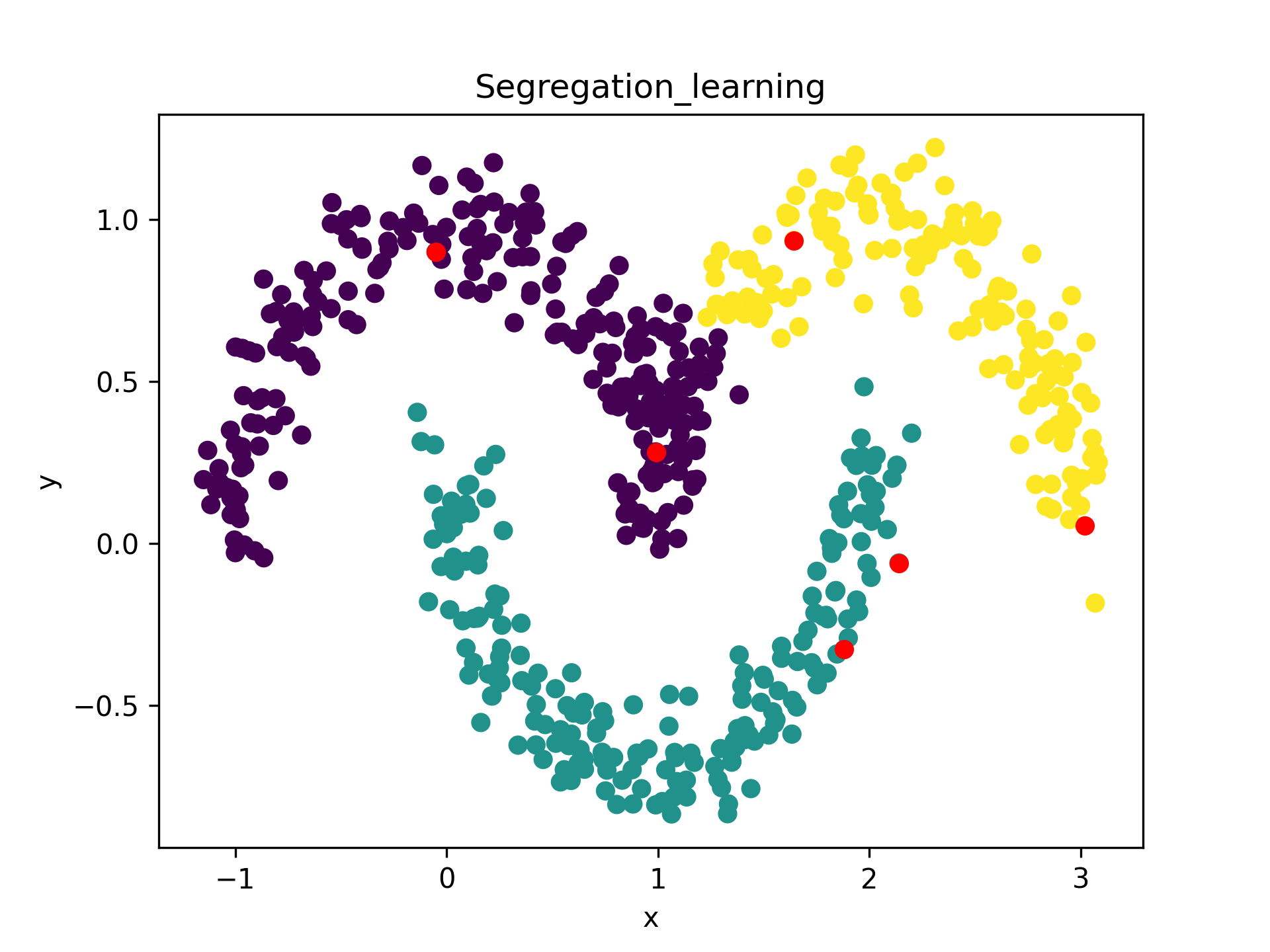
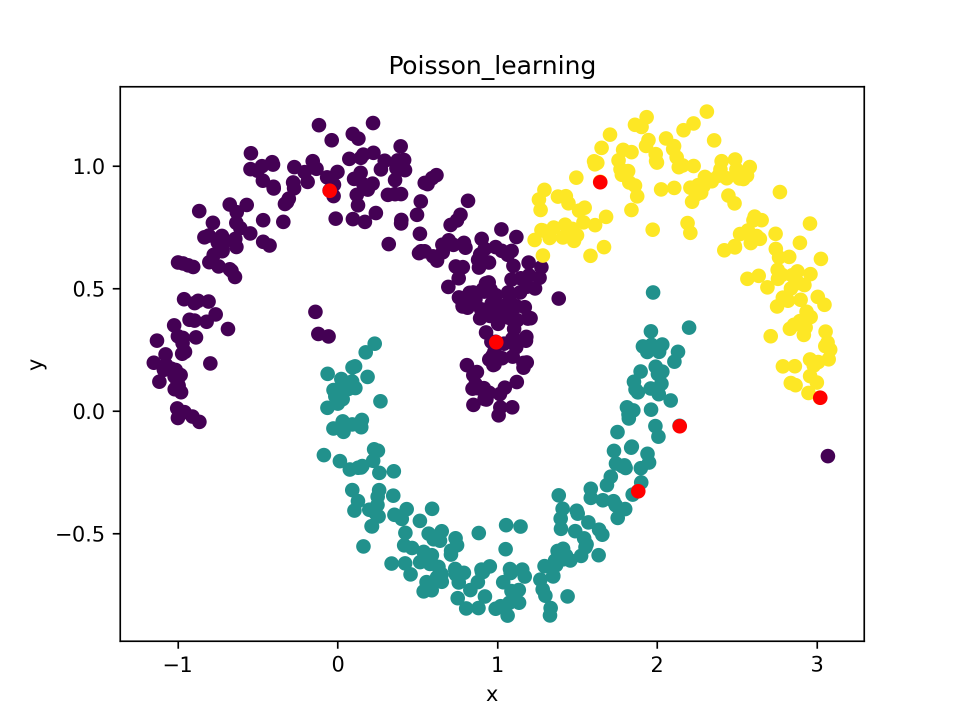
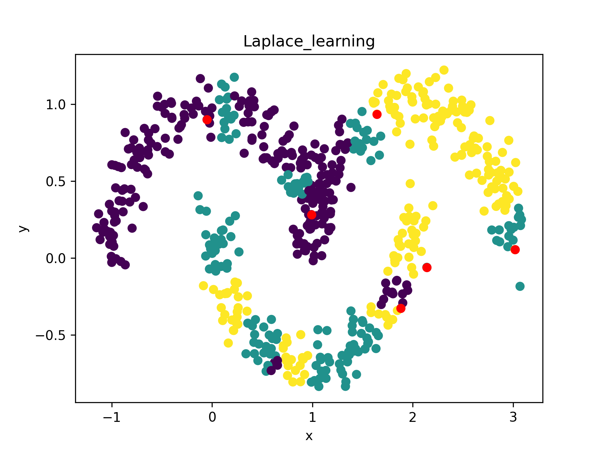
Figure 1. Comparison of Laplace, Poisson and Segregation learning algorithms for 3 classes and initial 2 labels per class.

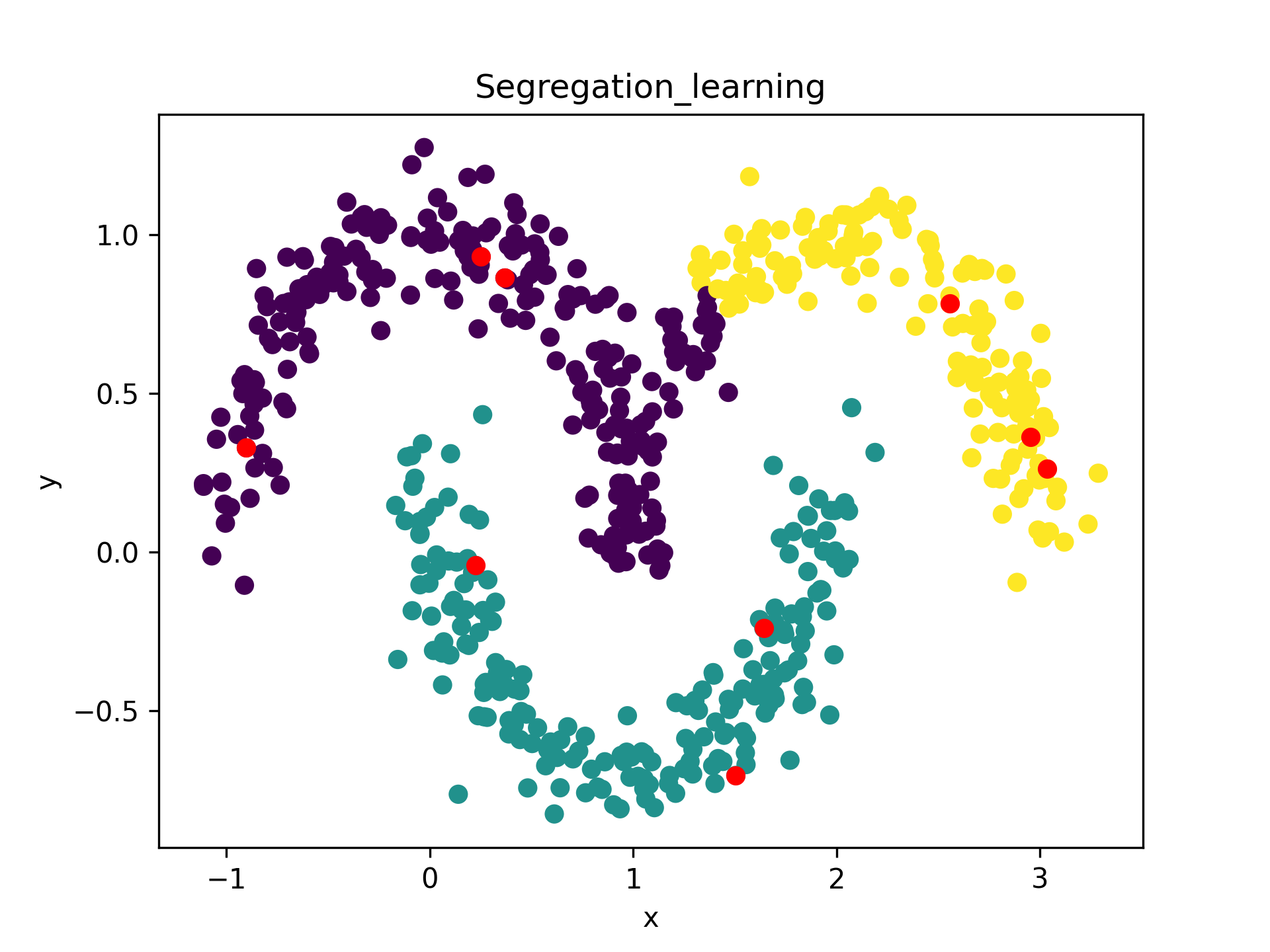
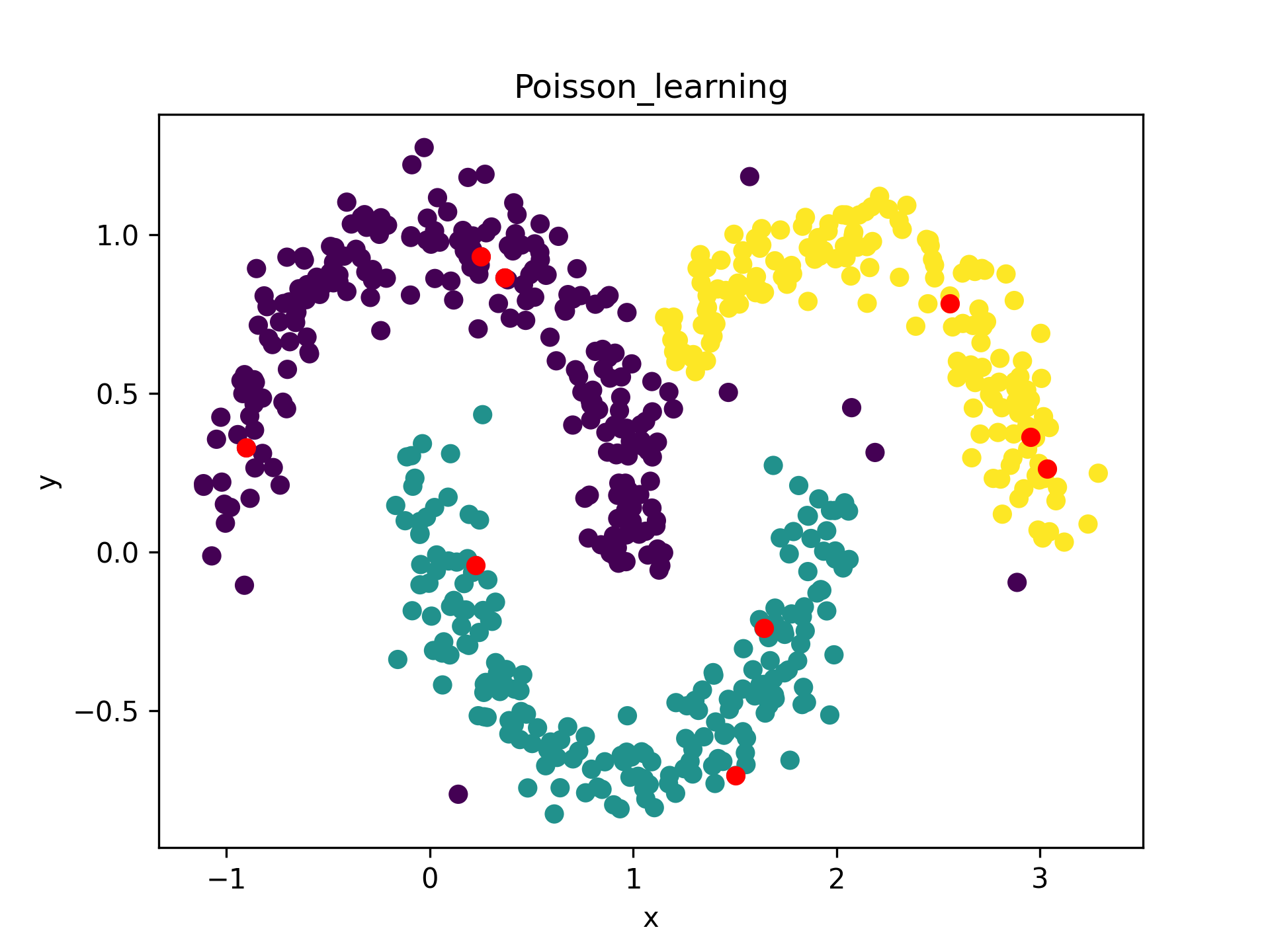
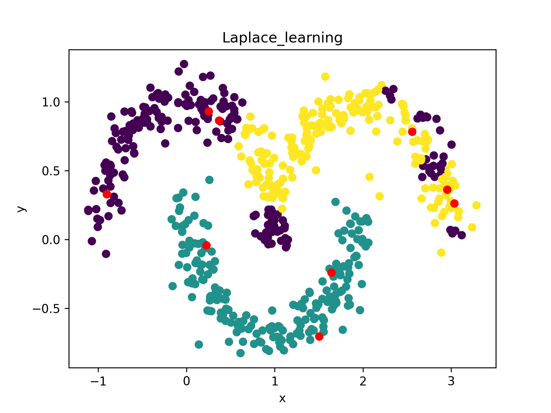
Figure 2. Comparison of Laplace, Poisson and Segregation learning algorithms for 3 classes and initial 3 labels per class.

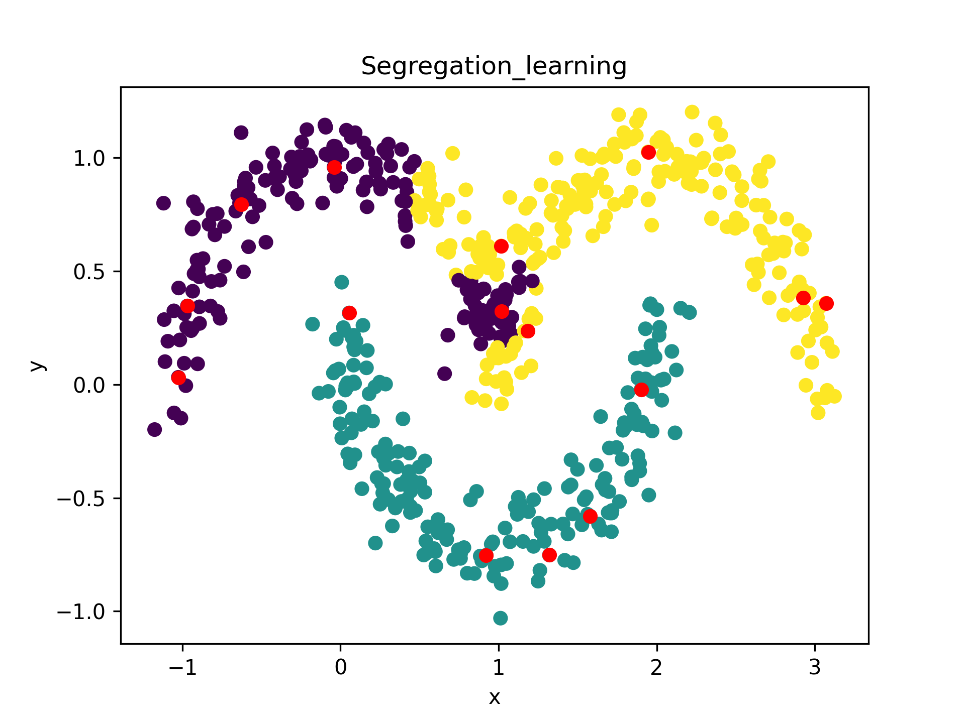
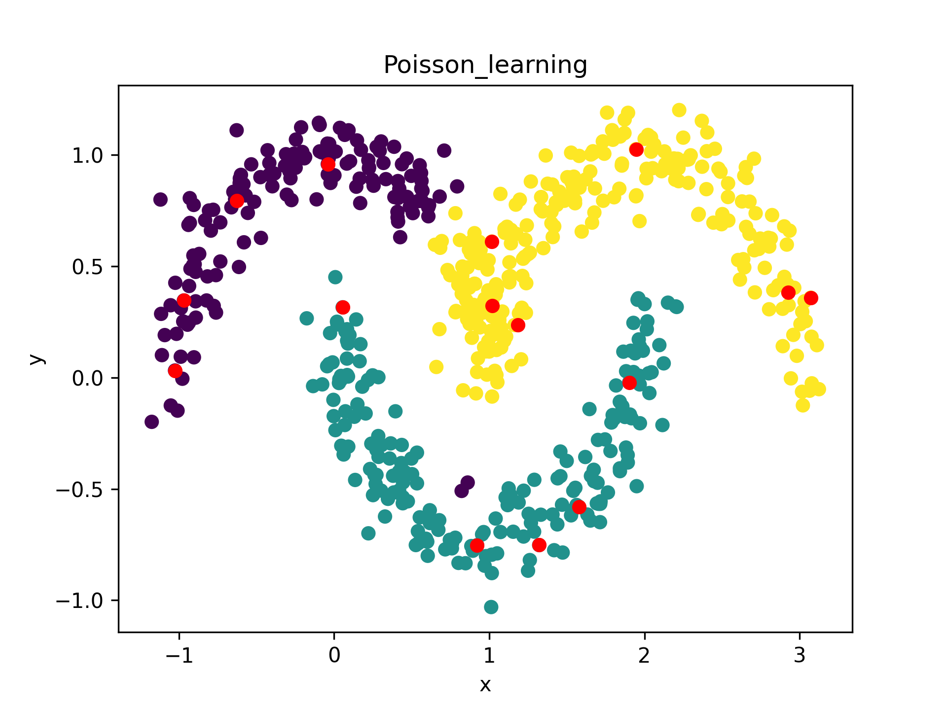
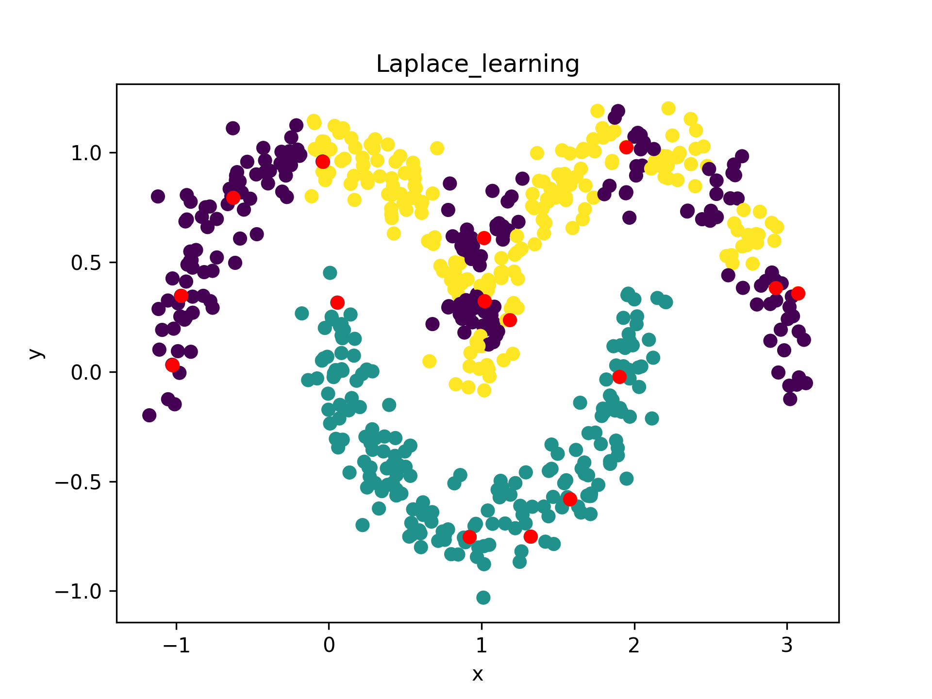
Figure 3. Comparison of Laplace, Poisson and Segregation learning algorithms for 3 classes and initial 5 labels per class.

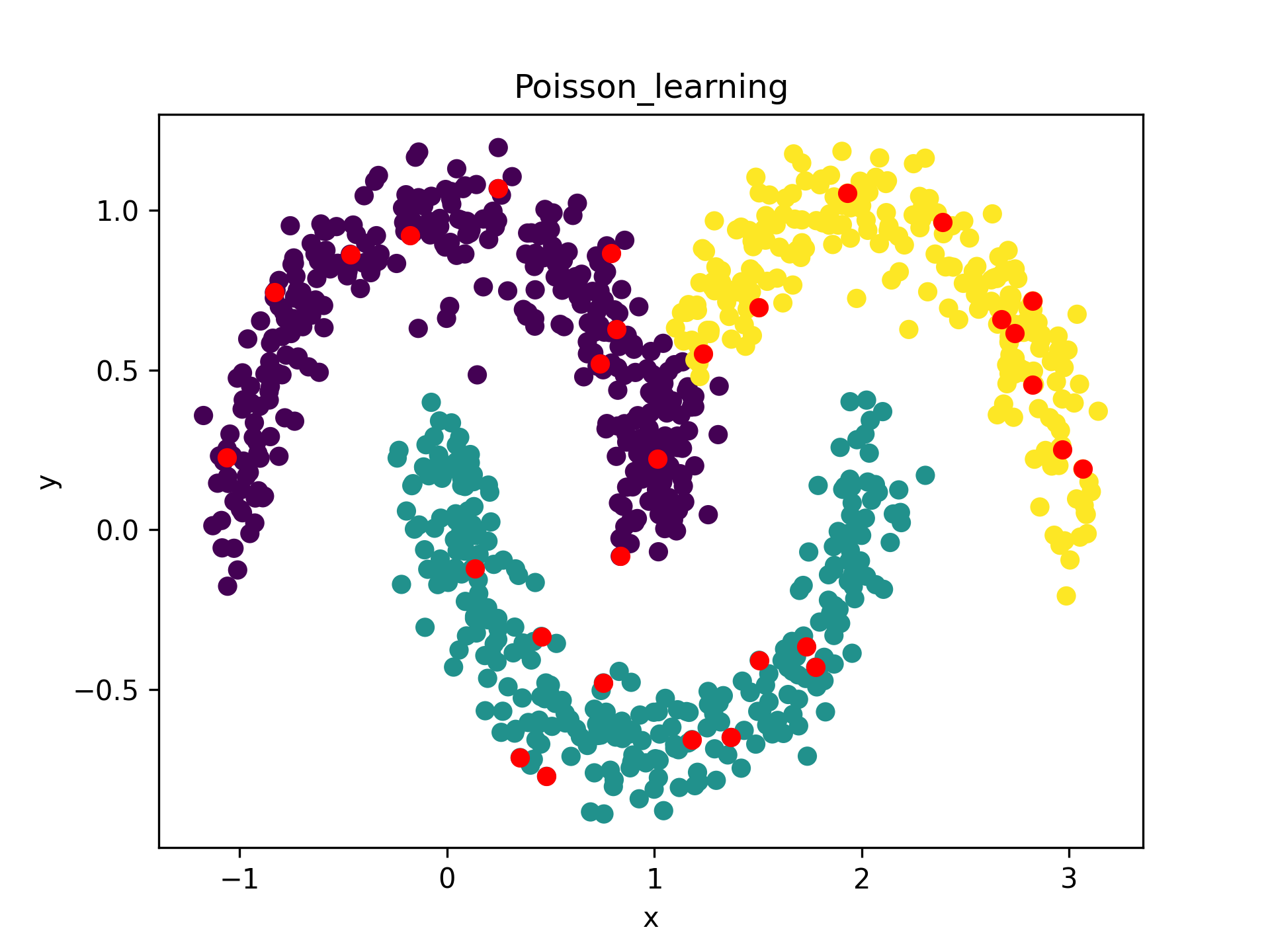
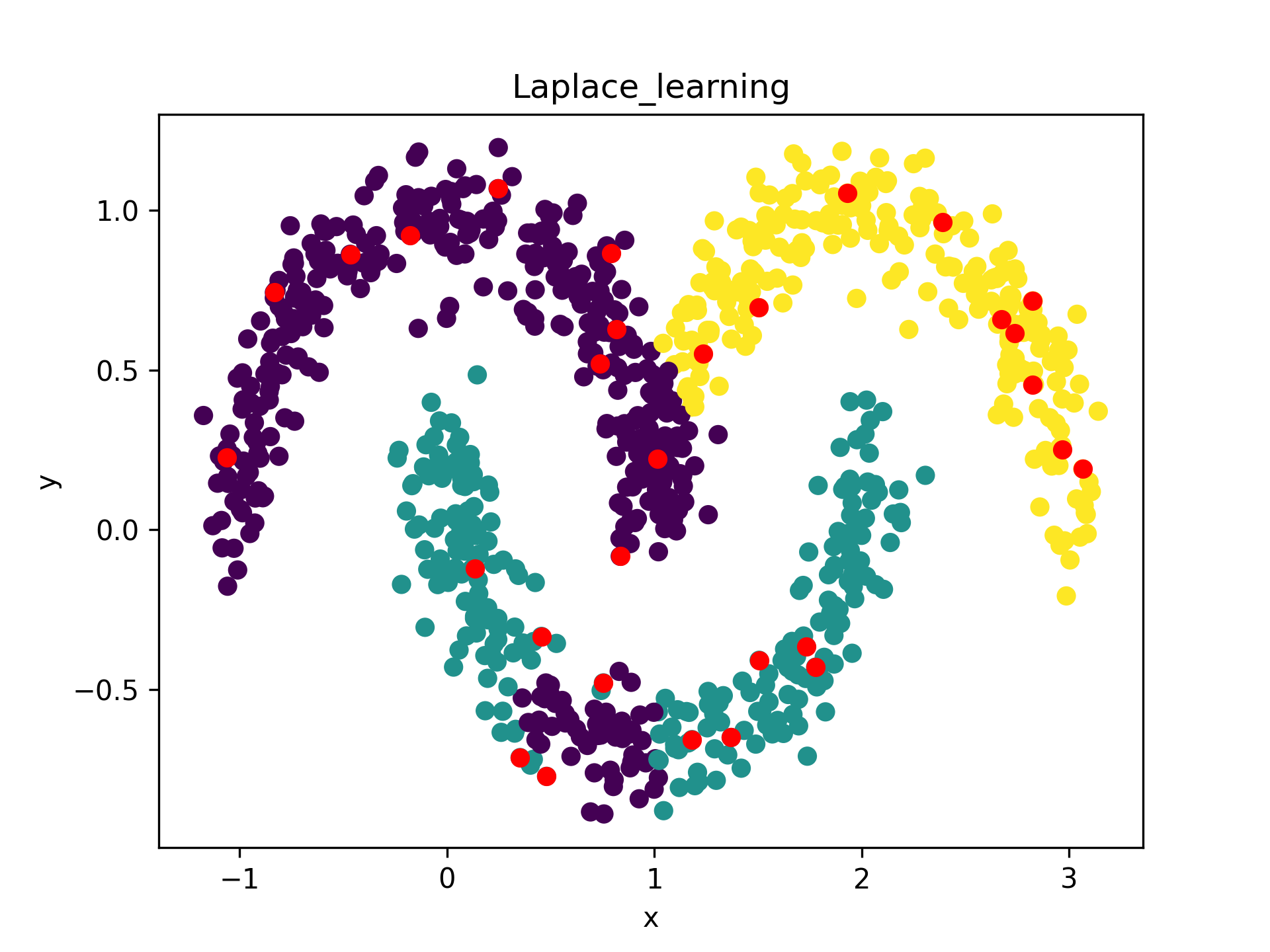
Figure 4. Comparison of Laplace, Poisson and Segregation learning algorithms for 3 classes and initial 10 labels per class.

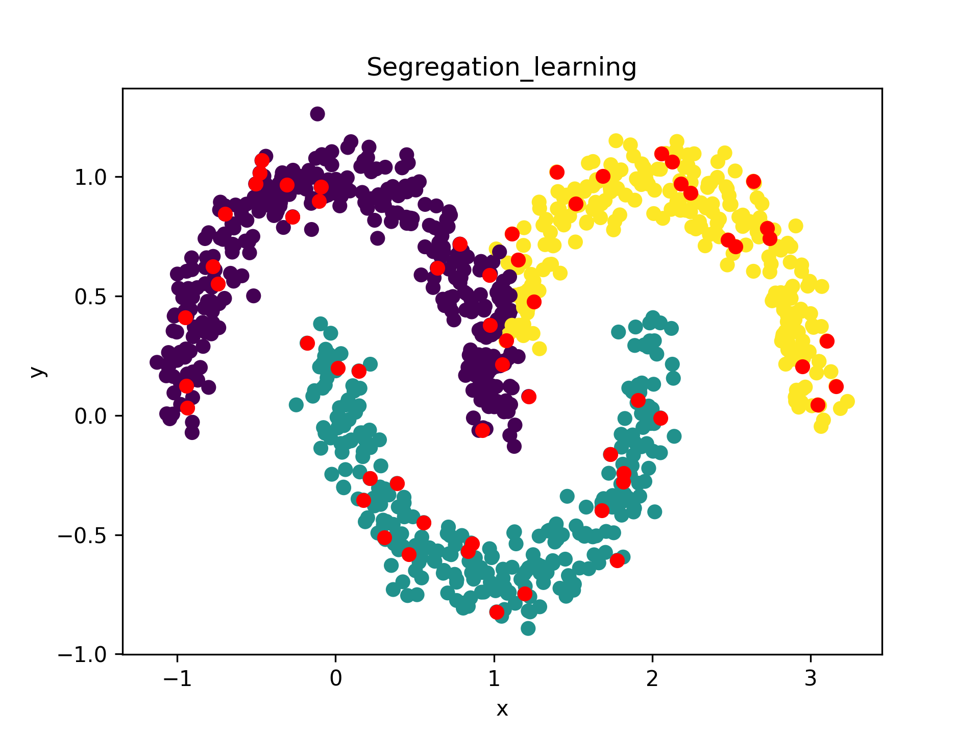
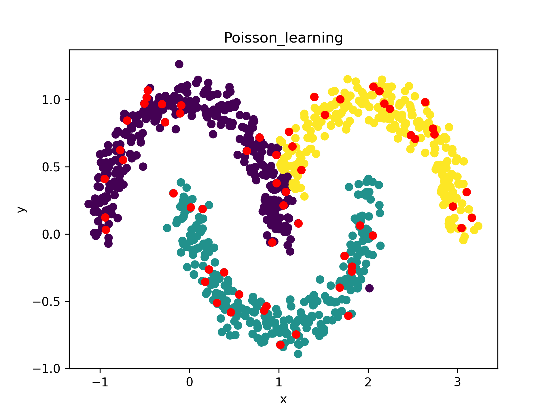
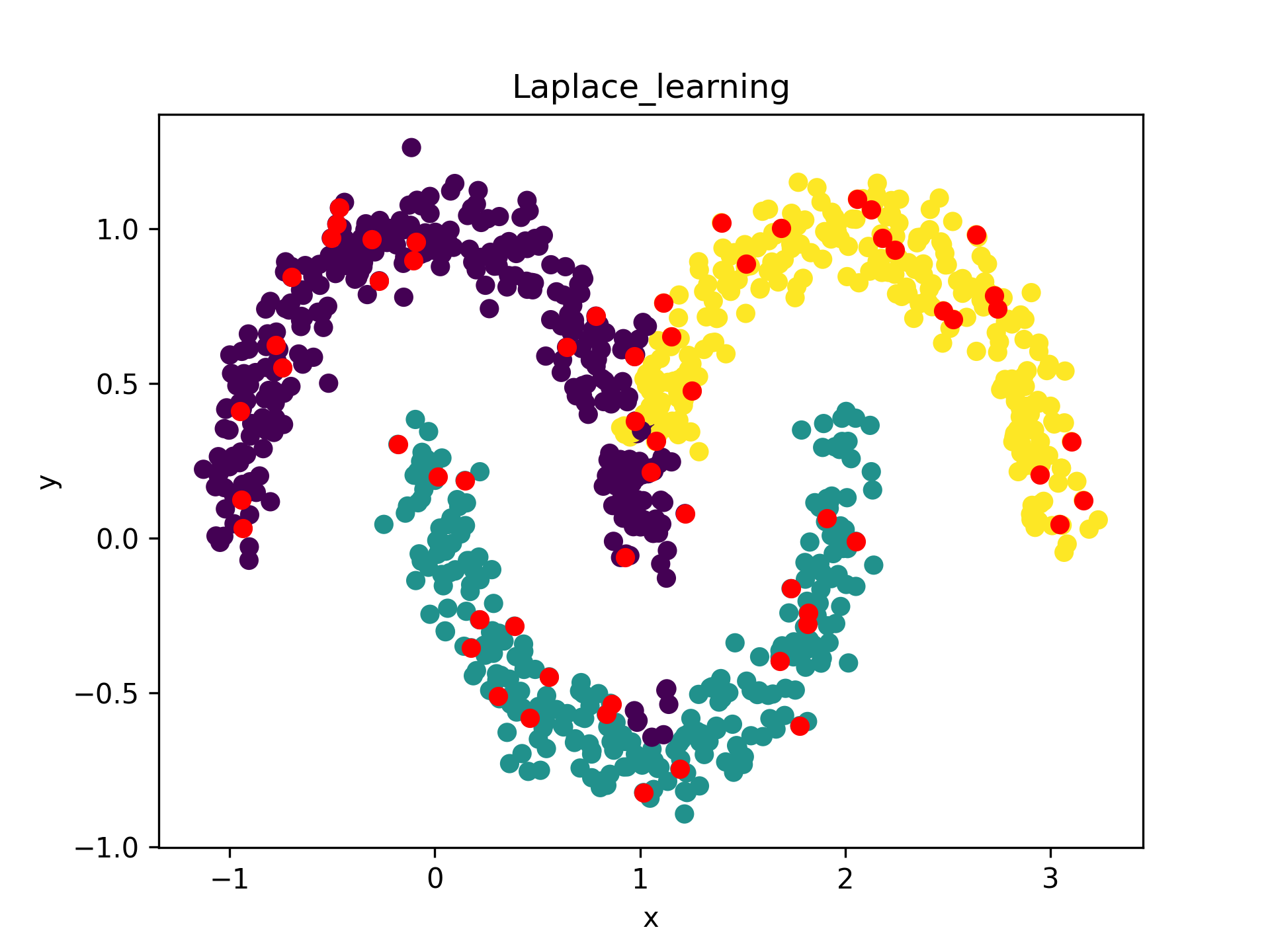
Figure 5. Comparison of Laplace, Poisson and Segregation learning algorithms for 3 classes and initial 20 labels per class.

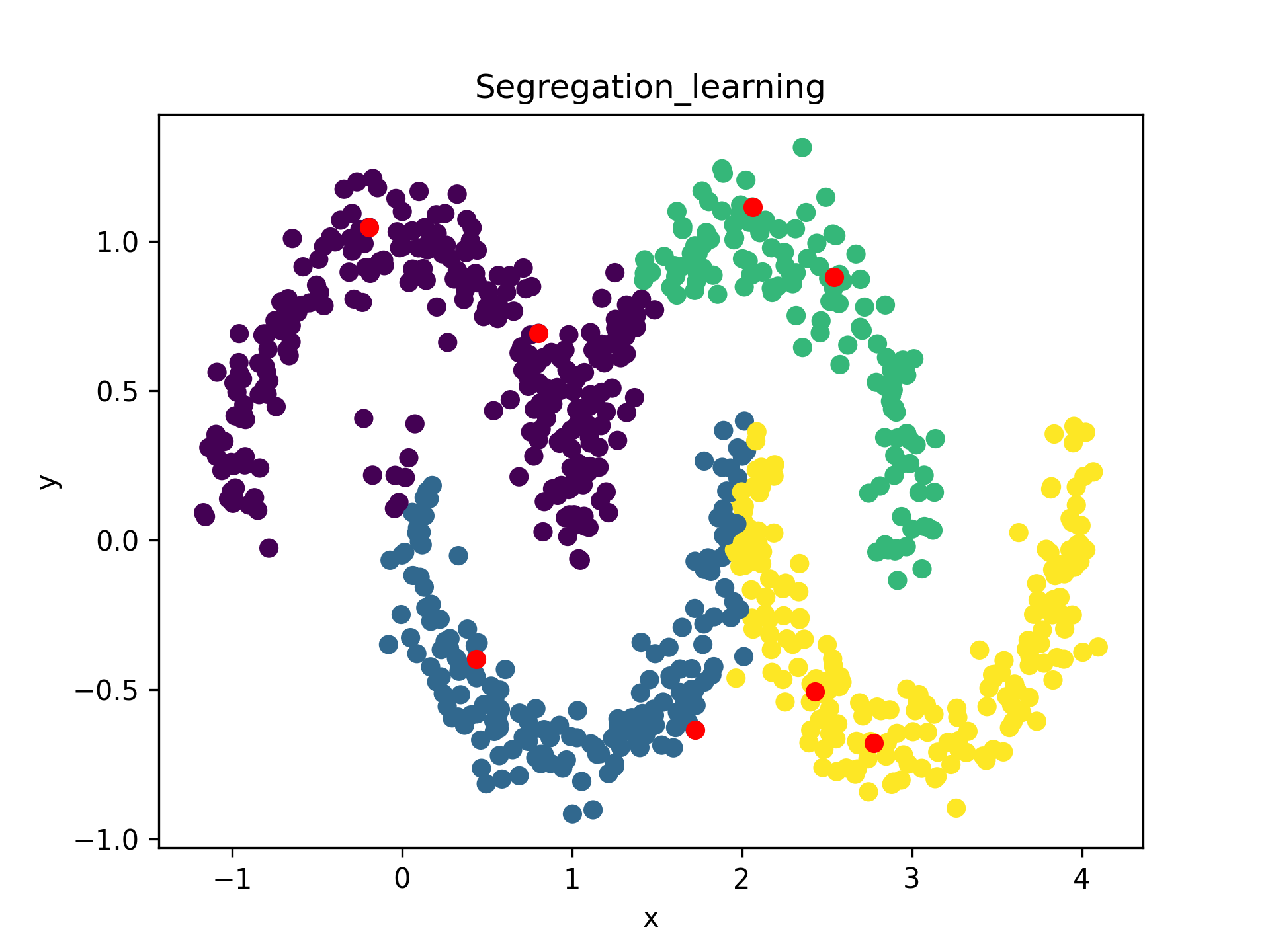
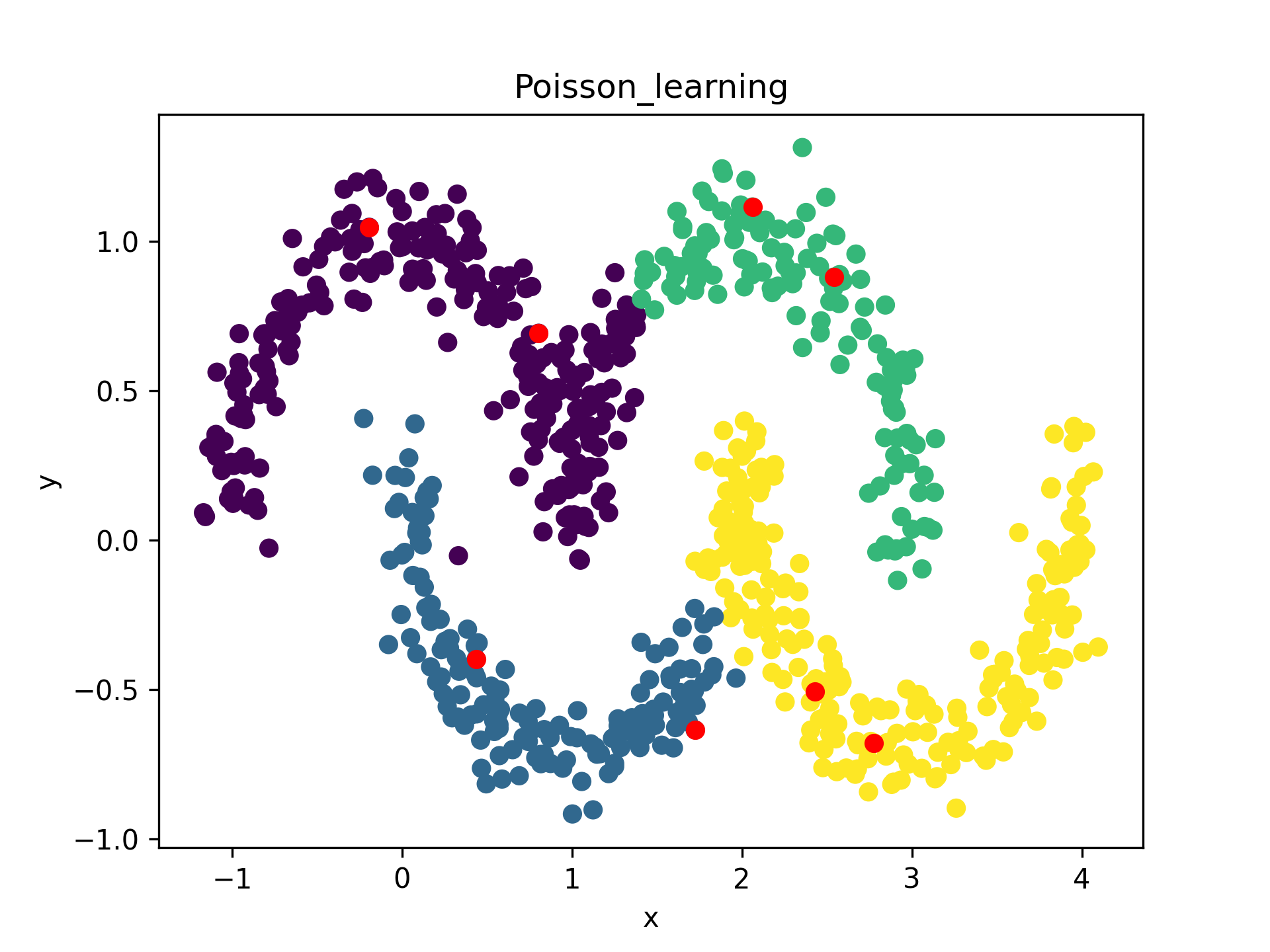
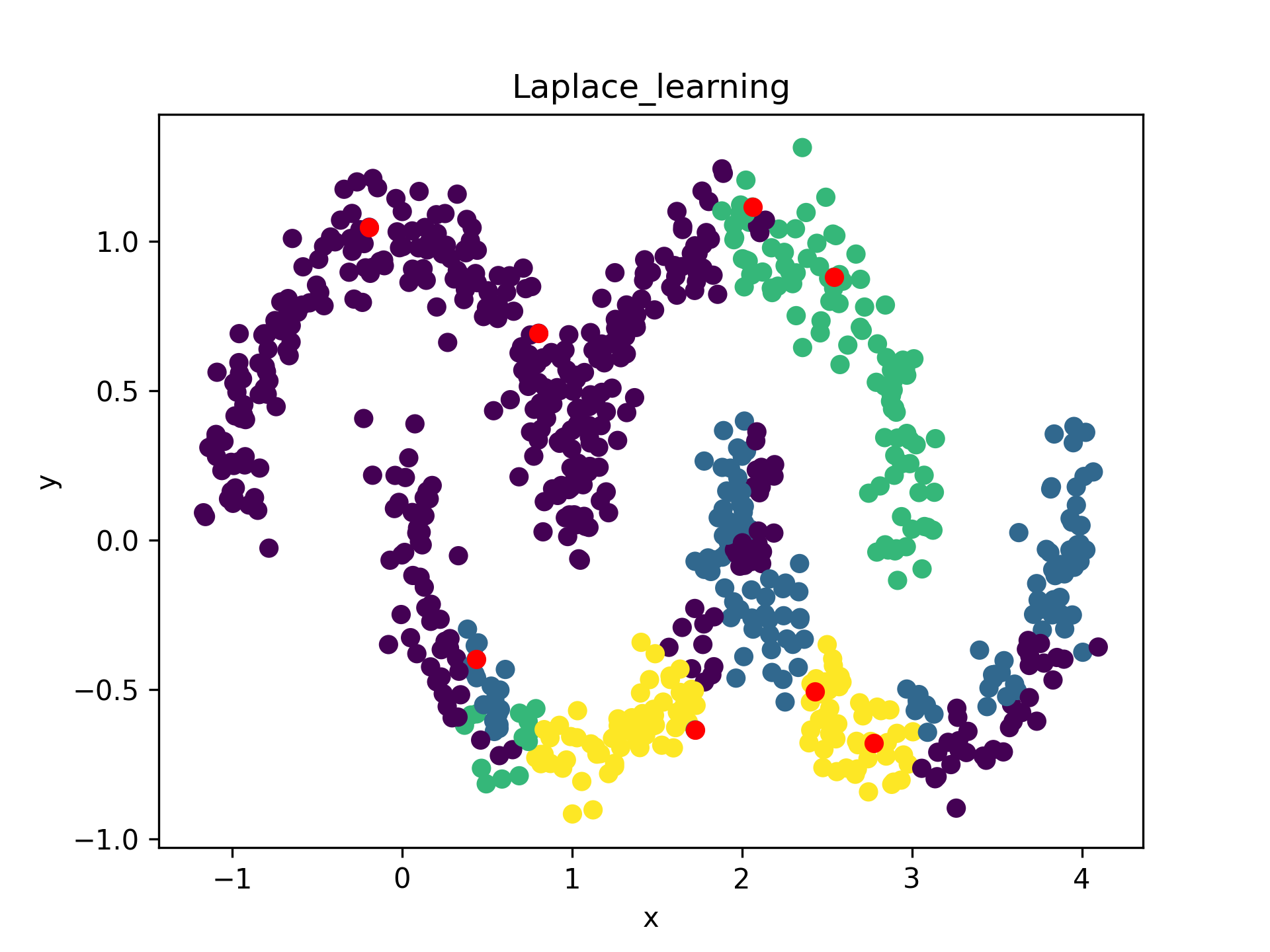
Figure 6. Comparison of Laplace, Poisson and Segregation learning algorithms for 4 classes and initial 2 labels per class.

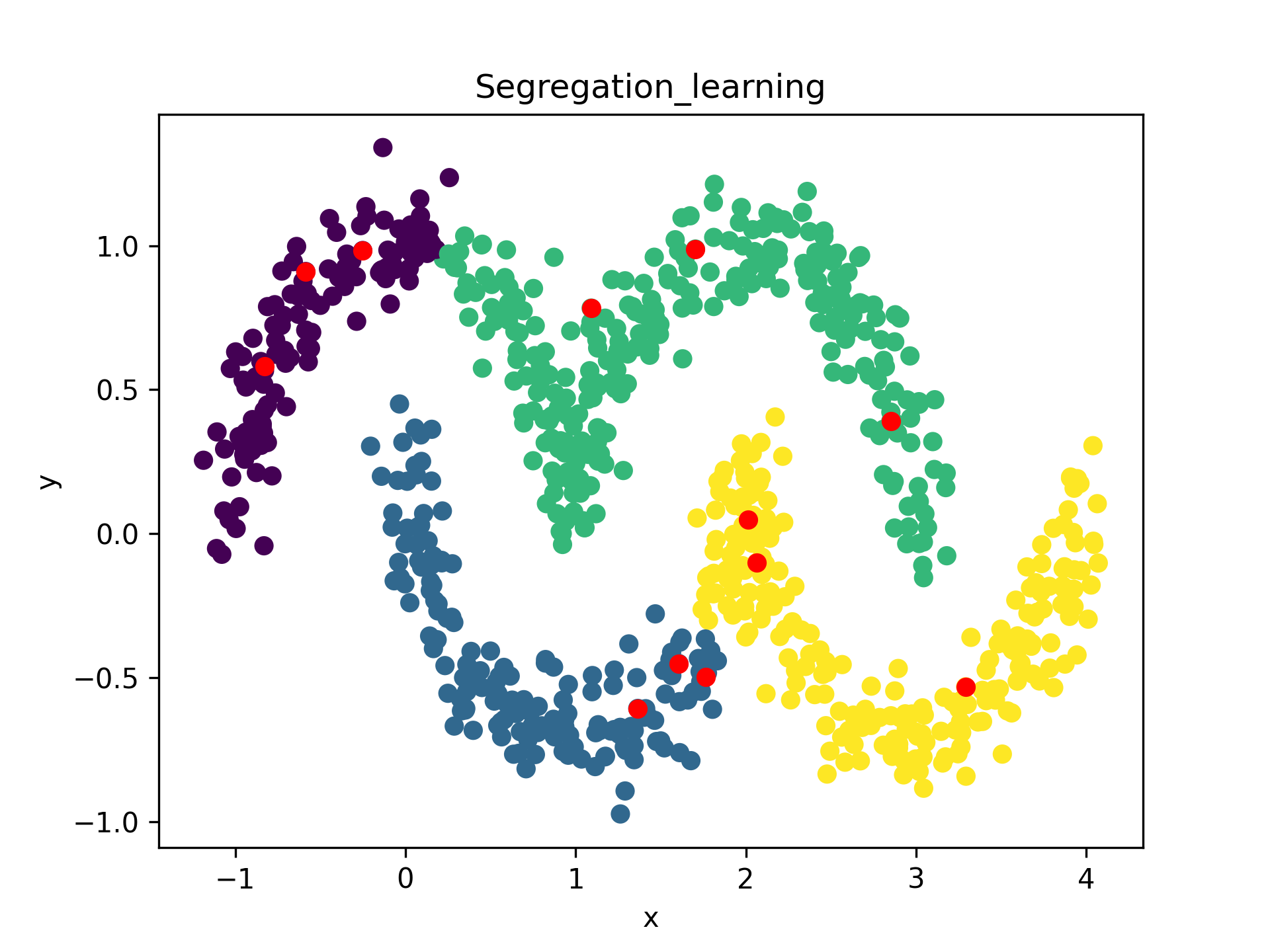
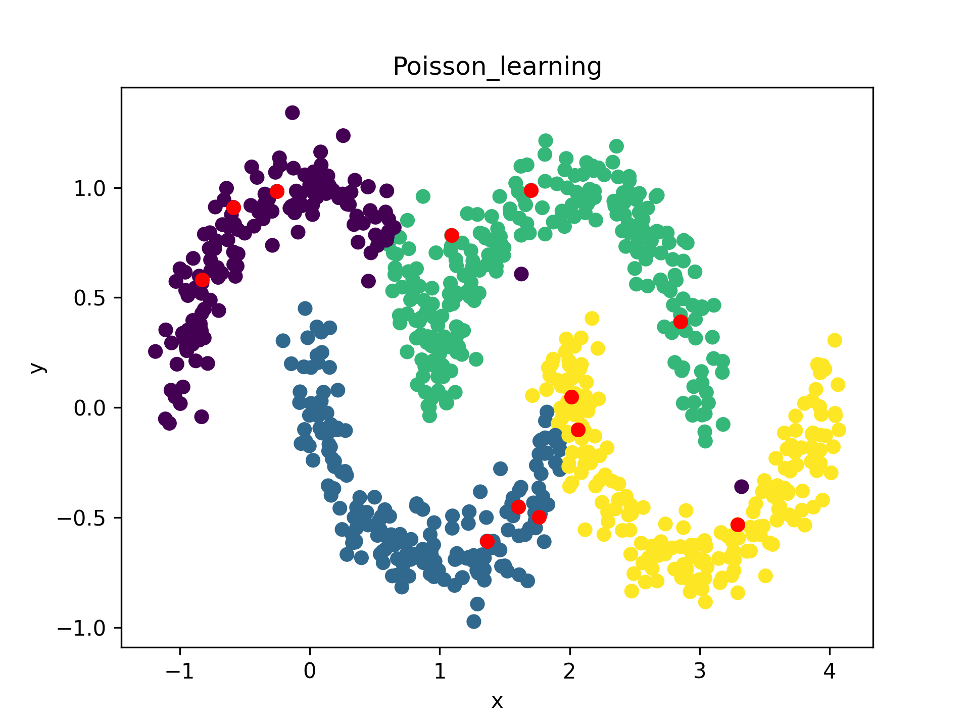
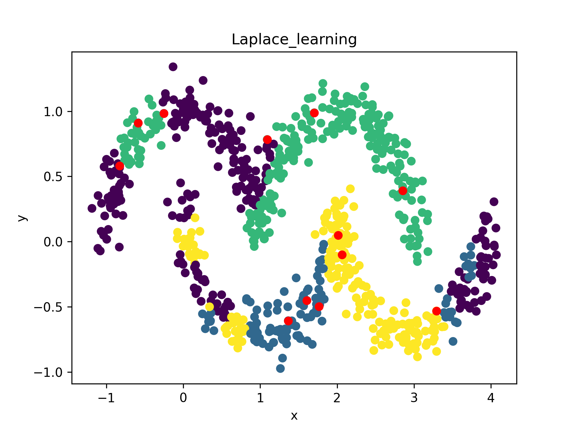
Figure 7. Comparison of Laplace, Poisson and Segregation learning algorithms for 4 classes and initial 3 labels per class.

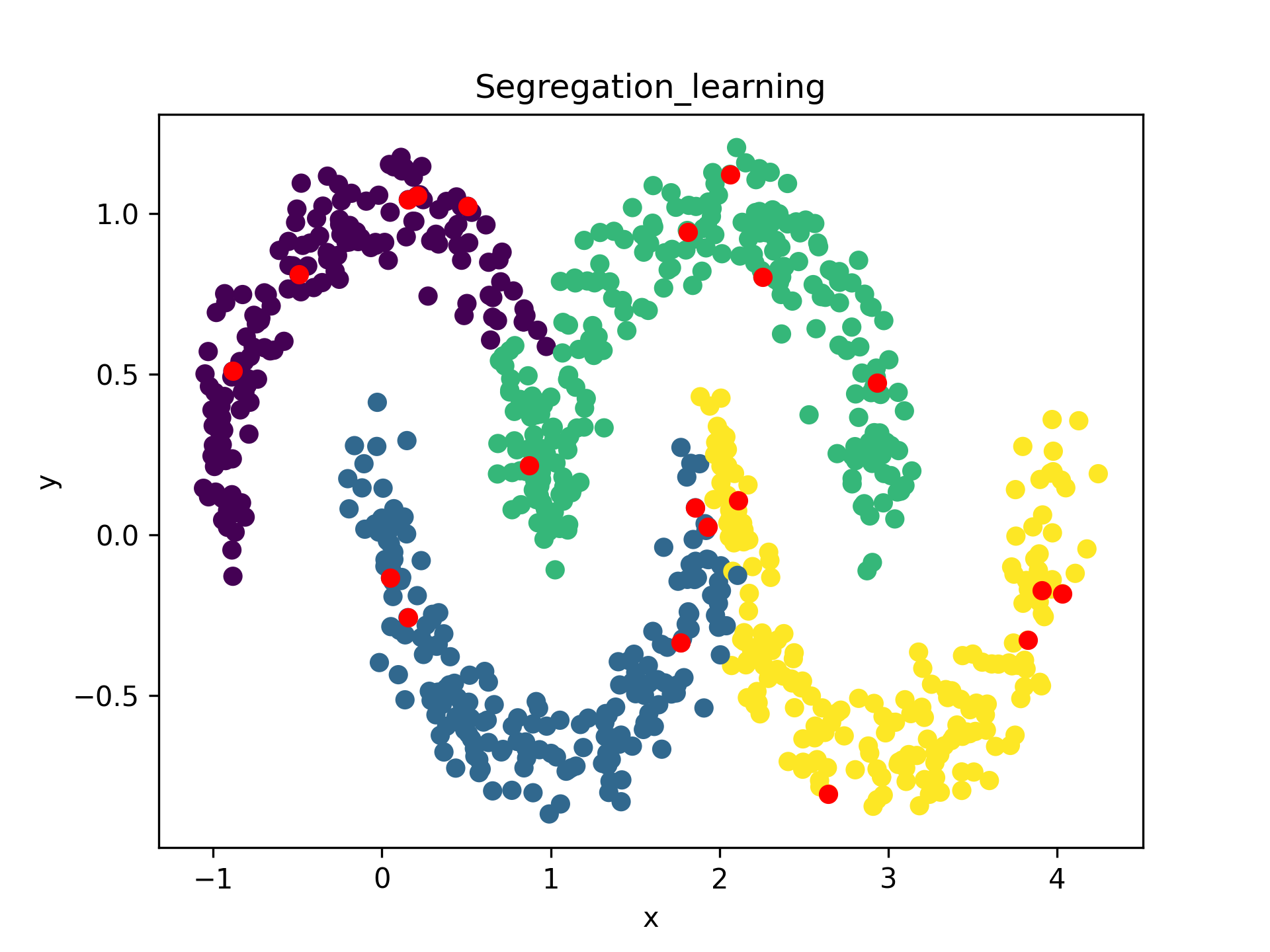
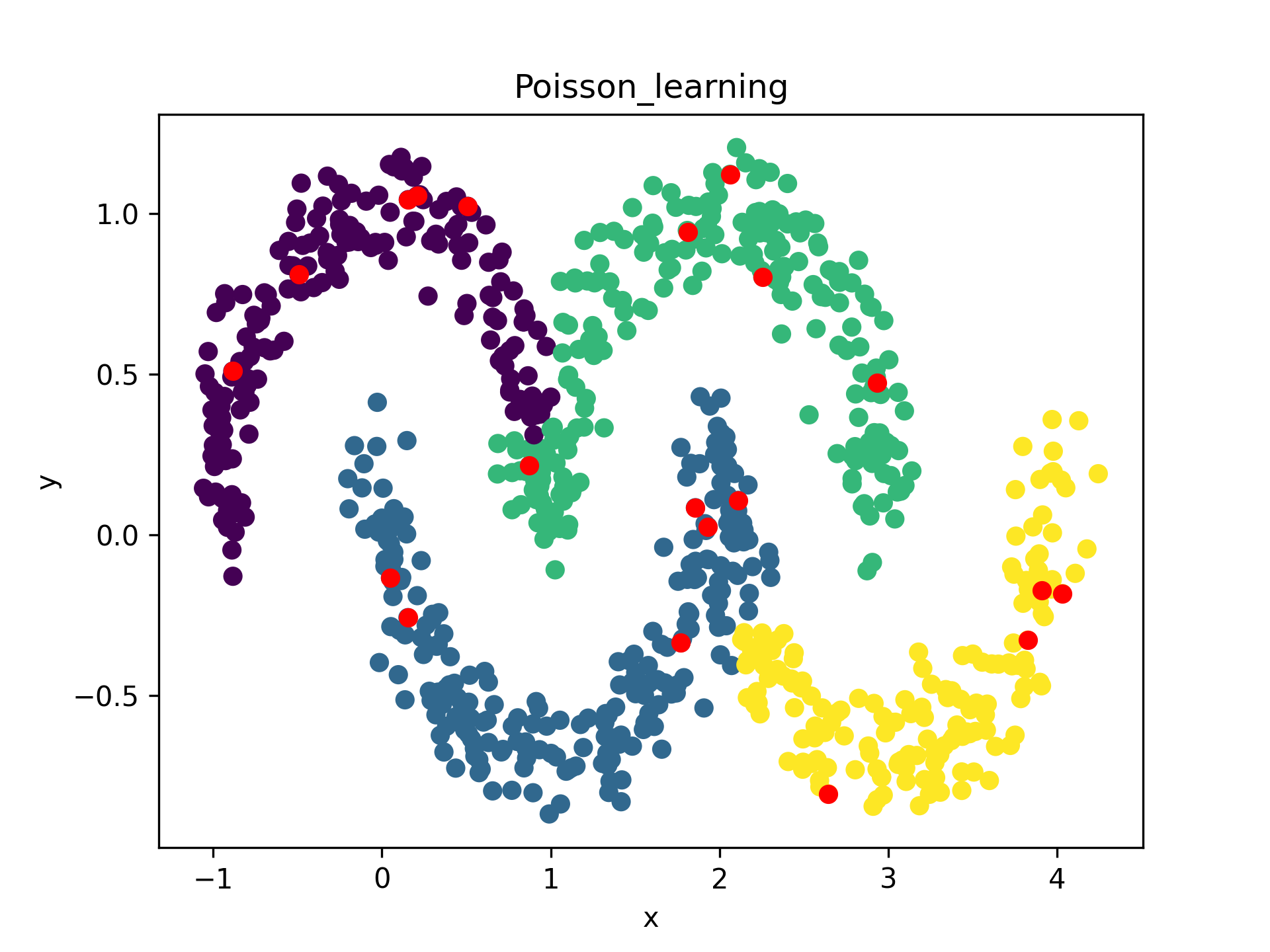
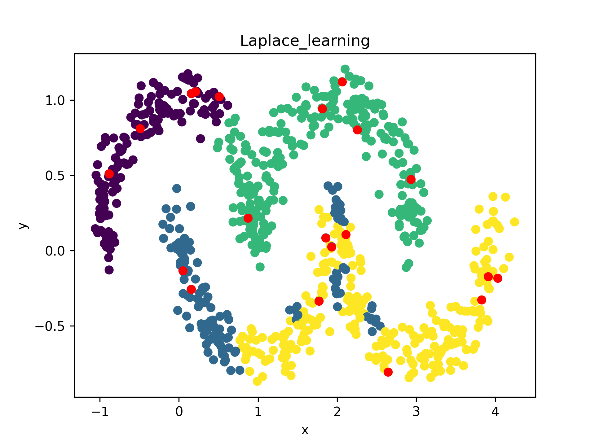
Figure 8. Comparison of Laplace, Poisson and Segregation learning algorithms for 4 classes and initial 5 labels per class.

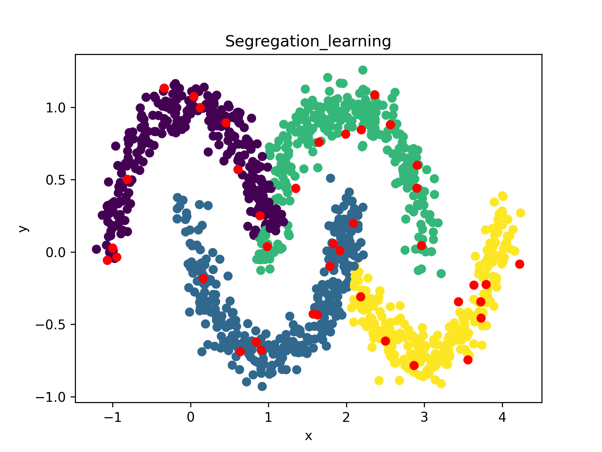
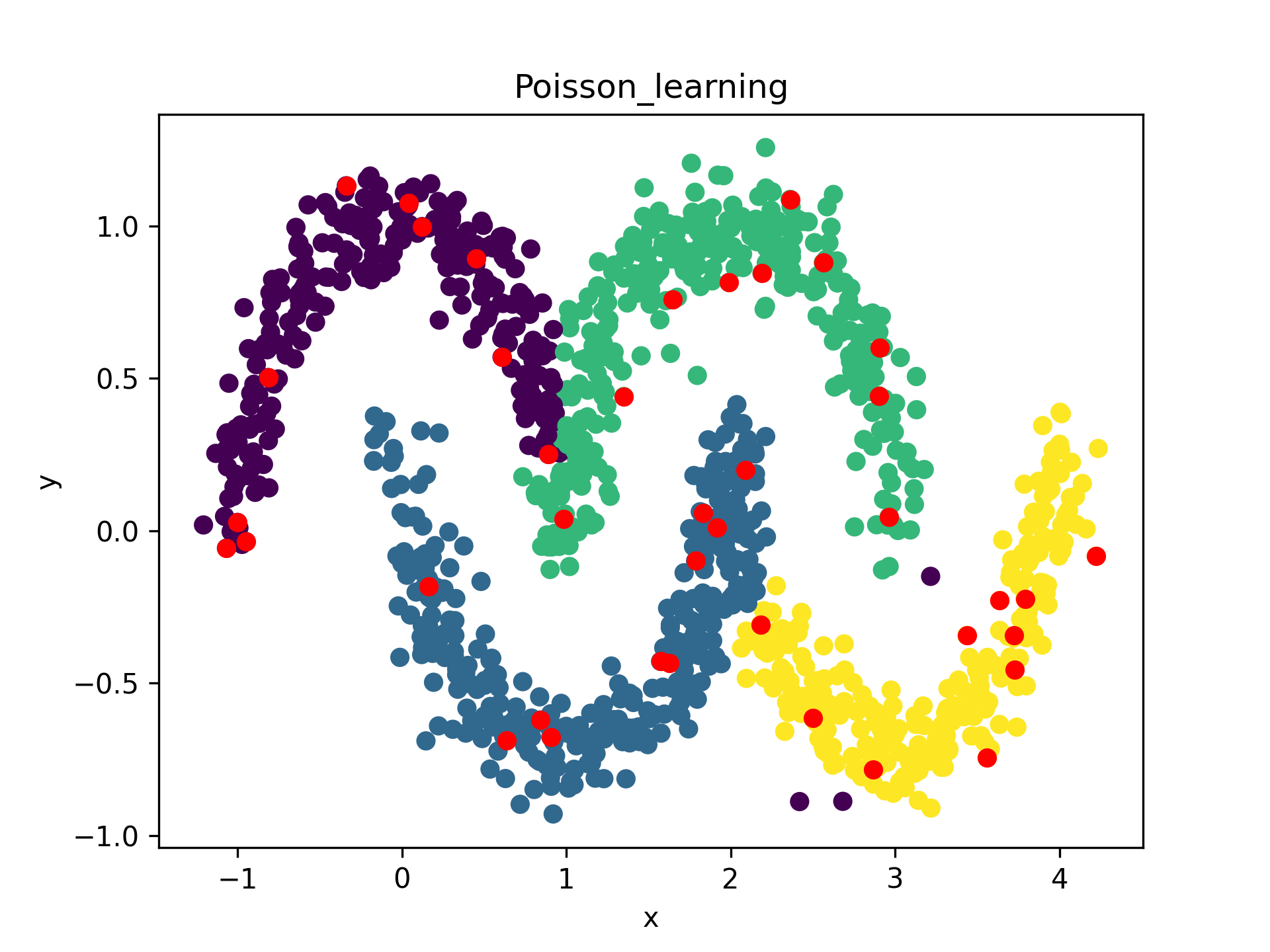
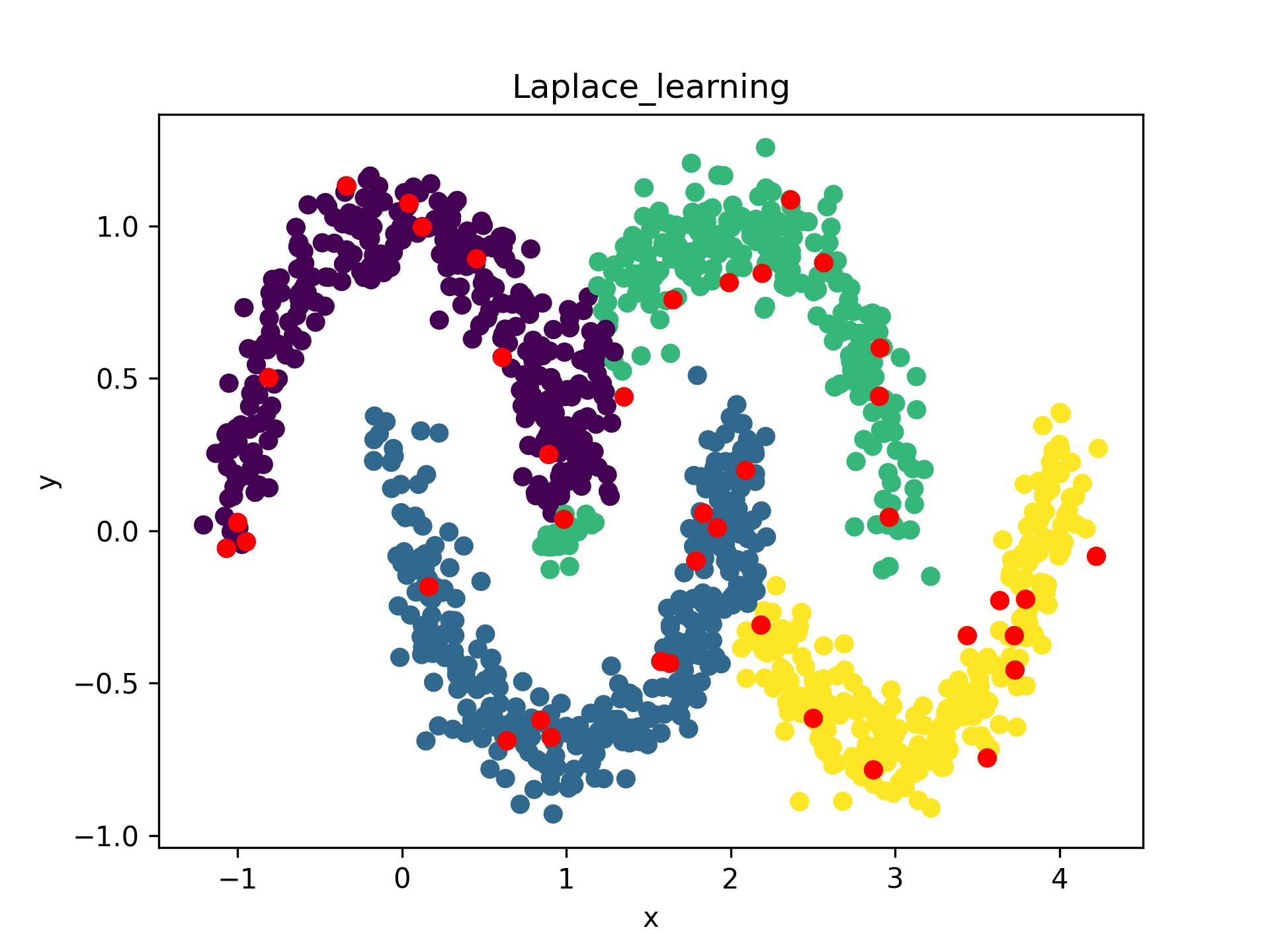
Figure 9. Comparison of Laplace, Poisson and Segregation learning algorithms for 4 classes and initial 10 labels per class.

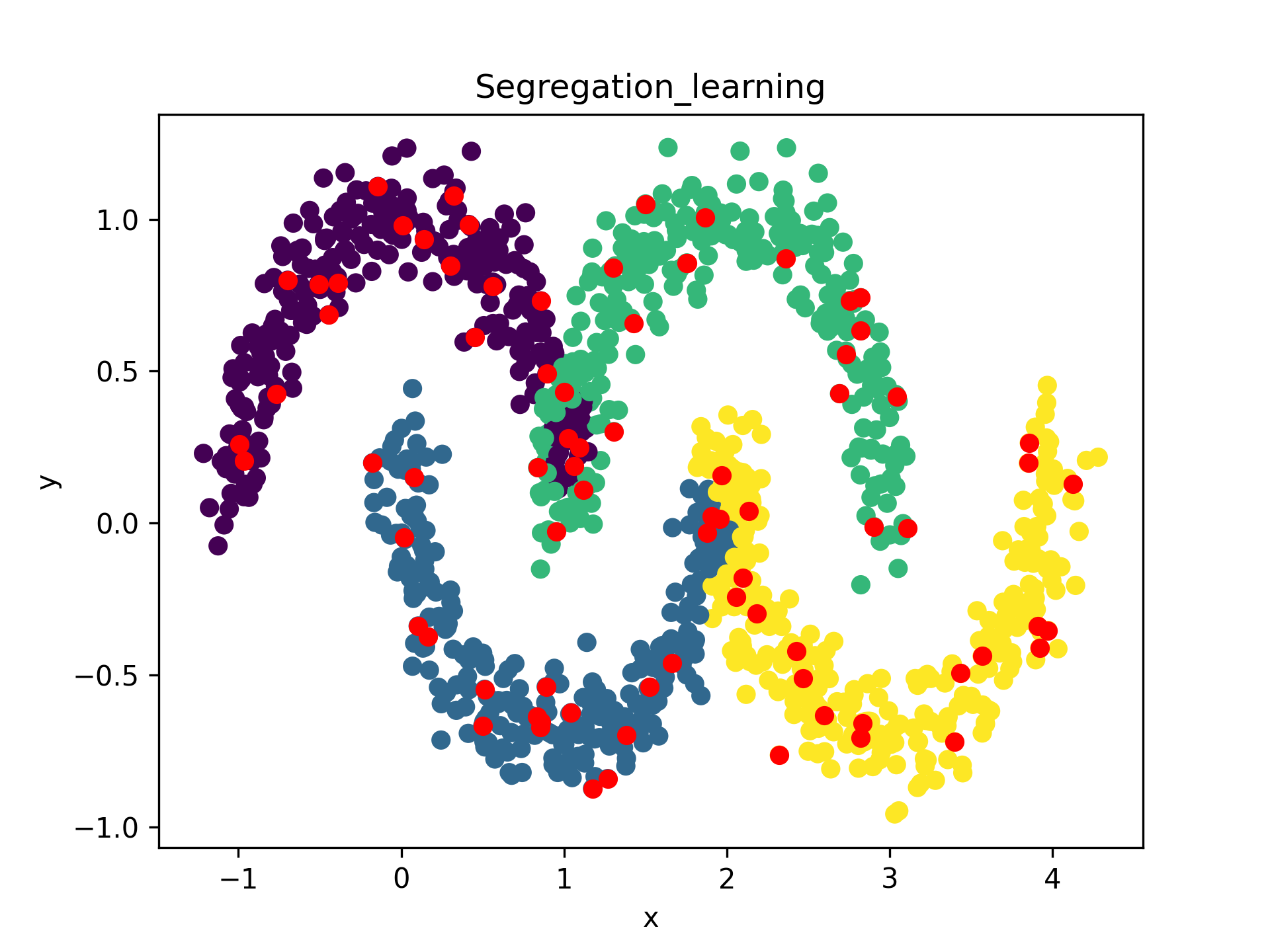
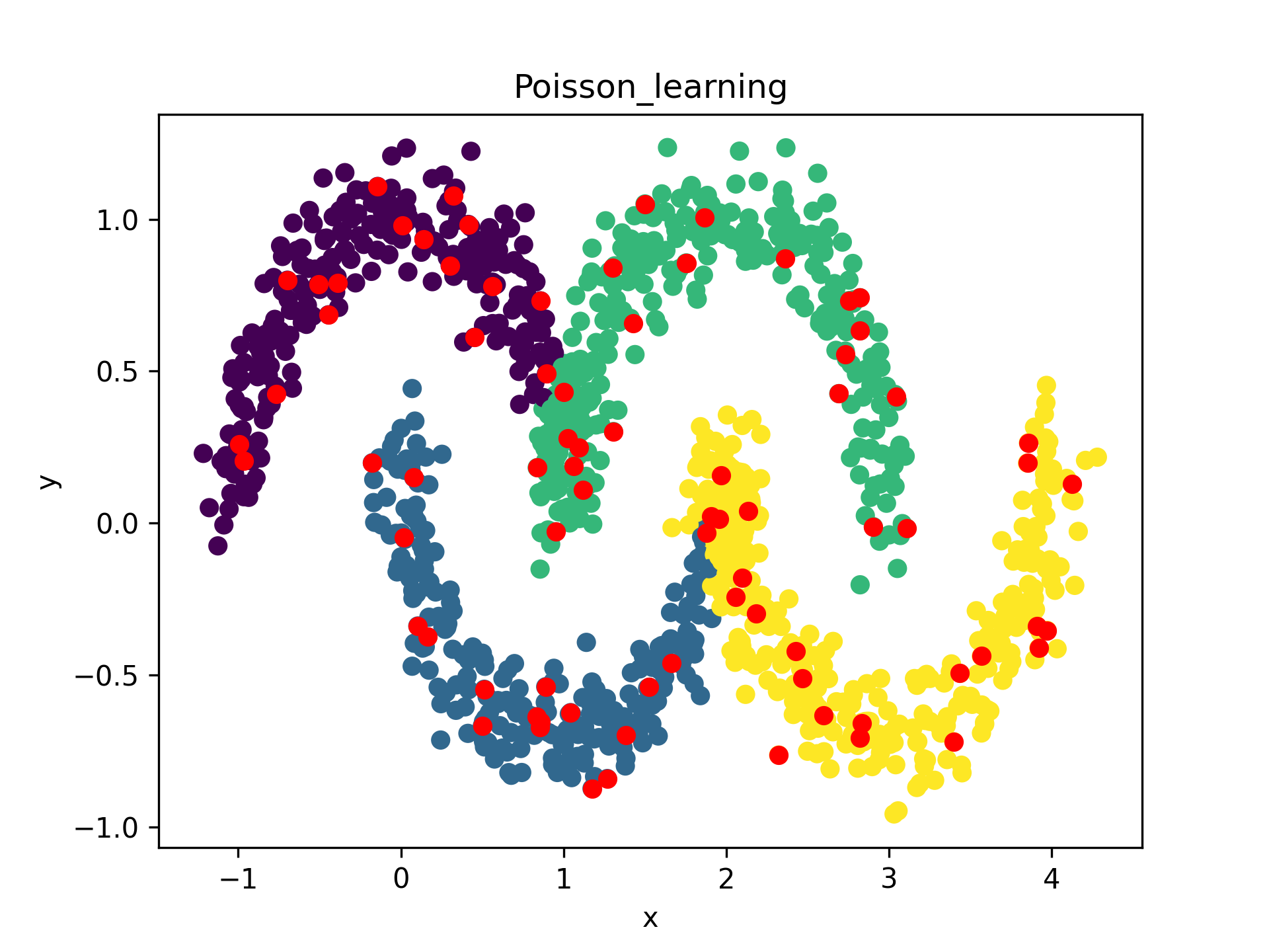
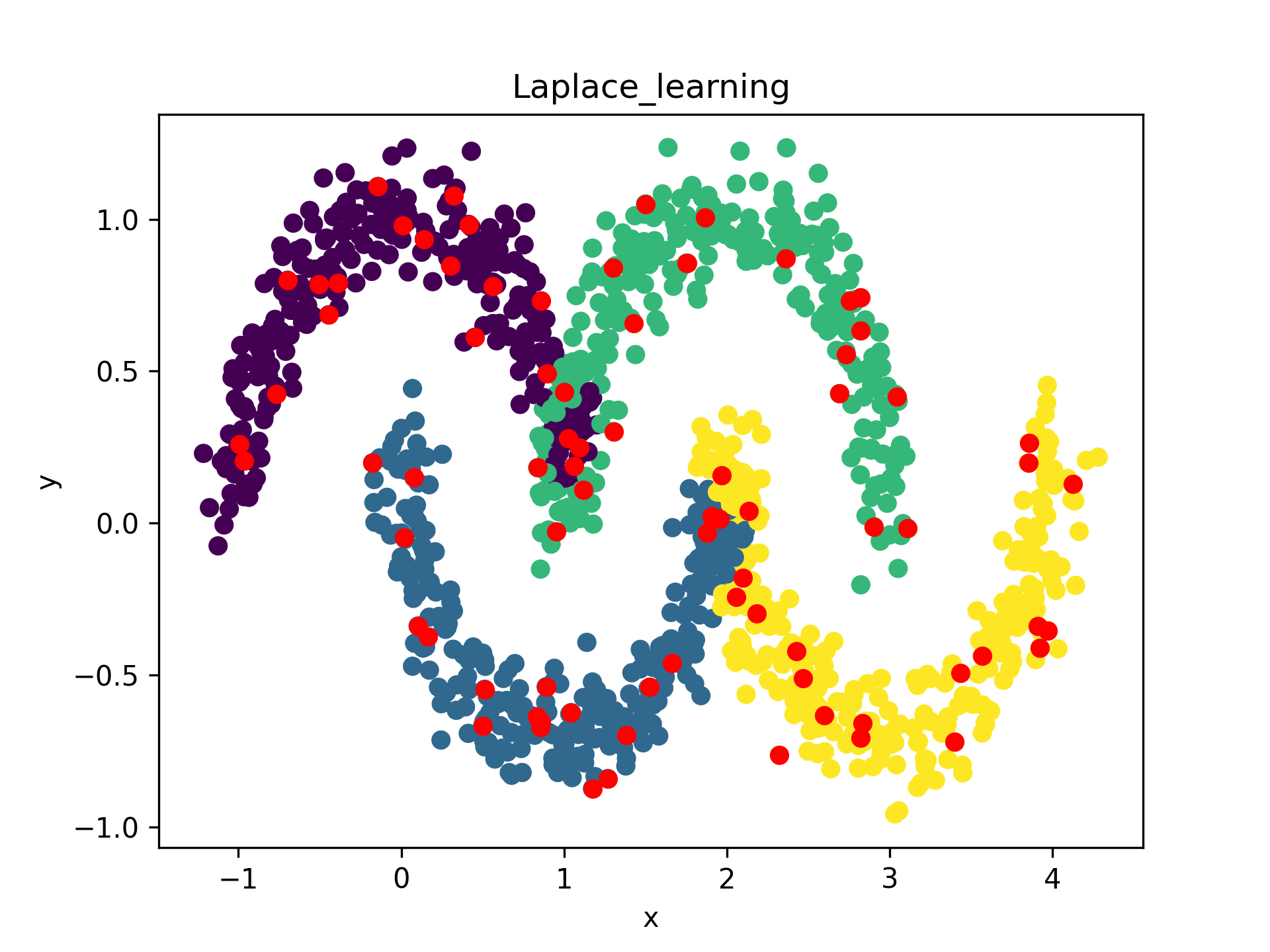
Figure 10. Comparison of Laplace, Poisson and Segregation learning algorithms for 4 classes and initial 20 labels per class.

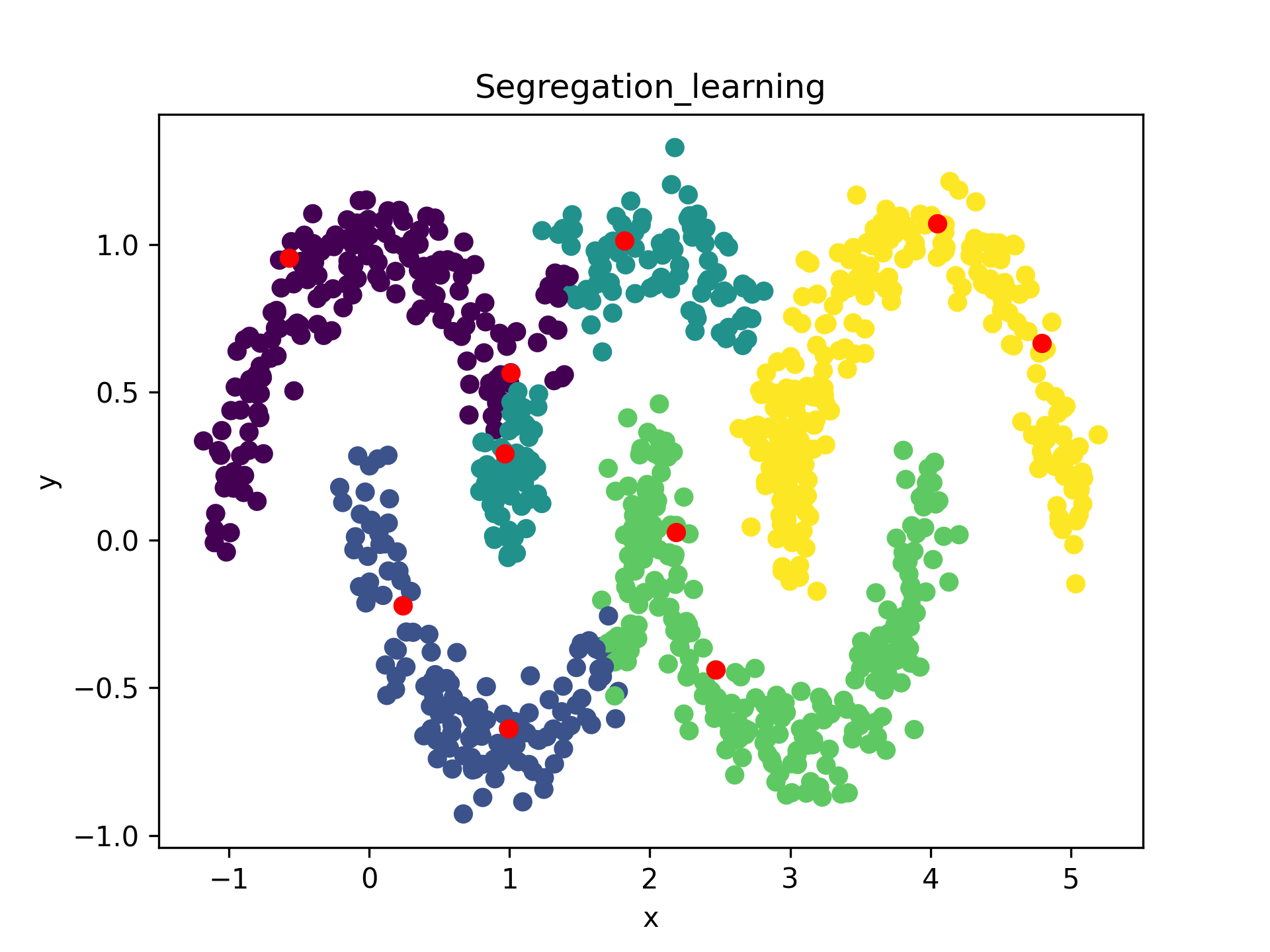
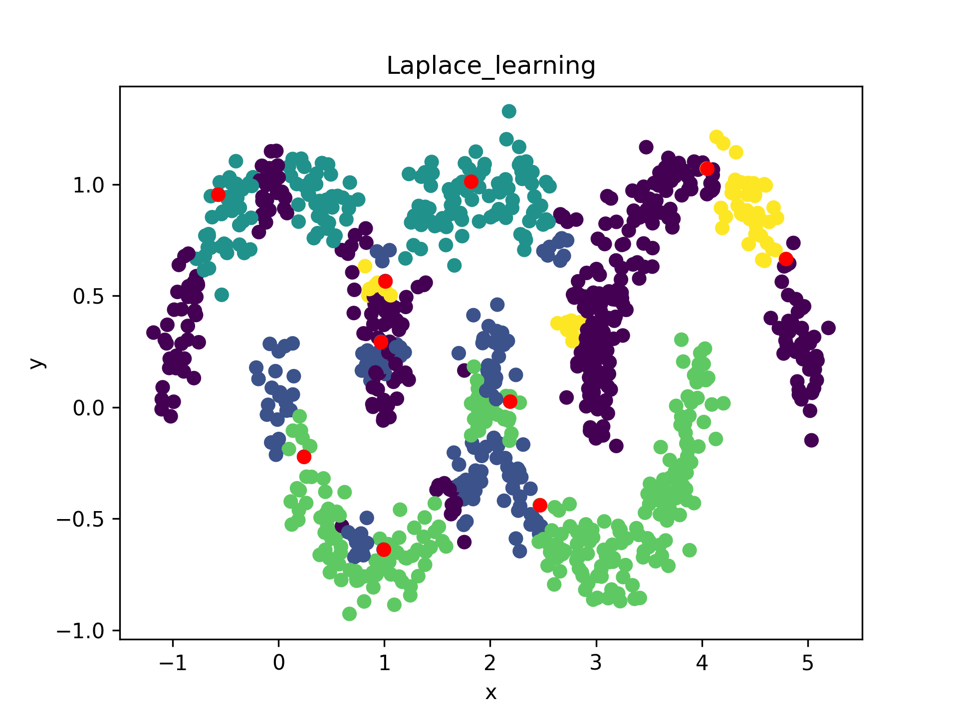
Figure 11. Comparison of Laplace, Poisson and Segregation learning algorithms for 5 classes and initial 2 labels per class.

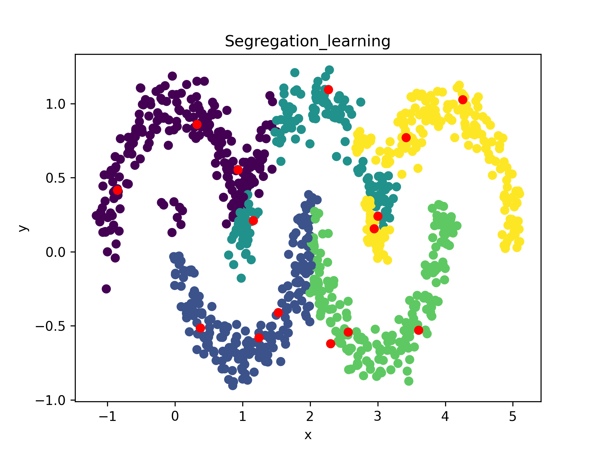
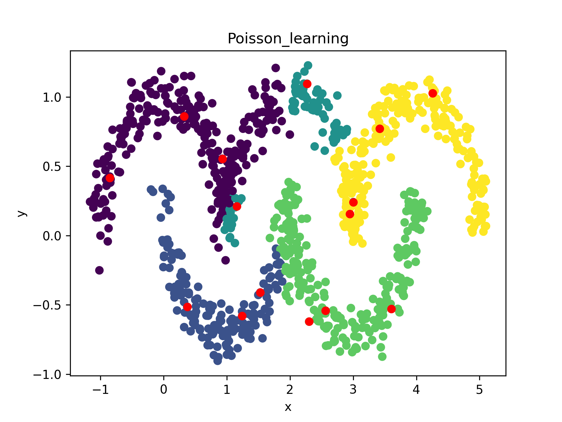
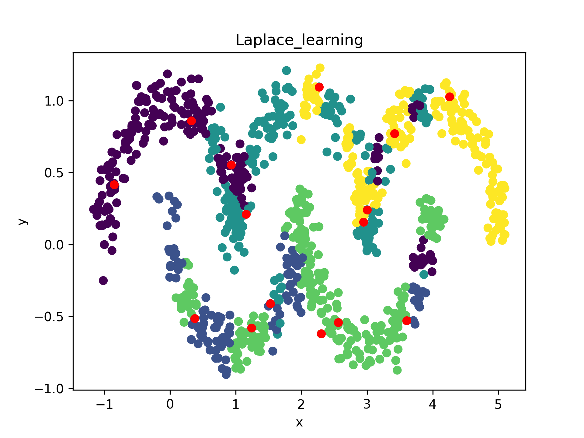
Figure 12. Comparison of Laplace, Poisson and Segregation learning algorithms for 5 classes and initial 3 labels per class.

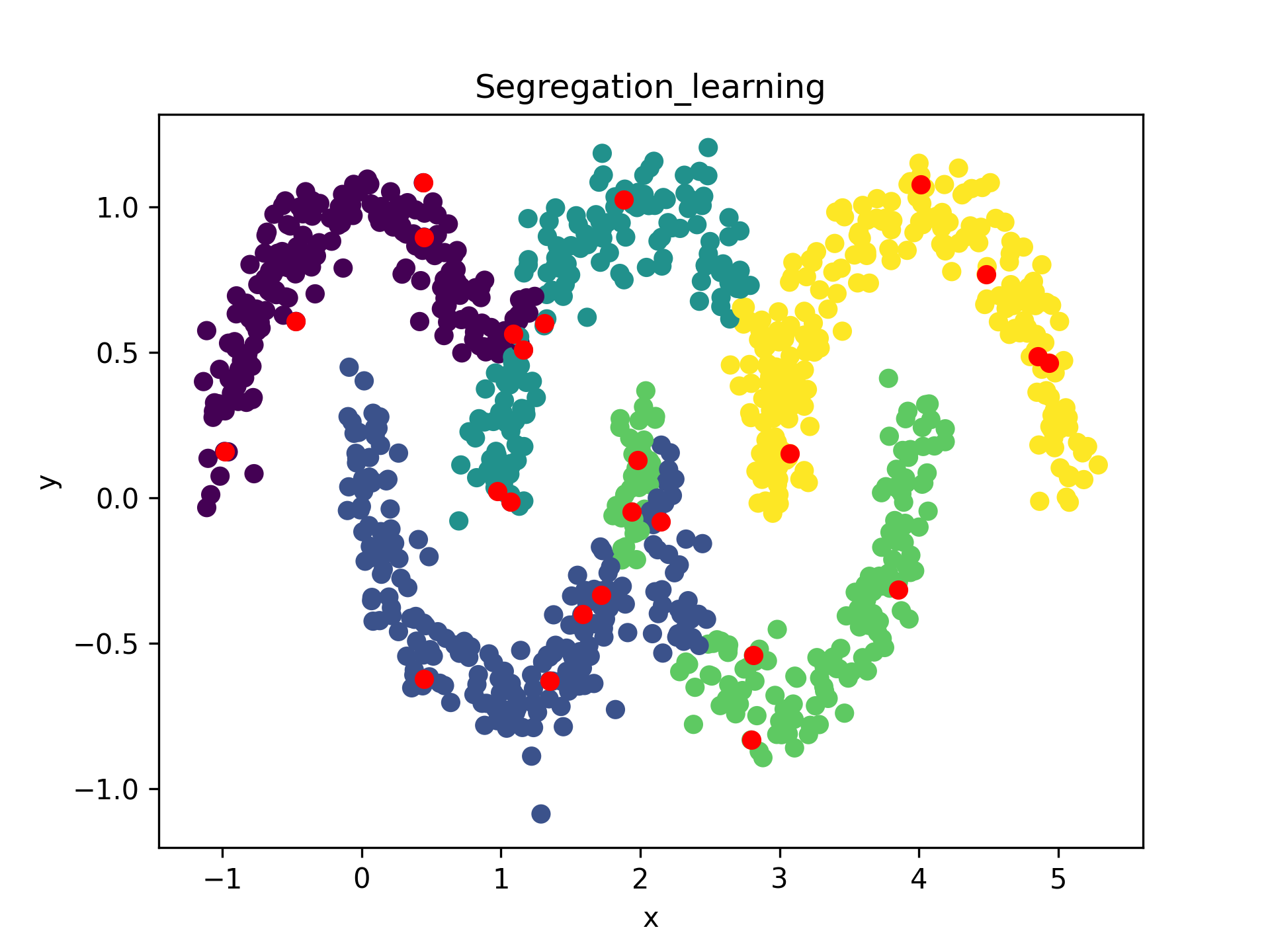
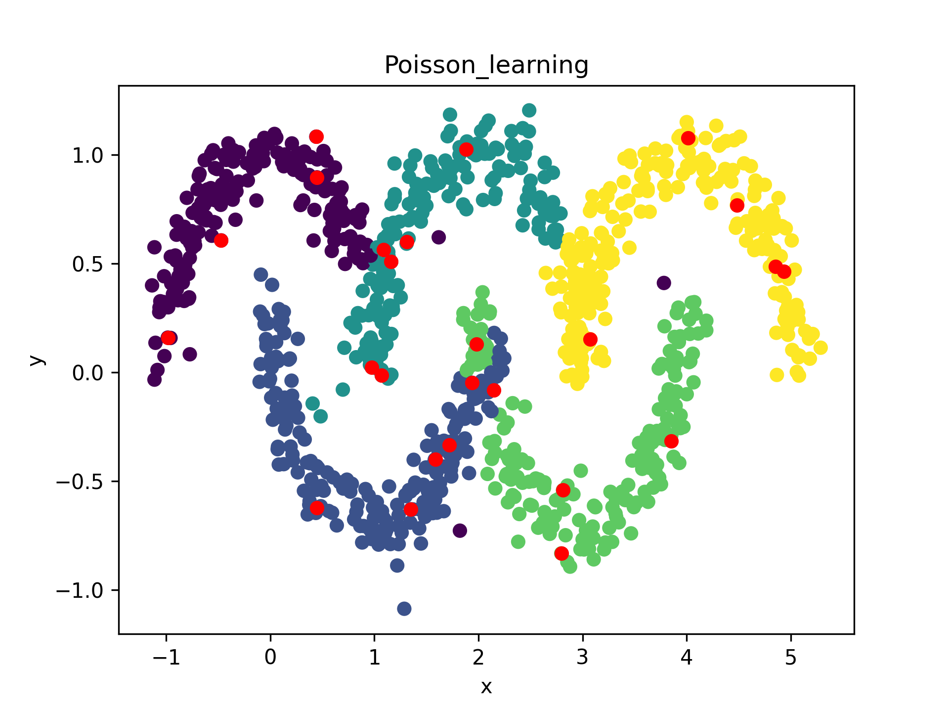
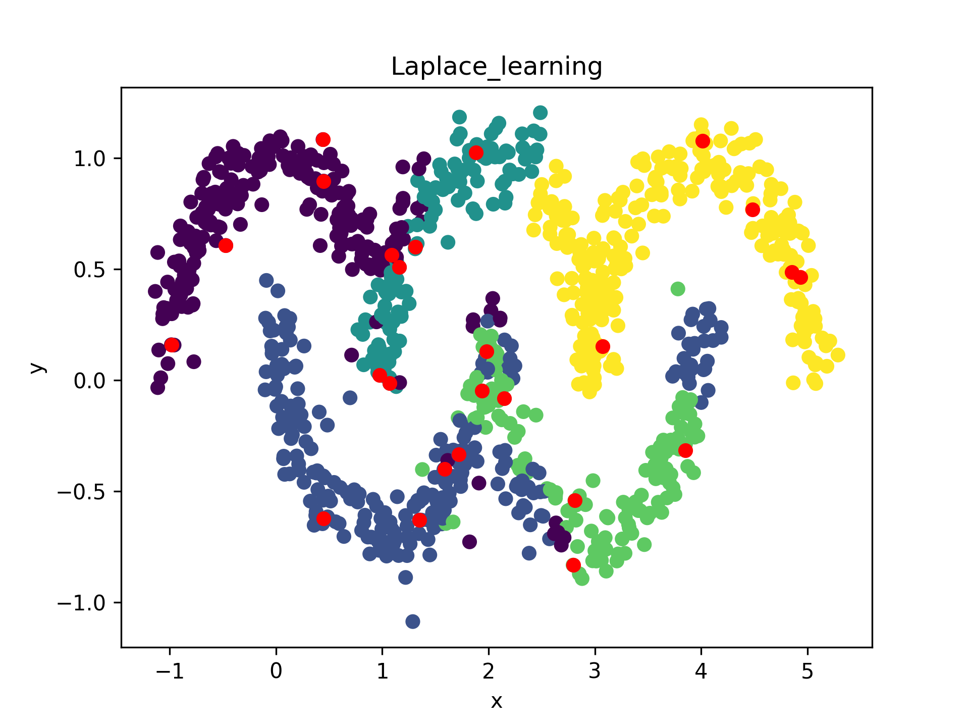
Figure 13. Comparison of Laplace, Poisson and Segregation learning algorithms for 5 classes and initial 5 labels per class.

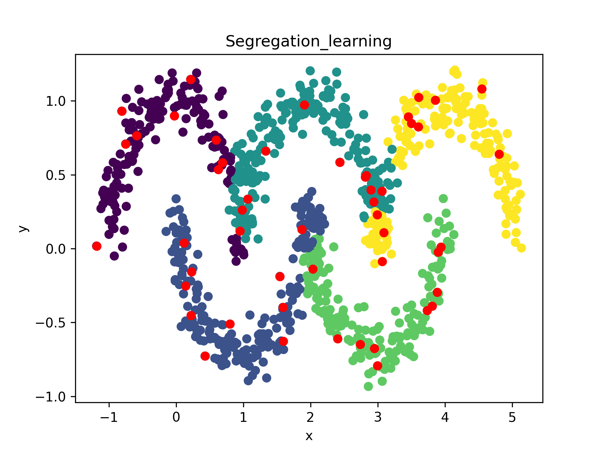
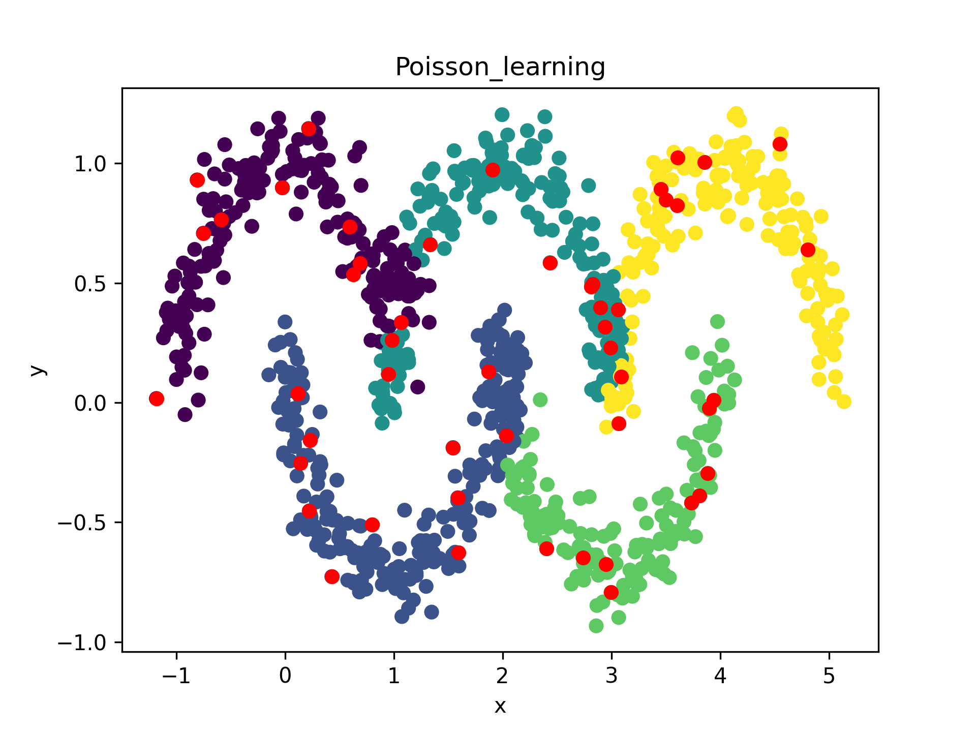
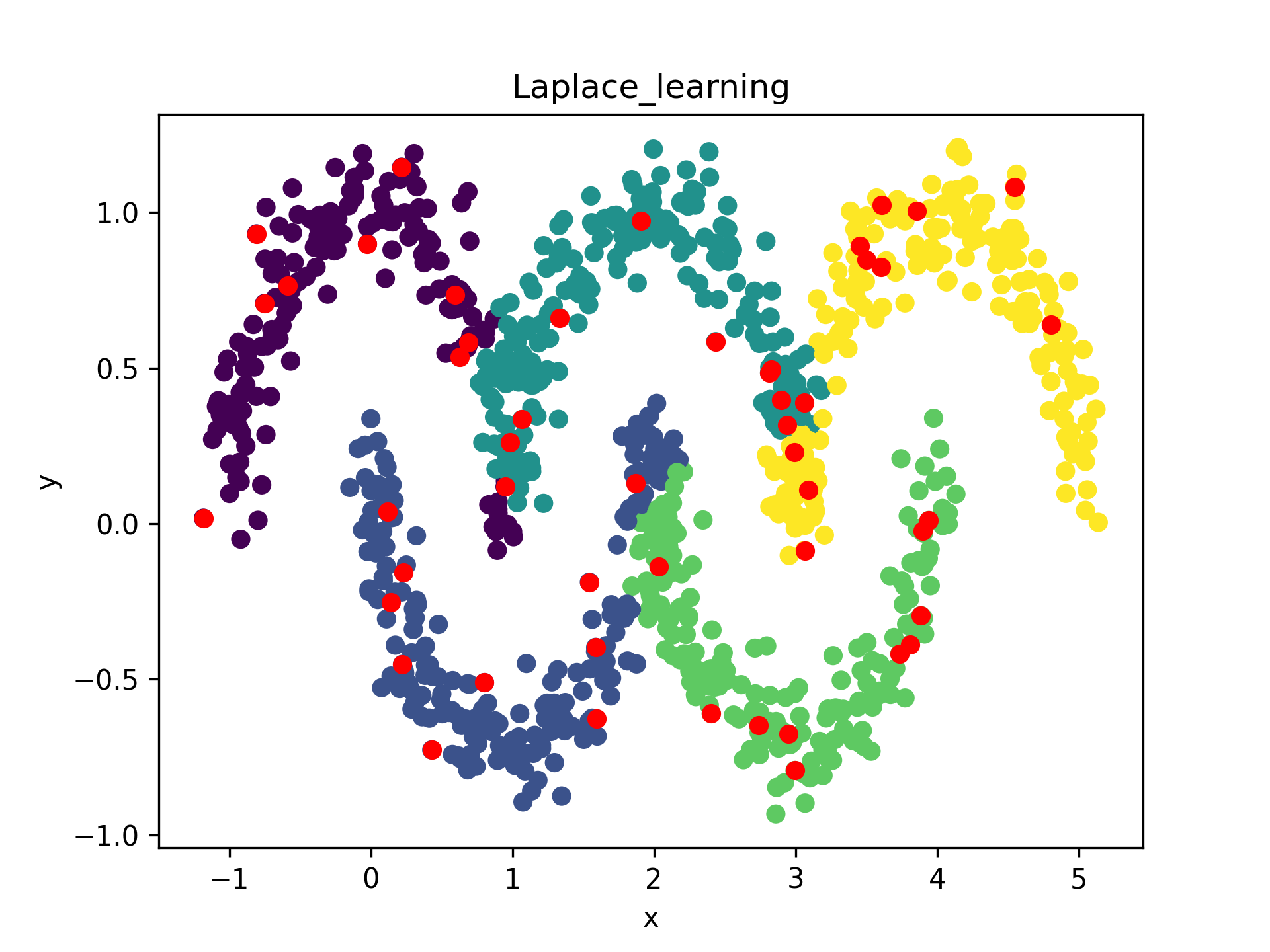
Figure 14. Comparison of Laplace, Poisson and Segregation learning algorithms for 5 classes and initial 10 labels per class.

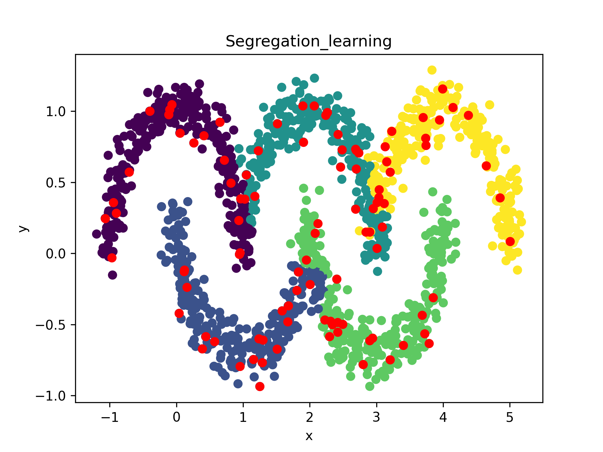
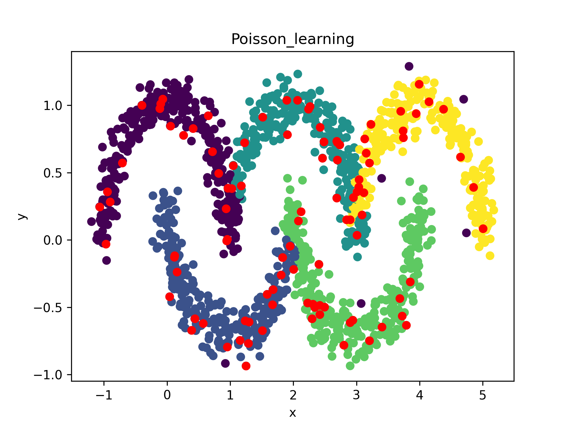
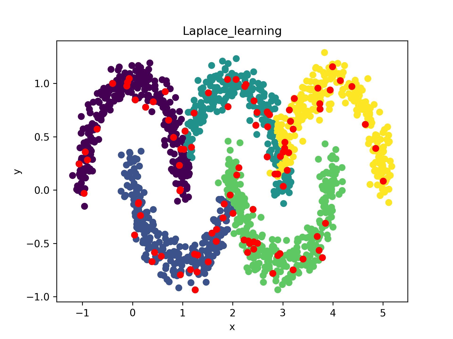
Figure 15. Comparison of Laplace, Poisson and Segregation learning algorithms for 5 classes and initial 20 labels per class.

Table 1. Average accuracy scores over 100 trials for 3 classes on MNIST dataset.

Labels per class	2	3	4	5	10
Laplace learning	31.3	45.4	58.2	67.7	83.4
Poisson learning	93.6	94.5	94.9	95.3	96.7
Segregation learning	90.3	92.1	93.5	95.4	96.2

Table 2. Average accuracy scores over 100 trials for 3 classes on MNIST dataset.

Labels per class	20	40	80	100	120
Laplace learning	88.6	91.3	93.7	95.2	97.6
Poisson learning	95.6	97.2	97.9	98.3	99.4
Segregation learning	94.3	96.7	98.2	98.8	99.2

7. Conclusion

In this work we develop several semi-supervised algorithms on graphs. Our main algorithm is a new approach for graph-based semi-supervised learning based on spatial segregation theory. The method is efficient and simple to implement. We presented numerical results showing that Segregation Learning performs more or less as Poisson Learning algorithm not only at high label rates, but also at low label rates on MNIST dataset.

8. Appendix

In this section, we record two important statements in graphs, Poincaré inequality and maximum principle for superharmonic functions.

Proposition 8.1 (Poincaré inequaity).

Assume the graph ${\mathcal{X}}$ is connected. For every $\Gamma\subset{\mathcal{X}}$, there exists constant $\lambda_{1}>0$, the first eigenvalue of Laplacian, such that

$$\lambda_{1}\|u\|_{\ell^{2}({\mathcal{X}})}\leq\|\nabla u\|_{\ell^{2}({\mathcal{X}}^{2})}$$

for all $u\in\ell^{2}({\mathcal{X}})$ satisfying $u=0$ on $\Gamma$.

Proof.

By the contradiction, we may assume that there exist the sequence $u_{n}$ such that

$$\|\nabla u_{n}\|_{\ell^{2}({\mathcal{X}}^{2})}\leq\frac{1}{n}\|u_{n}\|_{\ell^{2}({\mathcal{X}})},\quad u_{n}=0\text{ on }\Gamma.$$

Let $\hat{u}_{n}:=u_{n}/\|u_{n}\|$, then $\|\nabla\hat{u}_{n}\|\rightarrow 0$. The sequence $\{\hat{u}_{n}(x)\}_{n}$ is uniformly bounded ($|\hat{u}_{n}(x)|\leq\|\hat{u}_{n}\|=1$) and so there is a subsequence $\hat{u}_{n_{i}}$ and the limit function $u$ such that $\hat{u}_{n_{i}}(x)\rightarrow u(x)$ for every $x\in{\mathcal{X}}$. Hence, $\nabla\hat{u}_{n_{i}}\rightarrow\nabla u$, and so $\nabla u=0$ which yields that $u$ is a constant function on ${\mathcal{X}}$. On the other hand, from the boundary data $\hat{u}_{n_{i}}=0$ on $\Gamma$ we obtain that $u=0$ on $\Gamma$ and so $u=0$ on all of the graph. This contradicts the condition $\|u\|=\lim_{n_{i}\rightarrow\infty}\|\hat{u}_{n_{i}}\|=1$. ∎

Proposition 8.2 (Maximum principle).

Assume the graph ${\mathcal{X}}$ is connected. Let $p(x)$ be a nonnegative function on ${\mathcal{X}}$, and $u$ satisfies ${\mathcal{L}}u+p(x)u\geq 0$ in ${\mathcal{X}}\setminus\Gamma$. If $u\geq 0$ on $\Gamma$, then $u\geq 0$ in ${\mathcal{X}}$.

Proof.

Define $A^{+}:=\{x\in{\mathcal{X}}:u(x)\geq 0\}$ and $A^{-}:=\{x\in{\mathcal{X}}:u(x)<0\}$. Let $v:=\max(-u,0)$ and multiply by the equation to get

$$0\leq({\mathcal{L}}u+pu,v)= (\nabla u,\nabla v)_{\ell^{2}({\mathcal{X}}^{2})}+(pu,v)$$

$$= \frac{1}{2}\sum_{x,y\in{\mathcal{X}}}w_{xy}(u(x)-u(y))(v(x)-v(y))+\sum_{x\in{\mathcal{X}}}p(x)u(x)v(x)$$

$$= -\frac{1}{2}\sum_{x,y\in A^{-}}w_{xy}(u(x)-u(y))^{2}-\sum_{x\in A^{-},y\in A^{+}}w_{xy}(u(x)-u(y))u(x)$$

$$-\sum_{x\in A^{-}}p(x)(u(x))^{2}\leq 0$$

If $A^{-}\neq\emptyset$, we can find an edge between $A^{+}$ and $A^{-}$ due to the connectedness of $G$. (Note that the boundary condition ensures that $A^{+}\neq\emptyset$.) But the second term in the above calculation yields that $w_{xy}=0$ for every $x\in A^{-}$ and $y\in A^{+}$. Therefore, we must have $A^{-}=\emptyset$. ∎

REFERENCES

• [1] R. K. Ando, T. Zhang, Learning on graph with Laplacian regularization, In Advances in Neural Information Processing Systems, pp. 25โ€“32, 2007.
• [2] A. Arakelyan, R. Barkhudaryan, A numerical approach for a general class of the spatial segregation of reaction-diffusion systems arising in population dynamics. Computers and Mathematics with Applications 72, (2016), 2823-2838.
• [3] A. Arakelyan Convergence of the finite difference scheme for a general class of the spatial segregation of reactionโ€“diffusion systems. Computers and Mathematics with Applications, 75, (2018) 4232-4240.
• [4] A. Arakelyan, F. Bozorgnia, On the uniqueness of the limiting solution to a strongly competing system. Electronic Journal of Differential Equations, 96, (2017) 1-8.
• [5] M. Belkin, P. Niyogi, Using manifold structure for partially labelled classification. In Advances in Neural Information Processing Systems, 2002.
• [6] A. L. Bertozzi, A. Flenner, Diffuse interface models on graphs for classification of high dimensional data. Multiscale Modeling and Simulation, 10(3):1090โ€“1118, 2012.
• [7] F. Bozorgnia, A. Arakelyan, Numerical algorithms for a variational problem of the spatial segregation of reaction-diffusion systems. Applied Mathematics and Computation 219 (17), 8863-8875.
• [8] F. Bozorgnia, Numerical algorithms for the spatial segregation of competitive systems. SIAM J. Sci. Comput, 31, (2009) 3946-3958.
• [9] L. Caffarelli, F. Lin, Singularly perturbed elliptic systems and multi-valued harmonic functions with free boundaries. J. Amer. Math. Soc. 21, no. 3, (2008) 847โ€“862.
• [10] J. Calder, B. Cook, M. Thorpe, and D. Slepฤev. Poisson Learning: Graph based semi-supervised learning at very low label rates. Proceedings of the 37th International Conference on Machine Learning, PMLR, 119:1306โ€“1316, 2020.
• [11] J. Calder, The game theoretic p-Laplacian and semisupervised learning with few labels. Nonlinearity, 32 (1), 2018.
• [12] J. Calder, Consistency of Lipschitz learning with infinite unlabeled data and finite labeled data. SIAM Journal on Mathematics of Data Science, 1:780โ€“812, 2019.
• [13] J. Calder, J. and D. Slepฤev, Properly-Weighted graph Laplacian for semi-supervised learning. Applied mathematics and optimization, 82(3), 1111-1159, 2020.
• [14] M. Conti, S. Terracini, S., and G. Verzini, A variational problem for the spatial segregation of reaction-diffusion systems. Indiana University mathematics journal, 779-815, 2005.
• [15] X. Desquesnes, A. Elmoataz, O.Lezoray Eikonal equation adaptation on weighted graphs: fast geometric diffusion process for local and non-local image and data processing. Journal of Mathematical Imaging and Vision, Springer Verlag, 2013, 46 (2), pp.238-257. ff10.1007/s10851-012- 0380-9ff. ffhal-00932510f
• [16] A. El Alaoui, X. Cheng, A. Ramdas, M. J. Wainwright, and M. I. Jordan. Asymptotic behavior of lp-based Laplacian regularization in semi-supervised learning. In 29th Annual Conference on Learning Theory, pages 879โ€“906, 2016.
• [17] I. El Bouchairi, J. Fadili, A. Elmoataz, Continuum limit of $p$-Laplacian evolution problems on graphs: $L^{q}$ graphons and sparse graphs. https://arxiv.org/pdf/2010.08697.pdf.
• [18] H. Ennaji, Y. Quรฉau, A. Elmoataz, Tug-of-War games and PDEs on graphs: simple image and high dimensional data processing. 2022, https://hal.archives-ouvertes.fr/hal-03675971.
• [19] N. Garcรญa Trillos, M. Gerlach, M. Hein, and Slepฤev, Error Estimates for Spectral Convergence of the Graph Laplacian on Random Geometric Graphs Toward the Laplaceโ€“Beltrami Operator. In: Foundations of Computational Mathematics 20 ( 2020),pp. 827โ€“887. DOI: 10.1007/s10208-019-09436-w.
• [20] C. Garcia-Cardona, E. Merkurjev, A. L. Bertozzi, A. Flenner, and A. G. Percus, Multiclass data segmentation using diffuse interface methods on graphs, IEEE Trans. Pattern Anal. Mach. Intell. 36 (2014), 1600โ€“ 1613.
• [21] K. Ghasedi, X. Wang, C. Deng, and H. Huang, Balanced self-paced learning for generative adversarial clustering network. In Proceedings of the IEEE Conference on Computer Vision and Pattern Recognition, pp. 4391โ€“4400, 2019.
• [22] R. Kyng, A. Rao, S. Sachdeva, D. A. Spielman, Algorithms for Lipschitz learning on graphs. In Conference on Learning Theory, pp. 1190โ€“1223, 2015.
• [23] B. Nadler, N. Srebro, and X. Zhou, Semi-supervised learning with the graph Laplacian: The limit of infinite unlabelled data. Advances in Neural Information Processing Systems, 22:1330โ€“1338, 2009.
• [24] Slepฤev, D. and Thorpe, M., Analysis of p-Laplacian regularization in semisupervised learning, SIAM Journal on Mathematical Analysis, 51(3), pp.2085-2120, 2019.
• [25] Shi, Z., Osher, S. and Zhu, W., Weighted nonlocal laplacian on interpolation from sparse data. Journal of Scientific Computing, 73(2), pp.1164-1177, 2017.
• [26] Ulrike von Luxburg. A tutorial on spectral clustering. Statistics and computing, Vol. 17, 4 (2007),pp. 395โ€“416.
• [27] X. Zhu, Z. Ghahramani, and J. D. Lafferty, Semisupervised learning using Gaussian fields and harmonic functions. In Proceedings of the 20th International Conference on Machine learning (ICML-03), pp. 912โ€“919, 2003.