Causal identification for continuous-time stochastic processes
Abstract
Many real-world processes are trajectories that may be regarded as continuous-time “functional data”. Examples include patients’ biomarker concentrations, environmental pollutant levels, and prices of stocks.
Corresponding advances in data collection have yielded near continuous-time measurements, from e.g. physiological monitors, wearable digital devices, and environmental sensors. Statistical methodology for estimating the causal effect of a time-varying treatment, measured discretely in time, is well developed. But discrete-time methods like the g-formula, structural nested models, and marginal structural models do not generalize easily to continuous time, due to the entanglement of uncountably infinite variables. Moreover, researchers have shown that the choice of discretization time scale can seriously affect the quality of causal inferences about the effects of an intervention. In this paper, we establish causal identification results for continuous-time treatment-outcome relationships for general càdlàg stochastic processes under continuous-time confounding, through orthogonalization and weighting. We use three concrete running examples to demonstrate the plausibility of our identification assumptions, as well as their connections to the discrete-time g methods literature.
Keywords: observational studies, functional data, time-varying treatment, orthogonalization, weighting, g methods
1 Introduction
Many variables of interest are trajectories that can be considered as continuous-time stochastic processes taking values in finite, countable or uncountable state spaces. Longitudinal data have long been collected sparsely over time as proxies for continuous trajectories, e.g. the Framingham Heart Study [Mahmood et al., 2014], the Nurses’ Health Study [Colditz et al., 1997], and the Survey of Health, Ageing, and Retirement in Europe (SHARE) [Börsch-Supan et al., 2013]. Recent technology advances in data collection have yielded near continuous-time dense measurements, i.e. functional data. For example, heart rates from physiological monitors, physical activities from wearable trackers, PM2.5 levels from air quality sensors, stock prices from online trading platforms, and brain images from functional magnetic resonance imaging (fMRI) techniques. A wide variety of empirical studies have focused on the relationship between two trajectories. Examples include trajectories of close interpersonal contact on COVID-19 incidence [Crawford et al., 2022], climate changes on agriculture [Blanc and Schlenker, 2020], trajectories of low-density lipoprotein cholesterol levels on cardiovascular disease risks [Domanski et al., 2020], and socioeconomic status trajectories on cognitive functions [Lyu and Burr, 2016].
A central question in many scientific inquiries and policy evaluations is the causal effect of one trajectory (i.e. the treatment or intervention or exposure) on another trajectory (i.e. the outcome). Randomized experiments are often seen as the gold standard design for estimating unbiased causal effects. However, such experiments can be unethical, too difficult, or too expensive to implement in some scenarios. Instead, researchers often must resort to observational studies, where time-varying confounding and treatment-confounder (outcome) feedback can occur over time. Naïve adjustments for confounders in this setting can result in biased estimates of causal effects since the confounders may also be mediators of the effects of previous treatments on future outcomes [Hernán and Robins, 2020, Chap. 19, 20].
Most of the existing literature on causal inference for continuous trajectories has focused on the case of longitudinal data. For example, g methods [Hernán and Robins, 2020, Chap. 21], including the g-formula [Gill and Robins, 2001], marginal structural models and inverse probability-of-treatment weighting (IPTW) methods [Robins et al., 2000], and structural nested models and g-estimation methods [Robins, 1989], work with longitudinal data where each subject is measured at the same time points (i.e. regular longitudinal data). These methods can identify the causal effects of a sequence of treatments under assumptions such as sequential exchangeability, sequential consistency, and sequential positivity. These methods have been widely applied in empirical research in public health [e.g. Thompson et al., 2021, Vangen-Lønne et al., 2018, Vock et al., 2017, Saul et al., 2019].
However, when the data generating process (DGP) is continuous in time, issues arise for g-methods with discretely measured longitudinal data. For example, as Sun and Crawford [2022] point out, the discrete-time potential outcome notation has implicitly assumed no multiple versions of treatment or treatment variation irrelevance [VanderWeele, 2009], but this is rarely true: many continuous-time trajectories might coincide with a single observed sequence of discretely sampled treatments. These multiple distinct trajectories passing through the observe data comprise different versions of treatment, rendering some potential outcome notation ill-defined. In addition, the treatment assignment might depend on the unobserved values of the past treatment and covariate processes, causing violations of unconfoundedness.
Several causal estimands and identification strategies for continuous-time treatments and outcomes have been proposed. Most prior literature focuses on piecewise-constant treatment processes, e.g. time-to-event treatments, counting process treatments, and (marked) point process treatments. Among them, Yang [2021], Zhang et al. [2011], and Lok [2008] generalize g-estimation; Røysland et al. [2022], Hu et al. [2021], Saarela and Liu [2016], Røysland et al. [2011], and Johnson and Tsiatis [2005] generalize IPTW methods; and Rytgaard et al. [2022] generalize the g-formula.
However, many exposures in empirical studies change continuously and take values in an uncountable set, e.g. air pollutant concentrations and blood pressures. In this paper, we develop novel causal identification strategies for general càdlàg trajectories of treatments, covariates, and outcomes under the potential outcome framework. Examples include discrete-time DGPs, piecewise-constant processes, continuous processes (e.g. diffusions), and continuous processes with jumps (e.g. diffusions with jumps). Therefore, the proposed strategies provide a unifying solution to a large class of continuous-time causal questions.
In the following, we define causal estimands based on continuous-time potential outcomes, propose causal identification assumptions that generalize those employed in discrete-time g-methods, and present identification strategies mainly based on a continuous-time unconfoundedness condition. Our approach identifies causal parameters based on moment conditions. It takes the form of orthogonalization to remove measured confounding. Implicitly, it is also a weighting strategy by using the inverse of the “rate of change of the treatment” as weights. Three concrete causal DGPs satisfying all the identification assumptions are used as running examples for the exposition of the proposed strategies. Recently, Ying [2022] generalized the g-formula and IPTW to the continuous-time general stochastic treatment regimes setting. In contrast, our approach focuses on causal estimands corresponding to deterministic treatment regimes.
1.1 Setting and notation
Define a complete probability space , where is the sample space, is a -algebra, and is a probability measure. We consider a finite study period which ends at time , and define the index set . In the following, each -dimensional Euclidean space (or its subspace ) is equipped with its Borel -algebra (resp. ) [Jacod and Shiryaev, 2013, Kallenberg, 1997].
A process is càdlàg if all of its paths are right-continuous and admit left-hand limits. For a process admitting a left-hand limit at all , define its left-limit process as . Define the following càdlàg processes: the treatment process , the outcome process , and the covariate process . By convention, we use superscripts from to to represent each component of a multivariate process. Further denote . Denote as the treatment trajectory up to time , where (or , whichever is convenient) is the value of the observable treatment trajectory at time for . Similarly we define . In the following, we will omit when it is unambiguous.
The càdlàg potential outcome trajectory for a subject up to time is defined as
where represents the values of the outcome and covariates of a subject, had this subject precisely followed the predetermined static treatment trajectory of interest . We assume that a trajectory can only depend on the past, i.e., for . In the following, we also use or to denote .
The causal estimand of interest is the counterfactual average outcome evaluated at time , , under a deterministic treatment plan specified up to . This estimand can be used to compute the average treatment effect (ATE) of a treatment plan compared to a baseline treatment plan that is constant , i.e.
or a weighted average of counterfactual means, i.e.
where is a known distribution over the space of treatment plans under a stochastic intervention.
1.2 Informal motivation
We first provide an informal explanation of the main identification results. We will start from the traditional discrete-time setting. Without loss of generality, suppose the values of all relevant processes are observed at equidistant time points, i.e. with . Following the convention in Jacod and Shiryaev [2013], we use a prime notation to distinguish discrete-time and continuous-time processes. The observable data is at time , , where . For a deterministic static treatment plan , the corresponding potential outcome of interest is denoted as . It is the value of the outcome at the end of the study had the individual followed the treatment plan before the th time point. Let . Define the discrete-time filtration . Let be the baseline treatment plan with . The causal estimand is the counterfactual mean .
We further suppose that this DGP satisfies the following conditions which discrete-time g methods usually assume for causal identification [Hernán and Robins, 2020].
Assumption 2′ (Discrete-Time Sequential Exchangeability (DTSE)).
With observable data ,
. 111This version is called “conditional mean independence”, which is less restrictive than the “conditional independence” version .
Assumption 3′ (Discrete-Time Sequential Consistency (DTSC)).
For a treatment plan ,
Assumption 4′ (Discrete-Time Causal Structural Model (DTCSM)).
The potential outcome satisfies the following marginal structural model
where is a general function and . The structural model in Assumption 4′ is intended to simplify the exposition, and more complex structural models can also be compatible with the approach described in this paper.
Denote the true value of the parameter in the structural model as . By Assumptions 3′ and 4′,
Thus, to identify the average potential outcome, it suffices to identify the causal parameter . Consider the following function of :
| (1) |
We claim that solving the equation identifies . This is because
| (By Assumptions 3′ and 4′, ) | |||
The above identification strategy follows the idea of orthogonalization, by partialling out the effect of the observed past history (i.e. ) on the current treatment assignment . Then, by unconfoundedness (Assumption 2′), the remainder will be “orthogonal” to any functions . In the case above, . The orthogonalization idea has appeared in recent causal inference literature. For example, Chernozhukov et al. [2018] give a concrete example of using orthogonalization to estimate treatment effects with cross-sectional data in the presence of high-dimensional confounders. Bates et al. [2022] propose an orthogonalization form of parametric g-formula for discrete-time longitudinal data by partialling out the effect of the past history on the current covariates .
Next, we move towards the continuous-time setting. Define the differences and . Then, Equation (1) can be rewritten as
Note that the study period is and fixed. Thus, when tends to infinity, in analogy to how Riemann sums approach Riemann integrals, informally, the above sum will approach an Itô stochastic integral in continuous-time
which equals zero when evaluated at . As will be seen later, the stochastic process is the compensator of the treatment with respect to the observable history. Then, the process is the remainder of the treatment process after partialling out all the past observable information. This simple example demonstrates the main ideas behind our identification strategies in Sections 4 and 5.1. Its relation to weighting is explained in Section 5.2.
1.3 More setting and notation
We introduce more concepts and notations for continuous-time processes that will be needed to develop the proposed identification theory.
It is convenient to use a filtration to represent all the available information from the processes up to a given time. For a process taking values in a measurable space , define its natural filtration as , where . A complete filtration is sometimes needed for theoretical developments, but a natural filtration is not necessarily complete. Thus, we define its completion. Let be the set of all -zero-measure sets in . For a filtration , define its completion as the filtration with , which is the smallest complete filtration such that . Here, is the smallest sigma-field generated by and , i.e. , where .
Define with . Thus, represents all the information available from the observable data up to time . Let be the -field generated by the potential outcome trajectory. It contains all the information of the potential outcome under the treatment plan within the study period . Define the initially enlarged filtration , where
and is the potential outcome trajectory when the treatment of interest is the constant function on , i.e. for all . Intuitively, if one has access to , then one not only knows the trajectories of and the potential outcome up to time , but can also peek into future values of the potential outcome up to the end of the study. Therefore, we call the factual (or observable) filtration, and the counterfactual filtration.
Data in statistics can often be described as the sum of signal and noise. This idea is captured by the notion of a special semimartingale [Kallenberg, 1997] for stochastic processes. We focus on the case where the treatment process is an -special semimartingale. Formally, given a generic filtration , a real-valued process is called an -semimartingale if
where , is -measurable, is an -local martingale, and is a càdlàg -adapted finite variation process. Furthermore, a semimartingale is an -special semimartingale if is also -predictable. Then the decomposition is unique (i.e. the canonical decomposition), and is called the compensator of .
Intuitively, reflects the infinitesimal systematic change of the treatment process given the past history, while reflects the remaining variation (i.e., the “random noise”). An -valued process is a (special-) semimartingale if each of its components is a (special-) semimartingale. Examples of special semimartingales include submartingales or supermartingales, counting processes, and continuous semimartingales (e.g. diffusions and Itô processes). We focus on special semimartingales for two reasons: (1) we can resort to the powerful results from Itô calculus, since the semimartingales form the largest class of processes as integrators for which the Itô integral can be defined; and (2) the uniqueness of the decomposition of special semimartingales avoids unnecessary technicalities for practical applications.
For convenience, we summarize our setting:
Assumption 1 (Setting).
We assume
(1) Processes , the static treatment plan , and the potential outcome process are càdlàg .
(2) is an -special semimartingale.
2 Examples
We present three classes of continuous-time DGPs as running examples. We will verify our identification assumptions for each of them later, showing that the statistical model is nontrivial. Figure 1 shows realizations from each example DGP.
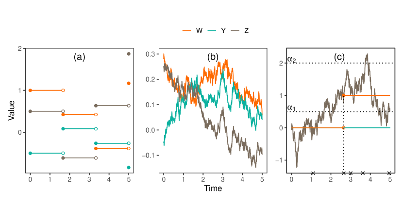
2.1 Example 1: Discrete-time DGPs
This is the example described in Section 1.2, where the true DGP is discrete-time. Any discrete-time DGP has a unique corresponding continuous-time representation [Jacod and Shiryaev, 2013, Chap. 1] as step functions, and thus the discrete-time DGP is a special case of our general setting. Recall that the causal estimand is , the discrete-time filtration is , and with . We will focus on its equivalent continuous-time representation below. A realization of under this DGP is shown in Figure 1(a).
Define the continuous-time processes , which are step functions of . Here is the largest integer that is not greater than the real number . Define with . is the history of all the observed information up to each time . Define with . The -algebra will remain the same between two observation time points since no new information is observed in between. By Jacod and Shiryaev [2013, Chap. 1.4], since is -adapted, is an -semimartingale. Then, given , will be an -special semimartingale. Thus, Assumption 1 is satisfied.
2.2 Example 2: Continuously-valued treatment and outcome
Many variables in observational studies are continuous, e.g. blood pressures and household incomes. We show an example where are continuous random variables. We use the multivariate Ornstein-Uhlenbeck process [Iacus, 2009, Chap. 1], a type of diffusion processes, as the DGP. It has wide applications in physics [Uhlenbeck and Ornstein, 1930], evolutionary biology [Hunt, 2007], and mathematical finance [Leung and Li, 2015, Björk, 2009].
Let be a -dimensional standard Brownian motion with respect to its natural filtration. Define as the outcome process, the treatment process, and the covariate process, with initial random vector which is independent of . Define where . We consider a 3-dimensional OU process [Gardiner et al., 1985] as the causal mechanism, which is the unique -strong solution of the following SDE:
| (2) |
where
are constant matrices. Intuitively, the drift parameter describes the instantaneous expected influence between observable processes, while the diffusion parameter specifies the structure and magnitudes of the impact of the external noises on observable processes. For example, the parameter in Equation (2) indicates that the exposure and outcome processes do not have common external sources of influence. This specification has important implications with regard to the unconfoundedness condition, as will be shown later. A realization of under this DGP is shown in Figure 1(b).
Given an arbitrary treatment trajectory of interest , the potential outcome process is the strong solution of
| (3) | ||||
with . Suppose are all observable, while are unmeasured, then we have observable filtration with . The enlarged filtration is . Since is a diffusion process, it is an -special semimartingale, and therefore Assumption 1 is satisfied.
2.3 Example 3: Time-to-event treatment and outcome
Time-to-event variables are common in public health and social sciences, e.g. disease occurrences and financial defaults. In the following, we describe a causal DGP where both the treatment and outcome are time-to-event data and the covariate is a continuous process. For example, the treatment is the time-to-initiation of a medical treatment, and the outcome is the time to an adverse health event.
Let and be a standard Poisson process and a standard Brownian motion respectively, with respect to their natural filtrations. Define as the outcome, treatment and covariate processes with , which are all observable. Define the random time at which first rises above a threshold as , and the time at which rises above another threshold as , and by convention let . Define the corresponding indicator processes and . Define with . The causal DGP is the -strong solution of the following SDE:
Here, are model parameters, where . As an interpretation of the above DGP, represents the severity of a disease whose volatility of progression is characterized by , and when passes a certain threshold (i.e. ) at time , the subject will start to seek medical treatment and wait for a random time before the procedure/surgery or medication become available. If the disease progresses to at time before the medical treatment starts, then the subject will experience a severe adverse event. Since is a counting process, Assumption 1 is obviously satisfied. A realization of is shown in Figure 1(c).
For a one-jump treatment plan , the potential outcome process is
where and . We thus define the observable filtration with , and the expanded filtration with .
3 Definition of identification
Before describing our identification strategies, we need to first define the meaning of “identification” in this paper. Following Lewbel [2019], Basse and Bojinov [2020], we now formalize what identification entails generally. Define the statistical model as , which contains all the DGPs that satisfy the specified assumptions. For a DGP , a function defines the estimand of interest. Define as the set of possible estimand values. Define function mapping the DGP to observable information, and as the image of . Denote the true DGP as , and . Thus is what we can observe from the data.
Definition 1.
An identification strategy is a function such that
In other words, is an identification strategy if and only if ’s set of zeros is a superset of the image of under the function , , i.e.
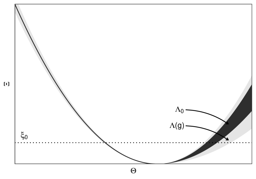
We call an identification strategy sharp if . We say that point-identifies when if and only if ; otherwise, we say partially identifies .
For example, for a metric space , when there is an explicit function such that , the corresponding identification strategy is sharp and point-identifies . Figure 2 is a visual representation of the above concepts. In panel (b), the black area in is , and the grey area is . Since is a strict superset of , is not sharp; since a single value of may correspond to many different ’s such that , partially identifies .
The causal identification is a special case of the above definition where the estimand is a causal estimand that is related to counterfactual variables. In particular, in our causal question, different DGP ’s correspond to different functions mapping from , where is the set of all treatment plans. We omit the notation showing this dependence on when it is not ambiguous. Then, the causal estimand is and the observable information is . Knowing the function implies the usual saying that “an infinite number of i.i.d. realizations of are available”. In Section 4, we will introduce the assumptions that specify the statistical model , and in Section 5, we will give a class of identification strategies .
4 Identification assumptions
In this section, we introduce causal identification assumptions that place restrictions on the statistical model for the causal DGP of continuous-time processes. Broadly, the assumptions generalize standard assumptions from the discrete-time g-methods literature: sequential exchangeability, sequential consistency, sequential positivity, and structural models [Hernán and Robins, 2020].
4.1 No Information Drift (NID)
In observational studies, when there is unmeasured confounding, the assignment of treatment at time depends not only on the observable information before time , i.e. , but may also depend on information about the potential outcome in the future (e.g. ). For causal identification, we need a “no unmeasured confounding”-type condition. The following condition is a continuous-time generalization of the “sequential exchangeability” condition in the discrete-time g methods literature [Hernán and Robins, 2020, Chap. 19]. Recall that the -canonical decomposition of is , where is the local martingale part, and is the compensator.
Assumption 2 (No Information Drift (NID)).
The canonical decompositions of the treatment process with respect to and are the same.
Assumption 2 indicates an invariance under a change of filtration. It is equivalent to the statement that is both an - and a -local martingale, since if is an -predictable finite variation process, it is also a predictable finite variation process with respect to .
Information drift is a well-known concept in the stochastic analysis literature [Ankirchner et al., 2006]. Generally, under an enlargement of filtration, may not be a -local martingale, or even a -semimartingale. When is a real-valued continuous semimartingale and is a -semimartingale, Ankirchner et al. [2006] shows that
where is a -local martingale, is the quadratic variation process of , and is a unique (up to indistinguishability) -predictable process. The integrand is often called the information drift of the expansion from to . It reflects how the additional information contained in but not in changes the systematic behavior of . In our setting, reflects how the asymmetric information related to the potential outcome that treatment decision-makers use (consciously or unconsciously) but the observational data does not include, will influence the assignment mechanism of treatment. This translates the concept of unmeasured confounding to the concept of asymmetric information. Assumption 2 implies that
which means no information drift and implies no unmeasured confounding.
When is a time-to-event treatment, e.g. treatment initiation or termination, and the treatment process is defined as , the No Unmeasured Confounding conditions in existing continuous-time causal inference literature (e.g. Zhang et al. [2011], Hu and Hogan [2019], Yang [2021]) are special cases of Assumption 2, using decompositions of random times.
Based on Assumption 2, we formally propose a definition of “confounders” for trajectories below, in the sense that these covariates form a “sufficient adjustment set” rendering NID satisfied.
Definition 2.
For the treatment process , and the outcome process , a set of covariate processes is called confounders, if the canonical decompositions of under the filtration and the filtration are the same.
Next, we verify Assumption 2 for Example 1-3. These concrete examples show the connections to the discrete-time setting, and provide insights into continuous-time confounding. We will show that discrete-time sequential exchangeability (Assumption 2′) is a special case of no information drift (Assumption 2). However, no information drift does not imply discrete-time sequential exchangeability unless is both an - and -martingale instead of a local martingale. Similarly, we verify that there is no information drift in DGPs in Examples 2 and 3. We formally state the results in Proposition 1, 2, and 3. Proofs are presented in Appendix A.
Proposition 1 (NID for Example 1).
Proposition 2 (NID for Example 2).
Using notations in Section 2.2, the canonical decompositions of with respect to and are the same.
Proposition 3 (NID for Example 3).
Using notations in Section 2.3, the canonical decompositions of with respect to and are the same.
4.2 Continuous-Time Consistency Assumption (CTC)
Generalizing discrete-time sequential consistency assumption[Hernán and Robins, 2020, Chap. 19], we make the following assumption for the continuous-time case to link the potential outcomes to observable outcomes.
Assumption 3 (Continuous-Time Consistency (CTC)).
For all treatment trajectories , if for , then we observe and . Furthermore, and .
Assumption 3 requires that there is no interference between individuals, and there are no multiple versions of the treatment. Examples 1-3 clearly satisfy this assumption.
4.3 Causal Structural Model (CSM)
For a treatment plan , define as the individual treatment effect of at time . By Assumption 3, we have . We make the following causal structural assumption on , which depicts the relationship between a specified intervention and the potential outcome. Note that the baseline potential outcome process is left unrestricted.
Assumption 4 (Causal Structural Model (CSM)).
The treatment effect is -adapted and is known up to the causal parameter , i.e. .
For example, the treatment effect might be represented by a function of the cumulative treatment delivered, e.g. , where the unknown function describes how the the effects of prior treatments accrue. Another example for a counting process outcome is , where the counting process is adapted to and is known from the observable data. Note that can be different among subjects, and can have finite dimensions (e.g. Euclidean spaces) or infinite dimensions (e.g. function spaces).
Suppose that the filtration records all the relevant information for the causal system and thus . Then in general, is -adapted, but not necessarily -adapted. However, in many cases, Assumption 4 may be satisfied. For example, the unobserved information may cancel out when we subtract from . We verify Assumption 4 for Examples 1-3.
Example 1 (Continued)
By Assumption 4′, , and . Then the corresponding continuous-time representation of the treatment effect becomes
| (4) |
which is deterministic and thus adapted to , and parameterized by a 1-dimensional .
Example 2 (Continued)
Example 3 (Continued)
Since is not influenced by , we have . Then it is easy to see that
| (6) |
Since is knowable from observable data and is -adapted, then is -adapted, and is parameterized by .
4.4 Continuous-Time Positivity (CTP)
In discrete time, the sequential positivity condition[Hernán and Robins, 2020, Chap. 19] is needed so that sufficient randomness exists in the treatment assignment at each time point after conditioning on the past. As mentioned above, is the “noisy” component of the treatment. Thus, we extend the sequential positivity condition to the continuous-time setting by imposing the following condition on .
Assumption 5 (Continuous-Time Positivity A (CTP-A)).
The local martingale is not constant zero.
Assumption 5 is equivalent to requiring that or is not an -predictable finite variation process. This assumption will be violated, for example, if has continuously differentiable sample paths. In real-life applications, inevitable noises in the treatment assignment often render the sample paths “rough” and thus ensure the satisfaction of Assumption 5. Examples 1-3 clearly satisfy this assumption because the treatments are not -predictable finite variation processes.
5 Identification results
We will first present our main identification strategies through orthogonalization, and then explain the connection to the weighting approach.
5.1 Main identification strategy
Suppose the statistical model satisfies Assumptions 1 to 5, and the true causal DGP is in . Recall that the probability space is fixed, and that the measurable functions depend on the DGP , where we omit the explicit notation of this dependence for conciseness. Our observable information is , and our estimand of interest is . We will develop a moment-based identification strategy such that . In fact, to identify , we only need to identify , the true causal parameters in under .
Recall that is the -dimensional local martingale part of the -canonical decomposition of , and define to be the quadratic covariation process of two generic processes . Define for an integer . Define the -dimensional process with
| (7) |
and ’s are Borel-measurable functions from to that can be arbitrarily chosen. The following theorem establishes a wide range of identification strategies.
Theorem 1 (Main).
Under Assumptions 1 to 5, suppose
(a) can be explicitly calculated with respect to .
(b) .
Define an -valued function
where the integral is in the Itô sense with respect to the filtration . Arrange elements of into a -column vector, denoted as . Let be an arbitrary positive-definite weighting matrix. Then
| (8) |
is an identification strategy for for all in the sense of Definition 1. Equivalently,
| (9) |
identifies .
Remark 1.
can be any continuous functions from to . For example,
using polynomials. It may often be helpful to incorporate covariate information in the moment conditions to increase efficiency, e.g. , where is an arbitrary component of the covariate process.
Remark 2.
Intuitively, our identification strategy is based on a stochastic integral under filtration . When , the integrand of the integral is a -predictable process that depends on the value of the potential outcome in the future, which is by definition adapted to . The integrator is both an - and -local martingale. Therefore, we can use it as an integrator when it is considered as a -local martingale, and identify it from observable data when it is considered as an -local martingale. Then, under weak regularity conditions, the -stochastic integral is a zero-mean martingale.
Proof of Theorem 1.
Without loss of generality, we will prove that is a solution to
| (10) |
for all in . It follows the same argument to prove for .
(1) We will first show that is a -predictable process.
By Assumption 3 and 4, . Define to be the -predictable -algebra on , which is generated by all continuous -adapted processes. Then, obviously the constant process is a -predictable process. Since by Assumption 1, are -adapted càdlàg processes, then their left-limit processes are left-continuous (i.e. càg) processes, and thus are -predictable processes. The deterministic function is clearly also -predictable. Thus, since each is a Borel-measurable function, then is also -measurable, and therefore is a -predictable process.
(2) We then show that with respect to filtration is a zero-mean martingale under .
By Assumption 1, 2, and 5, is a nontrivial - and -local martingale with , and it can be explicitly identified from observable data. Taking as the integrand and as the integrator, since , by Itô Isometry, the resulting stochastic integral is an -bounded -martingale starting from zero. Thus, we have proved Equation (9), and it can be easily extended to Equation (8). ∎
By the uniqueness of canonical decompositions, there is a function mapping to its compensator , which establishes the existence of a nonparametric point-identification strategy for . Thus, our identification is nonparametric in nature, since can also be infinite-dimensional. We additionally require that can be explicitly calculated. This is the case for any discrete-time adapted processes embedded in continuous time by definition (thus including Example 1), many counting processes [Aven, 1985], many processes specified by stochastic differential equations, and special semimartingales that satisfy certain regularity conditions, e.g. Knight [1991].
We show below applications of Theorem 1 to Examples 1 and 3. See Section 6 for a detailed application of Theorem 1 to estimate causal parameters in Example 2.
Example 1 (Continued)
By Equation (4) and Assumption 3,
In the discrete-time representation, the -compensator of can be explicitly written as , whose continuous-time representation is the -compensator of . Since we have verified that the DGP in Example 1 satisfies Assumption 1 to 5, thus we can apply Theorem 1 with an arbitrary function in and a weighting matrix . We choose
and . Note that and dim. Thus we use the fact that and get a valid identification strategy
Since the integrator is a step function, after simplification we have the discrete-time representation as
The above function from the continuous-time strategy coincides with Equation (1) in essence, which is derived under a discrete-time strategy.
Example 3 (Continued)
By Equation (6) and Assumption 3,
where is the causal parameter. In the proof of Proposition 3, we have shown that the -local martingale part of is
where is a nuisance parameter. By choosing
Theorem 1 gives
Solving the above equations will identify causal parameters . Equivalently, if we define to be the jump time of , which is observable, and let if never jumps in , and define , the above equations can be simplified as
5.2 An inverse weighting aspect of Theorem 1
Weighting methods are widely used in causal inference, e.g., Inverse Probability-of-Treatment Weighting (IPTW) in conjunction with marginal structural models [Robins et al., 2000], and balancing weights [Ben-Michael et al., 2021]. We show that after straightforward manipulations of the integrator in Theorem 1, we will have a weighting strategy. Intuitively, by using the Inverse Rate of change of the Treatment ’s -predictable part as weights (IRTW), we create a pseudo-population where subjects with different treatments are “exchangeable”.
We first state a new “Positivity”-type assumption below. Special cases of it considering counting process treatments have appeared in existing continuous-time IPTW literature, e.g. Hu et al. [2021]. This alternative “Positivity” assumption will replace Assumption 5 in the weighting identification strategy. Recall that .
Assumption 6 (Continuous-Time Positivity B (CTP-B)).
The -compensator of admits the form , where is an -predictable process, and .
CTP-B implies that we can find a well-behaved rate of change function of . For instance, the intensity process of a counting process treatment could be positive for all . One concrete example is that
where is a deterministic baseline function that is positive for all , and is a standard Poisson driving process. Then, . Note that CTP-B can be more restrictive than its alternative CTP-A (Assumption 5). However, when it is satisfied, it allows an alternative identification strategy.
We formally state our weighting strategy in Corollary 1 below, where is used as weights. Define as in Equation (7). Define and is a real-valued Borel-measurable function which can be arbitrarily chosen. For a generic jointly measurable process , define its -predictable projection as , which is the unique -predictable process such that for all -predictable times .
Corollary 1 (Weighting).
Under Assumptions 1, 2, 3, 4, and 6, suppose that for all ,
(a) can be explicitly calculated,
(b) ,
(c) is locally integrable.
Define an -valued function
| (11) |
where the integral is in the Itô sense with respect to the filtration . Arrange elements of into a -column vector, denoted as . Let be an arbitrary positive-definite weighting matrix. Then
is an identification strategy for for all in the sense of Definition 1. Equivalently,
identifies .
Remark 3.
In the simplest case, by setting , . More complex ’s may increase efficiency in estimations.
Intuitively, may not be zero due to the correlation between the treatment increments and the centered potential outcomes . This correlation is removed by reweighting with the “propensity of treatment” . See Appendix A for the formal proof.
6 Simulation study
To provide a concrete application of the main identification strategy in Theorem 1, we demonstrate how to estimate counterfactual means from data generated by the DGP in Example 2. The treatment plan of interest is , denoted as , and the estimand is . Note that we focus on the identification in this paper, and thus implement a working estimation procedure below. We will study the theoretical properties of the estimators in future work.
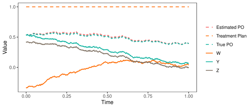
We generate full trajectories222Numerically, we use the Euler scheme [Iacus, 2009] to simulate trajectoriesaccording to Equation (2) on with
where MVN is the multivariate normal distribution. A realization is shown in Figure 3. By Equation (5), we correctly specify the individual treatment effect as
where the causal parameter is a function of , and the true value . Since , we need to specify at least 4 estimating equations. Define
To apply Theorem 1, we need to explicitly compute . Thus, we define the following correctly specified nuisance model
where is the nuisance parameter whose true value is , and is a standard Brownian motion. Denote , and let be a time grid on with . Then can be easily estimated by solving the following estimating equations:
| (12) |
, where is the empirical measure. Denote the estimate from Equation (12) as , then can be explicitly estimated as
By Equation (8) and choosing to be the identity matrix, we minimize the sample criteria function
| (13) |
and define our estimator .
7 Discussion
In this paper, we propose novel causal identification strategies for general continuous-time càdlàg processes under time-varying treatments and treatment-confounder feedbacks, which has been inspected from two perspectives: orthogonalization and weighting. We focus on the special semimartingale treatments, which include the rarely studied but widely seen case of continuously valued treatments.
The proposed strategies rely on an “unconfoundedness”-type assumption, the No Information Drift assumption (Assumption 2). This key assumption indicates an invariance under a change of filtration (the factual filtration versus the counterfactual filtration ). It has an intuitive interpretation that the treatment decision maker does not possess information about future potential outcomes that is unmeasured. This condition is usually unverifiable in observational studies. Thus, its validity should be carefully deduced and discussed based on domain knowledge, and the sensitivity of the results should be checked.
Similar to the discrete-time Marginal Structural Models with IPTW, the proposed strategies need two models. First, a causal structural model (CSM) linking potential outcomes to deterministic treatment plans (Assumption 4) which specifies individual treatment effects. Second, a model of the observable treatment process based on the observable history . Note that the -model of is a nuisance model and does not need to be a causal one, and that no models for the covariate processes are needed in this identification framework.
For different choices of or , the strategies in Theorem 1 and Corollary 1 may point or partially identify the true causal parameter . For the subsequent estimation, statistical inference methodology is readily available in this case as a result of the recently fast-growing literature in econometrics for inference on possibly partially identified models through moment conditions. See Molinari [2020], Canay and Shaikh [2017], Bontemps and Magnac [2017] for recent advances. Therefore, we avoid making unnecessary assumptions to ensure point-identification for inference as in most traditional M-/Z-estimation literature, e.g. Van der Vaart [2000, Chapter. 5].
Many open questions remain for future work: (1) The choice of and may impact the efficiency of the estimation. Thus, knowing how to choose an “optimal” estimating function is of practical value. (2) Dynamic treatment regimes are common and often of interest in practice. We plan to extend our framework to this setting. (3) Throughout we focus on the problem of causal identification with fully observed trajectories. Our ongoing work is dedicated to solving the more complex causal problem of continuous-time DGPs under discrete-time observation patterns, where the current work provides a theoretical basis.
Acknowledgements: We are grateful to Fan Li and P. M. Aronow for helpful comments and suggestions. This work was supported by NIH grant NICHD 1DP2HD091799-01.
Appendix A Proofs
A.1 Proof of Proposition 1
Proof.
In this proof, we will consider a more general case for an arbitrary discrete-time treatment plan , thus including the special case of .
Proof of (i):
Using the above notation, is an -local martingale, and we will show is also a -local martingale.
Define the discrete-time representation of decomposition of as . Then, it suffices to prove is a -local martingale.
Since is an -local martingale, there exists a localizing sequence of -stopping times , taking integer values such that each stopped process is an -martingale.
To show that Assumption 2′ implies Assumption 2, it would suffice if we can show . Since
| (14) | ||||
| (since is -measurable.) | ||||
| (by the definition of , and that is -predictable thus is -measurable. ) | ||||
| (by Assumption 2′, and tower property of conditional expectation.) | ||||
Then for a stopping time in ,
| (by Equation (14).) | |||
| (since is an -stopping time, and is -optional, | |||
| is -measurable, and thus - and -measurable) | |||
| (since is -local martingale.) | |||
Thus, we have shown that is also a -local martingale. Hence, we have finished the proof.
Proof of (ii):
Since is both an - and -martingale, then under the discrete-time representation, . By similar arguments in Equation (14), we have
Thus, . ∎
A.2 Proof of Proposition 2
Proof.
We prove for a general treatment plan . By the DGP,
By the martingale property of an Itô diffusion, the decomposition of under has the martingale part . Then, for all
| (by the property of the strong solution of a diffusion, | |||
| and . Then by the tower property,) | |||
| (by the joint independence of , , and .) | |||
| (since is a Brownian motion with respect to its natural filtration.) | |||
| (since is -martingale, .) | |||
Hence is also a -martingale, and we finished the proof. ∎
A.3 Proof of Proposition 3
Proof.
(I) We first compute the -decomposition of .
Denote . By the property of Lebesgue-Stieltjes integral,
| (15) |
Define .
(i) We prove that is an -martingale. Since are càdlàg and -adapted, and is a subfiltration of , thus the integrand is an -predictable bounded process. Since is an -martingale, and , thus, the stochastic integral is an -martingale. Additionally, since , and both terms on the right hand side are -adapted, thus is -adapted. Therefore, is an -martingale.
(ii) Since is an -adapted continuous increasing process, it is an -predictable finite variation process.
By (i) and (ii), Equation (15) is the -canonical decomposition of .
(II) Next, we show that -canonical decomposition of is also Equation (15). This is equivalent to proving that is also a -martingale. We know that . Define , with . Thus, . Since is -predictable and bounded, it is thus also -predictable and bounded. By definition, we have
Since is an -stopping time, it is -measurable. By the independence of and , we have . Thus, is an -martingale. Therefore, is an -martingale. Since we know that is -adapted, thus, is a -martingale. Hence we finished the proof. ∎
A.4 Proof of Corollary 1
Proof.
In general, our proof is based on the canonical decomposition of the stochastic integral in Equation (11), where the local martingale part is a zero-mean martingale, and the expectation of the compensator is an integral of a constant zero process.
In particular, we prove that is a solution to
for all .
(1) Note that by Assumption 6, is -predictable and nonzero, thus
is well-defined, -predictable, and thus identified by observable data.
(2) By Assumption 1, are -predictable, since is Borel-measurable, is -predictable, and thus is -predictable for any fixed .
(3) Note that since is locally integrable, thus we have the decomposition
(4) Given Assumption 2, 3, and 4 and condition (b), using a similar argument in Proof of Theorem 1 and considering (1)(2), the second term on the right hand side is zero.
(5) By Assumption 6, we have
Hence we have finished the proof. ∎
References
- Ankirchner et al. [2006] S. Ankirchner, S. Dereich, and P. Imkeller. The shannon information of filtrations and the additional logarithmic utility of insiders. The Annals of Probability, 34(2):743–778, 2006.
- Aven [1985] T. Aven. A theorem for determining the compensator of a counting process. Scandinavian Journal of Statistics, pages 69–72, 1985.
- Basse and Bojinov [2020] G. Basse and I. Bojinov. A general theory of identification. arXiv preprint arXiv:2002.06041, 2020.
- Bates et al. [2022] S. Bates, E. Kennedy, R. Tibshirani, V. Ventura, and L. Wasserman. Causal inference with orthogonalized regression: Taming the phantom. arXiv preprint arXiv:2201.13451, 2022.
- Ben-Michael et al. [2021] E. Ben-Michael, A. Feller, D. A. Hirshberg, and J. R. Zubizarreta. The balancing act in causal inference. arXiv preprint arXiv:2110.14831, 2021.
- Björk [2009] T. Björk. Arbitrage Theory in Continuous Time. Oxford university press, 2009.
- Blanc and Schlenker [2020] E. Blanc and W. Schlenker. The use of panel models in assessments of climate impacts on agriculture. Review of Environmental Economics and Policy, 2020.
- Bontemps and Magnac [2017] C. Bontemps and T. Magnac. Set identification, moment restrictions, and inference. Annual Review of Economics, 9:103–129, 2017.
- Börsch-Supan et al. [2013] A. Börsch-Supan, M. Brandt, C. Hunkler, T. Kneip, J. Korbmacher, F. Malter, B. Schaan, S. Stuck, and S. Zuber. Data resource profile: the Survey of Health, Ageing and Retirement in Europe (SHARE). International Journal of Epidemiology, 42(4):992–1001, 2013.
- Canay and Shaikh [2017] I. A. Canay and A. M. Shaikh. Practical and theoretical advances in inference for partially identified models. Advances in Economics and Econometrics, 2:271–306, 2017.
- Chernozhukov et al. [2018] V. Chernozhukov, D. Chetverikov, M. Demirer, E. Duflo, C. Hansen, W. Newey, and J. Robins. Double/debiased machine learning for treatment and structural parameters. The Econometrics Journal, 21(1):C1–C68, 2018.
- Colditz et al. [1997] G. A. Colditz, J. E. Manson, and S. E. Hankinson. The nurses’ health study: 20-year contribution to the understanding of health among women. Journal of Women’s Health, 6(1):49–62, 1997.
- Crawford et al. [2022] F. W. Crawford, S. A. Jones, M. Cartter, S. G. Dean, J. L. Warren, Z. R. Li, J. Barbieri, J. Campbell, P. Kenney, T. Valleau, et al. Impact of close interpersonal contact on COVID-19 incidence: Evidence from 1 year of mobile device data. Science Advances, 8(1):eabi5499, 2022.
- Domanski et al. [2020] M. J. Domanski, X. Tian, C. O. Wu, J. P. Reis, A. K. Dey, Y. Gu, L. Zhao, S. Bae, K. Liu, A. A. Hasan, et al. Time course of LDL cholesterol exposure and cardiovascular disease event risk. Journal of the American College of Cardiology, 76(13):1507–1516, 2020.
- Gardiner et al. [1985] C. W. Gardiner et al. Handbook of Stochastic Methods. springer Berlin, 1985.
- Gill and Robins [2001] R. D. Gill and J. M. Robins. Causal inference for complex longitudinal data: the continuous case. Annals of Statistics, pages 1785–1811, 2001.
- Hernán and Robins [2020] M. A. Hernán and J. M. Robins. Causal Inference: What If. CRC Boca Raton, FL, 2020.
- Hu and Hogan [2019] L. Hu and J. W. Hogan. Causal comparative effectiveness analysis of dynamic continuous-time treatment initiation rules with sparsely measured outcomes and death. Biometrics, 75(2):695–707, 2019.
- Hu et al. [2021] L. Hu, F. Li, J. Ji, H. Joshi, and E. Scott. Joint marginal structural models to estimate the causal effects of multiple longitudinal treatments in continuous time with application to COVID-19. arXiv preprint arXiv:2109.13368, 2021.
- Hunt [2007] G. Hunt. The relative importance of directional change, random walks, and stasis in the evolution of fossil lineages. Proceedings of the National Academy of Sciences, 104(47):18404–18408, 2007.
- Iacus [2009] S. M. Iacus. Simulation and Inference for Stochastic Differential Equations: With R Examples. Springer Science & Business Media, 2009.
- Jacod and Shiryaev [2013] J. Jacod and A. Shiryaev. Limit Theorems for Stochastic Processes, volume 288. Springer Science & Business Media, 2013.
- Johnson and Tsiatis [2005] B. A. Johnson and A. A. Tsiatis. Semiparametric inference in observational duration-response studies, with duration possibly right-censored. Biometrika, 92(3):605–618, 2005.
- Kallenberg [1997] O. Kallenberg. Foundations of Modern Probability, volume 2. Springer, 1997.
- Knight [1991] F. B. Knight. Calculating the compensator: method and example. In Seminar on Stochastic Processes, 1990, pages 241–252. Springer, 1991.
- Leung and Li [2015] T. S.-t. Leung and X. Li. Optimal Mean Reversion Trading: Mathematical Analysis and Practical Applications, volume 1. World Scientific, 2015.
- Lewbel [2019] A. Lewbel. The identification zoo: Meanings of identification in econometrics. Journal of Economic Literature, 57(4):835–903, 2019.
- Lok [2008] J. J. Lok. Statistical modeling of causal effects in continuous time. The Annals of Statistics, 36(3):1464–1507, 2008.
- Lyu and Burr [2016] J. Lyu and J. A. Burr. Socioeconomic status across the life course and cognitive function among older adults: An examination of the latency, pathways, and accumulation hypotheses. Journal of Aging and Health, 28(1):40–67, 2016.
- Mahmood et al. [2014] S. S. Mahmood, D. Levy, R. S. Vasan, and T. J. Wang. The Framingham Heart Study and the epidemiology of cardiovascular disease: a historical perspective. The Lancet, 383(9921):999–1008, 2014.
- Molinari [2020] F. Molinari. Microeconometrics with partial identification. Handbook of Econometrics, 7:355–486, 2020.
- Robins [1989] J. M. Robins. The analysis of randomized and non-randomized AIDS treatment trials using a new approach to causal inference in longitudinal studies. Health Service Research Methodology: a focus on AIDS, pages 113–159, 1989.
- Robins et al. [2000] J. M. Robins, M. A. Hernan, and B. Brumback. Marginal structural models and causal inference in epidemiology, 2000.
- Røysland et al. [2022] K. Røysland, P. Ryalen, M. Nygård, and V. Didelez. Graphical criteria for the identification of marginal causal effects in continuous-time survival and event-history analyses. arXiv preprint arXiv:2202.02311, 2022.
- Røysland et al. [2011] K. Røysland et al. A martingale approach to continuous-time marginal structural models. Bernoulli, 17(3):895–915, 2011.
- Rytgaard et al. [2022] H. C. Rytgaard, T. A. Gerds, and M. J. van der Laan. Continuous-time targeted minimum loss-based estimation of intervention-specific mean outcomes. The Annals of Statistics, 50(5):2469–2491, 2022.
- Saarela and Liu [2016] O. Saarela and Z. Liu. A flexible parametric approach for estimating continuous-time inverse probability of treatment and censoring weights. Statistics in Medicine, 35(23):4238–4251, 2016.
- Saul et al. [2019] B. C. Saul, M. G. Hudgens, and M. A. Mallin. Downstream effects of upstream causes. Journal of the American Statistical Association, 114(528):1493–1504, 2019.
- Sun and Crawford [2022] J. Sun and F. W. Crawford. The role of discretization scales in causal inference with continuous-time treatment processes. Working paper, 2022.
- Thompson et al. [2021] M. G. Thompson, J. L. Burgess, A. L. Naleway, H. Tyner, S. K. Yoon, J. Meece, L. E. Olsho, A. J. Caban-Martinez, A. L. Fowlkes, K. Lutrick, et al. Prevention and attenuation of Covid-19 with the BNT162b2 and mRNA-1273 vaccines. New England Journal of Medicine, 385(4):320–329, 2021.
- Uhlenbeck and Ornstein [1930] G. E. Uhlenbeck and L. S. Ornstein. On the theory of the Brownian motion. Physical Review, 36(5):823, 1930.
- Van der Vaart [2000] A. W. Van der Vaart. Asymptotic Statistics, volume 3. Cambridge university press, 2000.
- VanderWeele [2009] T. J. VanderWeele. Concerning the consistency assumption in causal inference. Epidemiology, 20(6):880–883, 2009.
- Vangen-Lønne et al. [2018] A. M. Vangen-Lønne, P. Ueda, P. Gulayin, T. Wilsgaard, E. B. Mathiesen, and G. Danaei. Hypothetical interventions to prevent stroke: an application of the parametric g-formula to a healthy middle-aged population. European Journal of Epidemiology, 33(6):557–566, 2018.
- Vock et al. [2017] D. M. Vock, M. T. Durheim, W. M. Tsuang, C. A. F. Copeland, A. A. Tsiatis, M. Davidian, M. L. Neely, D. J. Lederer, and S. M. Palmer. Survival benefit of lung transplantation in the modern era of lung allocation. Annals of the American Thoracic Society, 14(2):172–181, 2017.
- Yang [2021] S. Yang. Semiparametric estimation of structural nested mean models with irregularly spaced longitudinal observations. Biometrics, 2021.
- Ying [2022] A. Ying. Causal inference for complex continuous-time longitudinal studies. arXiv preprint arXiv:2206.12525, 2022.
- Zhang et al. [2011] M. Zhang, M. M. Joffe, and D. S. Small. Causal inference for continuous-time processes when covariates are observed only at discrete times. Annals of Statistics, 39(1), 2011.