Frequency Domain Gaussian Process Models for $H^{\infty}$ Uncertainties

Abstract

Complex-valued Gaussian processes are used in Bayesian frequency-domain system identification as prior models for regression. If each realization of such a process were an $H_{\infty}$ function with probability one, then the same model could be used for probabilistic robust control, allowing for robustly safe learning. We investigate sufficient conditions for a general complex-domain Gaussian process to have this property. For the special case of processes whose Hermitian covariance is stationary, we provide an explicit parameterization of the covariance structure in terms of a summable sequence of nonnegative numbers.

1 Introduction

With the general popularity of Gaussian process models in machine learning and in particular their growing adoption in data-driven control, there have been recent advances in using Gaussian process models as nonparametric Bayesian estimators in system identification. Initially this was done in the time domain, with works like [Pillonetto and De Nicolao(2010)] and [Chen et al.(2012)Chen, Ohlsson, and Ljung] using Gaussian processes to identify the impulse response of an LTI stable system. Subsequent works consider frequency-domain regression, such as [Lataire and Chen(2016)] which uses a modified complex Gaussian process regression model to estimate transfer functions from discrete Fourier transform (DFT) data, and [Stoddard et al.(2019)Stoddard, Birpoutsoukis, Schoukens, and Welsh] which considers a similar regression approach to estimate the generalized frequency response of nonlinear systems. These methods also have close ties to some non-probabilistic estimation methods, such as analytic interpolation ([Singh and Sznaier(2020), Takyar and Georgiou(2010)]) and kernel-based interpolation ([Khosravi and Smith(2021), Khosravi and Smith(2019)]). At the heart of these Bayesian techniques is the prior model, a probabilistic dynamical model of an uncertain system that represents one’s knowledge of the system prior to collecting any data.

Probabilistic dynamical models for uncertain systems are also used extensively in probabilistic robust control, such as probabilistic $\mu$ analysis ([Khatri and Parrilo(1998), Balas et al.(2012)Balas, Seiler, and Packard, Biannic et al.(2021)Biannic, Roos, Bennani, Boquet, Preda, and Girouart]), disk margins ([Somers et al.(2022)Somers, Thai, Roos, Biannic, Bennani, Preda, and Sanfedino]), and the methods reviewed in [Calafiore and Dabbene(2007)]. In probabilistic robust control, each possible realization of the probabilistic uncertainty must be interpretable as a system of the type being modeled; otherwise, robustness guarantees involving ensembles of uncertainties would not be meaningful. This is a strong interpretability requirement compared to Bayesian system identification, where typically only the regression mean needs to be interpretable.

Since both Bayesian system identification and probabilistic robust control use probabilistic uncertainty models, applying both techniques to the same model is a promising strategy for safely learning an unknown or uncertain control system. However, this is only possible if the nonparametric uncertainty model used for system identification satisfies the stronger interpretability requirement of probabilistic robust control. Prior work in Bayesian system identification like [Pillonetto and De Nicolao(2010)] and [Lataire and Chen(2016)] can guarantee that the regression mean is causal and stable, but guarantees on the mean do not generally carry over to guarantees about process realizations. For example, while the predictive mean of a Gaussian process regression model is guaranteed to inhabit the reproducing kernel Hilbert space (RKHS) corresponding to the prior covariance, it is generally the case that the realizations of the Gaussian process model itself lie outside of the RKHS of its covariance with probability one.

The contribution of this paper is to provide conditions under which a Gaussian process model is appropriate for both Bayesian system identification and probabilistic control. Specifically, we provide conditions under which realizations of a complex Gaussian process of a complex variable correspond to the z-transform of an LTI, causal, BIBO stable, and real system with probability one. Since an LTI, causal, and BIBO stable system is characterized by a z-transform that resides in the Hardy space $H_{\infty}$, we refer to such processes as $H_{\infty}$ Gaussian processes. We give the conditions (Theorem 4.7 and Proposition 4.11) directly in terms of the frequency-domain covariance functions: this allows one to design frequency-domain covariance functions directly, as opposed to the approach used by prior works in Bayesian system identification, where frequency-domain covariances must be derived from the z-transform (or Laplace transform) of a time-domain stochastic impulse response. In cases where prior knowledge is given in frequency-domain terms, being able to construct the frequency-domain covariance is more practical.

In addition to the general conditions, we provide a complete characterization (Theorem 4.14) of the covariance structure of a special class of $H_{\infty}$ Gaussian process, namely those whose Hermitian covariance is stationary. Each Hermitian stationary $H_{\infty}$ process is parameterized by a summable sequence of nonnegative reals, which lead to computationally tractable closed forms for certain choices of sequences. Since stationary processes are a popular choice for GP regression priors, this characterization makes it possible to construct useful and computationally convenient priors for Bayesian system identification that are also fully interpretable as probabilistic dynamical models.

To verify the utility of $H_{\infty}$ GP models for Bayesian transfer function estimation, we apply the technique to two second-order systems using a mixture of a Hermitian stationary $H_{\infty}$ processes constructed with Theorem 4.14 and an $H_{\infty}$ process designed to model resonance peaks. Contrary to other recent work in Bayesian system identification, we choose to use the strictly linear estimator for our Gaussian process models instead of the widely linear estimator. Although the widely linear estimate is superior for general processes, we find that for $H_{\infty}$ Gaussian process models the strictly linear estimator works nearly as well while being simpler and more stable to compute than the widely linear estimator.

The rest of the paper is organized as follows. Section 3 introduces the system setup, reviews background information on complex-valued random variables and stochastic processes, and introduces the classes of complex Gaussian processes that we study in this paper. Section 4 provides the conditions and characterizations described in the last paragraph, and represents the main technical contribution of this work. Section 5 reviews widely linear and strictly linear complex estimators for complex Gaussian process regression and presents numerical examples of Bayesian system identification. We omit the full proofs of of Theorem 4.7, Proposition 4.11, and Theorem 4.14 in this paper in favor of “proof sketches” for brevity. The full proofs are available in an extended paper (EXTENDED PAPER) available online.

2 Notation

For a complex vector or matrix $X$, $X^{*}$ denotes the complex conjugate and $X^{H}$ denotes the conjugate transpose. We denote the exterior of the unit disk as $E=\{Z\in\mathbb{C}:|z|>1\}$, and its closure as $\bar{E}=\{Z\in\mathbb{C}:|z|\geq 1\}$. $L_{2}$ is the Hilbert space of functions $f:\mathbb{C}\to\mathbb{C}$ such that $\int_{-\pi}^{\pi}|f(Re^{j\Omega})|^{2}d\Omega<\infty$, equipped with the inner product $\langle f,g\rangle_{2}=\int_{-\pi}^{\pi}f(e^{j\Omega}){g^{*}}(e^{j\Omega})d\Omega$. $H_{2}$ is the Hilbert space of functions $f:\mathbb{C}\to\mathbb{C}$ that are bounded and analytic for all $z\in E$ such satisfy and $\int_{-\pi}^{\pi}|f(Re^{j\Omega})|^{2}d\Omega<\infty$, equipped with the inner product $\langle f,g\rangle_{2}=\int_{-\pi}^{\pi}f(e^{j\Omega}){g^{*}}(e^{j\Omega})d\Omega$. It is a vector subspace of $L_{2}$. $H_{\infty}$ is the Banach space of functions $f:\bar{E}\to\mathbb{C}$ that are bounded and analytic for all $z\in E$ and $\sup_{\Omega\in[-\pi,\pi]}|f(e^{j\Omega})|<\infty$, equipped with the norm $\lVert f\rVert_{\infty}=\sup_{\Omega\in[-\pi,\pi]}|f(e^{j\Omega})|$. $\ell^{1}$ is the space of absolutely summable sequences, that is sequences $\{a_{n}\}_{n=0}^{\infty}$ such that $\sum_{n=0}^{\infty}|a_{n}|<\infty$.

3 Preliminaries

The object of this paper is to construct nonparametric statistical models for causal, LTI, BIBO stable systems in the frequency domain. Since our main focus will be the probabilistic aspects of the model, we restrict our attention to the simplest dynamical case: a single-input single-output system in discrete time. Thus, our dynamical systems are frequency-domain multiplier operators $H_{f}:L_{2}\to L_{2}$ whose output is defined pointwise as $(H_{f}u)(\omega)=f(\omega)u(\omega)$, where $f:\mathbb{C}\to\mathbb{C}$ is the system’s transfer function. Thanks to the bijection $H_{f}\leftrightarrow f$, we generally mean the function $f$ when we refer to “the system”.

Since our aim is to construct a probabilistic model for the system that is not restricted to a finite number of parameters, we must work directly with random complex functions of a complex variable: this is a special type of complex stochastic process which we call a z-domain process.

Definition 3.1.

Let $(\Xi,F,\mathbb{P})$ denote a probability space. A z-domain stochastic process with domain $D\subseteq\mathbb{C}$ is a function $f:\Xi\times D\to\mathbb{C}$.

Note that each value of $\xi\in\Xi$ yields a function $f_{\xi}=f(\xi,\cdot):D\to\mathbb{C}$, which is called either a “realization” or a “sample path” of $f$. If we take $\xi$ to be selected at random according to the probability law $\mathbb{P}$, then $f_{\xi}$ represents a “random function” in the frequentist sense. Alternatively, if we have a prior belief about the likelihood of some $f_{\xi}$ over others, we may encode this belief in a Bayesian sense using the measure $\mathbb{P}$. We drop the dependence of $f$ on $\xi$ from the notation outside of definitions, as it will be clear when $f(z)$ refers to the random variable $f(\cdot,z)$ or when $f$ stands for a realization $f_{\xi}$.

Definition 3.2.

A Gaussian z-domain process is a z-domain process $f$ such that, for any $n>0$, the random vector $(f(z_{1}),\dotsc,f(z_{n}))$ is complex multivariate Gaussian for all $(z_{1},\dotsc,z_{n})\in D^{n}$.

A complex Gaussian process is more than two real-valued Gaussian processes added together, as the real and imaginary parts may depend on each other. Unlike a real Gaussian process, which is characterized by its mean $m(t)=\mathbb{E}\left[x(t)\right]$ and covariance $k(t,s)=\mathbb{E}\left[x(t)x(s)\right]$, a complex Gaussian process $f$ is characterized by three functions: its mean $m(z)=\mathbb{E}\left[f(z)\right]$, its Hermitian covariance $k(z,w)=\mathbb{E}\left[f(z)f^{*}(w)\right]$ and its complementary covariance $\tilde{k}(z,w)=\mathbb{E}\left[f(z)f(w)\right]$.

3.1 Complex Random Variables and Stochastic Processes

Complex random variables and processes are essentially no different from real ones, but certain statistical descriptions for real random variables do not extend to the complex case unless suitably augmented. The following is an example of what can go wrong.

Example 3.3.

A real Gaussian random variable is completely determined by its mean and variance. However, this is not true for complex Gaussian random variables. Consider the random variables $Z=X+jY$, and $W=j\sqrt{2}X$, where $X,Y\overset{\textrm{i.i.d.}}{\sim}\mathcal{N}\left(0,1\right)$. These are distinct random variables, as evidenced by the fact that they have different supports; however, their means are $\mathbb{E}\left[Z\right]=\mathbb{E}\left[W\right]=0$, and their variances are $\mathbb{E}\left[ZZ^{*}\right]=\mathbb{E}\left[WW^{*}\right]=2$.

We have defined the variance of a mean-zero complex random variable $Z$ to be $\mathbb{E}\left[ZZ^{*}\right]$: this is required in order for the variance to be a real nonnegative number, and specializes to the standard variance in the purely real case.

What statistic, not required in the real case, distinguishes $Z$ and $W$? It turns out to be the “real” variance $\mathbb{E}\left[Z^{2}\right]$; in the example, we have $\mathbb{E}\left[Z^{2}\right]=0$ and $\mathbb{E}\left[W^{2}\right]=-2$. In general, a complex Gaussian $Z$ is completely specified by $\mathbb{E}\left[Z\right]$, $\mathbb{E}\left[ZZ^{*}\right]$, and $\mathbb{E}\left[Z^{2}\right]$. We call the statistic $\sigma^{2}=\mathbb{E}\left[ZZ^{*}\right]$ the Hermitian variance, and $\tilde{\sigma}^{2}=\mathbb{E}\left[Z^{2}\right]$ the complementary variance. We carry this nomenclature to stochastic processes, assigning to a z-domain process the Hermitian covariance function $k(z,w)=\mathbb{E}\left[f(z)f^{*}(w)\right]$ and complementary covariance function $\tilde{k}(z,w)=\mathbb{E}\left[f(z)f(w)\right]$.

Definition 3.4.

A Gaussian z-domain process is a z-domain process $f$ such that, for any $n$, the random vector $(f(z_{1}),\dotsc,f(z_{n}))$ is complex multivariate Gaussian-distributed for all $(z_{1},\dotsc,z_{n})\in D^{n}$.

Analogous to the way that a real Gaussian process is determined by its mean and covariance, a Gaussian z-domain process is completely specified by its mean $m:D\to\mathbb{C}$, Hermitian covariance $k:D\times D\to\mathbb{C}$, and complementary covariance $\tilde{k}:D\times D\to\mathbb{C}$.

A complex random variable $f=x+jy$ may also be represented in its augmented form . This form is useful despite being redundant, as it yields a convenient expression of the second-order statistics in terms of an augmented covariance matrix

(1)

where $K_{f}$, $\tilde{K}_{f}$ are the Hermitian and complementary covariances of $f$. We use the augmented form in some proofs in the following section. Similarly, the second-order statistics of a complex process can be expressed by the augmented covariance function

(2)

Generally, an underline denotes an augmented representation, either of a process or of a covariance function or matrix.

3.2 $H_{\infty}$ Gaussian Processes

Consider a deterministic input-output operator $H_{g}$ with transfer function function $g:D\to\mathbb{C}$. The condition that $H_{g}$ belong to the operator space $H^{\infty}$ of LTI, causal, and BIBO stable systems is that $g$ belong to the function space $H_{\infty}$. Now suppose we wish to construct a random operator $H_{f}$ using the realizations of a z-domain process $f$ as its transfer function: the analogous condition is that the realizations of $f$ lie in $H_{\infty}$ with probability one.

Definition 3.5.

A z-domain process is called an $H_{\infty}$ process when the set $\{\xi\in\Xi:f_{\xi}\in H_{\infty}\}$ has measure one under $\mathbb{P}$.

Less formally, an $H_{\infty}$ process is a z-domain process $f$ such that $\mathbb{P}(f\in H_{\infty})=1$. Having $f_{\xi}\in H_{\infty}$ implies that $\bar{E}\subseteq D$: we usually take $D=\bar{E}$. If we also require that $H_{g}$ give real outputs to real inputs in the time domain, $g$ must satisfy the conjugate symmetry relation $g(z^{*})=g^{*}(z)$ for all $z\in D$. The analogous condition for $H_{f}$ is to require that $f$ satisfy the condition with probability one.

Definition 3.6.

A z-domain process $f$ is called conjugate symmetric when the set $\{\xi\in\Xi:f_{\xi}(z^{*})=f_{\xi}^{*}(z),\ \forall z\in D\}$ has measure one under $\mathbb{P}$.

Combining definitions 3.4, 3.5, and 3.6, we arrive at our main object of study: conjugate-symmetric $H_{\infty}$ Gaussian processes.

Example 3.7 (“Cozine” process).

The random transfer function

$$f(z)=\frac{X-a(X\cos(\omega_{0})-Y\sin(\omega_{0}))z^{-1}}{1-2a\cos(\omega_{0})z^{-1}+a^{2}z^{-2}},$$ (3)

where $X,Y\overset{\textrm{i.i.d.}}{\sim}\mathcal{N}\left(0,1\right)$, $a\in(0,1)$, $\omega_{0}\in[0,\pi]$, is a z-domain Gaussian process. From the form of the transfer function, we see that $H$ is bounded on the unit circle, analytic on $E$, and conjugate symmetric with probability one, from which it follows that $f$ is a conjugate symmetric $H_{\infty}$ process. Since $f$ corresponds to the z-transform of an exponentially decaying discrete cosine with random magnitude and phase, we call it a “cozine” process. Its Hermitian and complementary covariances are

$$k(z,w) =\frac{1-a\cos(\omega_{0})(z^{-1}+(w^{*})^{-1})+a^{2}(zw^{*})^{-1}}{(1-2a\cos(\omega_{0})z^{-1}+a^{2}z^{-2})(1-2a\cos(\omega_{0})(w^{*})^{-1}+a^{2}(w^{*})^{-2})},$$ (4)

$$\tilde{k}(z,w) =\frac{1-a\cos(\omega_{0})(z^{-1}+w^{-1})+a^{2}(zw)^{-1}}{(1-2a\cos(\omega_{0})z^{-1}+a^{2}z^{-2})(1-2a\cos(\omega_{0})w^{-1}+a^{2}w^{-2})}.$$

As a Bayesian prior for an $H^{\infty}$ system, this process represents a belief that the transfer function exhibits a resonance peak (of unknown magnitude) at $\omega_{0}$. Knowing $\omega_{0}$ in advance is a strong belief, but it can be relaxed by taking a hierarchical model where $\omega_{0}$ enters as a hyperparameter. When used as a prior, the hierarchical model represents the less determinate belief that there is a resonance peak somewhere, whose magnitude can be made arbitrarily small if no peak is evident in the data.

The construction in Example 3.7, where properties of conjugate symmetry and BIBO stability can be checked directly, may be extended to random transfer functions of any finite order. However, the technique does not carry to the infinite-order $H_{\infty}$ processes required for nonparametric Bayesian system identification, or more generally for applications that do not place an a priori restriction on the order of the system. We are therefore motivated to find conditions under which a z-domain process is a conjugate-symmetric $H_{\infty}$ Gaussian process expressed directly in terms of $k$ and $\tilde{k}$.

4 Constructing $H_{\infty}$ Gaussian Processes

In this section, we consider a z-domain Gaussian process $f$ with zero mean, Hermitian covariance function $k$, and complementary covariance function $\tilde{k}$. Taking zero mean implies no loss in generality: to lift any of these conditions to a process with nonzero mean, we simply ask that the desired property (inhabiting $H_{\infty}$, possessing conjugate symmetry, or both) also hold for the mean.

Our first step towards finding conditions under which a z-domain process is a conjugate-symmetric $H_{\infty}$ process is the observation that all functions in $H_{\infty}$ are also in $H_{2}$: $\lVert f\rVert_{\infty}<\infty$ implies that $\int_{-\pi}^{\pi}|f(Re^{j\Omega})|^{2}d\Omega$ converges for all $R\geq 1$. Indeed, $f\in H_{\infty}$ precisely when $f\in H_{2}$ and $\lVert f\rVert_{\infty}<\infty$. Our general strategy for proving that a z-domain process is an $H_{\infty}$ process $f$ is to show that $f_{\xi}\in H_{2}$ and $\lVert f_{\xi}\rVert_{\infty}<\infty$ hold for realizations $f_{\xi}$ of the process with probability one.

To show when $f\in H_{2}$ with probability one, we use the fact that $H_{2}$ is a reproducing kernel Hilbert space.

Definition 4.1.

A reproducing kernel Hilbert space (RKHS) is a Hilbert space of functions on a domain $D$ for which the evaluation functionals $E_{z}$, defined pointwise as $E_{z}f=f(z)$, are bounded in the sense that $E_{z}f\leq M(z)\lVert f\rVert$ for some nonnegative function $M(z)$.

Applying the Riesz representation theorem to the evaluation functionals, which are linear and by assumption bounded, we recover the reproducing kernel $k$ that satisfies $\langle k(z,\cdot),f\rangle=f(z)$ and that $k(z,z)$ is the least $M(z)$ such that $E_{z}f\leq M(z)\lVert f\rVert$ holds. The form of $k$ can be derived from an orthonormal basis for the RKHS using the following result.

Lemma 4.2 ([Paulsen and Raghupathi(2016)], Theorem 2.4).

Let $H$ be an RKHS with reproducing kernel $k$. If $e_{0},e_{1},\dotsc$ form an orthonormal basis for $H$, then $k(z,w)=\sum_{n=0}^{\infty}e_{n}(z)e^{*}_{n}(w)$ where the series converges pointwise.

Discrete-time $H_{2}$ is a type of Hardy class, which is a space of complex functions that are analytic on a domain of the complex plane and satisfy a bounded-growth condition on the boundary. When this domain is a half-plane or the interior of the unit disk, it is well known that these spaces are RKHSs. It is therefore not surprising that the same is true when the domain is the exterior of the unit disk, as it is for our $H_{2}$. However, we are not aware of a citable proof of this fact, nor of formula for its kernel, so we provide both here for completeness.

Proposition 4.3.

Discrete-time $H_{2}$ is a reproducing kernel Hilbert space with kernel function

$$k(z,w)=\frac{zw^{*}}{zw^{*}-1}$$

and orthonormal basis $\{e_{n}\}_{n=0}^{\infty}$, $e_{n}(z)=z^{-n}$.

Proof 4.4.

The first step is to compute the orthonormal basis. We begin with the standard fact (see [Young(1988), theorem 13.3]) that $e_{n}(z)=z^{-n},n\in\mathbb{Z}$ form an orthonormal basis for $L_{2}$. Since $H_{2}$ is a subspace of $L_{2}$, we can take the orthogonal projection of $z^{-n},n\in\mathbb{Z}$ onto $H_{2}$ to yield a sequence that spans $H_{2}$. For $n<0$, $z^{-n}$ is unbounded on the exterior of the unit disk, so $P(e_{n})=0$ for $n<0$. On the other hand, $z^{-n}\in H_{2}$ for $n\geq 0$, so $P(e_{n})=e_{n}$ for $n\geq 0$. Discarding the zeros, we have that $H_{2}=\text{span}(\{e_{n}\}_{n=0}^{\infty})$. Since $L_{2}$ and $H_{2}$ have the same norm, we already know that $e_{n}$, $n\geq 0$ are orthonormal in $H_{2}$. The combined facts of orthonormality and spanning the space ensure (e.g. by [Helmberg(1969), chapter 2, §8, Theorem 3]) that $e_{n},n\geq 0$ form an orthonormal basis for $H_{2}$.

Now we establish that the evaluation functionals $E_{z}(f)=f(z)$ are bounded. Let $f\in H_{2}$: from the paragraph above, we expand $f$ as $f(z)=\sum_{n=0}^{\infty}a_{n}z^{-n}$. By the Parseval identity $\lVert f\rVert_{2}=\sum_{n=0}^{\infty}|a_{n}|^{2}$, we have

$$|f(z)|=\left|\sum_{n=0}^{\infty}a_{n}z^{-n}\right|\leq\sum_{n=0}^{\infty}|a_{n}||z|^{-n}\leq\sqrt{\sum_{n=0}^{\infty}|a_{n}|^{2}}\sqrt{\sum_{n=0}^{\infty}(|z|^{-2})^{n}}=\lVert f\rVert_{2}\frac{1}{\sqrt{1-|z|^{-2}}}.$$ (5)

Since $E_{z}(f)\leq M(z)\lVert f\rVert_{2}$ for $M(z)=1/\sqrt{1-|z|^{-2}}$, it follows that $H_{2}$ is an RKHS. This allows us to apply Lemma 4.2 to compute

$$k(z,w)=\sum_{n=0}^{\infty}e_{n}(z)e^{*}_{n}(w)=\sum_{n=0}^{\infty}z^{-n}(w^{*})^{-n}=\frac{1}{1-(zw^{*})^{-1}}=\frac{zw^{*}}{zw^{*}-1}.$$ (6)

The fact that $H_{2}$ is an RKHS allows us to use Driscoll’s zero-one theorem to establish if the realizations of a z-domain Gaussian process belong to $H_{2}$.

Lemma 4.5 ([Driscoll(1973)]).

Let $f$ be a mean zero Gaussian process on a parameter set $T$ with covariance function $k$. Let $r$ be the reproducing kernel of an RKHS of functions with domain $T$. Let $t_{1},t_{2},\dotsc$ denote a countably dense set of points in $T$, and define $K^{n},R^{n}\in\mathbb{R}^{n\times n}$ as $(K_{n})_{ij}=k(t_{i},t_{j})$, $(R_{n})_{ij}=r(t_{i},t_{j})$. Then the realizations of $f$ are in the RKHS with kernel $k$ with probability either zero or one, according respectively to whether $\sum_{n}\trace K_{n}R_{n}^{-1}$ is infinite or finite.

To ensure that $\lVert f\rVert_{\infty}<\infty$, we need a sufficient condition under which the realizations of $f$ are bounded on the unit circle. The following result provides a sufficient condition in terms of the continuity of the covariance.

Lemma 4.6 ([Adler and Taylor(2007a)], Theorem 1.4.1).

Let $f$ be a real-valued Gaussian process with mean zero defined on a compact parameter set $T\subseteq R^{n}$. If there exist positive constants $C$, $\alpha$, and $\delta$ such that the covariance function $k$ satisfies

$$k(s,t)=k(s,s)+k(t,t)-2k(s,t)\leq\frac{C}{|\log|\theta-\phi||^{1+\alpha}}\\$$ (7)

for $s,t\in T$ such that $|s-t|<\delta$, then

$$P\left(\sup_{t\in T}|f(t)|<\infty\right)=1.$$ (8)

We are now prepared to return to $H_{\infty}$ Gaussian processes.  The following result provides the general test to determine if $f$ is an $H_{\infty}$ Gaussian process, by establishing with probability one that $f_{\xi}\in H_{2}$ and $\lVert f_{\xi}\rVert_{\infty}<\infty$.

Theorem 4.7.

Let $f$ be a z-domain Gaussian process with mean zero and continuous Hermitian covariance $k$ and complementary covariance $\tilde{k}$. Let $k_{r}=\tfrac{1}{2}\ReOp[k+\tilde{k}]$, $k_{i}=\tfrac{1}{2}\ReOp[k-\tilde{k}]$ denote the covariance functions of the real and imaginary parts of $f$ respectively. Then $f$ is an $H_{\infty}$ process under the following conditions:

1. There exist positive, finite constants $C_{r}$, $C_{i}$, $\alpha_{r}$, $\alpha_{i}$, $\delta_{r}$, $\delta_{i}$, such that $k_{r}$ and $k_{i}$, restricted to the unit circle, satisfy the following continuity conditions:

   $$k_{r}(e^{j\theta},e^{j\theta})+k_{r}(e^{j\phi},e^{j\phi})-2k_{r}(e^{j\theta},e^{j\phi}) \leq\frac{C_{r}}{|\log|\theta-\phi||^{1+\alpha_{r}}}\quad\forall|\theta-\phi|<\delta_{r}$$ (9)

   $$k_{i}(e^{j\theta},e^{j\theta})+k_{i}(e^{j\phi},e^{j\phi})-2k_{i}(e^{j\theta},e^{j\phi}) \leq\frac{C_{i}}{|\log|\theta-\phi||^{1+\alpha_{i}}}\quad\forall|\theta-\phi|<\delta_{i}.$$

2. Let $\{z_{n}\}_{n=1}^{\infty}$ be a countable dense sequence of points in $E$. For $n\in\mathbb{N}$, define the Gramian matrices $K_{r}^{n},K_{i}^{n},R^{n}\in\mathbb{R}^{n\times n}$ as $(K_{r}^{n})_{jl}=k_{r}(z_{j},z_{l})$, $(K_{i}^{n})_{jl}=k_{i}(z_{j},z_{l})$, and $(R^{n})_{jl}=r(z_{j},z_{l})$, where $r(z_{j},z_{l})=z_{i}z^{*}_{j}/(z_{i}z^{*}_{j}-1)$. $K_{r}^{n}$, $K_{i}^{n}$, and $R^{n}$ satisfy

   $$\sup_{n\in\mathbb{N}}\trace K_{r}^{n}(R^{n})^{-1}<\infty\quad\mbox{and}\quad\sup_{n\in\mathbb{N}}\trace K_{i}^{n}(R^{n})^{-1}<\infty.$$ (10)

Proof sketch

Discrete-time $H_{2}$ is an RKHS with kernel $r(z,w)=zw^{*}/(zw^{*}-1)$. (This fact is proven in (EXTENDED PAPER).) Condition (10) then ensures by Driscoll’s zero-one theorem ([Driscoll(1973)]) that the sample paths of $f$ inhabit $H_{2}$ with probability one. Condition (9) ensures by [Adler and Taylor(2007a), Theorem 1.4.1] that the restriction of $f$ to the unit circle is bounded with probability one. Since an $H_{\infty}$ function is precisely an $H_{2}$ function whose values on the unit circle are bounded, it follows that $f$ inhabits $H_{\infty}$ with probability one. $\blacksquare$

Proof 4.8.

To apply Lemmas 4.5 and 4.6, we work separately with the real and imaginary parts of the process. To that end, we write $f=x+jy$, where $x$ and $y$ are real Gaussian processes with covariance functions $k_{r}$ and $k_{i}$.

First, suppose that both conditions hold. Since $r$ is the reproducing kernel of $H_{2}$ by Proposition 4.3, condition (10) ensures by Lemma 4.5 zero-one theorem for Gaussian processes that the sample paths of $x$ and $y$ lie in $H_{2}$ with probability one, ensuring the same for $f$. Since $k_{r}$ and $k_{i}$ satisfy the hypotheses of Lemma 4.6, it follows that $x$ and $y$ are bounded with probability one, which implies the same for $f$.

Remark 4.9.

According to Driscoll’s theorem, the probability that $f\in H_{2}$ is either zero or one. (Zero occurs when either supremum in condition (10) is infinite.) Similarly, the realizations of a Gaussian process are bounded with probability zero or one ([Landau and Shepp(1970)]). This means that the realizations of a z-domain Gaussian process are either almost surely $H_{\infty}$ functions or almost surely not.

Remark 4.10.

Condition (10) is necessary and sufficient for $f$ to inhabit $H_{2}$ with probability one. On the other hand, condition (9) is sufficient but not necessary for $\lVert f\rVert_{\infty}$ to be bounded. Indeed, necessary and sufficient conditions for a stochastic process to be almost surely bounded are generally not available even for real-valued Gaussian processes except in special cases. Fortunately, covariance functions in practice often satisfy a stronger condition that implies (9) ([Adler and Taylor(2007b), eq. 2.5.17]), namely that $k(s,t)=k(s,s)-q(s-t)+O(|s-t|^{2+\delta}),$ for small $|s-t|$, where $q$ is a positive definite quadratic form and $\delta>0$.

The general condition for a process to be conjugate symmetric is given by the following result.

Proposition 4.11.

Let $f$ be a z-domain Gaussian process with domain $D$, covariance $k$, and complementary covariance $\tilde{k}$. Then $f$ is conjugate-symmetric if and only if $k$ and $\tilde{k}$ satisfy the conditions

$$k(z,z) =k(z^{*},z^{*}),\qquad k(z,z)=\tilde{k}(z,z^{*})$$ (11)

for all $z\in D$.

Proof sketch

Under (11), the joint distribution for $(f^{*}(z),f(z^{*}))$ is a degenerate complex Gaussian distribution where both components are perfectly correlated with the same variance, and thus equal with probability one. If (11) doesn’t hold, this cannot be true for all $z$. $\blacksquare$

Proof 4.12.

For a fixed $z\in D$, consider the random vector $(f^{*}(z),f(z^{*}))$. This is a multivariate complex normal whose augmented covariance matrix is

$$\mathbb{E}\left[\begin{bmatrix}f^{*}(z)\\ f(z^{*})\\ f(z)\\ f^{*}(z^{*})\end{bmatrix}\begin{bmatrix}f^{*}(z)&f(z^{*})&f(z)&f^{*}(z^{*})\end{bmatrix}\right]=\begin{bmatrix}k^{*}(z,z)&\tilde{k}^{*}(z,z^{*})&\tilde{k}^{*}(z,z)&k^{*}(z,z^{*})\\ \tilde{k}(z^{*},z)&k(z^{*},z^{*})&k(z^{*},z)&\tilde{k}(z^{*},z^{*})\\ \tilde{k}(z,z)&k(z,z^{*})&k(z,z)&\tilde{k}(z,z^{*})\\ k^{*}(z^{*},z)&\tilde{k}^{*}(z^{*},z^{*})&\tilde{k}^{*}(z^{*},z)&k^{*}(z^{*},z^{*})\end{bmatrix}.$$ (12)

Since augmented covariance matrices have the form

$$\begin{bmatrix}K&\tilde{K}\\ \tilde{K}^{*}&K^{*}\end{bmatrix}$$ (13)

where $K$ and $\tilde{K}$ are the Hermitian and complementary covariances, the Hermitian and complementary covariances of $(f^{*}(z),f(z^{*}))$ are

$$K=\begin{bmatrix}k^{*}(z,z)&\tilde{k}^{*}(z,z^{*})\\ \tilde{k}(z^{*},z)&k(z^{*},z^{*})\end{bmatrix},\qquad\tilde{K}=\begin{bmatrix}\tilde{k}^{*}(z,z)&k^{*}(z,z^{*})\\ k(z^{*},z)&\tilde{k}(z^{*},z^{*})\end{bmatrix}.$$ (14)

Since $(f^{*}(z),f(z^{*}))$ is Gaussian with mean zero, this means that

$$\begin{bmatrix}f^{*}(z)\\ f(z^{*})\end{bmatrix}\sim\mathcal{CN}\left(\begin{bmatrix}0\\ 0\end{bmatrix},\begin{bmatrix}k^{*}(z,z)&\tilde{k}^{*}(z,z^{*})\\ \tilde{k}(z^{*},z)&k(z^{*},z^{*})\end{bmatrix},\begin{bmatrix}\tilde{k}^{*}(z,z)&k^{*}(z,z^{*})\\ k(z^{*},z)&\tilde{k}(z^{*},z^{*})\end{bmatrix}\right).$$ (15)

Under the conditions given on $k$ and $\tilde{k}$, this reduces to

$$\begin{bmatrix}f^{*}(z)\\ f(z^{*})\end{bmatrix}\sim\mathcal{CN}\left(\begin{bmatrix}0\\ 0\end{bmatrix},k(z,z)\begin{bmatrix}1&1\\ 1&1\end{bmatrix},\tilde{k}(z,z)\begin{bmatrix}1&1\\ 1&1\end{bmatrix}\right),$$ (16)

from which it follows that

$$f^{*}(z)-f(z^{*})=\begin{bmatrix}1&-1\end{bmatrix}\begin{bmatrix}f^{*}(z)\\ f(z^{*})\end{bmatrix}\sim\mathcal{CN}\left(0,0,0\right).$$ (17)

This means that $f^{*}(z)-f(z^{*})=0$, or equivalently $f^{*}(z)=f(z^{*})$, with probability one, for all $z\in D$. On the other hand, if the conditions in (11) are not met, then for at least one $z\in D$, the reduction from (15) to (16) is not possible, in which case $f(z^{*})=f^{*}(z)$ does not hold.

Together, Theorem 4.7 and Proposition 4.11 give sufficient conditions on the covariance functions of a general mean-zero z-domain Gaussian process in order for it to be a conjugate-symmetric $H_{\infty}$ Gaussian process. While Conditions (9) and (11) can be verified in practice, Condition (10) generally cannot. We are therefore motivated to find special cases of z-domain Gaussian processes for which (10) can be replaced by a more tractable condition. The broadest such case that we have found is where, in addition to satisfying Conditions (9) and (11), the Hermitian covariance function is stationary when restricted to the unit circle.

Definition 4.13.

A z-domain Gaussian process is Hermitian stationary when its Hermitian covariance function satisfies $k(e^{j\theta},e^{j\phi})=k(e^{j(\theta-\phi)},1)$ for all $\theta,\phi\in[-\pi,\pi)$.

Using a stationary process as a prior is common practice in machine learning and control-theoretic applications of Gaussian process models. Stationary processes are useful for constructing regression priors that do not introduce unintended biases in their belief about the frequency response: since $f(e^{j\theta})$ has the same Hermitian variance across the entire unit circle, a sample path from a Hermitian stationary $H_{\infty}$ process is just as likely to exhibit low-pass behavior as it is high-pass or band-pass. We can obtain a “partially informative” prior by adding an $H_{\infty}$ process encoding strong beliefs in one frequency range (such as the presence of a resonance peak) to an $H_{\infty}$ process encoding weaker beliefs across all frequencies. The sum, also an $H_{\infty}$ process, encodes a combination of these beliefs.

Under the additional condition of Hermitian stationarity, it turns out that the $H_{\infty}$ process is characterized by a sequence of nonnegative constants.

Theorem 4.14.

Let $f$ be a Hermitian stationary, conjugate-symmetric z-domain Gaussian process with continuous Hermitian covariance $k$ and complementary covariance $\tilde{k}$. Then $f$ is an $H_{\infty}$ process if and only if $k$ and $\tilde{k}$ have the form

$$k(z,w)=\sum_{n=0}^{\infty}a_{n}^{2}(zw^{*})^{-n},\qquad\tilde{k}(z,w)=\sum_{n=0}^{\infty}a_{n}^{2}(zw)^{-n},$$ (18)

where $\{a_{n}\}_{n=0}^{\infty}$ is a nonnegative real $\ell^{1}$ sequence. Furthermore, $f$ may be expanded as

$$f(z)=\sum_{n=0}^{\infty}a_{n}w_{n}z^{-n},$$ (19)

where $w_{n}\overset{\textrm{i.i.d.}}{\sim}\mathcal{N}\left(0,1\right)$.

Proof sketch

That (19) leads to (18) follows from direct calculation and the independence of the $w_{n}$. Under the summability condition on the $a_{n}$, the impulse response of $f$ is absolutely summable with probability one, implying BIBO stability. Thus (19) is BIBO stable (and hence in $H_{\infty})$ with probability one.

To see that a Hermitian stationary, conjugate-symmetric $H_{\infty}$ Gaussian process must have (18), (19) and that the summability condition holds, start with an expansion of $f$ into the basis $\{z^{-n}\}_{n=0}^{\infty}$ of $H_{\infty}$. Hermitian stationarity implies that the coefficients are uncorrelated, turning the basis function expansion into (19), from which (18) follows. Since the process is $H_{\infty}$, its impulse response must be absolutely summable with probability one, which is only true if the summability condition on the $a_{n}$ holds. $\blacksquare$

Proof 4.15.

First, we show that $f$ having the form (19) with positive $\{a_{n}\}_{n=0}^{\infty}\in\ell^{1}$ implies that $f$ is a Hermitian stationary $H_{\infty}$ process satisfying (11) with the given covariances. Suppose that $f(z)=\sum_{n=0}^{\infty}a_{n}w_{n}z^{-n}$. We can readily see that

$$k(z,w) =\mathbb{E}\left[f(z)f^{*}(w)\right]=\mathbb{E}\left[\left(\sum_{n=0}^{\infty}a_{n}w_{n}z^{-n}\right)\left(\sum_{m=0}^{\infty}a_{m}w_{m}(w)^{-m}\right)^{*}\right]$$ (20)

$$=\mathbb{E}\left[\sum_{n=0,m=0}^{\infty}a_{n}a_{m}w_{n}w_{m}z^{-n}(w^{*})^{-n}\right]=\sum_{n=0}^{\infty}a_{n}^{2}(zw^{*})^{-n},$$

where the cross terms vanish by the independence of the $w_{n}$. Note also that $k(z,z)=k(z^{*},z^{*})$, which is the first part of condition (11). A similar calculation yields

$$\tilde{k}(z,w)=\mathbb{E}\left[f(z)f(w)\right]=\sum_{n=0}^{\infty}a_{n}^{2}(zw)^{-n}=k(z,w^{*}),$$ (21)

showing that both parts of condition (11) are satisfied, and that $f$ has real impulse response $h_{f}(n)=w_{n}a_{n}$. Recall that a SISO system is BIBO stable if its impulse response is absolutely summable. To that end, consider the sequence

$$M_{T}=\sum_{n=0}^{T}|h_{f}(n)|=\sum_{n=0}^{T}a_{n}|w_{n}|$$ (22)

of partial sums: if $\lim_{T\to\infty}M_{T}$ converges to a random variable that is finite with probability one, then the impulse response is absolutely summable with probability one. Since the $w_{n}$ are independent and $0<a_{n}|w_{n}|<\infty$ for all $n$, it follows that $M_{T}$ is a submartingale and that $\mathbb{E}\left[M_{T}\right]$ increases monotonically. Using the summability condition on the $a_{n}$ and the fact that $\mathbb{E}\left[|w_{n}|\right]=\sqrt{2/\pi}$ (as $|w_{n}|$ follows a half-normal distribution), we have

$$\mathbb{E}\left[\sum_{n=0}^{\infty}|h_{f}(n)|\right]=\sum_{n=0}^{\infty}a_{n}|w_{n}|=\sqrt{\frac{2}{\pi}}\sum_{n=0}^{\infty}a_{n}<\infty,$$ (23)

which means $\sup_{T}\mathbb{E}\left[M_{T}\right]<\infty$ by monotonicity. Since $M_{T}$ is a submartingale and $\sup_{T}\mathbb{E}\left[M_{T}\right]$ is finite, it follows by the Martingale convergence theorem [Durrett(2019), Theorem 4.2.11] that the limit of $M_{T}$ converges to a random variable that is finite with probability one. This shows that $h_{f}$ is absolutely summable with probability one, implying BIBO stability and that $f\in H_{\infty}$ with probability one.

Next, we show that a Hermitian stationary, conjugate-symmetric $H_{\infty}$ Gaussian process $f$ must have Hermitian and complementary covariances of the form (18), and that this in turn implies that $f$ has the form (19). Since $f\in H_{\infty}$, we can use the fact that $z^{-n},n\geq 0$ is a basis for $H_{\infty}$ to expand $f$ as

$$f(z)=\sum_{n=0}^{\infty}h_{n}z^{-n},$$ (24)

where the coefficients $h_{n}=\langle f,z^{-n}\rangle_{2}$ are an infinite sequence of random variables. Since $f$ is Gaussian and conjugate symmetric, the $h_{n}$ are real Gaussian random variables that may be correlated. From this form, we can express the Hermitian and complementary covariance as

$$k(z,w) =\sum_{n=0}^{\infty}\sum_{m=0}^{\infty}\mathbb{E}\left[h_{n}h_{m}\right]z^{-n}(w^{*})^{-m}$$ (25)

$$\tilde{k}(z,w) =\sum_{n=0}^{\infty}\sum_{m=0}^{\infty}\mathbb{E}\left[h_{n}h_{m}\right]z^{-n}(w)^{-m},$$

which shows that $\tilde{k}(z,w)=k(z,w^{*})$ for $z,w\in E^{2}$. Restricting the covariance functions to the unit circle, we have

$$k(e^{j\theta},e^{j\phi}) =\sum_{n=0}^{\infty}\sum_{m=0}^{\infty}\mathbb{E}\left[h_{n}h_{m}\right]e^{-j(n\theta-m\phi)}$$ (26)

$$\tilde{k}(e^{j\theta},e^{j\phi}) =\sum_{n=0}^{\infty}\sum_{m=0}^{\infty}\mathbb{E}\left[h_{n}h_{m}\right]e^{-j(n\theta+m\phi)}.$$

By the assumption of Hermitian stationarity, we know that $k(e^{j(\theta-\phi)},1)$ is a positive definite function whose domain is the unit circle. We can therefore apply Bochner’s theorem [Rudin(1962), section 1.4.3] to obtain a second expansion

$$k(e^{j(\theta-\phi)},1)=k(e^{j\theta},e^{j\phi})=\sum_{n\in\mathbb{Z}}a_{n}^{2}e^{-jn(\theta-\phi)},$$ (27)

where $a_{n}$ are real and nonnegative. In order for the expansion of $k$ in (26) and the expansion in (27) to be equal, the positive-power terms in (27) must vanish, and the cross-terms in (26) must vanish.

This means that $\mathbb{E}\left[h_{n}h_{m}\right]=0$ for $m\neq n$, from which it follows that the covariances have the form

$$k(z,w) =\sum_{n=0}^{\infty}\mathbb{E}\left[h_{n}^{2}\right](zw^{*})^{-n}=\sum_{n=0}^{\infty}a_{n}^{2}(zw^{*})^{-n}$$ (28)

$$\tilde{k}(z,w) =\sum_{n=0}^{\infty}\mathbb{E}\left[h_{n}^{2}\right](zw)^{-n}=\sum_{n=0}^{\infty}a_{n}^{2}(zw)^{-n}$$

where we identify $a_{n}^{2}=\mathbb{E}\left[h_{n}^{2}\right]$, and that the $h_{n}$ are independent. Returning to the expanded form of the process and expressing $\mathbb{E}\left[h_{n}^{2}\right]=a_{n}^{2}$, we have

$$f(z)=\sum_{n=0}^{\infty}w_{n}a_{n}z^{-n}$$ (29)

where $w_{n}\overset{\textrm{i.i.d.}}{\sim}\mathcal{N}\left(0,1\right)$.

Evidently, the impulse response $h_{f}$ has the same form as before, so the expected absolute sum of the impulse response is $\mathbb{E}\left[\sum_{n=0}^{\infty}|h_{f}(n)|\right]=\sqrt{\frac{2}{\pi}}\sum_{n=0}^{\infty}a_{n}$. Since $f\in H_{\infty}$ by assumption, it follows that $\sum_{n=0}^{\infty}|h_{f}(n)|$ almost surely converges, and therefore that $\mathbb{E}\left[\sum_{n=0}^{\infty}|h_{f}(n)|\right]<\infty$ by the Kolmogorov three-series theorem ([Durrett(2019), Theorem 2.5.8], condition (ii)), showing that $\{a_{n}\}_{n=0}^{\infty}\in\ell^{1}$.

Theorem 4.14 provides a useful tool for constructing conjugate-symmetric $H_{\infty}$ Gaussian processes: all we need to do is select a summable sequence of nonnegative numbers. For example, we use Theorem 4.14 to construct the following regression prior for the next section.

Example 4.16 (Geometric $H_{\infty}$ process).

Take $a_{n}^{2}=\alpha^{n}$ with $\alpha\in(0,1)$; this yields a conjugate-symmetric $H_{\infty}$ Gaussian process with Hermitian covariance $k_{\alpha}(z,w)=\sum_{n=0}^{\infty}\alpha^{n}(zw^{*})^{-n}=\frac{zw^{*}}{zw^{*}-\alpha}$ and complementary covariance $\tilde{k}_{\alpha}(z,w)=\frac{zw}{zw-\alpha}$.

Example 4.17 (Exponential $H_{\infty}$ process).

Take $a_{n}^{2}=\frac{1}{n!}$; this yields a conjugate-symmetric $H_{\infty}$ Gaussian process with Hermitian covariance $k(z,w)=\sum_{n=0}^{\infty}\frac{(zw^{*})^{-n}}{n!}=e^{-zw^{*}}$ and complementary covariance $\tilde{k}(z,w)=e^{-zw}$.

5 Gaussian Process Regression in the Frequency Domain

Let $H_{g}\in H^{\infty}$ denote the system whose transfer function $g\in H_{\infty}$ we wish to identify. While not stochastic, $g$ is unknown, and we represent both our uncertainty and our prior beliefs in a Bayesian fashion with an $H_{\infty}$ Gaussian process $f$ with Hermitian and complementary covariances $k$ and $\tilde{k}$. To model our prior beliefs, the distribution of $f$ should give greater probability to functions we believe are likely to be similar to $g$, and should assign probability zero to functions we know that $g$ cannot be. As an example of the latter, the fact that $P(f\in H_{\infty})=1$ encodes our belief that $g\in H_{\infty}$, which demonstrates the importance of $H_{\infty}$ Gaussian processes for prior model design.

We suppose that our data consists of $n$ noisy frequency-domain point estimates $y_{i}=g(z_{i})+e_{i}$, where $e_{i}\overset{\textrm{i.i.d.}}{\sim}\mathcal{N}\left(0,\sigma_{e}^{2}\right)$, $z_{i}\in\bar{E}$. If our primary form of data is a time-domain trace of input and output values, we first convert this data into an empirical transfer function estimate (ETFE). There are several well-established methods to construct ETFEs from time traces, such as Blackman-Tukey spectral analysis, windowed filter banks, or simply dividing the DFT of the output trace by the DFT of the input trace. In our numerical examples, we will use windowed filter banks.

Our approach is essentially the same procedure as standard Gaussian process regression as described in [Rasmussen and Williams(2006)] extended to the complex case. We take the mean of the prior model to be zero without loss of generality. To estimate the transfer function at a new point $z$, we note that $g(z)$ is related to $(y_{1},\dotsc,y_{n})$ under the prior model as

$$\begin{bmatrix}g(z)\\ y\end{bmatrix}\sim\mathcal{CN}\left(0,\begin{bmatrix}K_{xx}&K_{xy}\\ K_{xy}^{H}&K_{yy}\\ \end{bmatrix},\begin{bmatrix}\tilde{K}_{xx}&\tilde{K}_{xy}\\ \tilde{K}_{xy}^{H}&\tilde{K}_{yy}\\ \end{bmatrix}\right);$$ (30)

where $y\in\mathbb{C}^{n}$, $K_{yy}\in\mathbb{C}^{n\times n}$, $K_{xy}\in\mathbb{C}^{n\times 1}$, and $K_{xx}\in\mathbb{C}$ are defined componentwise as

$$(y)_{i}=y_{i},\quad\left(K_{yy}\right)_{ij}=k(z_{i},z_{j})+\sigma_{e}^{2}\delta_{ij},\quad\left(K_{xy}\right)_{ij}=k(z,z_{i}),\quad K_{xx}=k(z,z)+\sigma_{e}^{2},$$ (31)

and the components of the complementary covariance matrix are defined analogously. The minimum-error linear estimator $\hat{g}(z)$ for $g(z)$ given the data and its predictive Hermitian variance $\sigma^{2}_{g}$ are ([Schreier and Scharf(2010), §5.3])

$$\hat{g}(z)=K_{xy}^{H}K_{yy}^{-1}y,\qquad\sigma^{2}_{g}(z)=k(z,z)-K_{xy}^{H}K_{yy}^{-1}k_{xy}.$$ (32)

These expressions are identical to the posterior mean and variance of a real Gaussian process regression model (cf. Equation (2.19) in [Rasmussen and Williams(2006)]) except that $K_{xx}$, $K_{xy}$, and $K_{yy}$ are complex-valued.

For general complex-valued Gaussian regression, the widely linear estimator, which incorporates $y^{*}$ and the complementary covariance, is an improvement over the strictly linear estimator. The degree of improvement is measured by the matrix $P=K_{yy}-\tilde{K}_{yy}(K_{yy}^{*})^{-1}\tilde{K}^{*}_{yy}$, which is the error variance of linearly estimating $y^{*}$ from $y$ under the prior model. In particular, when $P=0$ the strictly and widely linear estimators coincide [Schreier and Scharf(2010), §5.4.1]. In our experiments, we find that the strictly linear estimator performs well for conjugate-symmetric $H_{\infty}$ GP priors, and that $P$ is nearly singular and very small in norm compared to $K_{yy}$ and $\tilde{K}_{yy}$, implying that its performance is close to the widely linear estimator. For these reasons, we use the strictly linear estimator in the regression examples below. We believe the strictly linear estimator works well for conjugate-symmetric $H_{\infty}$ process because of the prior assumption of causality and conjugate symmetry. We discuss this in more detail in (EXTENDED PAPER).

By conditioning $f(z)$ on the data $y$ according to the prior model, we obtain the posterior distribution of $f(z)$. According to the conditioning law for multivariate complex Gaussian random variables [Schreier and Scharf(2010), §2.3.2], this is $f(z)|y\sim\mathcal{CN}\left(\mu,\sigma_{p}^{2},\tilde{\sigma}_{p}^{2}\right)$, where

$$\mu_{p} =(K_{xy}-\tilde{K}_{xy}(K^{*}_{yy})^{-1}\tilde{K}_{yy}^{*})P^{-1}y+(\tilde{K}_{xy}-K_{xy}K_{yy}^{-1}\tilde{K}_{yy})(P^{*})^{-1}y^{*}$$ (33)

$$\sigma_{p}^{2} =k_{zz}-K_{xy}P^{-1}K_{xy}^{H}+\tilde{K}_{xy}K_{yy}^{-1}\tilde{K}_{yy}(P^{*})^{-1}K_{xy}^{H}$$

$$\quad-\tilde{K}_{xy}(P^{*})^{-1}\tilde{K}_{xy}^{H}+K_{xy}K_{yy}^{-1}\tilde{K}_{yy}(P^{*})^{-1}\tilde{K}_{xy}^{H}$$

$$\tilde{\sigma}_{p}^{2} =\tilde{k}_{zz}-K_{xy}P^{-1}(\tilde{K}_{xy}^{*})^{H}+\tilde{K}_{xy}K_{yy}^{-1}\tilde{K}_{yy}(P^{*})^{-1}(\tilde{K}_{xy}^{*})^{H}$$

$$\quad-\tilde{K}_{xy}(P^{*})^{-1}(K_{xy}^{*})^{H}+K_{xy}K_{yy}^{-1}\tilde{K}_{yy}(P^{*})^{-1}(K_{xy}^{*})^{H}$$

and where $P$ denotes the Schur product $P=K_{yy}-\tilde{K}_{yy}(K_{yy}^{*})^{-1}\tilde{K}^{*}_{yy}$. The predictive mean $\mu_{p}$ is the minimum mean-square error widely linear estimator of $g(z)$ given $y$, where “widely linear” means that $\mu_{p}$ is a linear combination of both $y$ and $y^{*}$. A strictly linear estimator, on the other hand, uses only $y$. Under the same circumstances as above, the minimum least-square strictly linear estimator for $g(z)$ given $y$ and its error variance are respectively

$$\hat{g}(z)=K_{xy}^{H}K_{yy}^{-1}y,\qquad\sigma^{2}_{g}(z)=K_{zz}-K_{xy}^{H}K_{yy}^{-1}k_{xy},$$ (34)

which are identical to the posterior mean and variance of a real Gaussian process regression model (cf. Equation (2.19) in [Rasmussen and Williams(2006)]) except that $K_{xx}$, $K_{xy}$, and $K_{yy}$ are complex-valued.

The widely linear estimator can only be an improvement on the linear estimator, since an estimate made using $y$ can certainly be made using $(y,y^{*})$. The improvement is measured by the Schur complement $P$ defined above, which is the error covariance of statistically estimating $y^{*}$ from $y$, or equivalently estimating the real part given the imaginary part. In particular, when $P=0$, the strictly linear and widely linear estimators coincide, and the expressions in (33) become ill-defined. One case where this holds is when the covariances are maximally improper, in which case the imaginary part can be estimated from the real with zero error.

In our experiments with real-impulse $H_{\infty}$ processes, we have found that $P$ tends to be close to singular, and small in induced 2-norm and Frobenius norm relative to $K_{yy}$ and $\tilde{K}_{yy}$. This makes the mean and variance computations in (33) numerically unstable while also implying that the strictly linear estimator will perform similarly to the widely linear estimator. We believe this is due to the symmetry condition imposed on $k$ and $\tilde{k}$ by having real impulse response. This condition implies that the imaginary part can be computed exactly from the real part by the discrete Hilbert transform [Rabiner and Gold(1975), §2.26]. The covariance matrices $K_{yy}$ and $\tilde{K}_{yy}$ will not themselves be maximally improper, since the Hilbert transform requires knowledge over the entire unit circle; however, our experiments suggest that they are close to maximally improper, and we conjecture that they become maximally improper in the limit of infinite data. This suggests that the strictly linear estimator will perform well for conjugate-symmetric $H_{\infty}$ priors. For this reason, as well as the numerical instability of the widely linear estimator when $P$ is close to singular, we use the strictly linear estimator in our numerical experiments.

For $z\in D$ and $\eta>0$, define the confidence ellipsoid $\mathcal{E}_{\eta}(z)=\{w\in\mathbb{C}:|w-\hat{g}(z)|^{2}\leq\eta^{2}\sigma^{2}_{g}(z)\}$. By Markov’s inequality, we know that $f(z)\in\mathcal{E}_{\eta}(z)$ with probability $\geq 1-1/\eta^{2}$. This implies bounds on the real and imaginary parts by projecting the confidence ellipsoid onto the real and imaginary axes: from these we can construct probabilistic bounds on the magnitude and phase of $f(z)$ via interval arithmetic, which we will see in the numerical examples.

Let $\theta\in\Theta$ denote the hyperparameters of a covariance function $k_{\theta}$, so that $K_{yy}$ becomes a function of $\theta$: then the log marginal likelihood of the data under the posterior for the strictly linear estimator is $L(\theta)=-\tfrac{1}{2}\left(y^{H}K_{yy}(\theta)^{-1}y+\log\det K_{yy}(\theta)+n\log 2\pi\right).$ Keeping the data $y$ and input locations $z_{i}$ fixed, $L(\theta)$ measures the probability of observing data $y$ when the prior covariance function is $k_{\theta}$. By maximizing $L$ with respect to $\theta$, we find the covariance among $k_{\theta}$, $\theta\in\Theta$ that best explains the observations.

To summarize, the regression process is as follows:

1. Select a family of $H_{\infty}$ Gaussian process models indexed by a hyperparameter set $\Theta$;

2. observe point estimate data of $g(z)$, typically by an empirical transfer function estimate;

3. Select $\theta\in\Theta$ that maximizes the log likelihood $L(\theta)$;

4. Use the strictly linear estimator (34) to obtain an estimate $\hat{g}$ and predictive variance $\sigma_{g}$.

We now demonstrate the process by identifying two second-order systems.

5.1 Examples: Identifying Second-order Systems

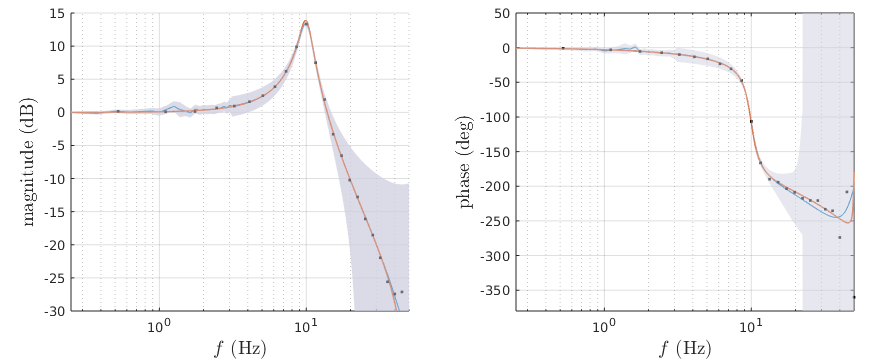
Figure 1: Bode plot of the second-order resonant system (orange), and its estimate (blue) using $H_{\infty}$ Gaussian process regression from an empirical transfer function estimate (black points) with $\eta=3$ confidence ellipsoid bounds (grey).

We apply the strictly-linear $H_{\infty}$ Gaussian process regression method described above to the problem of identifying two second-order systems. The first test system is a second-order system that exhibits a resonance peak. The system is specified in continuous time, with canonical second-order transfer function $g(s)=\frac{\omega_{0}^{2}}{s^{2}+2\xi\omega_{0}s+\omega_{0}^{2}}$, where $\omega_{0}=20\pi$ rad/s, and $\xi=0.1$, and converted to the discrete-time transfer function $g(z)$ using a zero-order hold discretization with a sampling frequency of $f_{s}=100$ Hz. We suppose that we know a priori that there is a resonance peak, but not about its location or half-width, and we have no other strong information about the frequency response. For this prior belief, an appropriate prior model is a weighted mixture of a cozine process and a Hermitian stationary process. In particular, we use the family of $H_{\infty}$ processes with covariance functions $k(z,w)=\sigma^{2}_{g}k_{g}(z,w)+\sigma^{2}_{c}k_{c}(z,w),\tilde{k}(z,w)=\sigma^{2}_{g}\tilde{k}_{g}(z,w)+\sigma^{2}_{c}\tilde{k}_{c}(z,w),$ where $k_{g}$ is the covariance of the geometric $H_{\infty}$ process defined in Example 4.16, and $k_{c}$ is the covariance of the cozine process, and likewise for the complementary covariance. $\sigma^{2}_{g}$ and $\sigma^{2}_{c}$ are weights that determine the relative importance of the two parts of the model. This family of covariances has five hyperparameters: $k_{g}\in[0,\infty)$, $\alpha\in(0,1)$, $k_{c}\in[0,\infty)$, $\omega_{0}\in[0,\pi]$, and $a\in(0,1)$.

We suppose that an input trace $u(n)$ of Gaussian white noise with variance $\sigma^{2}_{u}=1/f_{s}$ is run through $H_{g}$ yielding an output trace $y(n)$; our observations comprise these two traces, corrupted by additive Gaussian white noise of variance $\sigma^{2}=10^{-4}/f_{s}$. To obtain an empirical transfer function estimate, we run both observation traces through a bank of 25 windowed 1000-tap DFT filters. The impulse responses of the filter bank are $h_{i}(n)=e^{j\omega_{i}n}w(n)$ for $i=1,\dotsc,25$, with Gaussian window $w(n)=\exp(-\tfrac{1}{2}(\sigma_{w}(n-500)/1000)^{2})$ for $n=0,\dotsc,999$, and $w(n)=0$ otherwise, with window half-width $\sigma_{w}=0.25$. Let $u_{i}$, $y_{i}$ denote the outputs of filter $h_{i}$ with inputs $u$, $y$ respectively: $y_{i}(n)/u_{i}(n)$ gives a running estimate of $g(e^{j\omega_{i}})$, whose value after 1000 time steps we take as our observation at $z_{i}=e^{j\omega_{i}}$. Figure 1 shows the regression from the strictly linear estimator (34) after tuning the covariance hyperparameters via maximum likelihood, along with predictive error bounds based on $\eta=3$ confidence ellipsoids.

The second is a second-order allpass filter. This system is specified in discrete time with the transfer function $g(z)=\frac{|z_{0}|^{2}-2\ReOp\left[z_{0}\right]+1}{1-2\ReOp\left[z_{0}\right]+|z_{0}|^{2}}$, where $z_{0}=0.5e^{\pm j\pi/4}$ are the system’s poles, with sampling frequency $f_{s}=100$ Hz. For this system we assume that we do not have a priori information on the structure of the frequency response, so we use a Hermitian stationary $H_{\infty}$ process as the prior model. In particular, we take the family of geometric $H_{\infty}$ process, indexed by hyperparameter $\alpha\in(0,1)$. To construct the empirical transfer function estimate, we use the same data model and filter bank as the previous example. Figure 2 shows the strictly linear regression after tuning the covariance hyperparameters, again with predictive error bounds from $\eta=3$ confidence ellipsoids.

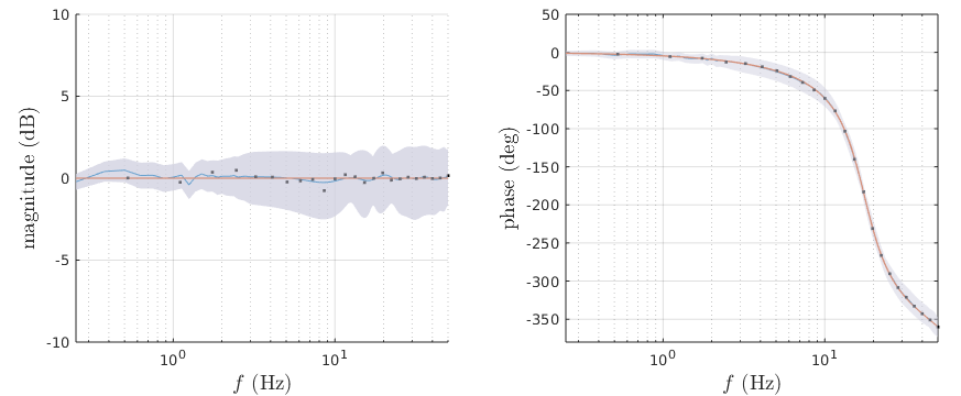
Figure 2: Bode plot of the second-order allpass system (orange), and its estimate (blue) using $H_{\infty}$ Gaussian process regression from an empirical transfer function estimate (black points) with $\eta=3$ confidence ellipsoid bounds (grey).

6 Conclusion

The $H_{\infty}$ processes constructed using the results of this paper, particularly Theorem 4.14, are effective priors for Bayesian nonparametric identification of transfer functions. Furthermore, the strictly linear estimator, which is suboptimal for general complex Gaussian process priors, provides transfer function estimates that are close to optimal for conjugate-symmetric $H_{\infty}$ priors. We have numerical evidence that suggests that as the number of frequency data points increases, the covariance becomes maximally improper, a case in which the strictly linear is indeed optimal. We will investigate this conjecture in future work.

The applications presented in this paper use $H_{\infty}$ Gaussian process as statistically interpretable regression priors, but do not consider questions of probabilistic robustness. We intend to follow this work with a similar investigation into the robustness properties of $H_{\infty}$ models, such as probabilistic bounds on the $H_{\infty}$ norm, and integral quadratic constraints that hold with high probability for an $H_{\infty}$ process with given mean and covariance functions. A simple bound on $\lVert f\rVert_{\infty}$ can be constructed using Borell’s inequality on the real and imaginary parts of $f$, but a bound tight enough for practical use will require more careful analysis.

This work was supported by the grants ONR N00014-18-1-2209, AFOSR FA9550-18-1-0253.

References

- [Adler and Taylor(2007a)] Robert J Adler and Jonathan E Taylor. Random fields and geometry, volume 80. Springer, 2007a.
- [Adler and Taylor(2007b)] Robert J Adler and Jonathan E Taylor. Applications of random fields and geometry: applications and case studies. Unpublished manuscript, 2007b. URL https://robert.net.technion.ac.il/publications/.
- [Balas et al.(2012)Balas, Seiler, and Packard] Gary Balas, Peter Seiler, and Andrew Packard. Analysis of an UAV flight control system using probabilistic . In AIAA Guidance, Navigation, and Control Conference, page 4989, 2012.
- [Biannic et al.(2021)Biannic, Roos, Bennani, Boquet, Preda, and Girouart] Jean-Marc Biannic, Clément Roos, Samir Bennani, Fabrice Boquet, Valentin Preda, and Bénédicte Girouart. Advanced probabilistic -analysis techniques for AOCS validation. European Journal of Control, 62:120–129, 2021.
- [Calafiore and Dabbene(2007)] Giuseppe C Calafiore and Fabrizio Dabbene. Probabilistic robust control. In 2007 American Control Conference, pages 147–158. IEEE, 2007.
- [Chen et al.(2012)Chen, Ohlsson, and Ljung] Tianshi Chen, Henrik Ohlsson, and Lennart Ljung. On the estimation of transfer functions, regularizations and Gaussian processes—revisited. Automatica, 48(8):1525–1535, 2012.
- [Driscoll(1973)] Michael F Driscoll. The reproducing kernel Hilbert space structure of the sample paths of a Gaussian process. Zeitschrift für Wahrscheinlichkeitstheorie und verwandte Gebiete, 26(4):309–316, 1973.
- [Durrett(2019)] Rick Durrett. Probability: theory and examples, volume 49. Cambridge University Press, 2019.
- [Helmberg(1969)] Gilbert Helmberg. Introduction to spectral theory in Hilbert space. North-Holland, 1969.
- [Khatri and Parrilo(1998)] Sven Khatri and Pablo A Parrilo. Guaranteed bounds for probabilistic . In Proceedings of the 37th IEEE Conference on Decision and Control (Cat. No. 98CH36171), volume 3, pages 3349–3354. IEEE, 1998.
- [Khosravi and Smith(2019)] Mohammad Khosravi and Roy S Smith. Kernel-based identification of positive systems. In 2019 IEEE 58th Conference on Decision and Control (CDC), pages 1740–1745. IEEE, 2019.
- [Khosravi and Smith(2021)] Mohammad Khosravi and Roy S Smith. Kernel-based identification with frequency domain side-information. arXiv preprint arXiv:2111.00410, 2021.
- [Landau and Shepp(1970)] Henry J Landau and Lawrence A Shepp. On the supremum of a Gaussian process. Sankhyā: The Indian Journal of Statistics, Series A, pages 369–378, 1970.
- [Lataire and Chen(2016)] John Lataire and Tianshi Chen. Transfer function and transient estimation by Gaussian process regression in the frequency domain. Automatica, 72:217–229, 2016.
- [Paulsen and Raghupathi(2016)] Vern I Paulsen and Mrinal Raghupathi. An introduction to the theory of reproducing kernel Hilbert spaces, volume 152. Cambridge University Press, 2016.
- [Pillonetto and De Nicolao(2010)] Gianluigi Pillonetto and Giuseppe De Nicolao. A new kernel-based approach for linear system identification. Automatica, 46(1):81–93, 2010.
- [Rabiner and Gold(1975)] Lawrence R Rabiner and Bernard Gold. Theory and application of digital signal processing. Englewood Cliffs: Prentice-Hall, 1975.
- [Rasmussen and Williams(2006)] Carl Edward Rasmussen and Christopher K.I. Williams. Gaussian processes for machine learning. MIT Press, 2006.
- [Rudin(1962)] Walter Rudin. Fourier analysis on groups. Interscience, 1962.
- [Schreier and Scharf(2010)] Peter J Schreier and Louis L Scharf. Statistical signal processing of complex-valued data: the theory of improper and noncircular signals. Cambridge University Press, 2010.
- [Singh and Sznaier(2020)] Rajiv Singh and Mario Sznaier. A Loewner matrix based convex optimization approach to finding low rank mixed time/frequency domain interpolants. In 2020 American Control Conference (ACC), pages 5169–5174. IEEE, 2020.
- [Somers et al.(2022)Somers, Thai, Roos, Biannic, Bennani, Preda, and Sanfedino] Franca Somers, Sovanna Thai, Clément Roos, Jean-Marc Biannic, Samir Bennani, Valentin Preda, and Francesco Sanfedino. Probabilistic gain, phase and disk margins with application to AOCS validation. IFAC-PapersOnLine, 55(25):1–6, 2022.
- [Stoddard et al.(2019)Stoddard, Birpoutsoukis, Schoukens, and Welsh] Jeremy G Stoddard, Georgios Birpoutsoukis, Johan Schoukens, and James S Welsh. Gaussian process regression for the estimation of generalized frequency response functions. Automatica, 106:161–167, 2019.
- [Takyar and Georgiou(2010)] Mir Shahrouz Takyar and Tryphon T Georgiou. Analytic interpolation with a degree constraint for matrix-valued functions. IEEE transactions on automatic control, 55(5):1075–1088, 2010.
- [Young(1988)] Nicholas Young. An introduction to Hilbert space. Cambridge University Press, 1988.