Towards More Robust Interpretation via Local Gradient Alignment

Abstract

Neural network interpretation methods, particularly feature attribution methods, are known to be fragile with respect to adversarial input perturbations. To address this, several methods for enhancing the local smoothness of the gradient while training have been proposed for attaining robust feature attributions. However, the lack of considering the normalization of the attributions, which is essential in their visualizations, has been an obstacle to understanding and improving the robustness of feature attribution methods. In this paper, we provide new insights by taking such normalization into account. First, we show that for every non-negative homogeneous neural network, a naive $\ell_{2}$-robust criterion for gradients is not normalization invariant, which means that two functions with the same normalized gradient can have different values. Second, we formulate a normalization invariant cosine distance-based criterion and derive its upper bound, which gives insight for why simply minimizing the Hessian norm at the input, as has been done in previous work, is not sufficient for attaining robust feature attribution. Finally, we propose to combine both $\ell_{2}$ and cosine distance-based criteria as regularization terms to leverage the advantages of both in aligning the local gradient. As a result, we experimentally show that models trained with our method produce much more robust interpretations on CIFAR-10 and ImageNet-100 without significantly hurting the accuracy, compared to the recent baselines. To the best of our knowledge, this is the first work to verify the robustness of interpretation on a larger-scale dataset beyond CIFAR-10, thanks to the computational efficiency of our method.

Introduction

Feature attribution methods (Simonyan, Vedaldi, and Zisserman 2014; Shrikumar, Greenside, and Kundaje 2017; Springenberg et al. 2015; Bach et al. 2015), which refer to interpretation methods that numerically score the contribution of each input feature for a model output, have been useful tools to reveal the behavior of complex models, e.g., deep neural networks, especially in application domains that require safety, transparency, and reliability. However, several recent works (Ghorbani, Abid, and Zou 2019; Dombrowski et al. 2019; Kindermans et al. 2019) identified that such methods are vulnerable to adversarial input manipulation, namely, an adversarially chosen imperceptible input perturbation can arbitrarily change feature attributions without hurting the prediction accuracy of the model. One plausible explanation for this vulnerability can be made from a geometric perspective (Dombrowski et al. 2019), namely, if the decision boundary of a model is far from being smooth, e.g., as in typical neural networks with ReLU activations, a small movement in the input space can dramatically change the direction of the input gradient, which is highly correlated with modern feature attribution methods.

To defend against such adversarial input manipulation, recent approaches (Wang et al. 2020; Dombrowski et al. 2022) regularized the neural network to have locally smooth input gradients while training. A popular criterion to measure the smoothness of the input gradients is to use the $\ell_{2}$-distance between the gradients of the original and perturbed input points, dubbed as the $\ell_{2}$ robust criterion. Since this $\ell_{2}$-criterion can be upper bounded by the norm of the Hessian with respect to the input, (Wang et al. 2020; Dombrowski et al. 2022) used the approximated norm of the Hessian as a regularization term while training. Furthermore, (Dombrowski et al. 2022) shows that replacing the ReLU activation with the Softplus function, Softplus${}_{\beta}(x)=\frac{1}{\beta}\log(1+\exp(\beta x))$, can smooth the decision boundary and lead to a more robust feature attribution method.

While the above approach was shown to be effective to some extent, we argue that only naively considering the $\ell_{2}$ robust criterion is limited since it does not take the normalization of the attributions into account. Such normalization is essential in visualizing the attributions, since the relative difference between the attributions is most useful and important for interpretation. To that end, we argue that simply trying to reduce the $\ell_{2}$ robust criterion or the norm of the Hessian with respect to the input while training may not always lead to robust attributions. As concrete examples, consider the level curves and gradients of four differently trained two-layer neural networks in Figure 1. In Figure 1(a), we clearly observe that the kinks (continuous but not differentiable points) generated by the ReLU activation can cause a dramatic change in the directions of the gradients of two nearby points. In contrast, as shown in Figure 1(b), the Softplus activation smoothes the decision surface, resulting in a less dramatic change of the gradients compared to Figure 1(a) (i.e., smaller $\ell_{2}$ distance and larger cosine similarity). An interesting case is Figure 1(c) that uses the Maximum Entropy (MaxEnt) regularization, which is known to promote a wide-local minimum (Cha et al. 2020) and a small Hessian norm at the trained model parameter, while training. We observe the $\ell_{2}$ distance between the two local gradients has certainly shrunk due to the small norm of the Hessian at the input, but the cosine similarity between them is very low as well; namely, the decrease of the $\ell_{2}$ distance is mainly due to the decrease of the norm of the gradients. Thus, after the normalization of the gradients, the two local gradients still remain very different, leaving the fragility of the interpretation unsolved. This example shows that naively minimizing the Hessian norm as a proxy for robust attribution may not necessarily robustify the attribution methods. An ideal case would be Figure 1(d) in which the $\ell_{2}$ distance is reduced by also aligning the local gradients as we propose in the paper.

In this paper, we propose to develop a more robust feature attribution method, by promoting the alignment of local gradients, hence making the attribution more invariant with respect to the normalization. More specifically, we first define a normalization invariant criterion, which refers to the criterion that has the same value for two functions with the same normalized input gradient. Then, we show that the $\ell_{2}$ robust criterion is not normalization invariant by leveraging the non-negative homogeneous property of the ReLU network. We then suggest considering cosine distance-based criterion and show that it is normalization invariant and is upper bounded by the ratio of the norm of the Hessian and the norm of the gradient at the input. Our theoretical finding explains why simply minimizing the Hessian norm may not necessarily lead to a robust interpretation as in the example of Figure 1(c). Finally, we propose to combine both the $\ell_{2}$ and cosine robust criteria as regularizers while training and show on several datasets and models that our method can achieve promising interpretation robustness. Namely, our method has better robustness with respect to several quantitative metrics compared to other recent baselines and the qualitative visualization for adversarial input also confirmed the robustness of our method. Furthermore, we stress that the computational efficiency of our method enabled the first evaluation of the interpretation robustness on a larger-scale dataset, i.e., ImageNet-100, beyond CIFAR-10.

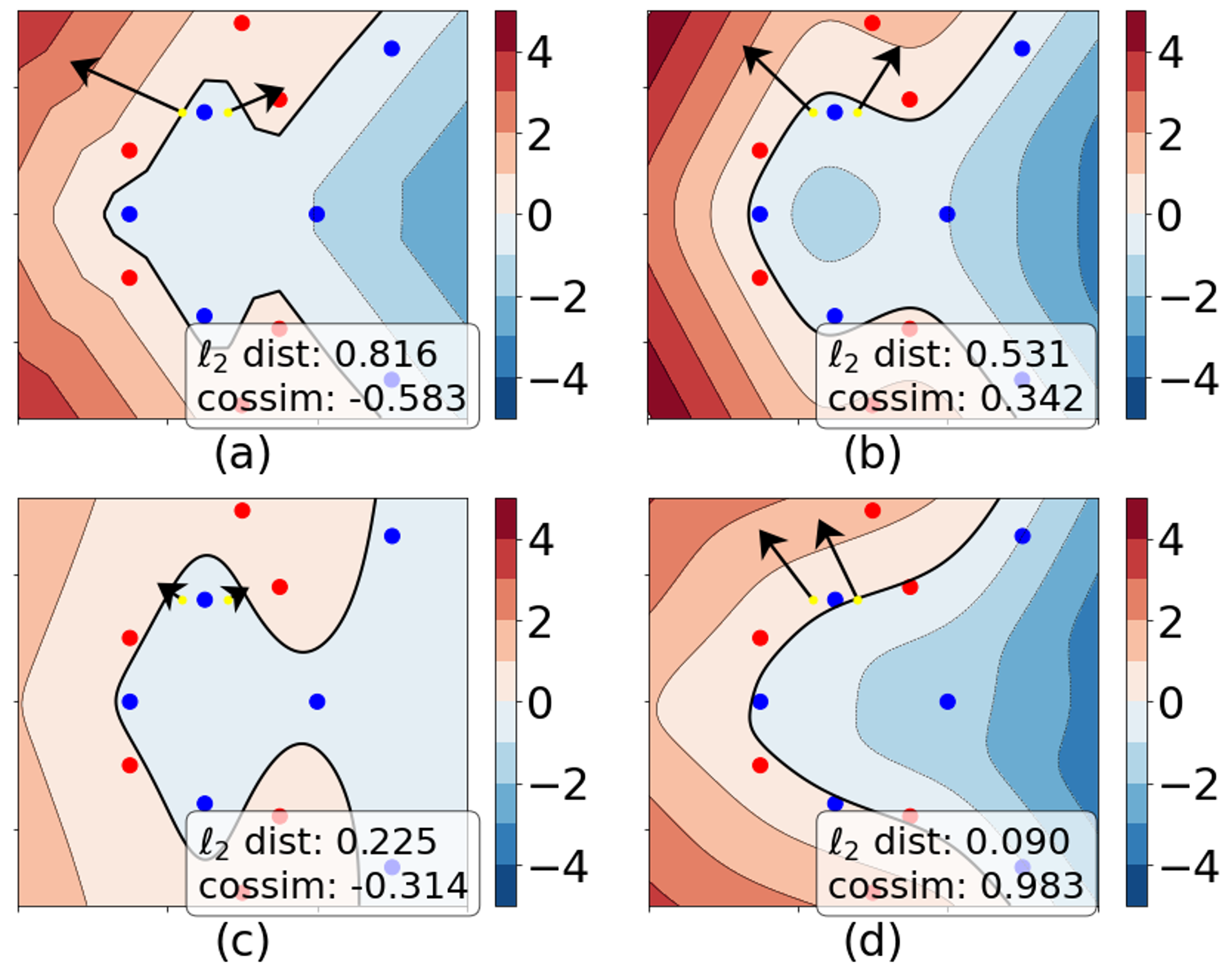
Figure 1: Visualization of the level curves and gradients (shown in arrows) of two nearby input points near the decision boundary of two-layer neural networks, which are trained on a synthetic binary labeled dataset. The $\ell_{2}$ distance and cosine similarities of the two gradient vectors of logit are shown in the legend box. Each figure corresponds to a network trained with (a) ReLU activation with Binary Cross Entropy (BCE) loss. (b) Softplus activation with BCE loss. (c) Softplus activation with BCE loss and a MaxEnt regularizer. (d) Softplus activation with BCE loss and our proposed robust criterion.

Related Works

Vulnerability of attribution methods

Attention toward trustworthy attributions has developed several recent works showing that the attribution methods are susceptible to adversarial or even random perturbations on input or model. (Adebayo et al. 2018; Kindermans et al. 2019; Sixt, Granz, and Landgraf 2020) show that some popular attribution methods generate visually plausible attributes, namely, they are independent of the model or too sensitive to a constant shift to the input. Inspired by adversarial attacks (Goodfellow, Shlens, and Szegedy 2015; Madry et al. 2018), (Ghorbani, Abid, and Zou 2019; Dombrowski et al. 2019) identify that malign manipulation of attributions can be produced by an imperceptible adversarial input perturbation with the same prediction of the model. On the other hand, (Heo, Joo, and Moon 2019; Slack et al. 2020; Lakkaraju and Bastani 2020; Dimanov et al. 2020) changes the model parameters to manipulate the attributions while keeping the model output unchanged.

Towards attribution robustness

Recent efforts toward developing robust attributions have been made from various perspectives. (Rieger and Hansen 2020) suggested that simply aggregating multiple explanation methods can enhance the robustness of attribution. (Anders et al. 2020) proposed a projection-based method that eliminates the off-manifold components in attribution which mainly cause vulnerable attributions. (Smilkov et al. 2017; Si, Chang, and Li 2021) proposed aggregation of explanations over randomly perturbed inputs. The above works have a different focus than ours, since they do not consider model training methodology for attaining robust attributions. Minimization over worst-case input is another well-known strategy for attaining robust attribution. (Chen et al. 2019; Ivankay et al. 2020) suggested adversarial attributional training for an $\ell_{p}$ norm of Integrated Gradient (Sundararajan, Taly, and Yan 2017). Likewise, (Singh et al. 2020) proposed a min-max optimization with soft-margin triplet loss to align input and gradients. However, the inner-maximization process is computationally heavy, which is the main obstacle to applying them in large-scale datasets.

Smoothing the geometry

Smoothing the geometry of the model is a popular approach to building both robust attributions and robust classification. For robust attribution, (Dombrowski et al. 2022; Wang et al. 2020) approximated the norm of the Hessian matrix and regularized it to give a penalty on the principal curvatures. (Tang et al. 2022) proposed knowledge distillation that sample the input by considering the geometry of the teacher model. For adversarial robustness, (Qin et al. 2019) encourages the loss to behave linearly, and (Andriushchenko and Flammarion 2020) reduces cosine distance between gradients of closely located points to prevent catastrophic overfitting that conventionally happens during adversarial training. (Singla et al. 2021; Jastrzebski et al. 2021) analyze how smoothing the curvature can increase adversarial robustness and generalization. Compared to them, our method is the first to apply cosine distance for attaining robust attribution via promoting smooth geometry of the neural networks, with reduced computational complexity.

Preliminaries

Notation

We consider a set of data tuples $\mathcal{D}=\{(\mathbf{x}^{(n)},y^{(n)})\}_{n=1,...,N}$, where $\mathbf{x}^{(n)}\in\mathbb{R}^{d}$ is an input data and $y^{(n)}\in\{1,2,...,C\}$ is the target label. We denote a neural network classifier as $\boldsymbol{g}:\mathbb{R}^{d}\rightarrow\mathbb{R}^{C}$ which returns a logit value for each class. Also, we denote a function $\boldsymbol{p}=\sigma_{\text{softmax}}\circ\boldsymbol{g}:\mathbb{R}^{d}\rightarrow\vartriangle^{C}$ as a composition of the logit and the softmax function that returns a categorical probability, where $\vartriangle^{C}$ denotes a $C$-dimensional simplex. We denote an attribution function by $\mathbf{h}:\mathbb{R}^{d}\rightarrow\mathbb{R}^{d}$, where each element value of $\mathbf{h}$ represents the importance or sensitivity of the input for the output. We always use a bold symbol for vector and vector-valued functions, e.g., $\mathbf{x}$, and $\boldsymbol{g}$, respectively. We use a subscript indexing, e.g., $x_{i}$ is the $i$-th element of a vector $\mathbf{x}$ and $g_{c}$ is a scalar-valued function which returns the $c$-th element of $\boldsymbol{g}(\mathbf{x})$. We denote a scalar-valued function by $f:\mathbb{R}^{d}\rightarrow\mathbb{R}$ and denote a gradient of $f$ with respect to $\mathbf{x}$ by $\nabla f(\mathbf{x})=(\frac{\partial}{\partial x_{1}}f(\mathbf{x}),\frac{\partial}{\partial x_{2}}f(\mathbf{x}),...,\frac{\partial}{\partial x_{d}}f(\mathbf{x}))$. Also, we denote a Hessian matrix of function $f$ with respect to $\mathbf{x}$ by $\mathbf{H}_{f}(\mathbf{x})$, where $(\mathbf{H}_{f}(\mathbf{x}))_{ij}=\frac{\partial^{2}}{\partial x_{i}\partial x_{j}}f(\mathbf{x})$. If there is no ambiguity, we omit the symbol $(n)$ from $(\mathbf{x}^{(n)},y^{(n)})$.

Adversarial attribution manipulation

We first introduce Adversarial Attribution Manipulation (AAM) proposed in (Ghorbani, Abid, and Zou 2019; Dombrowski et al. 2019). The aim of AAM is to find an adversarial example $\mathbf{x}_{\text{adv}}$ in a given $\ell_{p}$ ball around $\mathbf{x}$, $||\mathbf{x}_{adv}-\mathbf{x}||_{p}\leq\epsilon$, such that the attribution changes significantly, while the prediction remains unchanged. The AAM is categorized as targeted, if the goal of the adversary is to make the attribution similar to a target map. In contrast, the AAM is called untargeted, if the adversary makes the attribution as dissimilar as possible compared to the original attribution. The objective of AAM is formally given by

$$\text{minimize}_{||\boldsymbol{\delta}_{\mathbf{x}}||_{p}\leq\epsilon}\Lambda_{\mathbf{h}}(\mathbf{x},\boldsymbol{\delta}_{\mathbf{x}})$$

$$\text{s.t. }\text{argmax}_{c}g_{c}(\mathbf{x}+\boldsymbol{\delta}_{\mathbf{x}})=\text{argmax}_{c}g_{c}(\mathbf{x}),$$

in which $\boldsymbol{\delta}_{\mathbf{x}}\triangleq\mathbf{x}_{adv}-\mathbf{x}$ is an input perturbation and $\Lambda_{\mathbf{h}}(\mathbf{x},\boldsymbol{\delta}_{\mathbf{x}})$ is the attacker’s criterion. In this paper, we mainly consider a targeted AAM proposed in (Dombrowski et al. 2019), in which $\Lambda_{\mathbf{h}}(\mathbf{x},\boldsymbol{\delta}_{\mathbf{x}})=||\mathbf{h}(\mathbf{x}+\boldsymbol{\delta}_{\mathbf{x}})-\mathbf{h}_{t}||_{2}$ is used with $\mathbf{h}_{t}$ being a target map.

To defend against AAM, previous works (Wang et al. 2020; Dombrowski et al. 2022) considered minimizing an $\ell_{2}$ robust criterion which is the $\ell_{2}$ difference between the gradients of logit with respect to closely located points. Formally, the $\ell_{2}$ robust criterion of a function $\boldsymbol{g}$ at a given tuple $(\mathbf{x},y)$ is denoted and defined by

$$\Gamma_{\nabla g_{y}}^{\ell_{2}}(\mathbf{x},\boldsymbol{\delta}_{\mathbf{x}})\coloneqq||\nabla g_{y}(\mathbf{x}+\boldsymbol{\delta}_{\mathbf{x}})-\nabla g_{y}(\mathbf{x})||_{2},$$

where $\boldsymbol{\delta}_{\mathbf{x}}$ is a perturbation. From this definition, we re-write the criterions and their upper bounds that were proposed in (Dombrowski et al. 2022) and (Wang et al. 2020) as

$$\Gamma_{\nabla g_{y}}^{\ell_{2}}(\mathbf{x},\boldsymbol{\delta}_{\mathbf{x}})\leq||\mathbf{H}_{g_{y}}(\mathbf{x})||_{F}L(\mathbf{x}_{adv},\mathbf{x})$$

$$\text{max}_{||\boldsymbol{\delta}_{\mathbf{x}}||_{p}\leq\epsilon}\Gamma_{\nabla\mathcal{L}}^{\ell_{2}}(\mathbf{x},\boldsymbol{\delta}_{\mathbf{x}})\leq\epsilon||\mathbf{H}_{\mathcal{L}}(\mathbf{x})||_{2},$$ (1)

respectively, in which $L(\mathbf{x}_{adv},\mathbf{x})$ is a distance between $\mathbf{x}_{adv}$ to $\mathbf{x}$ and $\mathcal{L}$ denotes a cross-entropy loss. Then, (Wang et al. 2020; Dombrowski et al. 2022) approximated the Hessian and used its norm as a regularizer during training to minimize the upper bound on the $\ell_{2}$ robust criterion.

Remarks 1: Note that the obtained attributions are conventionally normalized, i.e., in case of the vision domain, attribution values are mapped into the range $\{0,...,255\}$ for visualization. Also, the attacker usually normalizes both $\mathbf{h}(\mathbf{x}+\boldsymbol{\delta}_{\mathbf{x}})$ and $\mathbf{h}_{t}$ to match the scale, because $\mathbf{h}_{t}\in\{0,1\}^{d}$ in usual, while $\mathbf{h}(\mathbf{x}+\boldsymbol{\delta}_{\mathbf{x}})$ has a much diverse range.
Remarks 2: If a neural network is a piece-wise linear function, the Hessian matrix of logit $\mathbf{H}_{g_{c}}(\mathbf{x})$ is a zero matrix. To make Hessian non-zero, (Wang et al. 2020; Moosavi-Dezfooli et al. 2019) considered the Hessian of the cross entropy loss, instead of the logit function. However, this alternative would still contain non-differentiable points. On the other hand, (Dombrowski et al. 2022) introduced a Dirac delta function to deal with a non-differentiable point, i.e., ReLU${}^{\prime\prime}(x)=\delta(x)$. Besides, (Ghorbani, Abid, and Zou 2019) considered replacing the ReLU with Softplus, which is twice differentiable and well approximates ReLU.

Theoretical Consideration

Normalization invariant criterion

As we described in Figure 1, the reduction of the $\ell_{2}$ robust criterion or Hessian norm may not always lead a model to be robust against the AAM, because such reduction can be also achieved by decreasing the norms of the gradients without actually aligning them. Such limitation of the $\ell_{2}$ criterion motivates us to devise a criterion that would not be affected by the normalization of the gradient. We formally define a normalization invariant criterion as follows.

Definition 1.

For given functions $\boldsymbol{f}:\mathbb{R}^{d}\rightarrow\mathbb{R}^{C}$ and $\boldsymbol{g}:\mathbb{R}^{d}\rightarrow\mathbb{R}^{C}$ that satisfy $\nabla f_{y}(\mathbf{x})/||\nabla f_{y}(\mathbf{x})||_{2}=\nabla g_{y}(\mathbf{x})/||\nabla g_{y}(\mathbf{x})||_{2}$ for all $(\mathbf{x},y)\in\mathbb{R}^{d}\times\{1,2,...,C\}$, a criterion $\Gamma$ is called normalization invariant (for $\boldsymbol{f}$ & $\boldsymbol{g}$), if

$$\Gamma_{\nabla f_{y}}(\mathbf{x},\boldsymbol{\delta}_{\mathbf{x}})=\Gamma_{\nabla g_{y}}(\mathbf{x},\boldsymbol{\delta}_{\mathbf{x}}),$$

in which $\Gamma_{f}(\mathbf{x},\boldsymbol{\delta}_{\mathbf{x}})$ stands for some function that measures the distance between $f(\mathbf{x})$ and $f(\mathbf{x}+\boldsymbol{\delta}_{\mathbf{x}})$.

Next, we show that the $\ell_{2}$ robust criterion $\Gamma_{\nabla f}^{\ell_{2}}$ is not normalization invariant for any neural network of which the final layer is a fully connected layer. Without loss of generality, we denote a set of parameters for a neural network as $\Theta=\{\boldsymbol{\theta}_{1},\boldsymbol{\theta}_{2},...,\boldsymbol{\theta}_{L}\}$, where each $\boldsymbol{\theta}_{i}$ refers to the parameter of the $i$-th layer. We define an $\alpha$-transformation as $T_{i}(\Theta,\alpha)=\{\boldsymbol{\theta}_{1},...,\boldsymbol{\theta}_{i-1},\alpha\boldsymbol{\theta}_{i},\boldsymbol{\theta}_{i+1},...,\boldsymbol{\theta}_{L}\}$ which scales the $i$-th parameter by $\alpha>0$. Then, we define a notion of non-negative homogeneous function as follows.

Definition 2.

A function $\boldsymbol{f}:\mathbb{R}^{d}\to\mathbb{R}^{C}$ with parameters $\Theta=\{\boldsymbol{\theta}_{1},\boldsymbol{\theta}_{2},...,\boldsymbol{\theta}_{L}\}$ is non-negative homogeneous with respect to parameter $\boldsymbol{\theta}_{i}$, if $\boldsymbol{f}$ satisfies the following for all $\alpha\in\mathbb{R_{+}}$ and $\mathbf{x}\in\mathbb{R}^{d}$:

$$\boldsymbol{f}(\mathbf{x};T_{i}(\Theta,\alpha))=\alpha\boldsymbol{f}(\mathbf{x};\Theta).$$

We note that every neural network with the final fully-connected layer is non-negative homogeneous with respect to the parameters of the last layer. Moreover, a feed-forward neural network with ReLU activation can be shown to be non-negative homogeneous, with respect to any parameters, of which proofs are available in Appendix B. Now, we show the following lemma on the $\ell_{2}$ robust criterion for non-negative homogeneous neural networks.

Lemma 3.

The $\ell_{2}$ robust criterion is not normalization invariant for non-negative homogeneous neural networks.

Proof: Let $\boldsymbol{g}$ be the non-negative homogeneous neural network. Then, for any output class $c$, by performing the $\alpha$-transformation, we can set $f(\mathbf{x})=\alpha g_{y}(\mathbf{x})$ for any $\alpha\in\mathbb{R}_{+}$ and $\mathbf{x}\in\mathbb{R}^{d}$. Then, it is clear that $\nabla g_{y}(\mathbf{x})/||\nabla g_{y}(\mathbf{x})||_{2}=\alpha\nabla g_{y}(\mathbf{x})/||\alpha\nabla g_{y}(\mathbf{x})||_{2}=\nabla f(\mathbf{x})/||\nabla f(\mathbf{x})||_{2},$ but we have

$$\Gamma_{\nabla f}^{\ell_{2}}(\mathbf{x},\boldsymbol{\delta}_{\mathbf{x}}) =||\nabla f(\mathbf{x}+\boldsymbol{\delta}_{\mathbf{x}})-\nabla f(\mathbf{x})||_{2}$$

$$=\alpha||\nabla g_{y}(\mathbf{x}+\boldsymbol{\delta}_{\mathbf{x}})-\nabla g_{y}(\mathbf{x})||_{2}$$

$$=\alpha\cdot\Gamma_{\nabla g_{y}}^{\ell_{2}}(\mathbf{x},\boldsymbol{\delta}_{\mathbf{x}}).$$ (2)

Therefore, $f$ and $g_{y}$ can have different $\ell_{2}$ criterion values although they have the same normalized gradient. ∎

The above lemma implies that minimizing the $\ell_{2}$ robust criterion for non-negative homogeneous neural networks may not be satisfactory for obtaining robust interpretations. The reason is that it may simply result in scaling the network parameters such that the criterion is minimized, but the argmax prediction and the gradient direction for the network remain unchanged.

A cosine robust criterion

From the result of the previous section, we propose cosine robust criterion (CRC) which measures the cosine distance between the gradients at two nearby points.

Definition 4.

A cosine robust criterion of a function $\boldsymbol{g}$ at point $(\mathbf{x},y)$ is denoted and defined by

$$\Gamma_{\nabla g_{y}}^{\text{\emph{cos}}}(\mathbf{x},\boldsymbol{\delta}_{\mathbf{x}})\coloneqq\frac{1}{2}\big{(}1-\text{cossim}\left(\nabla g_{y}(\mathbf{x}+\boldsymbol{\delta}_{\mathbf{x}}),\nabla g_{y}(\mathbf{x})\right)\big{)},$$

in which $\text{cossim}(\mathbf{v},\mathbf{w})=\mathbf{v}^{T}\mathbf{w}/(||\mathbf{v}||_{2}\cdot||\mathbf{w}||_{2})$.

Proposition 5.

The cosine robust criterion is normalization invariant for any $\boldsymbol{f}$ and $\boldsymbol{g}$ that satisfies $\nabla f_{y}(\mathbf{x})/||\nabla f_{y}(\mathbf{x})||_{p}=\nabla g_{y}(\mathbf{x})/||\nabla g_{y}(\mathbf{x})||_{p}$ for all $(\mathbf{x},y)$.

The proof of Proposition 5 is trivial because the normalization is self-contained in the cosine similarity. We now attain the upper bound on CRC as follows.

Theorem 6.

For a twice differentiable function $g$, $\epsilon>0$ with $\epsilon\ll 1$, and $\forall(\mathbf{x},\boldsymbol{\delta}_{\mathbf{x}})\in\mathbb{R}^{d}\times\mathbb{R}^{d}$, we have

$$\Gamma_{\nabla g}^{\text{\emph{cos}}}(\mathbf{x},\epsilon\boldsymbol{\hat{\delta}}_{\mathbf{x}})\leq\frac{\epsilon\|\mathbf{H}_{g}(\mathbf{x})\|_{F}+\mathcal{O}(\epsilon^{2})}{\|\nabla g(\mathbf{x}+\epsilon\boldsymbol{\hat{\delta}}_{\mathbf{x}})\|_{2}},$$ (3)

in which $\boldsymbol{\hat{\delta}}_{\mathbf{x}}=\boldsymbol{\delta}_{\mathbf{x}}/||\boldsymbol{\delta}_{\mathbf{x}}||_{2}$.

Proof: See Appendix B. ∎

In the theorem, without loss of generality, we substituted $\boldsymbol{\delta}_{\mathbf{x}}$ in the CRC with a multiplication of scalar and unit vector, denoted as $\epsilon\boldsymbol{\hat{\delta}}_{\mathbf{x}}$, and we applied the Taylor expansion $\nabla g(\mathbf{x}+\epsilon\boldsymbol{\hat{\delta}}_{\mathbf{x}})=\nabla g(\mathbf{x})+\epsilon\mathbf{H}_{g}(\mathbf{x})\boldsymbol{\hat{\delta}}_{\mathbf{x}}+\mathcal{O}(\epsilon^{2})\mathbf{v}$. This theorem implies that only minimizing the Hessian norm as in (Wang et al. 2020; Dombrowski et al. 2022) may not be sufficient to align the local gradients, i.e., minimize the CRC. As a simple example, consider again a non-negative homogeneous neural network $\boldsymbol{g}$ that can be $\alpha$-transformed into $f(\mathbf{x})=\alpha g_{y}(\mathbf{x})$ for any output class $y$ as in the proof of Lemma 3. Then, we observe that the Hessian norm of $f$ can be easily minimized since $\|\mathbf{H}_{f}(\mathbf{x})\|_{2}=\alpha\|\mathbf{H}_{g_{y}}(\boldsymbol{g})\|_{2}$ and $\alpha$ can be made arbitrarily small. However, since we also have $\|\nabla f(\mathbf{x})\|_{2}=\alpha\|\nabla g_{y}(\mathbf{x})\|_{2}$ for any $\mathbf{x}$, the upper bound in (3) would not shrink for $f$, showing that a simple $\alpha$-transformation of a non-negative homogeneous neural network would not necessarily minimize CRC as opposed to the $\ell_{2}$ robust criterion in Lemma 3.

Proposing Methods

From the theoretical considerations of the previous section, we may first propose a straightforward way to directly apply the CRC to training. Namely, for a single data tuple $(\mathbf{x},y)$ and model $\boldsymbol{g}$, we denote a training loss function with regularization as $\mathcal{L}(\mathbf{x},y)$ and define it as

$$\mathcal{L}(\mathbf{x},y)=\mathcal{L}_{CE}(\mathbf{x},y)+\lambda_{\text{cos}}\mathbb{E}_{\boldsymbol{\delta}_{\mathbf{x}}}\Big{[}\Gamma_{\nabla g_{y}}^{\text{cos}}(\mathbf{x},\boldsymbol{\delta}_{\mathbf{x}})\Big{]},$$ (4)

in which $\mathcal{L}_{CE}(\mathbf{x},y)$ is the cross-entropy loss, $\boldsymbol{\delta}_{\mathbf{x}}$ is sampled from $\mathcal{U}_{d}([-\epsilon,\epsilon]^{d})$, a $d$-dimensional multivariate uniform distribution on an $\ell_{\infty}$ $\epsilon$-ball, and $\lambda_{\text{cos}}$ is a hyper-parameter for determining the CRC regularization strength.

While using CRC as a regularizer seems promising in the sense of maintaining similar directions for local gradients, we argue that only considering the angle between local gradients by CRC might cause instability while training and large variability of the magnitude of the gradients. An extreme case that could occur in training is that we enforce a similar derivative direction in a ball around $\mathbf{x}$, but as we move in some direction from $\mathbf{x}$ towards the edge of the ball, the magnitude of the derivative could become very low. In this case, if we were to continue in the same direction just beyond the edge of the ball, the direction of the derivative could flip and point in the opposite direction. This phenomenon may reduce training stability and generalization of behavior beyond the training points.

With the above reasoning, our final proposal is to combine both cosine and $\ell_{2}$ robust criteria as regularizers:

$$\mathcal{L}(\mathbf{x},y)=\mathcal{L}_{CE}(\mathbf{x},y)$$

$$+\mathbb{E}_{\boldsymbol{\delta}_{\mathbf{x}}}\Big{[}\lambda_{\text{cos}}\Gamma_{\nabla g_{y}}^{\text{cos}}(\mathbf{x},\boldsymbol{\delta}_{\mathbf{x}})+\lambda_{\ell_{2}}\Gamma_{\nabla g_{y}}^{\ell_{2}}(\mathbf{x},\boldsymbol{\delta}_{\mathbf{x}})\Big{]},$$ (5)

in which $\lambda_{\ell_{2}}$ is a hyper-parameter for the $\ell_{2}$ regularization strength, and $\boldsymbol{\delta}_{\mathbf{x}}$ is again sampled from $\mathcal{U}_{d}([-\epsilon,\epsilon]^{d})$. Both regularizers complement each other: the CRC helps to align the local gradients, while the $\ell_{2}$ regularizer contributes to stable training steps. For every training iteration, we do a Monte-Carlo sampling for each data point to sample $\boldsymbol{\delta}_{\mathbf{x}}$. While we do not consider the worst-case perturbation as in adversarial training (Madry et al. 2018), we instead try to align the local gradients within the $\ell_{\infty}$ $\epsilon$-ball to achieve probable robustness.

Experiments

Attribution methods

We measure the robustness of attribution methods that are known to be closely related to the input gradient, i.e., Gradient, Input$\times$Gradient, Guided Backprop, and LRP. These methods generate saliency maps, showing which pixels are most relevant to the classifier output. We denote the saliency map for model $\boldsymbol{g}$ at data tuple $(\mathbf{x},y)$ using attribution method $\mathcal{I}$ as $\mathbf{h}_{g_{y}}^{\mathcal{I}}(\mathbf{x})$.

Gradient (Simonyan, Vedaldi, and Zisserman 2014): This method is defined by $\mathbf{h}_{g_{y}}^{\text{Grad}}(\mathbf{x})=\nabla g_{y}(\mathbf{x})$, which is the gradient of a logit with respect to input.

Input$\times$Gradient (Shrikumar, Greenside, and Kundaje 2017): This method calculates the element-wise multiplication of input and gradient, $\mathbf{h}_{g_{y}}^{\times\text{Grad}}(\mathbf{x})=\mathbf{x}\odot\nabla g_{y}(\mathbf{x})$.

Guided Backprop (Springenberg et al. 2015): This method is a modified back-propagation method that does not propagate the true gradient, but the imputed gradient when it passes through the activation function. Specifically, if the forward pass of the activation is given by $a_{i}=\text{max}(z_{i},0)$, the modified propagation is represented as $\nabla_{z_{i}}g_{y}=\nabla_{a_{i}}g_{y}\cdot\mathbf{1}(\nabla_{a_{i}}g_{y}>0)\cdot\mathbf{1}(z_{i}>0)$. We denote this method as $\mathbf{h}_{g_{y}}^{GBP}$.

LRP (Bach et al. 2015): LRP propagates relevance from output to input layer-by-layer, based on the contributions of each layer. We used the z+ box rule in our experiments, as adopted in (Dombrowski et al. 2022). Starting from the relevance score of the output layer $R_{i}^{(L)}=\delta_{iy}$, we apply the $z^{+}$ propagation rule for the intermediate layers

$$R_{i}^{(\ell)}=\sum_{j}\frac{x_{i}^{(\ell)}(W_{ij}^{(\ell)})_{+}}{\sum_{i^{\prime}}x_{i^{\prime}}^{(\ell)}(W_{i^{\prime}j}^{(\ell)})_{+}}R_{j}^{(\ell+1)},$$

where $\mathbf{W}^{(\ell)}$ and $x_{i}^{(\ell)}$ denote the weights and activation vector of the $\ell$-th layer, respectively. For the last layer, we use the $z^{\mathcal{B}}$ rule to bound the relevance score in the input domain,

$$R_{i}^{(0)}=\sum_{j}\frac{x_{i}^{(0)}W_{ij}^{(0)}-l_{i}(W_{ij}^{(0)})_{+}-h_{i}(W_{ij}^{(0)})_{-}}{\sum_{i^{\prime}}x_{i^{\prime}}^{(0)}W_{i^{\prime}j}^{(0)}-l_{i^{\prime}}(W_{i^{\prime}j}^{(0)})_{+}-h_{i^{\prime}}(W_{i^{\prime}j}^{(0)})_{-}}R_{j}^{(1)},$$

where $l_{i}$ and $h_{i}$ are the lower and upper bounds of the input domain. The heatmap is then denoted as $\mathbf{h}^{LRP}_{g_{y}}(\mathbf{x})=\mathbf{R}^{(0)}$.

Table 1: Quantitative results

Dataset Model	Regularizer	Accuracy	Grad (2014)			xGrad (2017)			GBP (2015)			LRP (2015)
			RPS	Ins	A-Ins	RPS	Ins	A-Ins	RPS	Ins	A-Ins	RPS	Ins	A-Ins
CIFAR10 LeNet	CE only	86.8	0.760	35.5	29.1	0.749	43.1	37.4	0.897	51.0	43.0	0.980	56.6	48.4
	ATEX (Tang et al. 2022)	88.0	0.771	35.0	28.9	0.760	43.0	37.5	0.907	51.5	42.7	0.982	58.0	49.9
	IGA (Singh et al. 2020)	86.3	0.837	37.9	34.0	0.822	47.2	44.6	0.937	57.7	54.7	0.994	59.1	55.1
	Hessian (Dombrowski et al. 2022)	86.3	0.872	37.6	31.7	0.861	45.8	41.6	0.960	59.4	54.8	0.993	59.2	56.3
	$\ell_{2}$	86.4	0.881	41.1	33.4	0.873	48.2	42.3	0.963	59.5	55.4	0.992	59.9	56.5
	$\ell_{2}$+ Cosd (ours)	86.1	0.895	43.3	35.8	0.887	50.5	44.8	0.966	61.4	57.4	0.992	60.3	57.1
CIFAR10 ResNet18	CE only	94.0	0.724	40.8	31.7	0.708	47.7	39.6	0.902	60.1	53.8	0.972	64.5	59.8
	Hessian (Dombrowski et al. 2022)	93.3	0.864	46.6	38.3	0.852	53.9	48.0	0.961	62.3	57.7	0.988	70.3	68.3
	$\ell_{2}$	93.3	0.908	49.3	43.3	0.898	56.7	52.2	0.976	65.9	65.1	0.988	71.1	70.3
	$\ell_{2}$+ Cosd (ours)	93.0	0.931	53.4	48.9	0.924	58.7	55.3	0.974	66.1	65.1	0.989	70.8	69.7
ImageNet100 ResNet18	CE only	79.0	0.790	39.8	29.8	0.777	44.7	34.1	0.909	49.1	34.0	0.948	50.1	35.3
	Hessian (Dombrowski et al. 2022)	78.9	0.830	42.4	33.6	0.816	46.5	37.5	0.886	48.7	36.4	0.947	49.3	38.9
	$\ell_{2}$	78.0	0.913	44.2	35.4	0.903	48.0	39.4	0.956	48.9	40.9	0.970	49.8	40.8
	$\ell_{2}$+ Cosd (ours)	78.0	0.942	45.2	37.0	0.934	49.0	41.1	0.971	49.0	42.5	0.976	50.9	43.3

Experimental settings

We used the CIFAR10 (Krizhevsky and Hinton 2009) and ImageNet100 (Shekhar 2021; Russakovsky et al. 2015) datasets to evaluate the robustness of our proposed regularization methods. The ImageNet100 dataset is a subset of the ImageNet-1k dataset with 100 of the 1K labels selected. The train and test dataset contains 1.3K and 50 images for each class, respectively. We choose a three-layer custom convolutional neural network (LeNet) and ResNet18 (He et al. 2016) for our experiments since our objective is not to achieve state-of-the-art accuracy for those datasets, but to evaluate the robustness of interpretation for popular models. We replaced all ReLU activations with Softplus$(\beta=3)$ as given by (Dombrowski et al. 2019), which makes the Hessian non-zero, as well as allows the model to have smoother geometry. We set Adversarial Training on EXplanation (ATEX) (Tang et al. 2022), triplet-based Input Gradient Alignment (IGA) (Singh et al. 2020), approximated norm of Hessian (Dombrowski et al. 2022), $\ell_{2}$ robust criterion as our baselines. Our method is denoted by $\ell_{2}+$Cosd. We performed a grid search for selecting hyperparameters. For each hyperparameter, we trained the model three times from scratch and reported the mean value in Appendix C. Our code is available at https://github.com/joshua840/RobustAGA.

Training details

We applied two tricks to speed up our training. First, we sampled $\boldsymbol{\delta}_{\mathbf{x}}$ only once per iteration. Second, before calculating $\Gamma_{\nabla g_{y}}^{\ell_{2}}(\mathbf{x},\boldsymbol{\delta}_{\mathbf{x}})$ and $\Gamma_{\nabla g_{y}}^{\text{cos}}(\mathbf{x},\boldsymbol{\delta}_{\mathbf{x}})$ in (5), we treat $\nabla g_{y}(\mathbf{x})$ as constant to prevent the gradient flows during back-propagation. The gradient of the regularization term is still propagated through $\nabla g_{y}(\mathbf{x}+\boldsymbol{\delta}_{\mathbf{x}})$. We verified that the second technique accelerates the training speed by approximately 25%, while there are no significant differences in the prediction accuracy and attribution robustness.

Metrics

Random perturbation similarity

We employ random perturbation similarity (RPS) (Dombrowski et al. 2022), which measures the similarity of the attribution at the given point $\mathbf{x}$ and the randomly perturbed point $\mathbf{x}+\boldsymbol{\delta}_{\mathbf{x}}$. Formally, for given dataset $\mathcal{D}$, model $\boldsymbol{g}$, metric $\mathcal{S}$, attribution method $\mathcal{I}$, and noise level $\epsilon$, the RPS is defined as

$$RP S_{\boldsymbol{g}}(\mathcal{S},\mathcal{I},\epsilon,\mathcal{D})$$

$$=\frac{1}{N}\sum_{(\mathbf{x},y)\in\mathcal{D}}\mathbb{E}_{\boldsymbol{\delta}_{\mathbf{x}}\sim\mathcal{U}_{d}([-\epsilon,\epsilon]^{d})}\mathcal{S}(\mathbf{h}_{g_{y}}^{\mathcal{I}}(\mathbf{x}+\boldsymbol{\delta}_{\mathbf{x}}),\mathbf{h}_{g_{y}}^{\mathcal{I}}(\mathbf{x})),$$

in which $N$ is the number of data tuples in $\mathcal{D}$ and $\mathcal{U}_{d}$ denotes the uniform distribution. We performed Monte-Carlo sampling 10 times for each data tuple to approximate the expectation over $\boldsymbol{\delta}_{\mathbf{x}}$. We set $\epsilon$ as 4, 8, and 16. We employ cosine similarity, Pearson Correlation Coefficient (PCC), and Structural SIMilarity (SSIM) for the similarity metric $\mathcal{S}$, where PCC and SSIM are also used in previous literature (Dombrowski et al. 2022; Adebayo et al. 2018). We will omit the $\boldsymbol{g}$ and $\mathcal{D}$ for simplicity.

Insertion and Adv-Insertion game

Another well-known strategy to measure the quality of attribution is to reconstruct the input pixels and observe the changes in output. We employed the Insertion game (Petsiuk, Das, and Saenko 2018), which observes the changes in categorical probability for the true label $y$ by inserting the input in the order of attribution score. In detail, we reconstruct the $\gamma$ ratio of input elements from the zero-valued image $\mathbf{x}_{o}$, in the order of the interpretation score $\mathbf{h}_{g_{y}}^{\mathcal{I}}(\mathbf{x})$. To do this, we build a mask vector $\mathbf{m}_{\gamma}^{\mathcal{I}}\in\{0,1\}^{d}$ such that each element satisfies $(\mathbf{m}_{\gamma}^{\mathcal{I}})_{i}=\mathbf{1}[(\mathbf{h}_{g_{y}}^{\mathcal{I}}(\mathbf{x}))_{i}>t_{\gamma}]$ and $\sum_{i}(\mathbf{m}_{\gamma}^{\mathcal{I}})_{i}/d=\gamma$ by carefully choosing the threshold $t_{\gamma}$. We denote the reconstructed input as $\mathbf{x}_{\gamma}^{\mathcal{I}}$ and define as $\mathbf{x}_{\gamma}^{\mathcal{I}}=\mathbf{x}\odot\mathbf{m}_{\gamma}^{\mathcal{I}}+\mathbf{x}_{o}\odot(\mathbf{1-m}_{\gamma}^{\mathcal{I}})$. Then, the average probability after insertion is defined as:

$$\text{Insertion}_{\boldsymbol{g}}(\mathcal{I},\mathcal{D},\gamma) =\frac{1}{N}\sum_{(\mathbf{x},y)\in\mathcal{D}}p_{y}(\mathbf{x}_{\gamma}^{\mathcal{I}}).$$

We also propose Adv-Insertion to measure the robustness of attributions against AAM. The overall process of Adv-Insertion is similar to normal Insertion, but Adv-Insertion determines the order of the input reconstruction by $\mathbf{h}_{g_{y}}^{\mathcal{I}}(\mathbf{x}_{adv})$, where the $\mathbf{x}_{adv}$ is derived from targeted AAM. The A-Ins score will be high if the manipulated attribution $\mathbf{h}_{g_{y}}^{\mathcal{I}}(\mathbf{x}_{adv})$ still well reflects the model behavior. For AAM in our experiments, we used PGD-$\ell_{\infty}(iter=100)$ where $\epsilon=2/255$ for ResNet18 and $\epsilon=4/255$ for LeNet. Also, we selected $\mathbf{h}_{t}$ as a frame image as shown in Figure 3(a) to minimize the overlap between the class object and target map. We calculated Insertion and Adv-Insertion for each $\gamma\in\{0,0.05,...,0.95,1\}$ and posted the mean values over the reconstruction ratio $\gamma$.

Quantitative and qualitative results

Table 1 shows quantitative results for four attribution methods and three robustness metrics. We denoted Insertion and Adv-Insertion as Ins and A-Ins, respectively. We selected hyperparameters that have the highest RPS on the Grad attribution while allowing 1% of test accuracy drops from CE only (without attribution regularization).For RPS, we only posted cosine similarity with $\epsilon=16$ results. All of the other results including cosine similarity, PCC, and SSIM with $\epsilon=4,8,16$, and the other hyperparameters are given in Appendix C. Note that we did not evaluate the results for IGA and ATEX in ResNet18 since they have high computational costs.

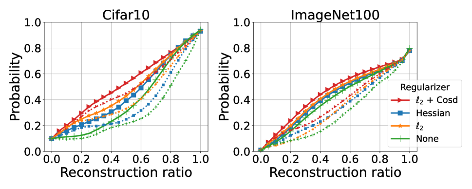
(a) Insertion (solid line) and Adv-Insertion (dotted line) curves for CIFAR10 and ImageNet. ResNet18 and Grad explanation are used for both graphs.

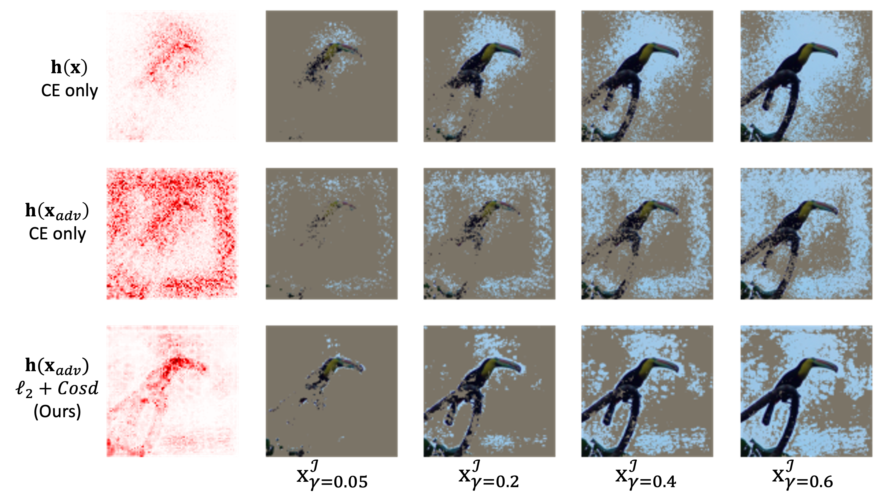
(b) Examples of reconstructed images that are used in the Insertion and Adv-Insertion metrics. Column 1: Visualizations of Grad explanation, which determines the reconstruction order. Column 2 $\sim$ 5: Reconstructed images where $\gamma=\{0.05,0.2,0.4,0.6\}$.

Figure 2: Insertion and Adv-Insertion metrics.

Robustness on the random perturbation

Overall, our method shows the highest RPS on CIFAR10 and ImageNet100 for almost all attribution methods, which underscores that the model trained by our method has smoother geometry on average than the other methods. In the case of ATEX, the self-knowledge distillation gives high accuracy gain but the robustness of the attribution is poor. Interestingly, our method has better robustness results than IGA, which is computationally expensive with inner maximization computations. Also, it turns out that ATEX, IGA, and Hessian are worse than not only our method but also the method with only $\ell_{2}$, which needs much less computation time and memory.

Insertion and Adv-Insertion

Our Insertion and Adv-Insertion game results are given in both Table 1 and Figure 2. In Table 1, the model trained by our method achieves the best or comparable Insertion and Adv-Insertion scores. The tendency of Adv-Insertion is similar for different values of the $\epsilon$, which are given in Appendix C. Especially, the Adv-Insertion score of the model trained on CIFAR10-ResNet18 with our method is comparable to the Insertion score of the model trained with $\ell_{2}$ regularization, which highlights the robustness of our method against the adversarial input. In Figure 2(a), we can observe that our $\ell_{2}$+Cosd method has the highest probability all over the reconstruction ratio. Qualitatively, Figure 2(b) shows that the main object part is well preserved in the reconstructed image for our method since $\mathbf{h}(\mathbf{x}_{adv})$ still mainly highlights the main object even for the adversarial input, in contrast to the CE only training.

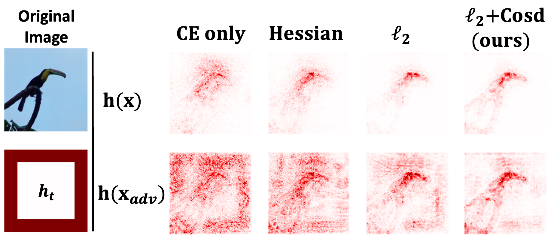
(a) Attribution Visualization

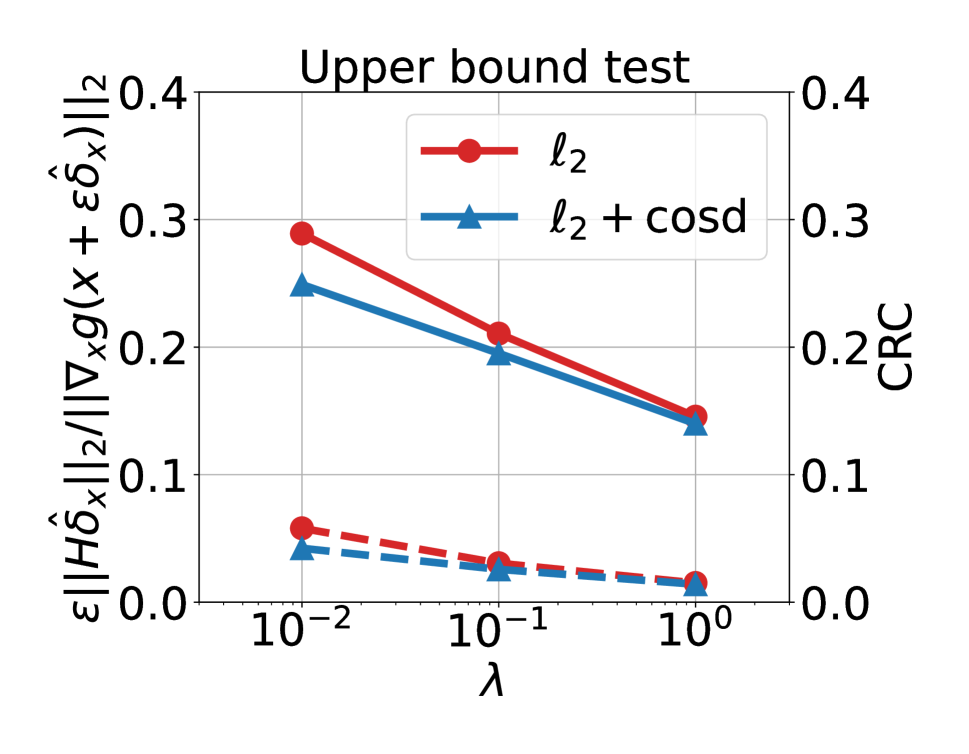
(b) Upper bound test

Figure 3: (a) Row 1: Visualization of attribution maps for each of the four different models, CE only, Hessian, $\ell_{2}$ and $\ell_{2}$ + Cosd. Row 2: Adversarially attacked images, i.e., $\mathbf{x}_{adv}$ with targeted AAM with $\mathbf{h}_{t}$, are made and the attacked attribution maps are generated for each model. (b) Solid: Upper bound in (3) without the $\mathcal{O}(\epsilon^{2})$ term, Dotted: CRC in Def.4.

Qualitative results

Figure 3(a) shows saliency map visualization. We visualize the Grad attributions for both the source image $\mathbf{x}$ and the manipulated images $\mathbf{x}_{adv}$, where $\mathbf{x}_{adv}$ is derived from targeted AAM with PGD-${\ell_{\infty}}(\epsilon=2/255,iter=100)$ applied. The attribution of the manipulated image with our proposed method shows a much more robust appearance than those with the other methods using only Hessian or $\ell_{2}$; i.e., ours shows attribution that is clearly sparse and highlights the main object, while others include the spurious target attribution $h_{t}$.

Table 2: Training complexity

	CIFAR10 LeNet		CIFAR10 ResNet18		ImageNet100 ResNet18
Regularizer	Time	Memory	Time	Memory	Time	Memory
CE only	$\times$ 1.0	$\times$ 1.0	$\times$ 1.0	$\times$ 1.0	$\times$ 1.0	$\times$ 1.0
Hessian	$\times$ 4.25	$\times$ 4.36	$\times$ 8.95	$\times$ 6.62	$\times$ 13.88	$\times$ 4.06
ATEX $(3^{rd}$ step)	$\times$ 2.25	$\times$ 2.81	$\times$ 2.22	$\times$ 3.16	-	-
IGA	$\times$ 31.0	$\times$ 6.55	$\times$ 26.45	$\times$ 6.74	-	-
$\ell_{2}$+Cosd (ours)	$\times$ 2.75	$\times$ 2.64	$\times$ 4.10	$\times$ 2.65	$\times$ 4.94	$\times$ 2.19

Discussion

Upper bounds

In Figure 3(b), we plot $\frac{\epsilon||\mathbf{H}_{g}(\mathbf{x})\boldsymbol{\hat{\delta}}_{\mathbf{x}}||_{2}}{||\nabla g(\mathbf{x}+\epsilon\boldsymbol{\hat{\delta}}_{\mathbf{x}})||_{2}}$, a slightly tighter term than what is given as an upper bound in Equation 3, and the cosine distance for models that trained with $\ell_{2}$ and $\ell_{2}$+Cosd on the CIFAR10-LeNet. The figure shows that the upper bound on CRC is well aligned with the cosine distance.

Training speed

Table 2 shows the memory and time requirements of the regularization methods used in Table 1. We set the CE-only model as $\times$1 and reported the relative time and memory consumption. Our method is much more efficient than the other regularization methods, from both time and memory perspectives. Note that ATEX has three steps, but we only measured the time and accuracy for the third step.

Second order derivatives

Hessian regularizer is only applicable when the model is twice differentiable. Hence, the Hessian calculation cannot be performed on a model with ReLU activations, because $\nabla_{\mathbf{x}}^{2}ReLU(\mathbf{w}^{T}\mathbf{x})=\mathbf{0}$. However, the ReLU network can be trained with the $\ell_{2}$ or cosine regularization method, because $\nabla_{\mathbf{w}}\nabla_{\mathbf{x}}ReLU(\mathbf{w}^{T}\mathbf{x})\neq\mathbf{0}$.

Robustness of SmoothGrad

We checked that SmoothGrad (Smilkov et al. 2017) is robust to AAM, because the ball of sampling random perturbation of SmoothGrad is much larger than the ball of adversarial perturbation. This is also mentioned in (Dombrowski et al. 2019).

Instability of CRC regularization

We observed that the attribution map of a model trained with CRC regularization with a large coefficient can be broken. Namely, the attribution map always highlights the edges regardless of input. In this case, the RPS is very high, but the Insertion or Adv-Insertion value is low. The visualizations of the broken attributions are given in Appendix C.

Concluding Remarks

We promote the alignment of local gradients by suggesting a normalization invariant criterion. Our new attribution robust criterion overcomes previous limitations and our combined regularization method achieves better robustness and explanation quality in large-scale settings with lower computation costs than previous methods.

Even though our proposed method achieved better results and faster training speed than the baselines, there exist some limitations. First, our proposed regularization method is slower than the ordinary training with only cross-entropy loss. The requirement for tuning several hyperparameters is another limitation.

References

- Adebayo et al. (2018) Adebayo, J.; Gilmer, J.; Muelly, M.; Goodfellow, I.; Hardt, M.; and Kim, B. 2018. Sanity checks for saliency maps. Advances in Neural Information Processing Systems, 31.
- Anders et al. (2020) Anders, C.; Pasliev, P.; Dombrowski, A.-K.; Müller, K.-R.; and Kessel, P. 2020. Fairwashing explanations with off-manifold detergent. In International Conference on Machine Learning, 314–323. PMLR.
- Andriushchenko and Flammarion (2020) Andriushchenko, M.; and Flammarion, N. 2020. Understanding and improving fast adversarial training. Advances in Neural Information Processing Systems, 33: 16048–16059.
- Bach et al. (2015) Bach, S.; Binder, A.; Montavon, G.; Klauschen, F.; Müller, K.-R.; and Samek, W. 2015. On pixel-wise explanations for non-linear classifier decisions by layer-wise relevance propagation. the Public Library of Science one, 10(7): e0130140.
- Cha et al. (2020) Cha, S.; Hsu, H.; Hwang, T.; Calmon, F. P.; and Moon, T. 2020. CPR: Classifier-Projection Regularization for Continual Learning. In International Conference on Learning Representations Workshps.
- Chen et al. (2019) Chen, J.; Wu, X.; Rastogi, V.; Liang, Y.; and Jha, S. 2019. Robust attribution regularization. Advances in Neural Information Processing Systems, 32.
- Dimanov et al. (2020) Dimanov, B.; Bhatt, U.; Jamnik, M.; and Weller, A. 2020. You Shouldn’t Trust Me: Learning Models Which Conceal Unfairness from Multiple Explanation Methods. In European Association for Artificial Intelligence.
- Dombrowski et al. (2019) Dombrowski, A.-K.; Alber, M.; Anders, C. J.; Ackermann, M.; Müller, K.-R.; and Kessel, P. 2019. Explanations can be manipulated and geometry is to blame. In Advances in Neural Information Processing Systems.
- Dombrowski et al. (2022) Dombrowski, A.-K.; Anders, C. J.; Müller, K.-R.; and Kessel, P. 2022. Towards robust explanations for deep neural networks. Pattern Recognition.
- Ghorbani, Abid, and Zou (2019) Ghorbani, A.; Abid, A.; and Zou, J. 2019. Interpretation of neural networks is fragile. In Association for the Advancement of Artificial Intelligence.
- Goodfellow, Shlens, and Szegedy (2015) Goodfellow, I. J.; Shlens, J.; and Szegedy, C. 2015. Explaining and harnessing adversarial examples. In International Conference on Learning Representations.
- He et al. (2016) He, K.; Zhang, X.; Ren, S.; and Sun, J. 2016. Deep residual learning for image recognition. In Proceedings of the IEEE conference on Computer Vision and Pattern Recognition, 770–778.
- Heo, Joo, and Moon (2019) Heo, J.; Joo, S.; and Moon, T. 2019. Fooling neural network interpretations via adversarial model manipulation. In Advances in Neural Information Processing Systems.
- Ivankay et al. (2020) Ivankay, A.; Girardi, I.; Marchiori, C.; and Frossard, P. 2020. FAR: A general framework for attributional robustness. arXiv preprint arXiv:2010.07393.
- Jastrzebski et al. (2021) Jastrzebski, S.; Arpit, D.; Astrand, O.; Kerg, G. B.; Wang, H.; Xiong, C.; Socher, R.; Cho, K.; and Geras, K. J. 2021. Catastrophic fisher explosion: Early phase fisher matrix impacts generalization. In International Conference on Machine Learning, 4772–4784. PMLR.
- Kindermans et al. (2019) Kindermans, P.-J.; Hooker, S.; Adebayo, J.; Alber, M.; Schütt, K. T.; Dähne, S.; Erhan, D.; and Kim, B. 2019. The (un) reliability of saliency methods. In Explainable AI: Interpreting, Explaining and Visualizing Deep Learning, 267–280. Springer.
- Krizhevsky and Hinton (2009) Krizhevsky, A.; and Hinton, G. 2009. Learning multiple layers of features from tiny images. Technical Report 0, University of Toronto, Toronto, Ontario.
- Lakkaraju and Bastani (2020) Lakkaraju, H.; and Bastani, O. 2020. “How do I fool you?” Manipulating User Trust via Misleading Black Box Explanations. In Association for the Advancement of Artificial Intelligence, 79–85.
- Madry et al. (2018) Madry, A.; Makelov, A.; Schmidt, L.; Tsipras, D.; and Vladu, A. 2018. Towards Deep Learning Models Resistant to Adversarial Attacks. In ICLR.
- Moosavi-Dezfooli et al. (2019) Moosavi-Dezfooli, S.-M.; Fawzi, A.; Uesato, J.; and Frossard, P. 2019. Robustness via curvature regularization, and vice versa. In Proceedings of the IEEE/CVF International Conference on Computer Vision.
- Petsiuk, Das, and Saenko (2018) Petsiuk, V.; Das, A.; and Saenko, K. 2018. RISE: Randomized Input Sampling for Explanation of Black-box Models. In Proceedings of the British Machine Vision Conference.
- Qin et al. (2019) Qin, C.; Martens, J.; Gowal, S.; Krishnan, D.; Dvijotham, K.; Fawzi, A.; De, S.; Stanforth, R.; and Kohli, P. 2019. Adversarial robustness through local linearization. Advances in Neural Information Processing Systems, 32.
- Rieger and Hansen (2020) Rieger, L.; and Hansen, L. K. 2020. A simple defense against adversarial attacks on heatmap explanations. arXiv preprint arXiv:2007.06381.
- Russakovsky et al. (2015) Russakovsky, O.; Deng, J.; Su, H.; Krause, J.; Satheesh, S.; Ma, S.; Huang, Z.; Karpathy, A.; Khosla, A.; Bernstein, M.; et al. 2015. Imagenet large scale visual recognition challenge. International Journal of Computer Vision, 115(3): 211–252.
- Shekhar (2021) Shekhar, A. 2021. ImageNet100: A Sample of ImageNet Classes. https://www.kaggle.com/datasets/ambityga/imagenet100.
- Shrikumar, Greenside, and Kundaje (2017) Shrikumar, A.; Greenside, P.; and Kundaje, A. 2017. Learning important features through propagating activation differences. In International Conference on Machine Learning.
- Si, Chang, and Li (2021) Si, N.; Chang, H.; and Li, Y. 2021. A Simple and Effective Method to Defend Against Saliency Map Attack. In International Conference on Frontiers of Electronics, Information and Computation Technologies, 1–8.
- Simonyan, Vedaldi, and Zisserman (2014) Simonyan, K.; Vedaldi, A.; and Zisserman, A. 2014. Deep inside convolutional networks: Visualising image classification models and saliency maps. In International Conference on Learning Representations Workshops.
- Singh et al. (2020) Singh, M.; Kumari, N.; Mangla, P.; Sinha, A.; Balasubramanian, V. N.; and Krishnamurthy, B. 2020. Attributional robustness training using input-gradient spatial alignment. In European Conference on Computer Vision, 515–533. Springer.
- Singla et al. (2021) Singla, V.; Singla, S.; Feizi, S.; and Jacobs, D. 2021. Low curvature activations reduce overfitting in adversarial training. In Proceedings of the IEEE/CVF International Conference on Computer Vision, 16423–16433.
- Sixt, Granz, and Landgraf (2020) Sixt, L.; Granz, M.; and Landgraf, T. 2020. When explanations lie: Why many modified bp attributions fail. In International Conference on Machine Learning, 9046–9057. PMLR.
- Slack et al. (2020) Slack, D.; Hilgard, S.; Jia, E.; Singh, S.; and Lakkaraju, H. 2020. Fooling lime and shap: Adversarial attacks on post hoc explanation methods. In Association for the Advancement of Artificial Intelligence, 180–186.
- Smilkov et al. (2017) Smilkov, D.; Thorat, N.; Kim, B.; Viégas, F.; and Wattenberg, M. 2017. Smoothgrad: removing noise by adding noise. In Proceedings of the IEEE conference on Computer Vision and Pattern Recognition Workshops.
- Springenberg et al. (2015) Springenberg, J. T.; Dosovitskiy, A.; Brox, T.; and Riedmiller, M. 2015. Striving for simplicity: The all convolutional net. In International Conference on Learning Representations Workshops.
- Sundararajan, Taly, and Yan (2017) Sundararajan, M.; Taly, A.; and Yan, Q. 2017. Axiomatic attribution for deep networks. In International Conference on Machine Learning, 3319–3328. PMLR.
- Tang et al. (2022) Tang, R.; Liu, N.; Yang, F.; Zou, N.; and Hu, X. 2022. Defense Against Explanation Manipulation. Frontiers in Big Data, 5.
- Wang et al. (2020) Wang, Z.; Wang, H.; Ramkumar, S.; Mardziel, P.; Fredrikson, M.; and Datta, A. 2020. Smoothed geometry for robust attribution. Advances in Neural Information Processing Systems, 33: 13623–13634.