Beyond Ensemble Averages: Leveraging Climate Model Ensembles for Subseasonal Forecasting

Abstract

Producing high-quality forecasts of key climate variables such as temperature and precipitation on subseasonal time scales has long been a gap in operational forecasting. Recent studies have shown promising results using machine learning (ML) models to advance subseasonal forecasting (SSF), but several open questions remain. First, several past approaches use the average of an ensemble of physics-based forecasts as an input feature of these models. However, ensemble forecasts contain information that can aid prediction beyond only the ensemble mean. Second, past methods have focused on average performance, whereas forecasts of extreme events are far more important for planning and mitigation purposes. Third, climate forecasts correspond to a spatially-varying collection of forecasts, and different methods account for spatial variability in the response differently. Trade-offs between different approaches may be mitigated with model stacking. This paper describes the application of a variety of ML methods used to predict monthly average precipitation and two meter temperature using physics-based predictions (ensemble forecasts) and observational data such as relative humidity, pressure at sea level, or geopotential height, two weeks in advance for the whole continental United States. Regression, quantile regression, and tercile classification tasks using linear models, random forests, convolutional neural networks, and stacked models are considered. The proposed models outperform common baselines such as historical averages (or quantiles) and ensemble averages (or quantiles). This paper further includes an investigation of feature importance, trade-offs between using the full ensemble or only the ensemble average, and different modes of accounting for spatial variability.

1 Introduction

High-quality forecasts of key climate variables such as temperature and precipitation on subseasonal time scales, defined here as the time range between two weeks and two months, has long been a gap in operational forecasting [1]. Advances in weather forecasting on time scales of days to about a week [2, 3, 4, 5] or seasonal forecasts on time scales of two to nine months [6] do not translate to the challenging subseasonal regime. Skillful climate forecasts on subseasonal time scales would have immense value in agriculture, insurance, and economics. The importance of improved subseasonal predictions has been detailed by Ban et al. [1] and Council [7].

The National Centers for Environmental Prediction (NCEP), part of the National Oceanic and Atmospheric Administration (NOAA), currently issues a “week 3-4 outlook” for the continental U.S. The NCEP outlooks are constructed using a combination of dynamical and statistical forecasts, with statistical forecasts based largely on how the local climate in the past has varied (linearly) with indices of the El Niño-Southern Oscillation (ENSO), Madden-Julian Oscillation (MJO), and global warming (i.e., the 30-year trend). There exists great potential to advance subseasonal forecasting (SSF) using machine learning (ML) techniques. A real-time forecasting competition called the Subseasonal Climate Forecast Rodeo [8], sponsored by the Bureau of Reclamation in partnership with NOAA, USGS, and the U.S. Army Corps of Engineers, illustrated that teams using ML techniques can outperform forecasts from NOAA’s operational seasonal forecast system.

This paper focuses on developing ML-based forecasts that leverage ensembles of forecasts produced by NCEP in addition to observed data and other features. Past work, including successful methods in the Rodeo competition (e.g., Hwang et al. [9]), incorporated the ensemble average as a feature in their ML systems, but did not use any other information about the ensemble. In other words, variations among the ensemble members are not reflected in the training data or incorporated into the learned model. In contrast, this paper demonstrates that the full ensemble contains important information for subseasonal climate forecasting outside the ensemble mean. Specifically, we consider the test case of predicting monthly 2-meter temperatures and precipitation two weeks in advance over 3000 locations over the continental United States using physics-based predictions, such as NCEP-CFSv2 hindcasts [10, 11], using an ensemble of 24 distinct forecasts. We repeat this experiment for the Global Modeling and Assimilation Office from the National Aeronautics and Space Administration (NASA-GMAO) ensemble, which has 11 ensemble members [12].

In this context, this paper makes the following contributions:

• We train a variety of ML models (including neural networks, random forests, linear regression, and model stacking) that input all ensemble member predictions as features in addition to contemporaneous observations of geopotential heights, relative humidity, precipitation, and temperature from past months to produce new forecasts with higher accuracy than the ensemble mean; forecast accuracy is measured with a variety of metrics (Section 7). These models are considered in the context of regression, quantile regression, and tercile classification. Systematic experiments are used to characterize the influence of individual ensemble members on predictive skill (Section 8.1).

• The collection of ML models employed allow us to consider different modes of accounting for spatial variability. ML models can account for spatial correlations among both features and responses; as an example, when predicting Chicago precipitation, our models can leverage not only information about Chicago, but also about neighboring regions. Specifically, we consider the following learning frameworks: (a) training a predictive model for each spatial location independently; (b) training a predictive model that inputs the spatial location as a feature and hence can be applied to any single spatial location; (c) training a predictive model for the full spatial map of temperature or precipitation – i.e., predicting an outcome for all spatial locations simultaneously. Techniques such as positional encoding in ML models help ensure that the right neighborhood information is used for each location, adapting to geographic features such as mountains or plains. In addition, ML models present a range of options for accounting for spatial variability, each with distinct advantages and disadvantages. Our application of model stacking (a ML technique where multiple models are combined, with their predictions used as input features for another model that produces the final prediction) allows our final learned model to exploit the advantages of each method.

• We conduct a series of experiments to help explain the learned model and which features the model uses most to make its predictions. We systematically explore the impact of using lagged observational data in addition to ensemble forecasts and positional encoding to account for spatial variations (Section 8.3).

• The ensemble of forecasts from a physics-based model (e.g., NCEP-CFSv2 or NASA-GMAO) contain information salient to precipitation and temperature forecasting besides their mean, and ML models that leverage the full ensemble generally outperform methods that rely on the ensemble mean alone (Section 8.1).

• Finally, we emphasize that the final validation of our approach was conducted on data from 2011 to 2020 that was not used during any of the training, model development, parameter tuning, or model selection steps. We only conducted our final assessment of predictive skill for 2011 to 2020 after we had completed all other aspects of this manuscript. Because of this, our final empirical results accurately reflect the anticipated performance of our methods on new data.

2 Related work

While statistical models were common for weather prediction in the early days of weather forecasting [13], purely physics-based dynamic system models have been carried out since the 1980s and have been the dominant forecasting method in climate prediction centers since the 1990s [14]. Many physics-based forecast models are used both in academic research as well as operationally. Such systems often produce ensembles of forecasts – e.g., the result of running a physics-based simulation multiple times with different initial conditions or different parameters. For instance, the North American Multi-Model Ensemble (NMME) is a collection of physics-based forecast models from various modeling centers in North America including NOAA/NCEP, NOAA/Geophysical Fluid Dynamics Laboratory (GFDL), International Research Institute for Climate and Society (IRI), National Center for Atmospheric Research (NCAR), NASA, and Canadian Meteorological Centre [10].

Recently, skillful ML approaches have been developed for short-term climate prediction [15, 16, 17, 18, 19] and longer-term weather forecasting [20, 21, 22, 23]. However, forecasting on the subseasonal timescale, with 2-8 week outlooks, has been considered a far more difficult task than seasonal climate forecasting due to its complex dependence on both local weather and global climate variables [24]. Seasonal prediction also benefits from targeting a much larger averaging period.

Some ML algorithms for subseasonal forecasting use purely observational data (i.e., not using any physics-based ensemble forecasts). He et al. [25] focuses on the analysis of different ML methods, including Gradient Boosting trees and Deep Learning (DL) for SSF. They propose a careful construction of feature representations of observational data and show that ML methods are able to outperform a climatology baseline, i.e., predictions corresponding to the 30-year average at a given location and time. This conclusion is made based on the relative $R^{2}$ score that represents the relative skill against the climatology. Srinivasan et al. [26] proposes a Bayesian regression model that exploits spatial smoothness in the data.

Other works use the ensemble average as a feature in their ML models. For example, in the subseasonal forecasting Rodeo [8], a climate prediction challenge for the western U.S. sponsored by NOAA and the U.S. Bureau of Reclamation, simple yet thoughtful statistical models consistently outperform NOAA’s dynamical systems forecasts. In particular, the authors use a stacked model from two nonlinear regression models and create their own dataset from climate variables such as temperature, precipitation, sea surface temperature, sea ice concentration, and a collection of physics-based forecast models including the ensemble average from various modeling centers in NMME. From the local linear regression with multitask feature selection model analysis, the ensemble average is the first- or second-most important feature for forecasting, especially for precipitation. He et al. [27] perform a comparison of modern ML models on the Subseasonal Experiment (SubX) project for SSF in the western contiguous United States. The experiments show that incorporating the ensemble average as an input feature to ML models leads to a significant improvement in forecasting performance, but that work does not explore the potential value of individual ensemble members aside from the ensemble mean. Grönquist et al. [28] notes that physics-based ensembles are computationally-demanding to produce, and proposes an ML method can input a subset of ensemble forecasts and generate an estimate of the full ensemble; they observe that the output ensemble estimate has more prediction skill than the original ensemble. Loken et al. [29] analyze the forecast skill of random forests leveraging the ensemble members for next-day severe weather prediction compare to only using the ensemble mean. However, their results only cover forecasts with a lead time of up to 48 hours, so it is unclear if their methods would have had success in the tougher subseasonal forecasting setting.

This paper complements the above prior work by developing powerful learning-based approaches that incorporate both physics-based forecast models and observational data to improve SSF over the whole U.S. mainland.

3 Problem formulation

Our goal is to predict either the monthly average precipitation or the monthly average 2-meter temperature two weeks in advance (for example, we predict the average monthly precipitation for February on January 15). In this section, we describe the notation used for features and targets, how spatial features are accounted for, and different formulations of the learning task.

3.1 Notation

We let $T$ denote the number of monthly samples and $L$ denote the number of spatial locations. In this manuscript, we consider the tasks of regression, tercile classification, and quantile regression. We define $\delta_{t}=14$ days as our forecast horizon. We define the following variables:

• $u_{t,l}^{(k)}$ is the $k$-th ensemble member at time $t$ and location $l$, where $k=1,\dots,K$, $t=1,\dots,T$, $l=1,\dots,L$. Every ensemble member is a prediction from the physics-based model for time $t$ and location $l$.

• $v_{t,l}^{(p)}$ is the $p$-th observational variable, such as precipitation or temperature, geopotential height at 500mb, relative humidity near the surface, pressure at sea level and sea surface temperature, at time $t$ and location $l$, with $p=1,...,P$.

• $\mathbf{z}_{l}^{(1)},\mathbf{z}_{l}^{(2)}$ represent information about longitude and latitude of location $l$, respectively; each is a vector of length $d$. More details about this representation can be found in Section 6.2.

• $\mathbf{x}_{t,l}:=[u_{t,l}^{(1)},...,u_{t,l}^{(K)},v_{t,l}^{(1)}...,v_{t,l}^{(P)},\mathbf{z}_{l}^{(1)},\mathbf{z}_{l}^{(2)}]$ is a set of features at time $t$ and location $l$.

• $y_{t,l}$ is the target – the ground truth monthly average precipitation or 2-meter temperature at the target forecast time $t+\delta_{t}$ at location $l$. For simplicity, we use a subscript $t$ for $y_{t,l}$ instead of $t+\delta_{t}$ to match with the input features notation. The same holds for the next notation.

• $\hat{y}_{t,l}$ is the output of a forecast model for a given task at target forecast time $t+\delta_{t}$ and location $l$.

• $s_{m,l}$ – a 30-year mean of an observed climate variable, such as precipitation or temperature, at month $m=1,\ldots,12$ and location $l$. We also refer to this as “climatology”.

• $\hat{s}_{m,l}$ – a 30-year mean of a predicted climate variable, such as precipitation or temperature, at month $m=1,\ldots,12$ and location $l$. For each location $l$ and each month $m$, it is calculated as a mean of ensemble member predictions over the training period, as defined formally in Eq. (11).

In our analyses, the number of locations $L=3274$, there are $K=24$ NCEP-CFSv2 ensemble members or $K=11$ NASA-GMAO ensemble member. The ensemble members are used as input features to the learning-based methods as they are, we do not perform any feature extraction from them. The number of observational variables is usually $P=17$. The details on these variables can be found in Section 4.

The target variable $y$ is observed from 1985 to 2020. Data from January 1985 to October 2005 are used for training (249 time steps), and data from November 2005 to December 2010 are used for validation and model selection (63 time steps). Data from 2011 to 2020 (or from 2011 to 2018 in case of NASA-GMAO data) are used for testing our methods after all model development, selection, and parameter tuning are completed.

3.2 Models of spatial variation

We consider three different forecasting paradigms. In the first, which we call the spatial independence model, we ignore all spatial information and train a separate model for each spatial location. In the second, which we call the conditional spatial independence model, we consider samples corresponding to different locations $l$ as independent conditioned on the spatial location as represented by features $(\mathbf{z}_{l}^{(1)},\mathbf{z}_{l}^{(2)})$. In this setting, a training sample corresponds to $(\mathbf{x}_{i},y_{i})=(\mathbf{x}_{t,l},y_{t,l})$, where, with a small abuse of notation, we let $i$ index a $t,l$ pair. In this case, the number of training samples is $n=TL$. In the third paradigm, which we call the spatial dependence model, we consider a single training sample as corresponding to full spatial information (across all $l$) for a single $t$; that is $(\mathbf{X}_{i},\mathbf{Y}_{i})=([x_{t,l}]_{l=1,\ldots,L},[y_{t,l}]_{l=1,\ldots,L}])$, where now $i$ indexes $t$ alone. Models developed under the spatial dependence model account for the spatial variations in the features and targets. For instance, a convolutional neural network might input “heatmaps” representing the collection of physics-based model forecasts across the continental U.S. and output a forecast heatmap predicting spatial variations in temperature or precipitation instead of treating each spatial location as an independent sample.

Figure 1 shows general frameworks of these paradigms. All models combine information from all the different ensemble forecasts, and so in a broad sense, we can think of each prediction at a given time and location as a weighted sum of the ensemble forecasts across space, time, and ensemble members, where the weights are learned during the model training and may be data-dependent (i.e., nonlinear). From this perspective, we may think of different modeling paradigms as essentially placing different constraints on those weights:

• under spatial independence models, the weights may vary spatially but do not account for spatial correlations in the data;

• under conditional spatial independence models, the interpretation depends on the model being trained – linear models have the same weights on ensemble predictions regardless of spatial location, while nonlinear models (e.g., random forests) have weights that may depend on the spatial location;

• under spatial dependence models, the weights vary spatially, depend on the spatial location, and account for spatial correlations among the ensemble forecasts and other climate variables.

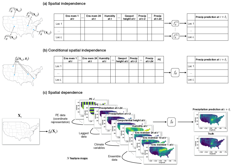
Figure 1: An illustration of different forecasting paradigms: (a) spatial independence models with a model for each spatial location, no accounting for spatial information; (b) conditional spatial independence models with one model for all locations, might consider the spatial information; (c) spatial dependence models that account for the spatial information by the design. For temperature prediction, we replace “precipitation” in the illustration with “temperature”, but the overall structure remains the same.

3.3 Forecast tasks

The learning task can be formulated as learning a model $f_{\theta}:\mathbf{X}\to\mathbf{y}$ with parameters $\bm{\theta}$. This model $f_{\theta}$ can be a linear regression (where $\bm{\theta}$ is a set of regression weights), the mean of ensemble members (no $\bm{\theta}$ needs to be learned), a random forest (where $\bm{\theta}$ parameterizes the set of trees in the forest), a convolutional neural network (where $\bm{\theta}$ are the neural network weights), or other learned models. We consider three different forecasting tasks: regression, tercile classification, and quantile regression.

Regression

The goal of regression is to predict monthly average values of precipitation and 2-meter temperature two weeks in the future. These models are generally trained using the squared error loss function:

$$\ell_{\rm sq-err}(\theta)=\mathbb{E}[(y-f_{\theta}(\mathbf{x}))^{2}].$$

Tercile classification

The goal of tercile classification is to predict whether the precipitation or 2-meter temperature will be “high” (above the $66$th percentile, denoted $q=1$), “medium” (between the $33$rd and the $66$th percentiles, denoted $q=0$), or “low” (below the $33$rd percentile, denoted $q=-1$). We compute these percentile values using 1971-2000 data from the NOAA dataset (see Section 4 for details), and these percentiles are computed for each calendar month $m$ and location $l$ pair. These models are generally trained using the cross-entropy loss function:

$$\ell_{\rm CE}(\theta)=\mathbb{E}\left[\sum_{q=-1}^{1}-{{\mathbb{I}_{\{y=q\}}}}\log(f_{\theta}(\mathbf{x}))_{q}\right],$$

where ${{\mathbb{I}_{\{A\}}}}:={\begin{cases}1,&\text{if }A\text{ true}\\ 0,&\text{if }A\text{ false}\end{cases}}$ is the indicator function and $(f_{\theta}(x))_{q}$ is the predicted probability that the target $y$ corresponding to feature vector $x$ will be in tercile $q$.

Quantile regression

For a given percentile $\alpha$, the goal of quantile regression is to predict the value $z$ so that, conditioned on features $x$, the target $y$ satisfies $y\leq z$ with probability $\alpha$. When we set $\alpha$ to a value close to one, such as $\alpha=0.9$, this value $z$ indicates what we can expect in “extreme outcomes”, not just on average. These models are generally trained using the pinball loss function:

$$\ell_{\rm quantile}(\theta)=\mathbb{E}[\rho_{\alpha}(y-f_{\theta}(\mathbf{x}))]\\$$ (1)

where

$$\rho_{\alpha}(z):=z(\alpha-{{\mathbb{I}_{\{(z<0)\}}}})=\begin{cases}\alpha|z|&\text{if }z\geq 0\\ (1-\alpha)|z|&\text{if }z<0\end{cases}.$$ (2)

4 Data

Table 1 presents a description of variables that are used in the experiments. Historical averages of precipitation and temperature (or “climatology”) are calculated using 1971-2000 NOAA data [30]. There are many ensembles of physics-based predictions produced by forecasting systems. NMME provides forecasts from multiple global forecast models from North American modeling centers [10]. The NMME project has two predictive periods: hindcast and forecast. A hindcast period refers to when a dynamic model re-forecasts historical events, which can help climate scientists develop and test new models to improve forecasting as well as to evaluate model biases. In contrast, a forecast period has real-time predictions generated from dynamic models.

Table 1: Description of climate variables and their data sources. Our target climate variables for sub-seasonal climate forecasting are precipitation and 2-meter temperature. Since ground truth observations span a relatively short period of time, we use NOAA data to calculate historical averages from 1971 to 2000. We also perform linear spatial interpolation on the historical values to get values with the same support as target climate variables.

Type	Variable	Description	Unit	Spatial Coverage	Time Range	Data Source
Climate variable	tmp2m	Daily average temperature at 2 meters	${}^{\circ}C$	US mainland $0.5^{\circ}\times 0.5^{\circ}$ grid	1985 to 2020	CPC Global Daily Temperature [31]
	precip	Daily average precipitation	mm	US mainland $0.5^{\circ}\times 0.5^{\circ}$ grid	1985 to 2020	CPC Global Daily Precipitation [32]
	SSTs	Daily sea surface temperature	${}^{\circ}C$	Ocean only $0.25^{\circ}\times 0.25^{\circ}$ grid	1985 to 2020	Optimum Interpolation SSTs High Resolution (OISST) [33]
	rhum	Daily relative humidity near the surface	Pa
	slp	Daily pressure at sea level	$\%$	US mainland and North Pacific & Atlantic Ocean $0.5^{\circ}\times 0.5^{\circ}$ grid	1985 to 2020	Atmospheric Research Reanalysis Dataset [34]
	hgt500	Daily geopotential height at 500mb	m
Historical	tmp2m	Daily average temperature at 2 meters	K	Globally $1^{\circ}\times 1^{\circ}$ grid	1971 to 2000	NOAA [30]
	precip	Daily average precipitation	mm	Globally $1^{\circ}\times 1^{\circ}$ grid	1971 to 2000	NOAA [30]

In this manuscript, we use ensemble forecasts from the NMME’s NCEP-Climate Forecast System version 2 (CFSv2, Kirtman et al. [10], Saha et al. [11]), which has $K=24$ ensemble members at a $1^{\circ}\times 1^{\circ}$ resolution over a 2-week lead time. NCEP-CFSv2 is the operational prediction model currently used by the U.S. Climate Prediction Center. The NCEP-CFSv2 model has two different products: we use its hindcasts from 1982 to 2010 for training and validation of our models, and we use its forecasts from April 2011 to December 2020 for final evaluation of our models.

In order to ensure our results are not unique to a single forecasting model, we also analyze output from the NASA-Global Modeling and Assimilation (GMAO) from the Goddard Earth Observing System model version 5 (GEOS, Nakada et al. [12]), which has $K=11$ ensemble members at a $1^{\circ}\times 1^{\circ}$ resolution over a 2-week lead time. Similarly, we use its hindcasts from 1981 to 2010 for training and validation of our models, and we use its forecasts from January 2011 to January 2018 for final evaluation. The test periods of NCEP-CFSv2 and NASA-GMAO data are different due to the data availability.

Different ensemble members correspond to different initial conditions of the underlying physical model. The NCEP-CFSv2 forecasts are initialized in the following way: four initializations at times 0000, 0600, 1200, and 1800 UTC every fifth day, starting one month prior to the lead time of two weeks (Table B1 in Saha et al. [11]). NASA-GMAO is a fully coupled atmosphere–ocean–land–sea ice model, with forecasts initialized every five days.

All data are interpolated to lie on the same $1^{\circ}\times 1^{\circ}$ grid, resulting in $L=3,274$ U.S. locations. Climate variables that are available daily (such as pressure at sea level or precipitation) are converted to monthly average values. When data are available as monthly averages only, we ensure that our forecast for time $t+\delta_{t}$ does not use any information from the interval $(t,t+\delta_{t})$.

5 Prediction methods

5.1 Baselines

Climatology (i.e., historical average)

This simple baseline is the 30-year mean of a variable at a given location and month. It is the fundamental benchmark for climate predictability. In particular, for a given time $t$, let $m(t):=(t\mod 12)$ correspond to the calendar month corresponding to $t$; then we compute the 30-year climatology of the target variable for a given location and time via

$$\hat{y}_{t,l}^{\rm hist}=s_{m(t),l},\leavevmode\nobreak\ t=1,\dots,T,\leavevmode\nobreak\ l=1,\dots,L.$$ (3)

Ensemble average

This is the mean of all ensemble members for each location $l$ at each time step $t$:

$$\hat{y}_{t,l}^{\rm ens\leavevmode\nobreak\ avg}:=\frac{1}{K}\sum_{k=1}^{K}u_{t,l}^{(k)},\leavevmode\nobreak\ t=1,\dots,T,\leavevmode\nobreak\ l=1,\dots,L.$$ (4)

Linear regression

Finally, we consider a baseline of a linear regression model applied to input features corresponding to ensemble member predictions: $\mathbf{x}_{t,l}=[u^{(1)}_{t,l},\dots,u^{(K)}_{t,l}]$. Then the model’s output

$$\hat{y}_{t,l}^{\rm LR}:=\langle\bm{\theta}_{l},\mathbf{x}_{t,l}\rangle+\theta_{l}^{0},$$ (5)

where $\theta_{l}$ are the trained coefficients for input features for each location $l$, and $\theta_{l}^{0}$ are the learned intercepts for each location $l$. Note that we train a different model for each spatial location, and the illustration for this model and its input’s format is given in Figure 1(a).

5.2 Learning-based methods

Linear regression (LR)

In contrast to the linear regression baseline, here other climate variables are added to the input features: $\mathbf{x}_{t,l}=[u^{(1)}_{t,l},...,u^{(K)}_{t,l},v^{(1)}_{t,l},...,v^{(P)}_{t,l}]$. Then the model’s output is defined with Eq. 5 . Because the feature vector is higher dimensional here than for the baseline, the learned $\theta_{l}$ is also higher dimensional. We train a different model for each spatial location. In our experiments with linear models, we do not include positional encoding $(\mathbf{z}_{l}^{(1)},\mathbf{z}_{l}^{(2)})$ as input features, since they would be constants for that location’s linear model.

In the context of regression, we minimize the squared error loss. The linear quantile regressor (Linear QR) is a linear model trained to minimize the quantile loss

$$\ell^{\rm QR}=\frac{1}{L}\sum_{l=1}^{L}\left[\frac{1}{T}\sum_{t=1}^{T}\rho_{\tau}\left(y_{t,l}-\hat{y}_{t,l,}\right)\right],$$ (6)

where $\rho_{\tau}$ is defined in Eq. 2.

Random forest

In the context of regression and tercile classification, we train a random forests that use ensemble predictions, the spatial location, and additional climate features to form the feature vector $\mathbf{x}_{t,l}=[u^{(1)}_{t,l},...,u^{(K)}_{t,l},v^{(1)}_{t,l},...,v^{(P)}_{t,l},\mathbf{z}_{l}^{(1)},\mathbf{z}_{l}^{(2)}]$ for all location $l$ and time $t$ pairs. One random forest is trained to make predictions for any spatial location. The illustration for RF and its input’s format is given in Figure 1(b): we train one RF model for all locations, and the spatial information is encoded as input features via PE vectors $\mathbf{z}_{l}^{(1)},\mathbf{z}_{l}^{(2)}$.

In the context of quantile regression, we train a random forest quantile regressor (RFQR, [35]), which grows trees the same way as the original random forest while storing all training samples. To make a prediction for a test point, the RFQR computes a weight for each training sample that corresponds to the number of leafs (across all trees in the forest) that contain the test sample and the training sample. The RFQR prediction is then a quantile of the weighted training samples across all leafs that contain the test sample. We show a figure representation of the RFQR in Section D. With this formulation, training a single RFQR for all locations is computationally demanding, so we train individual RFQRs for every location.

The RFs are often referred as the best off-the-shelf classifiers [36] even using the default hyperparameters [37]. Our cross-validation (CV) and grid search experiments show that the RFs hyperparameters have little impact on the accuracy. So, we use the default parameters for RFs from the Scikit-learn library [38].

Convolutional neural network

To produce a forecast map for the U.S., we adapted a U-Net architecture [39], which has an encoder-decoder structure with convolutional layer blocks. The U-Net maps a stack of images to an output image; in our context, we treat each spatial map of a climate variable or forecast as an image. Thus, the input to our U-Net is can be represented as a tensor composed from matrices: $\mathbf{X}_{t}=[\mathbf{U}^{(1)}_{t},...,\mathbf{U}^{(K)}_{t},\mathbf{V}^{(1)}_{t},...,\mathbf{V}^{(P)}_{t},\mathbf{Z}^{(1)},\mathbf{Z}^{(2)}]$.

Note that here we use capital letters because the input to our U-Net consists 2-D spatial maps, which are represented as matrices instead of vectors. The model output is a spatial map of the predicted target. This process is illustrated in Figure 1(c).

For the U-Net, we modify an available PyTorch implementation [40]. We use 10-fold CV over our training data and grid search to select parameters such as learning rate, weight decay, batch size, and number of epochs. The Adam optimizer [41] is used in all experiments. After selecting hyperparameters, we train the U-Net model with those parameters on the full training dataset. The validation set is used to perform feature importance analysis. For regression, we train using squared error loss. In the context of quantile regression, we initialize the weights with those learned on squared error loss and then train on the quantile loss Eq. 6.

Nonlinear model stacking

Model stacking can improve model performance by combining the outputs of several models (usually called base models) [42]. In our case, linear regression, random forests, and the U-Net are substantially different in terms of architecture and computation, and we observe that they produce qualitatively different forecasts. We stack a linear model, random forest, and U-Net using a nonparametric approach:

$$\hat{y}_{t,l}=h(\hat{y}_{t,l}^{\text{LR}},\hat{y}_{t,l}^{\text{RF}},\hat{y}_{t,l}^{\text{UNET}}),$$ (7)

where $h$ is a simple feed-forward neural network with a non-linear activation, $\hat{y}_{t,l}^{\text{LR}},\hat{y}_{t,l}^{\text{RF}},\hat{y}_{t,l}^{\text{UNET}}$ are the predictions of a linear model, random forest and the U-Net correspondingly and referred to as ”base models”. One stacking model is trained to make predictions for any spatial location. Figure 1(b) demonstrates the stacking model’s input format and framework: the features are predictions from other ML models, and there is no spatial information. Model stacking can improve the forecast quality by combining predictions from three forecasting paradigms – spatial independence, conditional spatial independence, and spatial dependence (Section 3.2). The architecture details can be found in Appendix D.

For model stacking, we apply the following procedure: the base models are first trained on half of the training data, and predicted values on the second half are used to train the stacking model $h$. Then we retrain the base models on all the training data and apply the trained stacked model to the outputs of the base models. The proposed procedure helps avoid overfitting.

6 Experimental setup

In this section, we provide details on the experimental setup including positional encoding, removing climatology, and evaluation metrics. Data preprocessing details are presented in Appendix E.

6.1 Subtracting climatology

We evaluate our detrended predictions against the detrended true responses, defined as

$$y_{t,l}^{\text{detrended}} =y_{t,l}-s_{m(t),l},$$ (8)

$$\hat{y}_{t,l}^{\text{detrended}} =\hat{y}_{t,l}-s_{m(t),l},$$ (9)

where $s_{m,l}$ is defined in Eq. (3). However, for the special case of $\hat{y}$ corresponding to the ensemble average, the ensemble members may exhibit bias, in which case we also consider

$$\hat{y}_{t,l}^{\text{detrended}} =\hat{y}_{t,l}-\hat{s}_{m(t),l},$$ (10)

where $\hat{s}_{m(t),l}$ is evaluated on the model’s (ensemble average) predictions:

$$\hat{s}_{m,l}:=\frac{1}{T}\sum_{t=1}^{T}\hat{y}_{t,l}{{\mathbb{I}_{\{m=m(t)\}}}},\leavevmode\nobreak\ l=1,\dots,L.$$ (11)

The model climatology $\hat{s}_{m,l}$ is computed using the training data. Note that we do not apply detrending to the input features and target variables, i.e., precipitation and temperature when training our ML models. We subtract climatology from the model outputs only when evaluating their performance.

6.2 Positional encoding and inputs

Positional encoding [43] is a technique used in natural language processing (NLP) to inject positional information into data. In sequence-based tasks, such as language translation or text generation, the order of elements in the input sequence is important, but neural networks do not naturally capture this information. PE assigns unique encodings to each position in the sequence, which are then added to the original input before being processed by the model. This enables the model to consider the order and relative positions of elements, improving its ability to capture local and global context within a sequence and make accurate predictions [44, 45, 46]. This technique is helpful to represent the positional information outside of the NLP tasks [47, 48, 49]. Several of our models use the spatial location as an input feature. Rather than directly using latitudes and longitudes, we use PE [43]:

$$z_{l}^{(1)}(i)= {\operatorname{PE}}(l,2i)=\sin(l/10000^{2i/d}),$$ (12)

$$z_{l}^{(2)}(i)= {\operatorname{PE}}(l,2i+1)=\cos(l/10000^{2i/d}),$$ (13)

where $l$ is a longitude or latitude value, $d=12$ is the dimensionality of the positional encoding, and $i\in\{1,\dots,d\}$ is the index of the positional encoding vector. For the U-Net model, PE vectors are transformed into images in the following way: we take every value in the vector and fill the image of desired size with this value. So, there are $d$ images with the corresponding PE values. For the RF models, PE vectors can be used as they are.

To summarize, as input features to our ML models, we use

• $K$ ensemble forecasts for the target month,

• four climate variables such as relative humidity, pressure, geopotential height, and temperature (if target is precipitaion) or precipitation (if target is temperature) two months before the target month,

• the lagged target variable (the target variable two, three, four, twelve and 24 months before the target date – five additional features),

• SSTs that are represented via principal components (PCs),

• and, finally, the positional embeddings.

SSTs are usually represented as eights PCs, the embedding vector size is usually $d=12$ as we describe Section 6.2. For example, using the NCEP-CFSv2 members, there are $\underbrace{24}_{K}+\underbrace{4+5+8}_{P}+\underbrace{12}_{d}*2=65$ input features for every time step and location.

6.3 Evaluation metrics

Regression metrics

The forecast skill of our regression models is measured using the $R^{2}$ value. For each location $l$ and ground-truth values $y_{t,l}$ and predictions $\hat{y}_{t,l}$ at this location, we compute

$$R^{2}_{l}=1-\frac{{\sum_{t=1}^{T}}(y_{t,l}^{\text{detrended}}-\hat{y}_{t,l}^{\text{detrended}})^{2}}{{\sum_{t=1}^{T}}(y_{t,l}^{\text{detrended}}-\bar{y}_{l}^{\text{detrended}})^{2}},$$ (14)

where

$$\bar{y}_{l}^{\text{detrended}}=\frac{1}{T}\sum_{t=1}^{T}\hat{y}_{t,l}^{\text{detrended}}.$$

Then the average $R^{2}$ for all locations is calculated as

$$R^{2}=\frac{1}{L}\sum_{l=1}^{L}R_{l}^{2}.$$ (15)

In addition to the average $R^{2}$ on the test data, we also estimate the median $R^{2}$ score across all U.S. locations.

We further report the mean squared error (MSE) of our predictions across all locations:

$${\rm MSE}_{l}:=\frac{1}{T}\sum_{t=1}^{T}\left(y_{t,l}-\hat{y}_{t,l}\right)^{2},$$

for $l=1,\dots,L$, and

$${\rm MSE}=\frac{1}{L}\sum_{l=1}^{L}{\rm MSE}_{l}.$$ (16)

We also report the standard error (SE), median, and 90th percentile of $\{{\rm MSE}_{l}\}_{l}$. (We say that the difference between two models is significant if their MSE $\pm$ SE intervals do not overlap. However, the standard errors provided here should be used with caution since there are significant spatial correlations in the MSE values across locations, so we do not truly have $L$ independent samples from an asymptotically normal distribution.)

Tercile classification metrics

We estimate the accuracy of our tercile classification predictions as the proportion of correctly classified samples out of all observations.

Quantile regression metrics

For the quantile regression task, we report mean quantile loss (6) across all locations.

7 Experimental results

In this section, we report the predictive skill of different models applied to SSF over the continental U.S.  using NCEP-CFSv2 ensemble members for regression and quantile regression. Precipitation forecasting is known to be more challenging compared to temperature forecasting [50]. The results for the NASA-GMAO dataset are presented in Supplemental Material A. The skill of different models on the tercile classification task is presented in Supplemental Material B for both datasets. Recall that all methods are trained on data spanning January 1985 - October 2005, with data spanning November 2005 - December 2010 used for validation (i.e., model selection and hyperparameter tuning). Test data spanning 2011 to 2020 was not viewed at any point of the model development and training process, and only used to evaluate the predictive skill of our trained models on previously unseen data; we refer to this period as the “test period”. The code is available at https://github.com/elena-orlova/SSF-project. As a navigation tool for the reader, Table 2 gives references to the presented results for different tasks.

Table 2: A table with references to the main results.

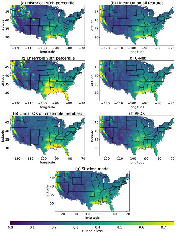
Figure 14: Test quantile loss heatmaps of baselines and learning-based methods for precipitation quantile regression using NASA-GMAO dataset. Blue regions indicate smaller quantile loss. See Section A.2 for details.

Task	Data	Reference
Regression	precip NCEP-CFSv2	Table 3; Figure 2
	tmp NCEP-CFSv2	Table 4; Figure 3
	precip NASA-GMAO	Table 12; Figure 12
	tmp NASA-GMAO	Table 13; Figure 13
Quantile regression	precip NCEP-CFSv2	Table 5; Figure 4
	tmp NCEP-CFSv2	Table 6; Figure 5
	precip NASA-GMAO	Table 14; Figure 14
	tmp NASA-GMAO	Table 15; Figure 15
Feature importance	precip NCEP-CFSv2	Table 9
	tmp NCEP-CFSv2	Table 10
Tercile classification	precip NCEP-CFSv2	Table 16; Figure 16
	tmp NCEP-CFSv2	Table 17; Figure 18
	precip NASA-GMAO	Table 16; Figure 17
	tmp NASA-GMAO	Table 17; Figure 19

7.1 Regression

Precipitation regression

Precipitation regression results are presented in Table 3. Our methods, especially the stacked model, frequently outperform the MSE of baselines, such as the ensemble average or historical average significantly. In addition, the mean and median $R^{2}$ values of the stacked model are the highest compared to all other methods. Note that the best $R^{2}$ value, associated with the stacked model, is still near zero; while this is a significant improvement over, for example, the ensemble average, which has an $R^{2}$ value of -0.08, the low values for all methods indicate the difficulty of the forecasting problem. It is important to note that $R^{2}$ measures the accuracy of a model relative to a baseline corresponding to the mean of the target over the test period – that is, relative to a model that could never be used in practice as a forecaster because it uses future observations. The best practical analog to this would be the mean of the target over the train period – what we call the “historical average” model. These two models are not the same because of the nonstationarity of the climate. Thus even when our $R^{2}$ values are negative (i.e., we perform worse than the impractical mean of the target over the test period), we still perform much better than the practical historical average predictor. The model stacking approach is applied to the models that are trained on all available features (i.e., ensemble members, positional encoding, lagged data, climate variables; linear regression is trained on all features except PE). We decide what models to include in the stacking approach based on their performance on validation data. The low 90th percentile error implies that our methods not only have high skill on average, but also that there are relatively few locations with large errors. While acknowledging the overall performance may not be exceptional, it is important to recognize the potential of machine learning methods in improving the quality of estimates relative to standard baselines.

Table 3: Results for precipitation regression the using NCEP-CFSv2 ensemble, with errors reported over the test period. LR refers to linear regression on all features including ensemble members, lagged data, climate variables and SSTs. Model stacking is performed on models that are trained on all features. The best results are in bold. MSE is reported in mm.

Model	Features	Mean $R^{2}$ ($\uparrow$)	Median $R^{2}$ ($\uparrow$)	Mean Sq Err ($\downarrow$)	Median MSE ($\downarrow$)	90th prctl MSE ($\downarrow$)
	Historical avg	-0.06	-0.01	2.33 $\pm$ 0.04	1.59	4.96
	Ens avg	-0.08	0.01	2.19 $\pm$ 0.04	1.55	4.57
Baseline	Linear Regr	-0.11	-0.07	2.26 $\pm$ 0.04	1.54	4.72
LR	All features	-0.33	-0.25	2.71 $\pm$ 0.05	1.91	5.45
U-Net	All features	-0.10	-0.01	2.18 $\pm$ 0.03	1.44	4.62
RF	All features	-0.11	-0.01	2.17 $\pm$ 0.05	1.48	4.45
Stacked	LR, U-Net, RF outputs	0.02	0.04	2.07 $\pm$ 0.03	1.42	4.38

Figure 2 illustrates performance of key methods with $R^{2}$ heatmaps over the U.S. to highlight spatial variation in errors. The RF and U-Net $R^{2}$ fields are qualitatively similar, but they are still quite different in certain states such as Georgia, North Carolina, Virginia, Utah, and Colorado. The LR map is noticeably poor across most of the regions. The stacked model’s heatmap reveals large regions where its predictive skill exceeds that of all other methods. Note that model stacking yields relatively accurate predictions even in regions where the three constituent models individually perform poorly (e.g., southwestern Arizona), highlighting the generalization abilities of our stacking approach. All methods tend to have higher accuracy on the Pacific Coast, in Midwest, and in southern states such as Alabama and Missouri.

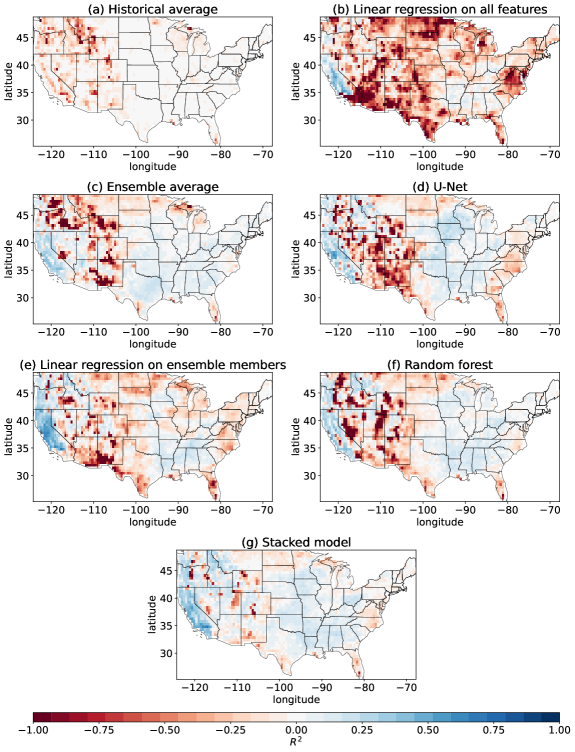
Figure 2: $R^{2}$ score heatmaps of baselines and learning-based methods for precipitation regression using NCEP-CFSv2 ensemble members; errors are computed over the test period. Positive values (blue) indicate better performance. See Section 7.1 for details.

Temperature regression

Table 4 shows results for 2-meter temperature regression. The learning-based models, especially the random forest and stacked model, significantly outperform the baseline models in terms of MSE and $R^{2}$ score. The random forest also outperforms linear regression and the U-Net. Note that LR, U-Net, and RF are trained without using SSTs information, since SSTs features yielded worse performance over the validation period. Figure 3 illustrates the performance of these methods with $R^{2}$ heatmaps over the U.S. As expected, the model stacking approach shows the best results across spatial locations. We notice that there are still regions such as the West, some regions in Texas, Florida and Georgia where all models tend to achieve a negative $R^{2}$ score.

Table 4: Results for temperature regression using the NCEP-CFSv2 ensemble, with errors reported over the test period. LR refers to linear regression on all features including ensemble members, lagged data, land variables. Model stacking is performed on models that are trained on all features except SSTs. The best results are in bold. MSE is reported in ${}^{\circ}C$.

Model	Features	Mean $R^{2}$ ($\uparrow$)	Median $R^{2}$ ($\uparrow$)	Mean Sq Err ($\downarrow$)	Median MSE ($\downarrow$)	90th prctl MSE ($\downarrow$)
	Historical avg	-0.66	-0.17	6.57 $\pm$ 0.11	5.04	9.99
	Ens avg	-0.47	0.08	5.51 $\pm$ 0.10	3.83	9.16
Baseline	Linear Regr	0.04	0.17	3.60 $\pm$ 0.03	3.25	5.49
LR	All features w/o SSTs	0.05	0.16	3.57 $\pm$ 0.02	3.33	5.41
U-Net	All features w/o SSTs	0.01	0.18	3.65 $\pm$ 0.02	3.38	5.31
RF	All features w/o SSTs	0.16	0.25	3.17 $\pm$ 0.02	2.99	4.63
Stacked	LR, U-Net, RF outputs	0.18	0.27	3.11 $\pm$ 0.02	2.93	4.56

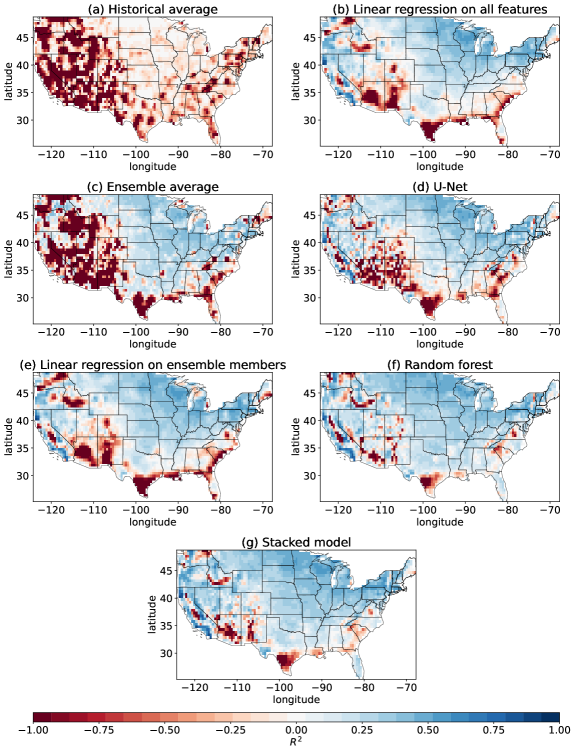
Figure 3: $R^{2}$ score heatmaps of baselines and learning-based methods for temperature regression using NCEP-CFSv2 ensemble members; errors are computed over the test period. Positive values (blue) indicate better performance. See Section 7.1 for details.

7.2 Quantile regression

We explore the use of quantile regression to predict values $z$ so that “there’s a 90% chance that the average temperature will be below $z^{\circ}$ at your location next month” – or, equivalently, “there is a 10% chance that the average temperature will exceed $z^{\circ}$ at your location next month.” In this sense, quantile regression focused on the $90$-th percentile predicts temperature and precipitation extremes, a task highly relevant to a myriad of stakeholders. We train a linear regression model fitting the quantile loss (Linear QR), a random forest quantile regressor (RFQR), [35], a U-Net, and the stacked model. Details of the Linear QR and the RFQR are discussed in Section 5. The below experimental results show that temperature extremes can be predicted with high accuracy by the learning-based models (particularly our stacked model), in stark contrast to historical quantiles or ensemble quantiles in the case of temperature quantile regression. The results for precipitation are less striking overall, though the learned models are significantly more predictive in some locations as for the precipitation quantile regression task.

Quantile regression of precipitation

For each location, the 90th percentile value is calculated based on the historical data. For the ensemble 90th percentile, we simply take the 90th percentile of the $K$ ensemble members. Table 5 summarizes results for precipitation quantile regression using the NCEP-CFSv2 ensemble. Our stacked model is able to significantly outperform all baselines. In Figure 4, we show heatmaps of quantile loss of all locations in the U.S., where blue means smaller quantile loss and yellow means larger quantile loss. We observe that the learning-based models are outperforming the baselines, especially in Washington, California, Idaho, and near the Gulf of Mexico.

Table 5: Test results for precipitation quantile regression using NCEP-CFSv2 dataset, with target quantile = 0.9. Linear QR refers to a linear quantile regressor. RFQR corresponds to a Random Forest Quantile Regressor. Model stacking is performed on models that are trained on all features. The best results are in bold. Quantile loss is reported in mm.

Model	Features	Mean Qtr Loss ($\downarrow$)	Median Qtr Loss ($\downarrow$)	90th prctl Qtr Loss ($\downarrow$)
	Historical 90th percentile	0.304 $\pm$ 0.003	0.278	0.504
	Ens 90th percentile	0.311 $\pm$ 0.003	0.275	0.488
Baseline	Linear QR ens only	0.310 $\pm$ 0.003	0.266	0.505
Linear QR	All features	0.287 $\pm$ 0.003	0.248	0.463
U-Net	All features	0.312 $\pm$ 0.002	0.281	0.504
RFQR	All features	0.282 $\pm$ 0.002	0.257	0.453
Stacked	U-Net, RFQR, LQR outputs	0.282 $\pm$ 0.002	0.256	0.457

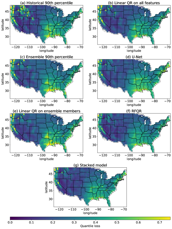
Figure 4: Test quantile loss heatmaps of baselines and learning-based methods for precipitation quantile regression using NCEP-CFSv2 dataset. Blue regions indicate smaller quantile loss. See Section 7.2 for details.

Quantile regression of temperature

Table 6 summarizes results for temperature quantile regression using the NCEP-CFSv2 ensemble. Note that we do not include SSTs features for temperature quantile regression in our learned models. We observe that all of our learned models are able to significantly outperform all baselines. In Figure 5, we show the heatmaps of quantile loss of baselines and our learned models. We observe that the learned models produce different quality predictions, and the stacked model is able to pick up useful information from them. For example, in Arizona and Texas, the Linear QR, U-Net, and RFQR show some errors but in different locations, and the stacked model is able to exploit the advantages of each model.

Table 6: Test results for temperature quantile regression using NCEP-CFSv2 dataset, with target quantile = 0.9. Linear QR refers to a linear quantile regressor. RFQR corresponds to a Random Forest Quantile Regressor. Model stacking is performed on models that are trained on all features except for SSTs . Learned models are able to predict highly likely temperature ranges accurately, meaning there are fewer unpredicted temperature spikes. The best results are in bold.

Model	Features	Mean Qtr Loss ($\downarrow$)	Median Qtr Loss ($\downarrow$)	90th prctl Qtr Loss ($\downarrow$)
	Historical 90th percentile	0.589 $\pm$ 0.008	0.435	0.980
	Ens 90th percentile	0.642 $\pm$ 0.009	0.468	1.196
Baseline	Linear QR ens only	0.336 $\pm$ 0.004	0.286	0.488
Linear QR	All features w/o SSTs	0.318 $\pm$ 0.002	0.301	0.407
U-Net	All features w/o SSTs	0.363 $\pm$ 0.003	0.329	0.488
RFQR	All features w/o SSTs	0.320 $\pm$ 0.002	0.307	0.384
Stacked	U-Net, RFQR, LQR outputs	0.287 $\pm$ 0.001	0.285	0.344

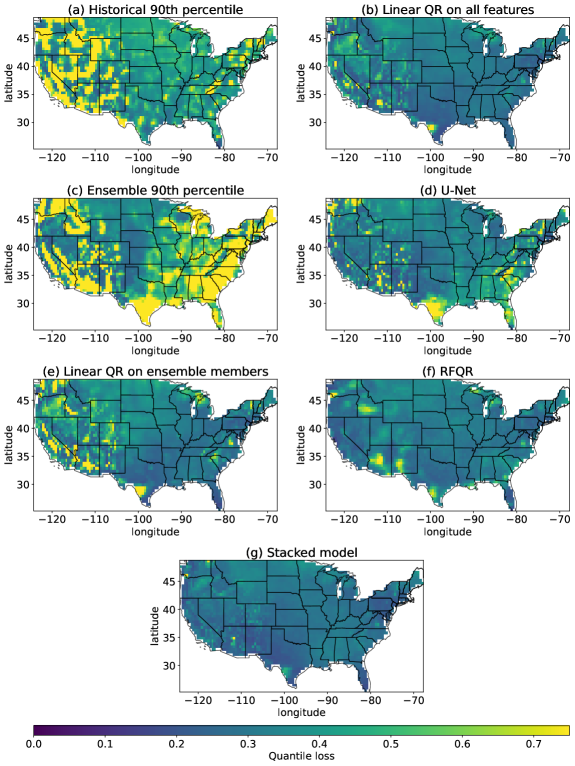
Figure 5: Test quantile loss heatmaps of baselines and learning-based methods for temperature quantile regression using NCEP-CFSv2 dataset. Blue regions indicate smaller quantile loss. See Section 7.2 for details.

8 Discussion

8.1 The efficacy of machine learning for SSF

While climate simulations and ensemble forecasts are designed to provide useful predictions of temperature and precipitation based on carefully developed physical models, we see that machine learning applied to those ensembles can yield a significantly higher predictive skill for a range of SSF tasks. Figure 6 illustrates key differences between different predictive models for predicting precipitation 14 days in advance. Individual ensemble members are predictions with high levels of spatial smoothness and more extreme values. Linear regression, the random forest, the U-Net, and the stacked model produce higher spatial frequencies. The linear regression result, which uses a different model trained for each spatial location separately, has the least spatial smoothness of all methods; this is especially visible in the southeast and potentially does not reflect realistic spatial structure. The learning-based models more accurately predict localized regions of high and low precipitation compared to the ensemble average.

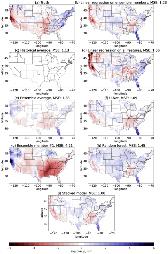
Figure 6: An illustration of precipitation predictions (on the detrended scale in mm) of different methods for February 2016 (in test period). (a) True precipitation. (b) LR on ensemble members. (c) Historical average. (d) LR on all features. (e) Ensemble average. (f) U-Net on all features. (g) Example single ensemble member. (h) Random forest on all features. (i) Stacked model. See Section 8.1 for details.

Figure 7 demonstrates differences between the ground truth and different model predictions. In this figure, the color white is associated with the smallest errors, while red pixels indicate overestimating precipitation and blue pixels indicate underestimating precipitation. The individual ensemble member in Figure 7(e) exhibits dark red regions across the West, while the ensemble average in Figure 7(e) shows better performance in this area. The colors are more muted for the stacked model in Figure 7(h). The historical average in Figure 7(a) has the most neutral areas. However, its MSE is slightly higher than the stacked model’s MSE. In general, all methods, including linear regression (b, d), U-Net (f) and random forest (g), tend to underpredict precipitation in the Southeast, Mid-Atlantic and North Atlantic and predict higher precipitation levels in the West. Several hypotheses might explain why ML is an effective approach for SSF, and we probe those hypotheses in this section.

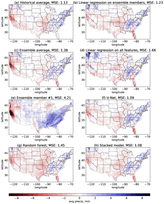
Figure 7: An illustration of differences $y_{t,l}^{\text{detrended}}-\hat{y}_{t,l}^{\text{detrended}}$ in precipitation predictions in mm of different methods for February 2016 (in test period). Red pixels indicate areas where a forecasting method predicts higher precipitation levels compared to the ground truth, blue pixels indicate an underestimation of the precipitation, and white pixels correspond to a precise prediction. See Section 8.1 for details.

Using full ensemble vs. ensemble average

Past works use ensemble average as an input feature to machine learning methods in addition to the climate variables [8, 27]. Ensembles provide valuable information not only about expected climate behavior but also variance or uncertainty in multiple dimensions; methods that rely solely on ensemble average lack information about this variance. The dynamical models that underpin each ensemble member may have systematic errors, either in the mean, the variability, or conditioned upon certain elements of the initial conditions that are not readily apparent to the forecast model. While taking the average of these ensemble members may net out the deficiencies of each individual member, it is also possible that the systematic errors of each may be directly discovered and corrected by a machine learning model independently. Therefore, using a single ensemble statistic, such as the ensemble mean, as a feature may not fully capitalize on the information provided by using all the ensemble forecasts as features. In our experiments, we find that using all available ensemble members enhances the prediction quality of our approaches. As an illustration, we show the results of the stacked model using LR, RF, and U-Net trained on all ensemble members, compared to the ML models trained on the ensemble average and the sorted ensemble. In addition to the full ensemble or the ensemble mean, we use other available features (as in our previous regression results). Table 7 and Figure 8 demonstrates the results: using all ensemble members is indeed crucial. The stacked model’s performance with the full ensemble (and other features) is significantly better than its performance with just the ensemble mean (and other features) both in terms of MSE and $R^{2}$ value. We conclude that the full ensemble contains important information for SSF aside from the ensemble mean, and our models are able to capitalize on this information. A more detailed analysis is shown in Section C.1.

We can perform a statistical test to verify that these performance discrepancies are statistically significant. As before, let $\hat{y}_{t,l}$ refer to the estimate under our usual stacked model (i.e., with all ensemble members). Let $\hat{y}_{t,l}^{\text{SEA}}$ refer to a stacked model with just the ensemble average in place of each ensemble member. We can employ a sign test framework [51] to compare model performance under minimal distributional assumptions. Namely, we only make the following i.i.d. assumption over the time dimension:

$${{\mathbb{I}_{\{|\hat{y}_{t,l}-y_{t,l}|<|\hat{y}_{t,l}^{\text{SEA}}-y_{t,l}|\}}}}\overset{\text{iid}}{\sim}\mathrm{Bernoulli}(p_{l})$$

Intuitively, this corresponds to assuming it is a coin flip which model will perform better at each time point and location, and we would like to test whether each location’s “coin” is fair or not. We can then formulate our null and alternative hypotheses for each location $l$ as follows:

$$H_{0,l}:p_{l}=0.5,\;\;H_{0,l}:p_{l}>0.5$$

Thus, our overall test for significance is for the global null hypothesis $H_{0}=\cap_{l=1}^{3274}H_{0,l}$. Specifically, we calculate a p-value for each $H_{0,l}$, and then we check whether any of these p-values is below a Bonferroni-corrected threshold of $0.05/3274=1.53\times 10^{-5}$, where 3274 refers to the number of locations. In fact, the minimum p-values for this test with precipitation and regression alike are far below this threshold ($1.68\times 10^{-10}$ and $4.42\times 10^{-24}$, respectively). This allows us to reject the global null hypothesis for both temperature and precipitation, and we conclude that including the full ensemble in our stacked model significantly outperforms including just the ensemble average.

Table 7: Performance comparison of stacked model of LR, RF, and U-Net trained using the ensemble average, using the sorted ensemble members or using the full ensemble, in addition to other features. Scores on the test data are reported and NCEP-CFSv2 data is used. The best results are in bold. MSE is reported in mm for precipitation and in ${}^{\circ}C$ for temperature.

Target	Features	Mean $R^{2}$ ($\uparrow$)	Mean Sq Err ($\downarrow$)
	Ensemble avg + all features	-0.08	2.28 $\pm$0.04
Precip	Sorted ensemble + all features	-0.11	2.24$\pm$0.04
	Full ensemble + all features	0.02	2.07$\pm$ 0.04
	Ensemble avg + all features wo SSTs	0.11	3.35 $\pm$0.02
Tmp	Sorted ensemble + all features wo SSTs	0.03	3.70 $\pm$0.02
	Full ensemble + all features wo SSTs	0.18	3.11$\pm$0.02

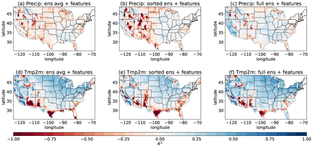
Figure 8: Test $R^{2}$ heatmaps of the stacked model of LR, RF, and U-Net trained using the ensemble average, using the sorted ensemble members or using the full ensemble, in addition to other features. The NCEP-CFSv2 ensemble is used. See Section 8.1 for details.

Learning when to trust each ensemble member

We consider the hypothesis that there is a set of $k$ ensemble members that are always best. To test this hypothesis, we use a training period to identify which $k$ members perform best for each location, and then during the test period, compute the average of only these $k$ ensemble members. The performance of this approach depends on $k$, the number of ensemble members we allow to be designated “good,” but the performance for any $k$ never exhibited a significant improvement over the ensemble average.

If the ensemble members have different levels of accuracy over various seasons, locations, and conditions, then a machine learning model may be learning when to “trust” each member. We conduct an experiment designed to test whether it is important to keep track of which ensemble member made each prediction or whether it is the distribution of predictions that is important. The modeling approach for the former would be to feed in ensemble member 1’s forecast as the first feature, ensemble member 2’s forecast as the second feature, etc. The modeling approach under the distributional hypothesis is to make the smallest prediction be the first feature, the second-smallest prediction be the second feature, and so on – i.e., we sort the ensemble forecasts for each location separately. Note that this entails treating the ensemble members symmetrically: the model would give the same prediction if ensemble member 1 predicted $a$ and ensemble member 2 predicted $b$ or if ensemble member 1 predicted $b$ and ensemble member 2 predicted $a$. In statistical parlance, this is passing in the order statistics of the forecasts as the features, rather than their original ordering. (Note that for NCEP-CFSv2, ensemble forecasts are originally ordered according to the time at which their initial conditions are set [11].) We train and evaluate the stacked model with the sorted forecasts as the features and compare to our earlier results, which used the original ordering of the ensemble members. Table 7 and Fig. 8 illustrates results over the test period. In the case of precipitation, the MSE of the sorted approach is 2.24, which is worse than the 2.07 MSE for using the original ordering. In the case of temperature forecasting, the MSE of the sorted approach is 3.70, which is much worse than the 3.11 MSE for using the original ordering. The mean $R^{2}$ of the sorted approach is also lower compared to the original ordering. In both cases, the performance is better when we feed in the features in such a way that the machine learning model has an opportunity to learn aspects of each ensemble member, not merely their order statistics. Therefore, imposing a symmetric treatment of ensemble members degrades performance. We also report results for the LR, RF, and U-Net with sorted ensemble comparing with original ordering in Appendix C.1.

8.2 Using spatial data

There are a few ways to incorporate information about location in our models. U-Net has access to the spatial dependencies by its design. Specifically, our U-Net inputs the spatial location of each point in the map. Naively, we might represent each location using the latitude and longitude values. Alternatively, we may use positional encoding, which is known to be beneficial in many ML areas, not only in NLP (as we mention in Section 66.2). It is probably due to the way PE is designed: it captures the order (or position) and allows one to learn the contextual relationships (local context – relationships between nearby elements, and global context dependencies across the entire sequence). We assume that the PE approach represents spatial information in a manner more accessible to our learned models. As an illustration, Table 8 and Figure 9 demonstrates the performance of a stacked model using LR, RF and U-Net trained using positional encoding, using latitude and longitude values and using no features representing the spatial information (no PE and no latitude or longitude values). Other inputs to the LR, RF and U-Net models are ensemble member forecasts, lagged target variable, climate variables, and SSTs (no SSTs in the case of temperature forecasting). The results suggest that using PE enhances the predictive skill of our models, compared to using just the lat/lon values or no location information, especially for the temperature forecasting task. Using no information about locations hurts the performance for precipitation regression. Thus, our models can account for spatial dependencies using input features, and PE is more beneficial than the raw latitude and longitude information. We show a more detailed analysis with results for the LR, RF and U-Net in Section C.2.

Table 8: Test performance comparison of the stacked model of LR, RF, and U-Net trained using no spatial features, using latitude and longitude values or using PE. Utilizing spatial representations, including PE, latitude, and longitude values, helps advance the predictive skill. Furthermore, using positional encoding is more beneficial than using raw latitude and longitude values. The best results are in bold. MSE is reported in mm for precipitation and in ${}^{\circ}C$ for temperature.

Target	Features	Mean $R^{2}$ ($\uparrow$)	Mean Sq Err ($\downarrow$)
	All + no location info	-0.05	2.13$\pm$0.03
Precip	All + lat/lon values	-0.01	2.21$\pm$0.04
	All + PE	0.02	2.07$\pm$0.03
	All + no location info	0.12	3.35$\pm$0.02
Tmp	All + lat/lon values	0.12	3.33$\pm$0.02
	All + PE	0.18	3.11$\pm$ 0.02

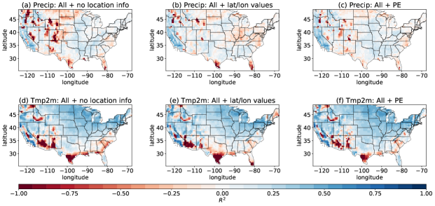
Figure 9: Test $R^{2}$ heatmaps of the stacked model of LR, RF, and U-Net trained using no spatial features, using latitude and longitude values or using PE. The NCEP-CFSv2 ensemble is used. See section 8.2 for details.

8.3 Variable importance

One consideration when implementing ML for SSF is that ML models can incorporate side information (such as spatial information, lagged temperature and precipitation values, and climate variables). We explore the importance of the various components of side information in this section. We see that including the observational climate variables improve the performance for both the random forest and the U-Net when doing precipitation regression. Furthermore, including positional encoding of the locations improves the performance of the U-Net, while the principle components of the sea surface temperature do not make notable difference in the case of temperature prediction.

More specifically, Table 9 summarizes grouped feature importance of precipitation regression using the NCEP-CFSv2 ensemble. We observe that models, in particular random forest and U-Net, trained on all available data achieve the best performance. In the case of linear regression, the SSTs features are neither very helpful nor actively harmful. Therefore, in order to be consistent, we use predictions of these models trained on all features as input to the stacking model.

Table 9: Grouped feature importance results on validation for precipitation regression task using NCEP-CFSv2 ensemble members. The results suggest that using additional observational information helps to improve the performance of learning-based models for this task. –"– means a repetition of features that are used above. For example, in the U-Net part of the table, “–"– & lags” means that ensemble members, PE, and lags are used as features and “–"– & SSTs” means ensemble members, PE and lags, land features and SSTs are used as features. The best results are in bold. MSE is reported in mm.

Model	Features	Mean $R^{2}$ ($\uparrow$)	Median $R^{2}$ ($\uparrow$)	Mean Sq Err ($\downarrow$)	Median MSE ($\downarrow$)	90th prctl MSE ($\downarrow$)
LR	Ens members	-0.13	-0.08	2.11 $\pm$ 0.03	1.53	4.63
	–"– & lags	-0.11	-0.07	2.10 $\pm$ 0.03	1.50	4.59
	–"– & climate variables (no SSTs)	-0.09	-0.06	2.06 $\pm$ 0.03	1.47	4.52
	–"– & SSTs	-0.10	-0.07	2.08 $\pm$ 0.03	1.47	4.61
U-Net	Ens members with PE	-0.13	-0.05	2.01 $\pm$ 0.03	1.50	4.31
	–"– & lags	-0.08	-0.02	1.92 $\pm$ 0.03	1.42	4.17
	–"– & climate variables (no SSTs)	-0.02	0.05	1.86 $\pm$ 0.03	1.37	4.02
	–"– & SSTs	0.00	0.05	1.83 $\pm$ 0.03	1.34	3.94
RF	Ens members with PE	-0.15	-0.04	2.02 $\pm$ 0.03	1.49	4.34
	–"– & lags	-0.10	0.00	1.96 $\pm$ 0.03	1.44	4.21
	–"– & climate variables (no SSTs)	-0.08	0.02	1.93 $\pm$ 0.03	1.39	4.16
	–"– & SSTs	-0.06	0.04	1.89 $\pm$ 0.03	1.36	4.08

Table 10 summarizes grouped feature importance of temperature regression using the NCEP-CFSv2 ensemble. In this case, adding some types of side information may yield only very small improvements to predictive skill, and in some cases the additional information may decrease predictive skill. This may be a sign of overfitting. We also note that SSTs provide only marginal (if any) improvement in predictive skill, in part because Pacific SSTs are less helpful away from the western U.S [52, 53]. It could also be that information from the SSTs is already being well-captured by the output from the dynamical models and thus including observed SSTs is not providing much additional information. In order to be consistent, we use predictions of these models trained on all features except SSTs as an input to the stacking model.

Table 10: Grouped feature importance results on validation for temperature regression task using NCEP-CFSv2 ensemble members. The results demonstrate that using some additional information may yield only very small improvements in predictive skill, and in some cases the side information may decrease predictive skill. –"– means a repetition of features that are used above. For example, in the U-Net part of the table, “–"– & lags” means that ensemble members, PE, and lags are used as features and “–"– & SSTs” means ensemble members, PE and lags, land features and SSTs are used as features. The best results are in bold. MSE is reported in ${}^{\circ}C$.

Model	Features	Mean $R^{2}$ ($\uparrow$)	Median $R^{2}$ ($\uparrow$)	Mean Sq Err ($\downarrow$)	Median MSE ($\downarrow$)	90th prctl MSE ($\downarrow$)
LR	Ens members	0.35	0.40	2.19 $\pm$ 0.02	2.00	3.47
	–"– & lags	0.37	0.40	2.12 $\pm$ 0.02	1.94	3.30
	–"– & climate variables (no SSTs)	0.36	0.39	2.14 $\pm$ 0.04	1.94	3.40
	–"– & SSTs	0.34	0.38	2.23 $\pm$ 0.02	1.99	3.73
U-Net	Ens members with PE	0.33	0.41	2.22 $\pm$ 0.04	2.02	3.47
	–"– & lags	0.32	0.40	2.24 $\pm$ 0.02	2.02	3.49
	–"– & climate variables (no SSTs)	0.31	0.41	2.26 $\pm$ 0.02	2.08	3.48
	–"– & SSTs	0.28	0.38	2.47 $\pm$ 0.02	2.20	3.95
RF	Ens members with PE	0.11	0.37	2.85 $\pm$ 0.04	2.28	4.87
	–"– & lags	0.30	0.36	2.35 $\pm$ 0.02	2.12	3.70
	–"– & climate variables (no SSTs)	0.30	0.36	2.33 $\pm$ 0.02	2.10	3.65
	–"– & SSTs	0.28	0.34	2.42 $\pm$ 0.02	2.17	3.83

8.4 Temperature forecasting analysis

Figure 3 shows regions in Texas and Florida where the ensemble average and linear regression performance is poor, while a random forest achieves far superior performance. We conduct an analysis of forecasts of the ensemble average, linear regression, and random forests in these regions together with a region in Wisconsin where all methods show good performance. Figure 10 indicates these regions and Table 11 summarizes performance of different methods in these regions: the ensemble average prediction quality dramatically drops between the validation and test periods in Texas and Florida, which is not the case for the random forest.

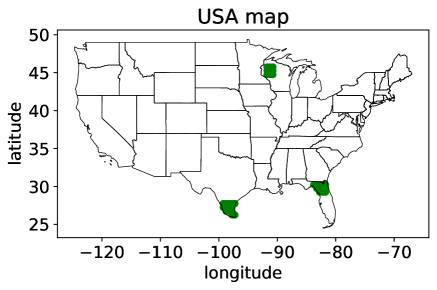
Figure 10: Regions where the temperature forecast is analyzed. See Section 8.4 for details. In Texas and Florida, the ensemble average performance drastically underperforms in the test set compared to both the training and validation sets. In Wisconsin, all methods show good performance. See Table 11.

Table 11: Train, validation, and test performance of different methods in Texas, Florida, and Wisconsin regions. The task is temperature regression; NCEP-CFSv2 dataset is used. The performance of the ensemble average and linear regression in the test period significantly decreases in Texas and Florida while the random forest is able to demonstrate reasonable results. All methods perform well in Wisconsin.

Region location	Model	Train mean $R^{2}$ ($\uparrow$)	Validation mean $R^{2}$ ($\uparrow$)	Test mean $R^{2}$ ($\uparrow$)
	Ens avg	0.19	0.36	-1.55
Texas	LR	0.53	0.49	-1.29
	RF	0.97	0.32	-0.33
	Ens avg	0.11	0.34	-0.87
Florida	LR	0.47	0.58	-0.56
	RF	0.97	0.36	0.11
	Ens avg	0.30	0.36	0.39
Wisconsin	LR	0.53	0.57	0.51
	RF	1.00	0.47	0.47

Why does RF perform so much better than simpler methods in some regions? One possibility is that the RF is a nonlinear model capable of more complex predictions. However, if that were the only cause of the discrepancy in performance, then we would expect that the RF would be better not only on the test period, but on the validation period as well. Table 11 does not support this argument; it shows that the ensemble average and linear regression have comparable if not superior performance to the random forest during the validation period. A second hypothesis is that the distribution of temperature is different during the test period than during the training and validation periods. This hypothesis is plausible for two reasons: (1) climate change, and (2) the training and validation data use hindcast ensembles while the test data uses forecast ensembles. To investigate this hypothesis, in Figure 11 we plot the true temperature and ensemble average in the training, validation, and test periods for the three geographic regions. The discrepancy between the true temperatures and ensemble averages in the test period is generally greater than during the training and validation periods in Texas and Florida (though not in Wisconsin, a region in which validation and test performance are comparable for all methods). This lends support to the hypothesis that hindcast and forecast ensembles exhibit distribution drift, and the superior performance of the RF during the test period may be due to a greater robustness to that distribution drift.

The hindcast and forecast ensembles may have different predictive accuracies because the hindcast ensembles have been debiased to fit past climate data – a procedure not possible for forecast data. To explore the potential impact of debiasing, Figure 11 shows the “oracle debiased ensemble average”, which is computed by using the test data to estimate the forecast ensemble bias and subtract it from the ensemble average. This procedure, which would not be possible in practice and is used only to probe distribution drift ensemble bias, yields smaller discrepancies between the true data and the (oracle debiased) ensemble average than the discrepancies between the true data and the original (biased) ensemble average. Specifically, the oracle ensemble member achieves -0.20 mean $R^{2}$ score (TX) and -0.28 mean $R^{2}$ score (FL) vs. -1.55 $R^{2}$ (TX) and -0.87 $R^{2}$ (FL) of the original forecast ensemble average. The errors during the test period are generally larger than during the train and validation period, even after debiasing the ensemble members using future data. This effect may be attributed both to (a) the nonstationarity of the climate (note that there are more extreme values during the test period than during the training and validation periods, particularly in Texas and Florida) and (b) the fact that in the train and validation periods, we use hindcast ensemble members, whereas in the test period, we use forecast ensemble members.

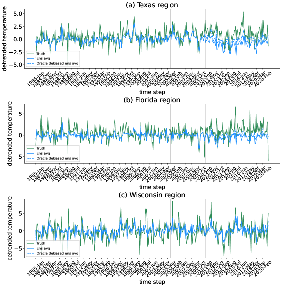
Figure 11: Temperature predictions in ${}^{\circ}C$ of different methods at Texas, Florida, and Wisconsin regions. Black lines correspond to train/val and val/test splits; train and validation correspond to the hindcast regime of the ensemble, while test corresponds to the forecast regime. See Section 8.4 for details.

9 Conclusions and future directions

This paper systematically explores the use of machine learning methods for subseasonal climate forecasting, highlighting several important factors: (1) the importance of using full ensembles of physics-based climate forecasts (as opposed to only using the mean, as in common practice); (2) the potential for forecasting extreme climate using quantile regression; (3) the efficacy of different mechanisms, such as positional encoding and convolutional neural networks, for modeling spatial dependencies; (4) the importance of various features, such as sea surface temperature and lagged temperature and precipitation values, for predictive accuracy. Together, these results provide new insights into using ML for subseasonal climate forecasting in terms of the selection of features, models, and methods.

Our results also suggest several important directions of future research. In terms of features, there are many climate forecasting ensembles computed by organizations such as NOAA and ECMWF. This paper focuses on ensembles in which ensemble members have a distinct ordering (in terms of lagged initial conditions used to generate them), but other ensembles correspond to initial conditions or parameters drawn independently from some distribution. Leveraging such ensemble forecasts, and potentially jointly leveraging ensemble members from multiple distinct ensembles, may further improve the predictive accuracy of our methods.

In terms of models, new neural architecture models such as transformers have shown remarkable performance on a number of image analysis tasks [54, 55, 56, 49] and have potential in the context of forecasting climate temperature and precipitation maps. Careful study is needed, as past image analysis work using transformers generally uses large quantities of training data, exceeding what is available in SSF contexts.

In terms of methods, two outstanding challenges are particularly salient to the SSF community. The first is uncertainty quantification; that is, we wish not only to forecast temperature or precipitation, but also to predict the likelihood of certain extreme events. Our work on quantile regression is an important step in this direction, and statistical methods like conformal quantile regression [57] may provide additional insights. Second, we see in Fig. 11 that, at least in some geographic regions, the distribution of ensemble hindcast and forecast data may be quite different. Employing methods that are more robust to distribution drift [58, 59, 60] is particularly important not only to handling forecast and hindcast data, but also for accurate SSF in a changing climate.

Appendix A Results for NASA-GMAO Dataset

A.1 Regression

Precipitation regression

Precipitation regression results on the test data from NASA-GMAO are presented in Table 12. On this dataset, no learned method or method leveraging ensemble model forecasts outperforms the historical average model significantly. Note that the best $R^{2}$ value, associated with the historical average, is still negative; the low values for all methods indicate the difficulty of the forecasting problem.

Table 12: Test results for precipitation regression using NASA-GMAO dataset. LR refers to linear regression on all features including ensemble members, lagged data, land variables, and SSTs. Model stacking is performed on models that are learned on all features. Bold values indicate the best performance for each statistic. MSE is reported in mm.

Model	Features	Mean $R^{2}$ ($\uparrow$)	Median $R^{2}$ ($\uparrow$)	Mean Sq Err ($\downarrow$)	Median MSE ($\downarrow$)	90th prctl MSE ($\downarrow$)
	Historical avg	-0.07	-0.02	2.14 $\pm$ 0.04	1.51	4.40
	Ens avg	-0.11	-0.06	2.13 $\pm$ 0.04	1.52	4.31
Baseline	Linear Regr	-0.18	-0.14	2.25 $\pm$ 0.04	1.62	4.68
LR	All features	-0.40	-0.29	2.62 $\pm$ 0.05	1.93	5.42
U-Net	All features	-0.19	-0.09	2.11 $\pm$ 0.03	1.56	4.25
RF	All features	-0.18	-0.11	2.17 $\pm$ 0.04	1.55	4.44
Stacked	LR, U-Net, RF, outputs	-0.08	-0.06	2.09 $\pm$ 0.04	1.52	4.27

Figure 12 illustrates test performance of key methods on NCEP-CFSv2 data with $R^{2}$ heatmaps over the U.S. Although the stacked model does not show the best performance in terms of mean $R^{2}$ score, it has more geographic regions with positive $R^{2}$ than any other method.

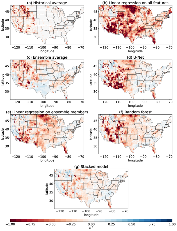
Figure 12: Test $R^{2}$ score heatmaps of baselines and learning-based methods for precipitation regression using the NASA-GMAO dataset. Positive values (blue) indicate better performance. See Section A.1 for details.

Regression of temperature

Temperature regression results using NASA-GMAO ensemble members are presented in Table 13. The random forest and linear regression outperform all baselines in terms of both $R^{2}$ score and MSE. However, the U-Net model’s performance is lower compared to other learned methods, which might be a sign of overfitting. Despite this performance drop of U-Net, the model stacking approach demonstrates the best predictive skill. Note that the model stacking approach is applied to the models that are trained on all available features except SSTs (similar to NCEP-CFSv2 data).

Table 13: Test results for temperature regression using NASA-GMAO dataset. LR refers to linear regression on all features including ensemble members, lagged data, and land variables. Model stacking is performed on models that are learned on all features except SSTs. Bold values indicate the best performance for each statistic. MSE is reported in ${}^{\circ}C$.

Model	Features	Mean $R^{2}$ ($\uparrow$)	Median $R^{2}$ ($\uparrow$)	Mean Sq Err ($\downarrow$)	Median MSE ($\downarrow$)	90th prctl MSE ($\downarrow$)
	Historical avg	-0.70	-0.20	6.49 $\pm$ 0.11	5.06	9.72
	Ens avg	-0.28	0.12	4.82 $\pm$ 0.10	3.43	7.82
Baseline	Linear Regr	0.12	0.14	3.32 $\pm$ 0.02	3.11	4.70
LR	All features wo SSTs	0.17	0.17	3.10$\pm$ 0.02	3.05	4.26
U-Net	All features wo SSTs	0.06	0.12	3.40 $\pm$ 0.02	3.27	4.52
RF	All features wo SSTs	0.20	0.22	3.03 $\pm$ 0.02	2.94	4.25
Stacked	LR, U-Net, RF, outputs	0.21	0.22	2.94 $\pm$ 0.02	2.89	3.97

Figure 13 illustrates the test performance of key methods on NASA-GMAO data with $R^{2}$ heatmaps over the U.S. The stacked model shows the best performance across spatial locations. Similar to the NCEP-CFSv2 dataset, we notice that there are still regions where all models tend to exhibit a negative $R^{2}$ score.

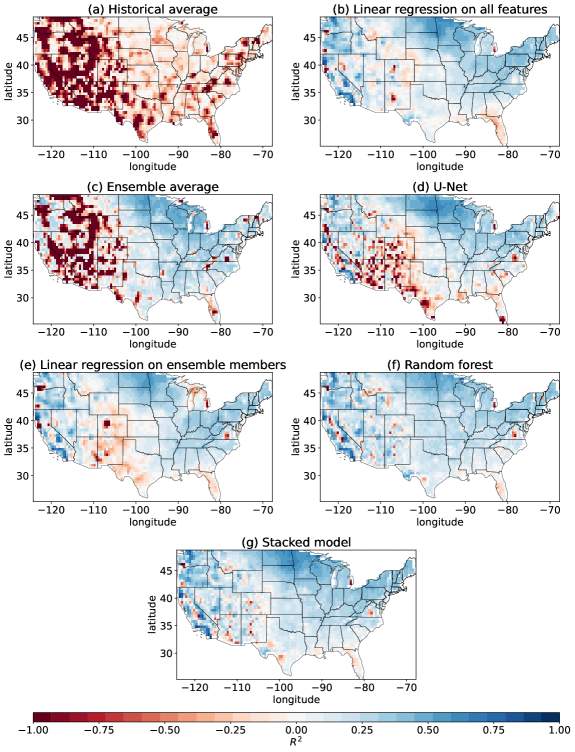
Figure 13: Test $R^{2}$ score heatmaps of baselines and learning-based methods for temperature regression using NASA-GMAO dataset. Positive values (blue) indicate better performance. See Section A.1 for details.

A.2 Quantile regression

Quantile regression of precipitation

Table 14 summarizes results for precipitation quantile regression using the NASA-GMAO ensemble. The models are the same as the models applied to the NCEP-CFSv2 ensemble. Our best model shows similar performance to that of the baselines. One possible reason is that the NASA-GMAO ensemble shows worse performance than the NCEP-CFSv2 ensemble empirically. Furthermore, according to the designs of ensemble members from both climate models, the NASA-GMAO ensemble has fewer ensemble members and therefore has less coverage on the distribution of precipitation than the NCEP-CFSv2 ensemble, so that our learned model has access to less information about the true distribution of precipitation.

Table 14: Test results for precipitation quantile regression using NASA-GMAO dataset, with target quantile = 0.9. Model stacking is performed on models that are learned on all features.

Model	Features	Mean Qtr Loss ($\downarrow$)	Median Qtr Loss ($\downarrow$)	90th prctl Qtr Loss ($\downarrow$)
	Historical 90-th percentile	0.295 $\pm$ 0.003	0.263	0.484
	Ens 90-th percentile	0.378$\pm$ 0.005	0.308	0.673
Baseline	Linear QR ens only	0.336 $\pm$ 0.004	0.286	0.531
Linear QR	All features	0.290 $\pm$ 0.003	0.253	0.456
U-Net	All features	0.310 $\pm$ 0.002	0.278	0.489
RFQR	All features	0.290 $\pm$ 0.002	0.265	0.471
Stacked	U-Net, RFQR, LQR outputs	0.296$\pm$ 0.002	0.268	0.467

Quantile regression of temperature

Table 15 summarizes results for temperature quantile regression using the NASA-GMAO ensemble. All of our learned models are able to outperform all baselines.

Table 15: Test results for temperature quantile regression using NASA-GMAO dataset, with target quantile = 0.9. Linear QR refers to a linear quantile regressor, i.e. linear regression fitting the quantile loss, using all features including ensemble members, positional encoding, lagged data, land variables. Model stacking is performed on models that are learned on all features except for SSTs .

Model	Features	Mean Qtr Loss ($\downarrow$)	Median Qtr Loss ($\downarrow$)	90th prctl Qtr Loss ($\downarrow$)
	Historical 90-th percentile	0.596 $\pm$ 0.010	0.438	0.988
	Ens 90-th percentile	0.812 $\pm$ 0.009	0.646	1.493
Baseline	Linear QR ens only	0.445 $\pm$ 0.003	0.411	0.618
Linear QR	All features wo SSTs	0.341 $\pm$ 0.001	0.333	0.419
U-Net	All features wo SSTs	0.375 $\pm$ 0.003	0.347	0.477
RFQR	All features wo SSTs	0.318 $\pm$ 0.002	0.316	0.376
Stacked	U-Net, RFQR, LQR outputs	0.315 $\pm$ 0.002	0.310	0.374

Figure 15: Test quantile loss heatmaps of baselines and learning-based methods for temperature quantile regression using NASA-GMAO dataset. Blue regions indicate smaller quantile loss. See Section A.2 for details.

Appendix B Tercile Classification

In this section, we present results for the tercile classification task for both climate variables and both datasets.

B.1 Tercile classification of precipitation

In this case, the proposed learning-based methods are trained on the classification task directly. Predictions of baselines, such as the ensemble average, are split into three classes according to the 33rd and 66th percentile values. Note that random forest and U-Net are trained for classification using all available features. We do not notice a significant difference in performance of logistic regression on the validation if the inputs are ensemble members only or ensemble members with side information. So, we use logistic regression on ensemble members only. The model stacking is applied to the logistic regression, U-Net and random forest outputs.

Table 16 summarizes results for NCEP-CFSv2 and NASA-GMAO datasets on the test data. For this task, the learning-based methods achieve the best performance in terms of accuracy for both datasets. In the case of NCEP-CFSv2 data, U-Net achieves the highest accuracy score, and the performance of the stacked model is comparable with it. For NASA-GMAO data, the stacked model shows the best performance.

Table 16: Test results for tercile classification of precipitation on different datasets. Accuracy in % is reported. Note that for this task, our models are trained for classification directly while baselines perform regression and threshold for predicted values is applied. For stacking, logistic regression, U-Net and RF outputs are used.

Data	Model	Mean accuracy ($\uparrow$)	Median accuracy ($\uparrow$)
	Ens avg	38.00 $\pm$0.16	37.61
	Logistic Regr	41.22 $\pm$0.14	40.17
NCEP-CFSv2	U-Net	43.88 $\pm$0.12	42.74
	RF	42.38 $\pm$0.13	41.88
	Stacked	43.81 $\pm$0.13	42.74
	Ens avg	38.64 $\pm$0.14	37.65
	Logistic regr	41.51 $\pm$0.16	40.00
NASA-GMAO	U-Net	40.53 $\pm$0.11	40.00
	RF	40.79 $\pm$0.14	40.00
	Stacked	42.08 $\pm$0.14	41.18

The accuracy heatmaps over U. S. land are presented in the Figure 16 for NCEP-CFSv2 dataset. The plots corresponding to the learning-based methods show the best results, especially at the West Coast, Colorado and North America.

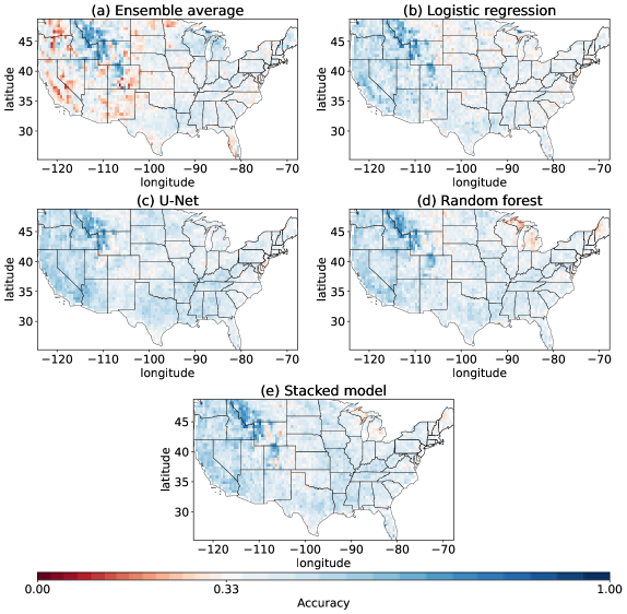
Figure 16: Test accuracy heatmaps of baselines and learning-based methods for tercile classification of precipitation using NCEP-CFSv2 dataset. The accuracy colorbar is recentered to be white at $\frac{1}{3}$, what corresponds to a random guess score. Blue pixels indicate better performance, while red pixels correspond to performance that is worse than a random guess. See Section B.1 for details.

The accuracy heatmaps over U. S. land are presented in the Figure 17 for NASA-GMAO dataset. The plots corresponding to the learning-based methods show the best results, the ensemble average’s figure has the most red regions.

Figure 17: Test accuracy heatmaps of baselines and learning-based methods for tercile classification of precipitation using NASA-GMAO dataset. The accuracy colorbar is recentered to be white at $\frac{1}{3}$, what corresponds to a random guess score. Blue pixels indicate better performance, while red pixels correspond to performance that is worse than a random guess. See Section B.1 for details.

B.2 Tercile classification of temperature

The next task is tercile classification of 2-meter temperature. In this case, the threshold is applied to the regression predictions of all methods, meaning there is no direct training for a classification. Table 17 summarizes results for NCEP-CFSv2 and NASA-GMAO datasets on the test data. For this task, the learning-based methods achieve the best performance in terms of accuracy, stacked model using NCEP-CFSv2 data and linear regression using NASA-GMAO data and all additional features (except SSTs). In general, all learning-based models significantly outperform the ensemble average.

Table 17: Test results for tercile classification of temperature on different datasets. Accuracy in % is reported. Note that for this task, our models are trained for regression and the threshold for predicted values is applied.

Data	Model	Mean accuracy ($\uparrow$)	Median accuracy ($\uparrow$)
	Ens avg	44.84 $\pm$0.36	42.74
	Linear Regr	57.10 $\pm$0.25	54.69
NCEP-CFSv2	LR	57.34 $\pm$0.25	54.71
	U-Net	53.80 $\pm$0.28	50.43
	RF	58.07 $\pm$0.27	54.70
	Stacked	58.12 $\pm$0.20	54.71
	Ens avg	52.23 $\pm$0.25	49.41
	Linear Regr	57.75 $\pm$0.25	54.11
NASA-GMAO	LR	58.97 $\pm$0.25	55.29
	U-Net	55.64 $\pm$0.27	51.76
	RF	58.78 $\pm$0.26	55.29
	Stacked	58.72 $\pm$0.25	54.12

Figure 18 shows accuracy heatmaps over the U.S. for different methods using NCEP-CFSv2 data. The stacked model shows the best performance across spatial locations. For example, the ensemble average does not show great performance in the South East and Middle Atlantic regions, while learning based methods demonstrate much stronger predictive skill in these areas. However, there are still some areas, such as Texas or South West region, with red pixels for all methods.

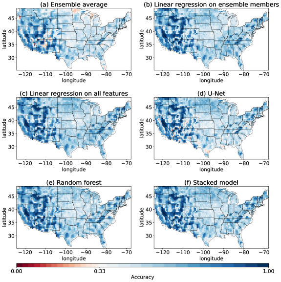
Figure 18: Test accuracy heatmaps of baselines and learning-based methods for tercile classification of temperature using NCEP-CFSv2 dataset. The accuracy colorbar is recentered to be white at $\frac{1}{3}$, what corresponds to a random guess score. Blue pixels indicate better performance, while red pixels correspond to performance that is worse than a random guess. See Section B.2 for details.

Figure 19 shows accuracy heatmaps over the U.S. for different methods using NASA-GMAO data. In this case, linear regression on all features achieves the best scores. Other learning-based methods outperform the ensemble average too, especially in the West and in Minnesota.

Figure 19: Test accuracy heatmaps of baselines and learning-based methods for tercile classification of temperature using NASA-GMAO dataset. The accuracy colorbar is recentered to be white at $\frac{1}{3}$, what corresponds to a random guess score. Blue pixels indicate better performance, while red pixels correspond to performance that is worse than a random guess. See Section B.2 for details.

Appendix C Extended Discussions

In this section, we present more detailed results for Section 8.

C.1 Full ensemble v.s. ensemble average and sorted ensemble

In Section 8.1, we show a set of experiments with different usage of the ensemble. In particular, we compare our model performance when for using only the ensemble average, using the sorted ensemble or using the full ensemble, along with all other features. In Table 18 we further show the results for all our machine learning models, i.e., LR, RF, U-Net and stacked model under these three settings. For linear regression, using the ensemble average with all other features produces the best test performance, compared to using the sorted ensemble or the full ensemble. This is not surprising for the LR, since the full ensemble incorporates large variance across ensemble members, which may result in a worse linear fit. For the U-Net, RF and stacked model, we observe significant performance improvement, in terms of having at least one standard error smaller MSE, when using the full ensemble instead of using the ensemble average or the sorted ensemble. This shows evidence that the non-linear machine learning models we show here, including U-Net, RF and stacked model, are able to leverage the extra information in these ensemble members and produce better predictions than only using the ensemble average. We also present the $R^{2}$ heatmaps for all our machine learning models under these three settings with the ensemble in Figure 20. We can see clear improvement for the U-Net, RF and stacked model from using ensemble average to using the full ensemble. This also shows that our stacked model is able to gain from better model outputs of RF and U-Net.

Table 18: Precipitation regression test performance comparison of LR, U-Net, RF and stacked model trained using ensemble average only, using sorted ensemble or using the full ensemble. The best results are in bold.

Model	Features	Mean $R^{2}$ ($\uparrow$)	Mean Sq Err ($\downarrow$)
	Ensemble avg + all features	-0.28	2.59$\pm$0.04
LR	Sorted ensemble + all features	-0.43	2.87$\pm$0.05
	Full ensemble + all features	-0.33	2.71$\pm$0.05
	Ensemble avg + all features	-0.45	2.76$\pm$0.04
U-Net	Sorted ensemble + all features	-0.45	2.78$\pm$0.04
	Full ensemble + all features	-0.1	2.18$\pm$0.03
	Ensemble avg + all features	-0.16	2.36$\pm$0.04
RF	Sorted ensemble + all features	-0.18	2.30$\pm$0.04
	Full ensemble + all features	-0.11	2.17$\pm$0.05
	Ensemble avg + all features	-0.08	2.28$\pm$0.04
Stacked	Sorted ensemble + all features	-0.11	2.24$\pm$0.04
	Full ensemble + all features	0.02	2.07$\pm$0.03

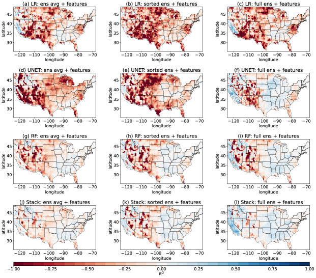
Figure 20: Precipitation regression test $R^{2}$ heatmaps of LR, U-Net, RF and stacked model trained using ensemble average only, using sorted ensemble or using the full ensemble. The NCEP-CFSv2 ensemble is used.

The experiment results for temperature regression on the same settings are shown in Table 19. Similar to the precipitation regression results, having the full ensemble does not show noticeable improvement for the LR, but it significantly improves model performance for the U-Net, RF and stacked model. Specifically for the U-Net, using the sorted ensemble drastically degrades its performance, which is essentially because we sort the ensemble members for each location individually, as we describe in Section 8.1, and sorting the ensemble members individually for each location may break the spatial correlations that the U-Net is learning.

Again, we visually show the $R^{2}$ heatmaps for this experiment in Figure 21. It’s clear to see that the U-Net’s performance degrades when using the sorted ensemble. Other than that, the results are consistent with what we observe in the precipitation regression results, which is the U-Net, RF and stacked model’s performances improve when using the full ensemble compared to using the ensemble average or the sorted ensemble, and the stacked model is able to capture those improvements from the U-Net and RF.

Table 19: Temperature regression test performance comparison of LR, U-Net, RF and stacked model trained using ensemble average only, using sorted ensemble or using the full ensemble. The best results are in bold.

Model	Features	Mean $R^{2}$ ($\uparrow$)	Mean Sq Err ($\downarrow$)
	Ensemble avg + all features	0.06	3.55$\pm$0.03
LR	Sorted ensemble + all features	-0.02	3.87$\pm$0.03
	Full ensemble + all features	0.05	3.57$\pm$0.02
	Ensemble avg + all features	0.00	3.77$\pm$0.03
U-Net	Sorted ensemble + all features	-0.94	6.51$\pm$0.05
	Full ensemble + all features	0.01	3.65$\pm$0.02
	Ensemble avg + all features	0.10	3.57$\pm$0.02
RF	Sorted ensemble + all features	0.10	3.44$\pm$0.02
	Full ensemble + all features	0.16	3.17$\pm$0.02
	Ensemble avg + all features	0.11	3.35$\pm$0.02
Stacked	Sorted ensemble + all features	0.03	3.70$\pm$0.02
	Full ensemble + all features	0.18	3.11$\pm$0.02

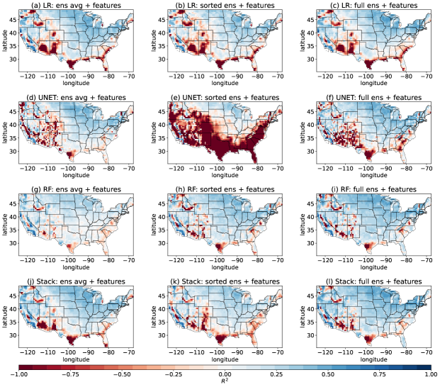
Figure 21: Temperature regression test $R^{2}$ heatmaps of LR, U-Net, RF and stacked model trained using ensemble average only, using sorted ensemble or using the full ensemble. The NCEP-CFSv2 ensemble is used.

C.2 PE v.s. latitude/longitude values or no location information

In this section, we elaborate on our experiment with different usage of location information. Similar to Section 8.2, we train and test our models with three different settings: using no location information, using latitude/longitude values or using positional encodings. For the stacked model, we first train the LR, RF and U-Net using these different settings, before training the stacked model using the corresponding LR, RF and U-Net outputs. Table 20 summarizes test performance for precipitation regression with these three settings of using location information. For Linear regression, we observe that having latitude/longitude values or adding PE features does not improve its performance. One interesting result is that adding PE for the LR degraded its performance, which may due to that the PE features are non-linear transformations of latitude and longitude values, which is hard to fit with a linear model.

For the RF, U-Net and the stacked model, we observe that adding PE improves their performance with significance, i.e. having at least one standard error smaller MSE. For the U-Net, using latitude/longitude values yields worse overall performance compared to using no location information, potentially due to that the latitude/longitude values are discrete values, whereas the PE values are smooth across space. Figure 22 shows the test $R^{2}$ heatmaps for LR, U-Net, RF and stacked model under these three settings for precipitation regression. We observe that adding PE features not only improves performance for the U-Net and RF, the stacked model’s performance also improves from having better predictions from the U-Net and RF.

Table 20: Precipitation regression test performance comparison of LR, U-Net, RF and stacked model trained using no spatial features, using latitude and longitude values or using PE. The best results are in bold.

Model	Features	Mean $R^{2}$ ($\uparrow$)	Mean Sq Err ($\downarrow$)
	All + no location info	-0.11	2.29$\pm$0.04
LR	All + lat/lon values	-0.11	2.29$\pm$0.04
	All + PE	-0.33	2.71$\pm$0.05
	All + no location info	-0.16	2.31$\pm$0.04
U-Net	All + lat/lon values	-0.28	2.53$\pm$0.05
	All + PE	-0.10	2.18$\pm$ 0.03
	All + no location info	-0.18	2.23$\pm$0.04
RF	All + lat/lon values	-0.16	2.21$\pm$0.04
	All + PE	-0.11	2.17$\pm$ 0.05
	All + no location info	-0.05	2.13$\pm$0.03
Stacked	All + lat/lon values	-0.01	2.21$\pm$0.04
	All + PE	0.02	2.07$\pm$ 0.03

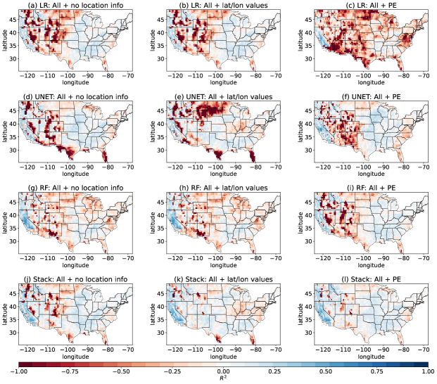
Figure 22: Precipitation regression test $R^{2}$ heatmaps of LR, U-Net, RF and stacked model trained using no spatial features, using latitude and longitude values or using PE. The NCEP-CFSv2 ensemble is used.

Table 21 shows the test performances of LR, U-Net, RF and stacked model on temperature regression. Similar to precipitation regression, adding latitude/longitude values or adding PE does not help the LR, but we observe significant performance improvement when adding positional encodings features for the U-Net, RF and the stacked model. Figure 23 then shows the test $R^{2}$ heatmaps for temperature regression. We can see that adding PE to the U-Net, RF and stacked model improves forecast performance, especially in regions like Arizona, New Mexico and Texas.

Table 21: Temperature regression test performance comparison of LR, U-Net, RF and stacked model trained using no spatial features, using latitude and longitude values or using PE. The best results are in bold.

Model	Features	Mean $R^{2}$ ($\uparrow$)	Mean Sq Err ($\downarrow$)
	All + no location info	0.05	3.57$\pm$0.03
LR	All + lat/lon values	0.05	3.57$\pm$0.03
	All + PE	0.05	3.57$\pm$0.03
	All + no location info	-0.35	4.81$\pm$0.04
U-Net	All + lat/lon values	-0.21	4.47$\pm$0.03
	All + PE	0.01	3.65$\pm$ 0.02
	All + no location info	0.11	3.37$\pm$0.02
RF	All + lat/lon values	0.14	3.28$\pm$0.02
	All + PE	0.16	3.17$\pm$ 0.02
	All + no location info	0.12	3.35$\pm$0.02
Stacked	All + lat/lon values	0.12	3.33$\pm$0.02
	All + PE	0.18	3.11$\pm$ 0.02

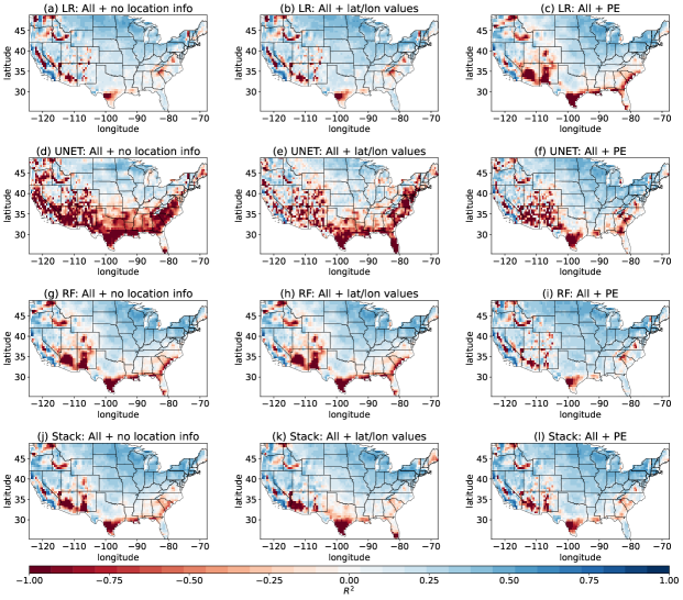
Figure 23: Temperature regression test $R^{2}$ heatmaps of LR, U-Net, RF and stacked model trained using no spatial features, using latitude and longitude values or using PE. The NCEP-CFSv2 ensemble is used.

C.3 Bootstrap experiments

To evaluate the stability of our machine learning models with small sample sizes, we perform the following bootstrap experiments: We take bootstrap samples of size 200 from our training set and retrain our U-Net, RF and LR. Then we evaluate these models on the test set. We repeat this process for 50 times and show the results in Figure 24. We observe from the plots that the U-Net performs consistently better than the LR in precipitation regression, but not for temperature regression. This result is consistent with what we showed in Table 3 and Table 4.

We also observe that the U-Net is more sensitive to different bootstrap samples than the RF and LR, which is not surprising since for the U-Net, the bootstrap samples correspond to 200 different spatial maps for training. In contrast, for the RF and LR, the bootstrap samples correspond to $200\cdot 3274$ training samples.

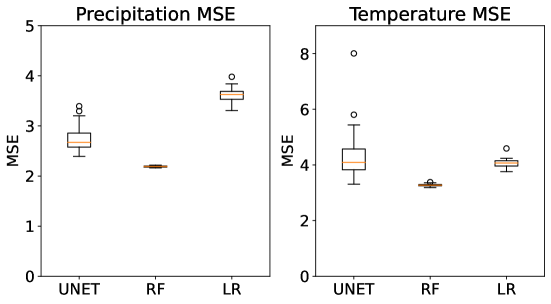
Figure 24: Box plots of MSEs for the U-Net, LR and RF trained on 50 set of different bootstrap samples, each with size 200. The NCEP-CFSv2 ensemble is used.

Appendix D Architecture Details

U-Net details

The U-Net has residual connections from layers in the encoder part to the decoder part in a paired way so that it forms a U-shape. Figure 25 shows the architecture of the U-Net. The U-Net is a powerful deep convolutional network that is widely used in image processing tasks such as image segmentation and image classification.

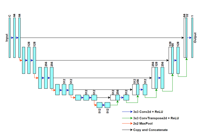
Figure 25: U-Net architecture with input channels = $C$. $C$ is the number of input channels, which in our case equals the number of ensemble members plus all climate data.

Our U-Net differs from the original U-Net by modifying the first 2D convolutional layer after input. Since our input channels can be different when we choose a different subset of features or different ensemble (NCEP-CFSv2 or NASA-GMAO), this 2D convolutional layer is used to transform our input with $C$ channels into a latent representation with 64 channels. The number of channels $C$ depends on which ensemble we are using, and what task we are performing. For example, for precipitation tasks using the NCEP-CFSv2 ensemble, the input channels include $24$ ensemble members, $5$ lagged observations, $4$ other observational variables, $8$ principal components of SSTs, and 24 positional encoding, resulting in $65$ channels in total. For temperature tasks using the NASA-GMAO ensemble, there are only $11$ ensemble members, and we don’t include SSTs information, hence there are only $44$ channels in total. The other following layers use the same configurations with the standard U-Net [39].

We also perform careful hyperparameter tuning for the U-NET. In particular, we run 10-fold cross validation on our training set, and use grid search for tuning learning rate, batch size, number of epochs, and weight decay. Since we use different loss functions for different forecast tasks and different number of input channels for NCEP-CFSv2 and GMAO-GMAO ensemble, we run hyperparameter tuning with the same cross validation scheme separately for these tasks. For instance, for precipitation regression, we choose from 100, 120, 150, 170, 200, 250 epochs; batch size may be equal to 8, 16, 32; learning rate values are chosen from 0.0001, 0.001, 0.01; weight decay can be 0, 1e-3, 1e-4. In case of NCEP-CFSv2 precipitation regression, the optimal parameters are 170 epochs, batch size 16, learning rate 0.0001, and weight decay 1e-4. For temperature regression using the same data, the best parameters are: 100 epochs, batch size 16, learning rate 0.001, and weight decay 1e-3. For tercile classification of precipitation, the best parameters are 80 epochs (we chose from 60, 70, 80, 90, 100 epochs during classification), batch size 8, learning rate 0.001, and weight decay 1e-4.

Random Forest Quantile Regressor details

We show a figure representation of the RFQR in Figure 26. The RFQR is essentially trained as a regular random forest, but it makes a quantile estimate by taking the sample quantile of the responses in all leaves associated with a new input.

Figure 26: Illustration of a Random Forest, which serves as a visual aid for the ensuing discussion on existing and proposed methods. Quantile Regression Forests outputs the empirical $\alpha$ quantiles of the collection of all responses in all the leaves associated with $\mathbf{x}_{t,l}$ (marked with a star for each tree).

Stacking model details

The stacking model is a simple one layer neural network with 100 hidden neurons and sigmoid activation function for regression and softmax for classification. We use an implementation from Scikit-learn library [38]. We choose 100 neurons based on the stacking model performance on the validation data (we also try 50, 75, 100 and 120 neurons). The stacking model demonstrates stable performance in general, but with 100 neurons it usually achieves the best results. We use ”lbfgs” optimizer from quasi-Newton methods for the regression tasks, and SGD optimizer for classification tasks.

Appendix E Additional Preprocessing Details

Random forest and U-Net require different input formats. For U-Net, all input variables have natural image representation except SSTs and information about location. For example, ensemble predictions can be represented as a tensor of shape $(K,W,H)$, where $K$ corresponds to the number of ensemble members (or number of channels of an image), and $W$ and $H$ are width and height of the corresponding image. In our case, $W=64$ and $H=128$. For the U-Net model, we handle the missing land variables over the sea regions by the nearest neighbor interpolation of available values.

Sea surface temperatures

There are more than 100,000 SSTs locations available. We extract the top eight principal components. Principal component analysis fits on train part and then is applied for the rest of the data. In the case of U-Net, we deal with PCs of SSTs by adding additional input channels that are constant across space with each channel corresponding to one of PCs. Random forest can use PCs from SSTs directly with no special preprocessing.

Normalization

We apply channel-wise min-max normalization to the input features at each location based on training part of the dataset in the case of U-Net. As for normalization of the true values, min-max normalization is applied for precipitation and standardization is applied for temperature. This choice affects the final layer of U-Net model too: for the precipitation regression task, the sigmoid activation is used, and no activation function is applied for temperature regression. For the staking model, we apply min-max normalization to both input and target values.

References

- Ban et al. [2016] R. J Ban, C. M. Bitz, A. Brown, E. Chassignet, J. A. Dutton, R. Hallberg, A. Kamrath, D. Kleist, P. F. J. Lermusiaux, H. Lin, L. Myers, J. Pullen, S. Sandgathe, M. Shafer, D. Waliser, and C. Zhang. Next Generation Earth System Prediction: Strategies for Subseasonal to Seasonal Forecasts. The National Academies Press, 2016.
- Lorenc [1986] Andrew C Lorenc. Analysis methods for numerical weather prediction. Quarterly Journal of the Royal Meteorological Society, 112(474):1177–1194, 1986.
- National Academies of Sciences [2016] National Academies of Sciences. Next generation earth system prediction: strategies for subseasonal to seasonal forecasts. National Academies Press, 2016.
- National Research Council [2010] National Research Council. Assessment of intraseasonal to interannual climate prediction and predictability. National Academies Press, 2010.
- Simmons and Hollingsworth [2002] A. J. Simmons and A. Hollingsworth. Some aspects of the improvement in skill of numerical weather prediction. Quarterly Journal of the Royal Meteorological Society, 128(580):647–677, 2002.
- Barnston et al. [2012a] Anthony G. Barnston, Michael K. Tippett, Michelle L. L’Heureux, Shuhua Li, and David G. DeWitt. Skill of Real-time Seasonal ENSO Model Predictions during 2002–2011. Is Our Capability Increasing? Bull. Amer. Meteor. Soc., 93:631–651, 2012a.
- Council [2010] National Research Council. Assessment of intraseasonal to interannual climate prediction and predictability. National Academies Press, 2010.
- Hwang et al. [2018] Jessica Hwang, Paulo Orenstein, Karl Pfeiffer, Judah Cohen, and Lester Mackey. Improving subseasonal forecasting in the western us with machine learning. arXiv preprint arXiv:1809.07394, 2018.
- Hwang et al. [2019] Jessica Hwang, Paulo Orenstein, Judah Cohen, Karl Pfeiffer, and Lester Mackey. Improving subseasonal forecasting in the western us with machine learning. In Proceedings of the 25th ACM SIGKDD International Conference on Knowledge Discovery & Data Mining, pages 2325–2335, 2019.
- Kirtman et al. [2014] Ben P Kirtman, Dughong Min, Johnna M Infanti, James L Kinter, Daniel A Paolino, Qin Zhang, Huug Van Den Dool, Suranjana Saha, Malaquias Pena Mendez, Emily Becker, et al. The north american multimodel ensemble: phase-1 seasonal-to-interannual prediction; phase-2 toward developing intraseasonal prediction. Bulletin of the American Meteorological Society, 95(4):585–601, 2014.
- Saha et al. [2014] Suranjana Saha, Shrinivas Moorthi, Xingren Wu, Jiande Wang, Sudhir Nadiga, Patrick Tripp, David Behringer, Yu-Tai Hou, Hui-ya Chuang, Mark Iredell, et al. The ncep climate forecast system version 2. Journal of climate, 27(6):2185–2208, 2014.
- Nakada et al. [2018] Kazumi Nakada, Robin M Kovach, Jelena Marshak, and Andrea Molod. Global modeling and assimilation office - nasa, Apr 2018. URL https://gmao.gsfc.nasa.gov/pubs/docs/Nakada1033.pdf.
- Nebeker [1995] Frederik Nebeker. Calculating the weather: Meteorology in the 20th century. Elsevier, 1995.
- Barnston et al. [2012b] Anthony G Barnston, Michael K Tippett, Michelle L L’Heureux, Shuhua Li, and David G DeWitt. Skill of real-time seasonal enso model predictions during 2002–11: Is our capability increasing? Bulletin of the American Meteorological Society, 93(5):631–651, 2012b.
- Cofıno et al. [2002] Antonio S Cofıno, Rafael Cano, Carmen Sordo, and Jose M Gutierrez. Bayesian networks for probabilistic weather prediction. In 15th Eureopean Conference on Artificial Intelligence (ECAI). Citeseer, 2002.
- Ghaderi et al. [2017] Amir Ghaderi, Borhan M Sanandaji, and Faezeh Ghaderi. Deep forecast: Deep learning-based spatio-temporal forecasting. arXiv preprint arXiv:1707.08110, 2017.
- Grover et al. [2015] Aditya Grover, Ashish Kapoor, and Eric Horvitz. A deep hybrid model for weather forecasting. In Proceedings of the 21th ACM SIGKDD international conference on knowledge discovery and data mining, pages 379–386, 2015.
- Herman and Schumacher [2018] Gregory R Herman and Russ S Schumacher. “dendrology” in numerical weather prediction: What random forests and logistic regression tell us about forecasting extreme precipitation. Monthly Weather Review, 146(6):1785–1812, 2018.
- Radhika and Shashi [2009] Y Radhika and M Shashi. Atmospheric temperature prediction using support vector machines. International journal of computer theory and engineering, 1(1):55, 2009.
- Badr et al. [2014] Hamada S Badr, Benjamin F Zaitchik, and Seth D Guikema. Application of statistical models to the prediction of seasonal rainfall anomalies over the sahel. Journal of Applied meteorology and climatology, 53(3):614–636, 2014.
- Iglesias et al. [2015] Gilberto Iglesias, David C Kale, and Yan Liu. An examination of deep learning for extreme climate pattern analysis. In The 5th International Workshop on Climate Informatics, 2015.
- Cohen et al. [2019] Judah Cohen, Dim Coumou, Jessica Hwang, Lester Mackey, Paulo Orenstein, Sonja Totz, and Eli Tziperman. S2s reboot: An argument for greater inclusion of machine learning in subseasonal to seasonal forecasts. Wiley Interdisciplinary Reviews: Climate Change, 10(2):e00567, 2019.
- Totz et al. [2017] Sonja Totz, Eli Tziperman, Dim Coumou, Karl Pfeiffer, and Judah Cohen. Winter precipitation forecast in the european and mediterranean regions using cluster analysis. Geophysical Research Letters, 44(24):12–418, 2017.
- Vitart et al. [2012] Frédéric Vitart, Andrew W Robertson, and David LT Anderson. Subseasonal to seasonal prediction project: Bridging the gap between weather and climate. Bulletin of the World Meteorological Organization, 61(2):23, 2012.
- He et al. [2020] Sijie He, Xinyan Li, Timothy DelSole, Pradeep Ravikumar, and Arindam Banerjee. Sub-seasonal climate forecasting via machine learning: Challenges, analysis, and advances. arXiv preprint arXiv:2006.07972, 2020.
- Srinivasan et al. [2021] Vishwak Srinivasan, Justin Khim, Arindam Banerjee, and Pradeep Ravikumar. Subseasonal climate prediction in the western us using bayesian spatial models. In Uncertainty in artificial intelligence, pages 961–970. PMLR, 2021.
- He et al. [2021] Sijie He, Xinyan Li, Laurie Trenary, Benjamin A Cash, Timothy DelSole, and Arindam Banerjee. Learning and dynamical models for sub-seasonal climate forecasting: Comparison and collaboration. arXiv preprint arXiv:2110.05196, 2021.
- Grönquist et al. [2020] Peter Grönquist, Chengyuan Yao, Tal Ben-Nun, Nikoli Dryden, Peter Dueben, Shigang Li, and Torsten Hoefler. Deep learning for post-processing ensemble weather forecasts. CoRR, abs/2005.08748, 2020. URL https://arxiv.org/abs/2005.08748.
- Loken et al. [2022] Eric D. Loken, Adam J. Clark, and Amy McGovern. Comparing and interpreting differently designed random forests for next-day severe weather hazard prediction. Weather and Forecasting, 37(6):871 – 899, 2022. doi: https://doi.org/10.1175/WAF-D-21-0138.1. URL https://journals.ametsoc.org/view/journals/wefo/37/6/WAF-D-21-0138.1.xml.
- NOAA [2022] NOAA. Noaa national centers for environmental information, climate at a glance: National time series. https://www.ncdc.noaa.gov/cag/, 2022.
- Fan and Van den Dool [2008] Yun Fan and Huug Van den Dool. A global monthly land surface air temperature analysis for 1948–present. Journal of Geophysical Research: Atmospheres, 113(D1), 2008.
- Xie et al. [2010] P Xie, M Chen, and W Shi. Cpc global unified gauge-based analysis of daily precipitation. In Preprints, 24th Conf. on Hydrology, Atlanta, GA, Amer. Metero. Soc, volume 2, 2010.
- Reynolds et al. [2007] Richard W Reynolds, Thomas M Smith, Chunying Liu, Dudley B Chelton, Kenneth S Casey, and Michael G Schlax. Daily high-resolution-blended analyses for sea surface temperature. Journal of climate, 20(22):5473–5496, 2007.
- Kalnay et al. [1996] Eugenia Kalnay, Masao Kanamitsu, Robert Kistler, William Collins, Dennis Deaven, Lev Gandin, Mark Iredell, Suranjana Saha, Glenn White, John Woollen, et al. The ncep/ncar 40-year reanalysis project. Bulletin of the American meteorological Society, 77(3):437–472, 1996.
- Meinshausen [2006] Nicolai Meinshausen. Quantile regression forests. Journal of Machine Learning Research, 7(35):983–999, 2006. URL http://jmlr.org/papers/v7/meinshausen06a.html.
- Hastie et al. [2009] Trevor Hastie, Robert Tibshirani, Jerome H Friedman, and Jerome H Friedman. The elements of statistical learning: data mining, inference, and prediction, volume 2. Springer, 2009.
- Biau and Scornet [2016] Gérard Biau and Erwan Scornet. A random forest guided tour. Test, 25:197–227, 2016.
- Pedregosa et al. [2011] F. Pedregosa, G. Varoquaux, A. Gramfort, V. Michel, B. Thirion, O. Grisel, M. Blondel, P. Prettenhofer, R. Weiss, V. Dubourg, J. Vanderplas, A. Passos, D. Cournapeau, M. Brucher, M. Perrot, and E. Duchesnay. Scikit-learn: Machine learning in Python. Journal of Machine Learning Research, 12:2825–2830, 2011.
- Ronneberger et al. [2015] Olaf Ronneberger, Philipp Fischer, and Thomas Brox. U-net: Convolutional networks for biomedical image segmentation. In MICCAI, 2015.
- Yakubovskiy [2020] Pavel Yakubovskiy. Segmentation models pytorch. https://github.com/qubvel/segmentation_models.pytorch, 2020.
- Kingma and Ba [2014] Diederik P Kingma and Jimmy Ba. Adam: A method for stochastic optimization. arXiv preprint arXiv:1412.6980, 2014.
- Pavlyshenko [2018] Bohdan Pavlyshenko. Using stacking approaches for machine learning models. In 2018 IEEE Second International Conference on Data Stream Mining & Processing (DSMP), pages 255–258. IEEE, 2018.
- Vaswani et al. [2017] Ashish Vaswani, Noam Shazeer, Niki Parmar, Jakob Uszkoreit, Llion Jones, Aidan N Gomez, Łukasz Kaiser, and Illia Polosukhin. Attention is all you need. Advances in neural information processing systems, 30, 2017.
- Devlin et al. [2018] Jacob Devlin, Ming-Wei Chang, Kenton Lee, and Kristina Toutanova. Bert: Pre-training of deep bidirectional transformers for language understanding. arXiv preprint arXiv:1810.04805, 2018.
- Petroni et al. [2019] Fabio Petroni, Tim Rocktäschel, Patrick Lewis, Anton Bakhtin, Yuxiang Wu, Alexander H Miller, and Sebastian Riedel. Language models as knowledge bases? arXiv preprint arXiv:1909.01066, 2019.
- Narayanan et al. [2016] Annamalai Narayanan, Mahinthan Chandramohan, Lihui Chen, Yang Liu, and Santhoshkumar Saminathan. subgraph2vec: Learning distributed representations of rooted sub-graphs from large graphs. arXiv preprint arXiv:1606.08928, 2016.
- Gamboa [2017] John Cristian Borges Gamboa. Deep learning for time-series analysis. arXiv preprint arXiv:1701.01887, 2017.
- Gehring et al. [2017] Jonas Gehring, Michael Auli, David Grangier, Denis Yarats, and Yann N Dauphin. Convolutional sequence to sequence learning. In International conference on machine learning, pages 1243–1252. PMLR, 2017.
- Khan et al. [2022] Salman Khan, Muzammal Naseer, Munawar Hayat, Syed Waqas Zamir, Fahad Shahbaz Khan, and Mubarak Shah. Transformers in vision: A survey. ACM computing surveys (CSUR), 54(10s):1–41, 2022.
- Knapp et al. [2011] Kenneth R Knapp, Steve Ansari, Caroline L Bain, Mark A Bourassa, Michael J Dickinson, Chris Funk, Chip N Helms, Christopher C Hennon, Christopher D Holmes, George J Huffman, et al. Globally gridded satellite observations for climate studies. Bulletin of the American Meteorological Society, 92(7):893–907, 2011.
- Cash et al. [2019] Benjamin A Cash, Julia V Manganello, and James L Kinter. Evaluation of nmme temperature and precipitation bias and forecast skill for south asia. Climate dynamics, 53:7363–7380, 2019.
- Mamalakis et al. [2018] Antonios Mamalakis, Jin-Yi Yu, James T Randerson, Amir AghaKouchak, and Efi Foufoula-Georgiou. A new interhemispheric teleconnection increases predictability of winter precipitation in southwestern us. Nature communications, 9(1):2332, 2018.
- Seager et al. [2007] Richard Seager, Mingfang Ting, Isaac Held, Yochanan Kushnir, Jian Lu, Gabriel Vecchi, Huei-Ping Huang, Nili Harnik, Ants Leetmaa, Ngar-Cheung Lau, et al. Model projections of an imminent transition to a more arid climate in southwestern north america. Science, 316(5828):1181–1184, 2007.
- Dosovitskiy et al. [2020] Alexey Dosovitskiy, Lucas Beyer, Alexander Kolesnikov, Dirk Weissenborn, Xiaohua Zhai, Thomas Unterthiner, Mostafa Dehghani, Matthias Minderer, Georg Heigold, Sylvain Gelly, et al. An image is worth 16x16 words: Transformers for image recognition at scale. arXiv preprint arXiv:2010.11929, 2020.
- Carion et al. [2020] Nicolas Carion, Francisco Massa, Gabriel Synnaeve, Nicolas Usunier, Alexander Kirillov, and Sergey Zagoruyko. End-to-end object detection with transformers. In European conference on computer vision, pages 213–229. Springer, 2020.
- Chen et al. [2021] Hanting Chen, Yunhe Wang, Tianyu Guo, Chang Xu, Yiping Deng, Zhenhua Liu, Siwei Ma, Chunjing Xu, Chao Xu, and Wen Gao. Pre-trained image processing transformer. In Proceedings of the IEEE/CVF Conference on Computer Vision and Pattern Recognition, pages 12299–12310, 2021.
- Romano et al. [2019] Yaniv Romano, Evan Patterson, and Emmanuel J. Candès. Conformalized quantile regression. In NeurIPS, 2019.
- Wiles et al. [2021] Olivia Wiles, Sven Gowal, Florian Stimberg, Sylvestre Alvise-Rebuffi, Ira Ktena, Taylan Cemgil, et al. A fine-grained analysis on distribution shift. arXiv preprint arXiv:2110.11328, 2021.
- Subbaswamy et al. [2021] Adarsh Subbaswamy, Roy Adams, and Suchi Saria. Evaluating model robustness and stability to dataset shift. In International Conference on Artificial Intelligence and Statistics, pages 2611–2619. PMLR, 2021.
- Zhu et al. [2021] Qi Zhu, Natalia Ponomareva, Jiawei Han, and Bryan Perozzi. Shift-robust gnns: Overcoming the limitations of localized graph training data. Advances in Neural Information Processing Systems, 34:27965–27977, 2021.