Association between author metadata and acceptance: A feature-rich, matched observational study of a corpus of ICLR submissions between 2017-2022

Abstract: Many recent studies have probed status bias in the peer-review process of academic journals and conferences. In this article, we investigated the association between author metadata and area chairs’ final decisions (Accept/Reject) using our compiled database of $5,313$ borderline submissions to the International Conference on Learning Representations (ICLR) from 2017 to 2022. We carefully defined elements in a cause-and-effect analysis, including the treatment and its timing, pre-treatment variables, potential outcomes and causal null hypothesis of interest, all in the context of study units being textual data and under Neyman and Rubin’s potential outcomes (PO) framework. We found some weak evidence that author metadata was associated with articles’ final decisions. We also found that, under an additional stability assumption, borderline articles from high-ranking institutions (top-30% or top-20%) were less favored by area chairs compared to their matched counterparts. The results were consistent in two different matched designs (odds ratio = $0.82$ [95% CI: $0.67$ to $1.00$] in a first design and $0.83$ [95% CI: $0.64$ to $1.07$] in a strengthened design). We discussed how to interpret these results in the context of multiple interactions between a study unit and different agents (reviewers and area chairs) in the peer-review system.

Keywords: Matched observational study; Natural language processing (NLP); Peer review; Quasi-experimental design; Status bias

1 Introduction

1.1 Implicit bias in the peer review process

Peer review has been the cornerstone of scientific research. It is important that the peer review process be fair and impartial, especially for early-career researchers. In recent years, the peer review process has been under a lot of scrutiny. For instance, in 2014, the organizers of the Conference on Neural Information Processing Systems (NeurIPS) randomly duplicated $10\%$ of submissions and assigned them to two independent sets of reviewers. The study found that $25.9\%$ of these submissions received inconsistent decisions. Cortes and Lawrence, (2021) tracked the fate of submissions rejected in the NeurIPS experiment and found that the peer review process was good at identifying poor papers but fell short of pinpointing good ones. In a similar vein, McGillivray and De Ranieri, (2018) analyzed 128,454 articles in Nature-branded journals and found that authors from less prestigious academic institutions are more likely to choose double-blind review as opposed to single-blind review. More recently, Sun et al., (2022) studied 5,027 papers submitted to the International Conference on Learning Representations (ICLR) and found that scores given to the most prestigious authors significantly decreased after the conference switched its review model from single-blind review to double-blind review. Smirnova et al., (2022) evaluated a policy that encourages (but did not force) authors to anonymize their submissions and found that the policy increased positive peer reviews by 2.4% and acceptance by 5.6% for low-prestige authors while slightly decreased positive peer reviews and acceptance rate for high-prestige authors. Many of these studies identified associations between decision makers’ perception of certain aspects of articles’ author metadata (e.g., authors’ prestige or identity) and final acceptance decisions of these articles, and suggested various forms of implicit bias in the peer review processes, especially among those that adopt a single-blind model.

1.2 A hypothetical experiment

In a seminal paper, Bertrand and Mullainathan, (2004) measured racial discrimination in labor markets by sending resumes with randomly assigned names, one African American sounding and the other White sounding (e.g., Lakisha versus Emily), to potential employers. Bertrand and Mullainathan,’s (2004) study was elegant for two reasons. First, it was a randomized experiment that is free of confounding bias, observed or unobserved, although to what extent the found effect could be attributed to the bias towards applicants’ race and ethnicity versus towards other personal traits signaled by the names is unclear; see, e.g., related discussions in Bertrand and Mullainathan, (2004, Section IV) and Greiner and Rubin, (2011). Second, the study illustrated a general strategy to measure the causal effect due to an immutable trait: instead of imagining manipulating the immutable trait itself, the study manipulates employers’ perception of this immutable trait.

In a recent high-profile study published in the Proceedings of the National Academy of Sciences, Huber et al., (2022) designed a field experiment in the similar spirit as Bertrand and Mullainathan, (2004). Huber et al., (2022) measured the extent of the status bias, defined as a differential treatment of the same paper by prominent versus less established authors in the peer-review process, by randomizing over $3,300$ researchers to one of the three arms: one arm assigned an article with a prestigious author, one arm assigned an anonymized version of the same article, and the other arm assigned the same article but with a less established author. Huber et al., (2022) found strong evidence that the prominence of authorship markedly increased the acceptance rate by as much as sixfold, although to what extent this conclusion generalizes to other contexts, e.g., other articles in the same field or articles in other fields, is unclear.

Bertrand and Mullainathan, (2004) and Huber et al.,’s (2022) studies illuminate a randomized experiment that conference organizers and journal editorial offices could carry out, at least hypothetically, in order to understand various forms of bias. For instance, if the policy interest is to evaluate the effect of reviewers’ perception of certain aspects of authors (e.g., authors’ identity, institution, etc), then a hypothetical experiment would forward to reviewers articles with randomly assigned aspects of interest. Although such an experiment is conceivable, it is difficult to implement due to practical constraints.

1.3 A quasi-experimental design using a corpus of ICLR papers

In the absence of an RCT, a quasi-experimental design aims to fill in the gap by constructing two groups, one treatment group and the other comparison group, that are as similar as possible in pre-treatment variables from retrospective, observational data. Statistical matching is a popular quasi-experimental design device (Rosenbaum,, 2002, 2010). In this article, we describe an effort to conduct a matched observational study using state-of-the-art natural language processing tools and study design devices in an effort to investigate the effect of authorship metadata on papers’ final decisions.

Our database was constructed from a carefully curated corpus of papers from the International Conference on Learning Representations (ICLR), a premium international machine learning conference. The database is the first of its kind to provide an empirical evidence base for investigating the peer review process. In particular, the database is feature-rich, in the sense that it contains not only explicit/structural features of an article such as its keywords, number of figures and author affiliations, but also more subtle and higher-level features such as topic and textual complexity as reflected by articles’ text, and reviewers’ sentiment as reflected by their publicly available comments. Building upon discussions of immutable traits regarding human subjects, for instance, those in Greiner and Rubin, (2011), we elaborate on the potential outcomes framework (Neyman,, 1923; Rubin,, 1974) that facilitates a cause-and-effect analysis between authorship and papers’ final decisions; in particular, we will carefully define and state the treatment of interest including its timing, pre-treatment variables, causal identification assumptions, causal null hypothesis to be tested and how to interpret the results, all in the context of study units being textual data.

The conference submission and peer review process consist of multiple steps. For a typical machine learning conference like ICLR, articles need to be submitted by authors before a pre-specified deadline. Valid submissions are then forwarded to a number of reviewers (typically three to four) for feedback and a numerical rating. This part of the peer review process is double-blind so the reviewers and authors in principle do not know each other although in practice, reviewers could identify authors from penmanship or because the authors may upload their articles to the preprint platform arXiv.org. Authors are then given the chance to answer reviewers’ comments and feedback and provide a written rebuttal. Reviewers are allowed to modify their previous ratings taking into account the rebuttal. Finally, an area chair (similar to an associate editor of an academic journal) reviews the article, its ratings and then make a final decision. Submitted articles, author metadata, reviewers’ written comments, authors’ written rebuttals, reviewers’ ratings and area chairs’ final decisions are all openly available from the website openreview.net.

Our compiled database allows us to study many different aspects of the peer review process. In this article, we will focus specifically on the last stage of the peer review process and investigate the effect of authorship metadata on area chairs’ final decisions. Our focus was motivated by several considerations. First, it is an empirical fact that articles receiving identical or near-identical ratings could receive different final decisions; see, e.g., the stacked bar graph in Panel A of Figure 1. It is not unreasonable for authors, especially those who are junior and less established, to wonder if they are fairly treated. Second, any endeavor to establish a cause-and-effect relationship using observational data is challenging because of unmeasured confounding. In our analysis, articles have many implicit features like novelty, thoughtfulness, etc, and these unmeasured confounders could in principle explain away any association between author metadata and final decisions. This problem is greatly attenuated when we focus on area chairs’ final decisions and have reviewers’ ratings as pre-treatment covariates: reviewers’ ratings should be a good, albeit not perfect, proxy for the innate quality of an article.

The plan for the rest of the article is as follows. In Section 2, we briefly describe our compiled database. In Section 3, we lay out the potential outcomes (PO) framework under which we will conduct the matched observational study. Section 4 describes two concrete study designs, including matching samples and underlying matching algorithms. We also report outcome analysis results in Section 4. Section 5 discusses how to interpret our findings.

2 Data: ICLR papers from 2017-2022

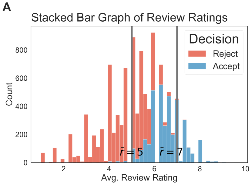
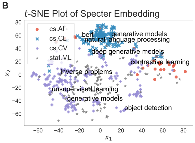
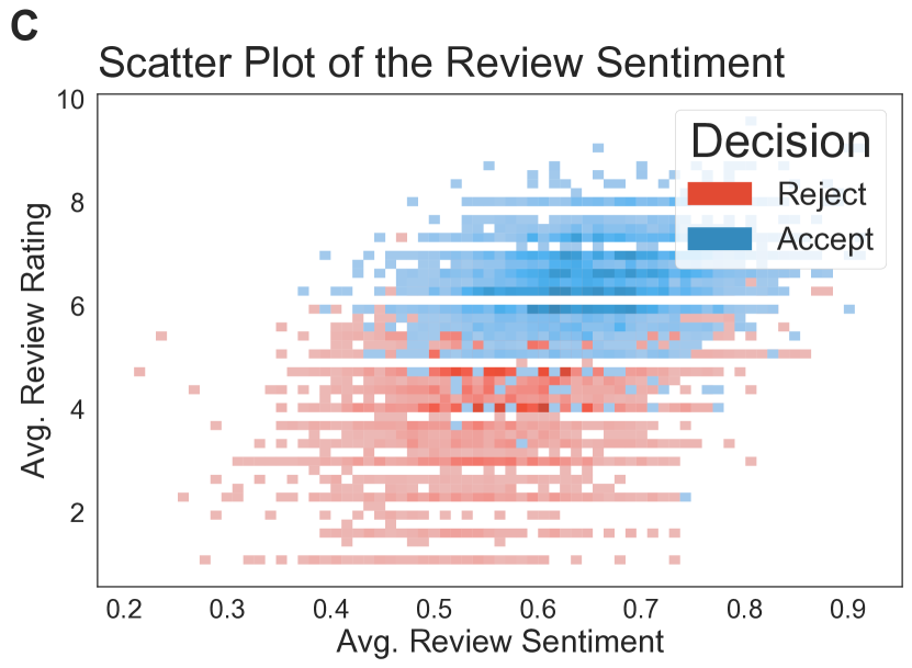
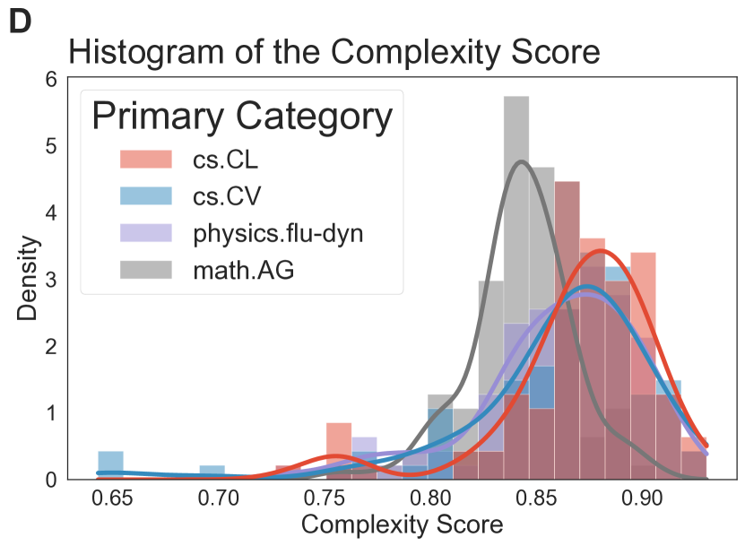
Figure 1: Illustration of ratings and high-level textual features. (A) Stacked bar graphs of acceptance decisions. The decisions of borderline papers (average rating between $5$ and $7$) are not clearcut. (B) $T$-SNE plot of the Specter embedding together with arXiv primary categories and primary keywords among submissions that have been put onto arXiv. (C) Sentiment and ratings of reviews. (D) Distribution of complexity scores of a random samples of arXiv articles across four primary categories.

2.1 Database construction and structural features

We use the ICLR Database collected and complied by Zhang et al., (2022). Motivated by the observation that area chairs’ final decisions of submissions with an average rating between $5$ to $7$ are not deterministic, as shown in Panel A of Figure 1, we restrict ourselves to this subset of borderline submissions. We first briefly recall the data collection and cleaning process here for completeness.

The OpenReview API is used to crawl data of $10,289$ submissions to the International Conference on Learning Representations (ICLR) from $2017$ to $2022$. The crawled data include (i) submissions and their metadata; (ii) author metadata, (iii) review/rebuttal data and (iv) area-chair/program chair decision. Structural features, including the number of sections, figures, tables and bibliographies, are extracted in a relatively straightforward manner. We also extracted and rank self-reported keywords from each submission to form primary and secondary keywords. Author profiles include an optional self-reported gender; we used the first name dictionary developed by Tsai et al., (2016) to provide a numerical score based on the first names of the authors where $0$ signifies female and $1$ otherwise. Author profiles are then augmented via Google Scholar API to obtain author citation and $h$-index data. Author institution is matched using the domain name of the author email. Although CSRanking data is available, it does not have full coverage of all authors’ institutions. As such, we mainly use the institutional ranking derived from the cumulative number of accepted papers to the ICLR in the past. For example, the ranking in 2020 of institution A is determined by all papers accepted to ICLR 2017-2020 that have at least one author from it. The review data include rating, confidence and textual reviews. In some years, for example, 2020 and 2022, there are additional assessments such as technical soundness or novelty. Since these additional assessments are not available for all years, we restrict our attention to ratings, confidence, and higher-level features derived from textual reviews to be discussed shortly. Finally, we dichotomize the paper decision by grouping various acceptance designations (spotlight, poster, short talk) into “Accept” and “Reject” or “invited to workshop track” as “Reject.”

We also identify if a submission has been posted on the preprint platform arXiv.org before the review deadline (i.e., the time reviewers are asked to finalize their reviews) by (i) searching for five most relevant results based on the title and abstract corresponding to each article from arXiv.org, (ii) computing the Jacard similarity and normalized Levenshtein similarity between authors, and (iii) calculating the cosine-similarity of the title-abstract embedding. Using the arXiv timestamp, we then identified which submissions were posted prior to the end of the review process. Among the subset of papers that has arXiv counterparts, we also obtain their arXiv-related metadata such as primary and secondary categories.

2.2 Derived higher-level features

Although the structural features described so far contain abundant information, we considered further leveraging language models to extract additional higher-level features directly from textual data. These higher-level features, like topics, quality of writing and mathematical complexity or rigor, may help quantify residual confounding not captured by structural aspects (e.g., those described in Section 2.1) of an article. Furthermore, in a matched observational study, it is desirable to have a characterization of the “similarity” among study units to serve as a criterion for matching. Therefore, we derived the following higher-level features and a similarity measure based on embeddings from language models to facilitate our study design.

2.2.1 SPECTER Embedding

Our first tool is the SPECTER model (Cohan et al.,, 2020), a BERT-based model (Devlin et al.,, 2019) fine-tuned on a scholarly corpus that has a good track record on summarization tasks (generate abstracts from the main texts) on academic articles. This model takes the abstract of the submissions and outputs a $784$-dimensional real-valued vector as its representation. Panel B of Figure 1 plots a two-dimensional $t$-SNE (van der Maaten and Hinton,, 2008) embedding of this representation across a subset of $535$ submissions that have their arXiv information and primary keyword available. We see that computer vision and computational linguistics articles separate well while general AI and ML articles blend in. In addition, we sample $9$ primary keywords to overlay on the $t$-SNE embedding. Note that semantically similar keywords (e.g., the phrases “BERT” and “natural language processing”) generally have higher proximity under this embedding, which further demonstrate its effectiveness. We thus use this embedding to (1) perform a $10$-component spectral clustering to assign each submission a “semantic cluster” of submissions, and (2) compute the cosine similarity between any two articles.

Sentiment Modeling.

A RoBERTa model (Liu et al.,, 2019) fine-tuned on Twitter sentiments (Rosenthal et al.,, 2017) is used to assign a sentiment score to textual reviews where $0$ signifies negative and $1$ positive. We plot the scatter plot of average sentiment and average rating of submissions with different color signifies different decisions in Panel C of Figure 1. We observe that the sentiment is highly correlated with the rating while behaves more volatile when the rating is borderline. This suggests that incorporating review sentiment may help complement numerical ratings in the downstream analysis, especially when numerical ratings are borderline and not discriminative.

Complexity Score.

We use an off-the-shelf fluency model derived from the RoBERTa model (Liu et al.,, 2019) to assess sentence-level fluency and take the average to represent the complexity of an article, where $1$ signifies most fluent and easy-to-read while $0$ denotes gibberish-like sentences. This fluency score measures how well each article aligns with the English grammar, and serves as a proxy for an article’s heaviness in mathematical notation since in-line mathematical notation often disrupts an English sentence’s fluency and results in a lower score. In Panel D of Figure 1, we perform a sanity-check by randomly sample approximately $100$ arXiv papers from four categories (computational linguistics, computer vision, fluid dynamics, and algebraic geometry) and compute their complexity score. Note that most of the scores are relatively high, as expected since academic articles are often relatively well-written. We also observe a discrepancy in that algebraic geometric papers has its score distribution significantly skewed to the left, which also aligns with our intuition. We thus use this complexity score as a proxy to mathematical complexity and paper readability in our subsequent analysis.

3 Notation and framework

3.1 Matched cohort study

In the absence of a well-controlled experiment (e.g., the hypothetical RCT envisioned in Section 1.2), observational studies, up to their important limitations, provide an alternative to explore a cause-and-effect relationship (Cochran and Chambers,, 1965). In an observational study, study units receiving different levels of treatment may differ systematically in their observed covariates, and this induces the so-called overt bias (Rosenbaum,, 2002, Section 3). In our case study, articles with different author metadata, for instance, those with authors from high-ranking versus relatively lower-ranking academic institutions, could differ systematically in topics, keywords, number of figures and equations, among others, and this would invalidate a naïve comparison.

Statistical matching is a commonly used strategy to adjust for confounding in empirical studies (Rubin,, 1973, 1979; Rosenbaum,, 2002, 2010; Ho et al.,, 2007; Stuart,, 2010). The ultimate goal of statistical matching is to embed non-randomized, observational data into an approximate randomized controlled experiment by designing a matched control (or comparison) group that resembles the treated group in observed pre-treatment covariates by matching on these covariates (Rubin,, 1973, 1979), a balancing score derived from these covariates, e.g., Rosenbaum and Rubin,’s (1983) propensity score, or a combination of both (Rosenbaum and Rubin,, 1985).

We note that there are multiple ways to adjust for observed covariates and draw causal conclusions under the potential outcomes framework, statistical matching being one of them. Other commonly used methods include weighting, modeling the potential outcomes, and a combination of both. We found a matched observational study particularly suited for our case study for three reasons. First, it facilitates testing Fisher’s sharp null hypothesis of no effect, which is an appropriate causal null hypothesis encoding an intriguing notion of fairness, as we will discuss in detail in Section 3.4. Second, a matched design naturally takes into account similarity of textual data (for instance, as measured by cosine similarity based on their embeddings) and is capable of balancing some high-dimensional covariates like keywords in our data analysis. A third strength is mostly stylistic: A matched comparison best resembles Bertrand and Mullainathan,’s (2004) seminal field experiment and is perhaps the easiest-to-digest way to exhibit statistical analysis results to a non-technical audience.

In the rest of this section, we articulate essential elements in our analysis, including study units, treatment to be hypothetically manipulated, potential outcomes, timing of the treatment, pre-treatment variables and causal null hypothesis of interest.

3.2 Study units; treatment and its timing; potential outcomes

As discussed in detail in Greiner and Rubin, (2011), there are two agents in our analysis of the effect of authorship metadata on area chairs’ final decisions: an ICLR article peer-reviewed and having received reviewers’ ratings, and a decision maker, i.e., an area chair or meta reviewer (AC for short), who assigned the final acceptance status to the article. In our analysis, each study unit is a (peer-reviewed ICLR article, area chair) pair. There are a total of $N=10,289$ study units in our compiled database, and $5,313$ of them have three or four reviewers and an average rating between $5$ and $7$ and . We will write the $i$-th study unit as $SU_{i}=(\text{article}_{i},\text{AC}_{i})$.

We define the treatment of interest as an area chair’s perception of a peer-reviewed article’s authorship metadata. This definition is modeled after Bertrand and Mullainathan, (2004) and Greiner and Rubin, (2011) and implies the timing of the treatment: We imagine a hypothetical randomized experiment where peer-reviewed ICLR articles, whose constituent parts include text, tables, figures, reviewers’ ratings and comments, are randomly assigned authorship metadata and presented to the area chair for a final decision. This timing component of the treatment is critical because it implies what are meant to be “pre-treatment variables” under Neyman-Rubin’s causal inference framework, as we will discuss in detail in Section 3.3.

In principle, the most granular author metadata is a complete list of author names with their corresponding academic or research institutions. Let $\vec{A}=\vec{a}$ denote author metadata and $\mathcal{A}$ the set of all possible configurations of author metadata. There is one potential outcome $Y_{i}(\vec{a})$ associated with unit $i$ and each $\vec{a}\in\mathcal{A}$; in words, there is one final decision associated with each peer-reviewed article had the author metadata been $\vec{a}$. We will assume the consistency assumption so that the observed outcome $Y_{i}^{\textsf{obs}}=Y_{i}(\vec{a}^{\text{obs}})$. One may adopt a variant of the Stable Unit Treatment Value Assumption or SUTVA (Rubin,, 1980) to reduce the number of potential outcomes. For instance, one may further assume that the potential outcome $Y_{i}(\vec{a})$ depends on author metadata $\vec{a}$ only via authors’ academic institutions. Let $f(\cdot)$ denote a mapping from author metadata to authors’ academic institutions, then this “stability” assumption amounts to assuming $Y_{i}(\vec{a})=Y_{i}(\vec{a}^{\prime})$ when $f(\vec{a})=f(\vec{a}^{\prime})$. We do not a priori make such stability assumptions.

Example 1 (Field experiment in Bertrand and Mullainathan, (2004)).

In Bertrand and Mullainathan,’s (2004) field experiment, each study unit consists of a resume $i$ and a human resource person reading the resume $i$, i.e., $SU_{i}=(\text{resume}_{i},\text{HR person}_{i})$. Treatment is a person’s perception of the name on the resume. In this case, $\mathcal{A}$ would consist of all names and $Y_{i}(A=a)$ is the potential administrative decision had the resume $i$ been associated with name $a$. If we further make the stability assumption that $Y_{i}(a)$ depends on $a$ only via its race and ethnicity connotation as in Bertrand and Mullainathan, (2004) and define $f(a)=1$ if the name $a$ is African-American sounding and $0$ if it is White sounding, then the set of potential outcomes $Y_{i}(a),~{}a\in\mathcal{A}$ would reduce to $\{Y_{i}(1),Y_{i}(0)\}$.

3.3 Observed and unobserved pre-treatment variables

According to Rubin, (2005), covariates refer to “variables that take their values before the treatment assignment or, more generally, simply cannot be affected by the treatment.” Below, we briefly review a dichotomy of pre-treatment variables in the context of drawing causal conclusions from textual data (Zhang and Zhang,, 2022).

In human populations research, pre-treatment variables or covariates are often divided into two broad categories: observed and unobserved; see, e.g., Rosenbaum, (2002, 2010). A randomized controlled experiment like the one in Bertrand and Mullainathan, (2004) had the key advantage of balancing both observed and unobserved confounding, while drawing causal conclusions from observational data inevitably suffers from the concern of unmeasured confounding and researchers often control for a large number of observed covariates in order to alleviate this concern.

When study units are textual data, Zhang and Zhang, (2022) divides observed covariates into two types: explicit observed covariates $\bf X^{\textsf{exp}}_{\textsf{obs}}$ that could be derived from textual data at face value, e.g., number of equations, tables and illustrations in the article, and implicit observed covariates $\bf X^{\textsf{imp}}_{\textsf{obs}}$ that capture higher-level aspects of textual data, e.g., the topic, flow and novelty of the article. In our case study, we will consider the following explicit observed covariates: year of submission, reviewers’ ratings, number of authors, sections, figures and reference, and keywords. We further extracted each article’s complexity, topic and reviewers’ sentiment using state-of-the-art, natural language processing models as described in Section 2.

Unmeasured confounding is a major concern for any attempt to draw a cause-and-effect conclusion from observational data, regardless of the covariance adjustment method. Despite researchers’ best intention and effort to control for all relevant pre-treatment variables via matching, there is always a concern about unmeasured confounding bias as we are working with observational data. In our analysis of ICLR papers, we identified two sources of unmeasured confounding. First, there could be residual confounding due to the insufficiency of language models (such as the SPECTER model) in summarizing or extracting implicit observed covariates $\bf X^{\textsf{imp}}_{\textsf{obs}}$ like topics, flow and sentiment. Second, in our analysis, we used numeric ratings from reviewers as a proxy of the quality and novelty of the article. Reviewers’ ratings may not be sufficient in summarizing the quality of the articles. Unmeasured confounding may lead to a spurious causal conclusion and researchers routinely examine the robustness of the putative causal conclusion using a sensitivity analysis (see, e.g., Rosenbaum,, 2002, 2010; VanderWeele and Ding,, 2017, among many others).

3.4 Causal null hypothesis: A case for Fisher

A causal statement is necessarily a comparison among potential outcomes. In the context of a many-level treatment assignment, Fisher’s sharp null hypothesis states the following:

$$H_{0,\text{sharp}}\mathrel{\mathop{\ordinarycolon}}\quad Y_{i}(\vec{a})=Y_{i}(\vec{a}^{\prime}),\quad\forall i=1,\dots,N~{}\text{and}~{}\vec{a},\vec{a}^{\prime}\in\mathcal{A}.$$ (1)

Fisher’s sharp null hypothesis prescribes a notion of fairness that, arguably, best suits our vision: area chairs’ final decisions of the articles are irrelevant of author metadata; in other words, the decision $Y_{i}(\vec{a})$ could potentially depend on any substantive aspect of the article $i$, including its topic, quality of writing, reviewers’ ratings, etc, but would remain the same had we changed author metadata from $\vec{a}$ to $\vec{a}^{\prime}$.

In addition to Fisher’s sharp null hypothesis, Neyman’s weak null hypothesis, which states that the sample average treatment effect is zero, is another commonly tested causal null hypothesis. Unlike Fisher’s sharp null, Neyman’s weak null hypothesis allows perception bias of varying magnitude for all article-AC pairs, as long as these biases would cancel out each other in one way or another. We found this a sub-optimal notion of fairness compared to that encoded by Fisher’s sharp null hypothesis, and we will focus on testing Fisher’s sharp null hypothesis in our data analysis.

Example 2 (continues=ex:Field experiment).

Bertrand and Mullainathan, (2004) found that White sounding names receive $50$ percent more callbacks for interviews; under the stability assumption discussed in Section 3.2, their findings could be interpreted as a causal effect of perceiving White versus African-American sounding names. In the absence of the stability assumption, Bertrand and Mullainathan,’s result could still be interpreted as providing evidence against Fisher’s sharp null hypothesis $H_{0,\text{sharp}}$ in its most generic form, although in what specific ways $H_{0,\text{sharp}}$ is violated needs further investigation.

Unlike Bertrand and Mullainathan,’s (2004) randomized experiment that randomly assigns resume names, our cohort of ICLR articles are not randomly assigned authorship metadata. It is conceivable that articles with more “prestigious” authors, however one might want to define the concept of “prestige,” could differ systematically in their reviewers’ ratings, topics, etc, and this difference in baseline covariates could potentially introduce a spurious association between author metadata and area chairs’ final decisions. To overcome this, we embed the observational data into a matched-pair design by constructing $I$ matched pairs, each with two peer-reviewed articles, indexed by $j=1,2$, such that these two articles are as similar as possible in their covariates but with different author metadata. Let $\vec{a}_{ij}$ denote the author metadata associated with article $j$ in the matched pair $i$. Such a matched-pair design enables us to test the following sharp null hypothesis:

$$H^{\prime}_{0,\text{sharp}}\mathrel{\mathop{\ordinarycolon}}\quad Y_{ij}(\vec{a}_{i1})=Y_{ij}(\vec{a}_{i2}),\quad\forall i=1,\dots,I,~{}j=1,2.$$ (2)

We note that $H_{0,\text{sharp}}$ in (1) implies $H^{\prime}_{0,\text{sharp}}$ in (2), so rejecting $H^{\prime}_{0,\text{sharp}}$ would then provide evidence against $H_{0,\text{sharp}}$. Such a design is termed “near-far” design in the literature (Baiocchi et al.,, 2010, 2012) and has been used in a number of empirical studies (see, e.g., Lorch et al.,, 2012; Neuman et al.,, 2014; MacKay et al.,, 2021, among others).

4 Data analysis: study design and outcome analysis

4.1 A first matched comparison: design M1

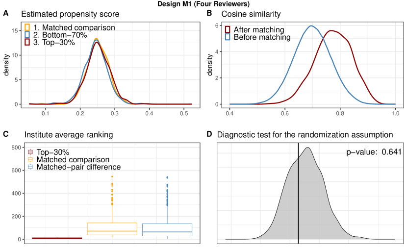
Figure 5: Diagnostics of design M1. Panel A: Estimated propensity score top-30% articles, bottom-70% articles and matched comparison articles. Panel B: Distribution of between-article cosine similarity before (median = 0.70) and after matching (median = 0.78). Panel C: Boxplots of authors’ average institution rankings and matched-pair differences in authors’ average institution rankings. The average, within-matched-pair difference in the institution ranking is 99.6 among 602 matched pairs in this stratum (median: 63.5; interquartile range 28.5-135.0). Panel D: Permutation distribution and the observed test statistic of the classification permutation test.

We restricted our attention to $5,313$ borderline articles that were peer-reviewed by $3$ or $4$ reviewers and received an average rating between $5$ and $7$. We first considered a study design M1 where each matched pair consisted of one article whose authors’ average institution ranking was among the top $30\%$ of these $5,313$ submissions and the other article whose authors’ average institution ranking was among the bottom $70\%$. Columns 2 and 3 of Table 1 summarize the characteristics, including structural features and derived higher-level features, of $1,585$ top-$30\%$ articles and those of the other $3,728$ articles. As one closely examines these two columns, a number of features, including submission year, number of figures, complexity score as judged by the language model, keyword and topic, differ systematically among these submissions. Matching helps remove most of the overt bias: In the matched comparison group (which is a subset of size $n=1,585$ from the reservoir of $3,728$ articles), standardized mean differences of all but one covariates are less than $0.1$, or one-tenth of one pooled standard deviation. In fact, design M1 required near-exact matching on important covariates like reviewers’ ratings and year of submission, and achieved near-fine balance for categorical variables like topic cluster and primary keyword (Rosenbaum et al.,, 2007). Algorithms used to construct the matched design M1 will be described in detail in Section 4.3. Panel C in Figure 2 assesses how different two articles in each matched pair are in their authors’ average institution rankings; see Figure 5 in Appendix for similar plots in the four-reviewer stratum. The average, within-matched-pair difference in authors’ average institution ranking is $74.3$ among $983$ matched pairs in the three-reviewer stratum (median: $49.6$; interquartile range $26.6$-$96.7$) and $99.6$ among $602$ matched pairs in the four-reviewer stratum (median: $63.5$; interquartile range $28.5$-$135.0$). We concluded that there was a sizable difference in author metadata between two articles in each matched pair.

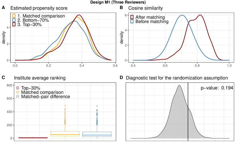
Figure 2: Diagnostics of design M1. Panel A: Estimated propensity score top-30% articles, bottom-70% articles and matched comparison articles. Panel B: Distribution of between-article cosine similarity before (median = 0.71) and after matching (median = 0.80). Panel C: Boxplots of authors’ average institution rankings and matched-pair differences in authors’ average institution rankings. Panel D: Permutation distribution and the observed test statistic of the classification permutation test.

Table 1: Characteristics of articles before and after matching in the design M1.

[h] Bottom $70\%$ Ranking Articles (n = 3,728) Top $30\%$ Ranking Articles (n = 1,585) SMD (Before Matching) Matched Comparison Articles (n = 1,585) SMD (After Matching) Conference and Reviewer Year of submission (%)        2017 109 ( 2.9) 129 ( 8.1) 0.23 92 ( 5.8) 0.10        2018 299 ( 8.0) 221 (13.9) 0.19 201 (12.7) 0.04        2019 520 (13.9) 303 (19.1) 0.14 304 (19.2) $<0.01$        2020 548 (14.7) 231 (14.6) 0.003 234 (14.8) $<0.01$        2021 1200 (32.2) 388 (24.5) 0.171 412 (26.0) 0.03        2022 1052 (28.2) 313 (19.7) 0.2 342 (21.6) 0.05 Reviewer Ratings        Reviewer I 6.99 (0.92) 6.99 (0.91) 0.008 6.97 (0.90) 0.02        Reviewer II 6.12 (0.80) 6.12 (0.79) 0.001 6.12 (0.78) $<0.01$        Reviewer III 5.21 (1.08) 5.18 (1.09) 0.031 5.19 (1.10) 0.01        Reviewer IV* 4.71 (1.06) 4.74 (1.11) 0.031 4.74 (1.09) $<0.01$ Reviewer Sentiment        Reviewer I 0.75 (0.10) 0.75 (0.11) 0.026 0.75 (0.11) 0.03        Reviewer II 0.64 (0.09) 0.64 (0.09) 0.021 0.64 (0.09) 0.04        Reviewer III 0.55 (0.10) 0.54 (0.10) 0.081 0.54 (0.10) 0.01        Reviewer IV* 0.49 (0.09) 0.50 (0.09) 0.062 0.50 (0.09) 0.01 Article Metadata No. Author 4.21 (1.67) 4.17 (1.69) 0.024 4.13 (1.67) 0.03 No. Figure 13.71 (7.26) 12.55 (7.55) 0.156 12.42 (6.60) 0.02 No. Reference 42.53 (16.59) 42.19 (16.93) 0.020 40.98 (14.94) 0.07 No. Section 19.94 (7.16) 19.96 (7.11) 0.003 19.74 (6.90) 0.03 Complexity, Topics and Keywords Complexity 0.84 (0.03) 0.85 (0.03) 0.285 0.85 (0.03) 0.06 Topic cluster^† (%)         RL/Meta Learning/Robustness 367 ( 9.8) 113 ( 7.1) 0.097 113 ( 7.1) 0         RL/CV/Robustness 298 ( 8.0) 80 ( 5.0) 0.122 80 ( 5.0) 0         DL/GM/CNN 345 ( 9.3) 147 ( 9.3) 0 147 ( 9.3) 0         DL/RNN/GNN 365 ( 9.8) 133 ( 8.4) 0.049 133 ( 8.4) 0         DL/Optimization/Generalization 399 (10.7) 126 ( 7.9) 0.097 126 ( 7.9) 0         DL/Robustness/Adversarial Examples 445 (11.9) 270 (17.0) 0.145 270 (17.0) 0         DL/RL/Unsupervised Learning/GM 319 ( 8.6) 143 ( 9.0) 0.014 143 ( 9.0) 0         DL/Multi-Agent or Model-Based RL/IL 475 (12.7) 209 (13.2) 0.015 209 (13.2) 0         DL/Federated or Distributed Learning 370 ( 9.9) 260 (16.4) 0.193 260 (16.4) 0         GM/GAN/VAE 345 ( 9.3) 104 ( 6.6) 0.1 104 ( 6.6) 0 Primary keyword (%)        NA 950 (25.5) 347 (21.9) 0.085 368 (23.2) 0.03        Other 794 (21.3) 292 (18.4) 0.073 312 (19.7) 0.03        Deep learning 393 (10.5) 242 (15.3) 0.144 238 (15.0) 0.01        Reinforcement learning 290 ( 7.8) 183 (11.5) 0.126 181 (11.4) $<0.01$        Graph neural networks 145 ( 3.9) 41 ( 2.6) 0.073 39 ( 2.5) $<0.01$        Representation learning 109 ( 2.9) 40 ( 2.5) 0.025 39 ( 2.5) $<0.01$        Generative models 89 ( 2.4) 35 ( 2.2) 0.013 38 ( 2.4) 0.01        Meta-learning 79 ( 2.1) 34 ( 2.1) 0 33 ( 2.1) $<0.01$        Self-supervised learning 72 ( 1.9) 23 ( 1.5) 0.031 24 ( 1.5) $<0.01$        Unsupervised learning 70 ( 1.9) 43 ( 2.7) 0.053 32 ( 2.0) 0.05        Neural networks 62 ( 1.7) 30 ( 1.9) 0.015 25 ( 1.6) 0.02        Generative adversarial networks 56 ( 1.5) 14 ( 0.9) 0.055 18 ( 1.1) 0.02        Optimization 43 ( 1.2) 26 ( 1.6) 0.034 26 ( 1.6) 0        Variational inference 39 ( 1.0) 8 ( 0.5) 0.058 11 ( 0.7) 0.02        Transformer 37 ( 1.0) 20 ( 1.3) 0.028 15 ( 0.9) 0.04        Generalization 36 ( 1.0) 32 ( 2.0) 0.082 22 ( 1.4) 0.05 Decision Acceptance (%) 1928 ( 51.7) 811 ( 51.2) 851 ( 53.7)

• Reviewer IV’s rating and sentiment results are derived from articles within the stratum of four reviewers.

• RL: Reinforcement Learning; GM: Generative Models; CV: Computer Vision; CNN: Convolutional Neural Nets; RNN: Recurrent Neural Nets; GNN: Graph Neural Nets; IL: Imitation Learning; GAN: Generative Adversarial Nets; VAE: Variational Auto-Encoder. Note that the description is not exhaustive.

To further demonstrate two groups are well comparable, Panel A of Figure 2 displays the distribution of the estimated “propensity score,” defined as the probability that authors’ average ranking of an article was among top $30\%$, in each of the following three groups: top-30% articles (red), bottom-70% articles (blue), and matched comparison articles (yellow), all in the three-reviewer stratum. Similar plots for articles with four reviewers can be found in Appendix. As is evident from the figure, the propensity score distribution of the matched comparison articles is more similar to that of the top-30% articles. Panel B of Figure 2 further plots the cosine similarity calculated from the raw textual data of each article. It is also evident that two articles in the same matched pair now have improved cosine similarity compared to that from two randomly drawn articles prior to matching. Our designed matched comparison M1 appears to be well balanced in many observed covariates and resembles a hypothetical RCT where we randomly assign author metadata.

The question remains as to whether the balance is sufficiently good compared to an authentic RCT and could justify randomization inference. We conducted a formal diagnostic test using Gagnon-Bartsch and Shem-Tov,’s (2019) classification permutation test (CPT) based on random forests to test the randomization assumption for the matched cohort. The randomization assumption cannot be rejected in either the three-reviewer or four-reviewer stratum (p-value = $0.194$ and $0.641$, respectively); see the null distribution and test statistic in Panel D of Figure 2 and Figure 5 in Appendix.

Table 2: Contingency table, p-values (exact, two-sided McNemar’s test) and odds ratio (Fay,, 2010) of $1,585$ matched pairs in the design M1 and $1051$ matched pairs in a strengthened design M2. Defining and interpreting the odds ratio and its confidence interval requires an additional “stability” assumption discussed in Section 3.2.

Panel A: Design M1		Comparison Articles			Odds Ratio
		Accepted	Rejected	P-value	95% CI
Top-30% Articles	Accepted	633	178	0.050	0.82
	Rejected	218	556		[0.67, 1.00]
Panel B: Design M2		Comparison Articles
		Accepted	Rejected
Top-30% Articles	Accepted	443	115	0.149	0.83
	Rejected	139	354		[0.64, 1.07]

Panel A of Table 2 summarizes the outcomes of $1,585$ matched pairs of two articles. We tested Fisher’s sharp null hypothesis $H^{\prime}_{0,\text{sharp}}$ reviewed and discussed in Section 3.4 using a two-sided, exact McNemar’s test (Fay,, 2010) and obtained a p-value of $0.050$, which suggested some weak evidence that authorship metadata was associated with AC’s final decisions. Under an additional stability assumption stating that the potential acceptance status $Y(\vec{a})$ depended on author metadata $\vec{a}$ only via authors’ average institution ranking and remained unchanged when the average ranking is among the top-30% or among the bottom-70%, we estimated the odds ratio to be $0.82$ (95% CI: [0.67, 1.00]), providing some weak evidence that borderline articles from top-30% institutions were less favored by area chairs compared to their counterparts from the comparison group. Note that a naïve, unadjusted comparison between the top-30% and bottom-70% borderline articles would in fact mask any difference (acceptance rate: 51.2% versus 51.7% before matching).

Our analysis seems to defy the common wisdom that there is a “status bias” favoring higher-profile authors. It is then natural to ask, if author metadata were even more drastically different, shall we then see some evidence for status bias that would better align with previous findings? This inquiry led to a second, strengthened design M2.

4.2 A strengthened design M2

Baiocchi et al., (2010) first considered “strengthening” an encouragement variable (differential distance) in the context of an instrumental variable analysis of the effect of low-level versus high-level neonatal intensive care units (NICUs) on mortality rate. In their analysis, Baiocchi et al., (2010) compared mothers who lived near to and far from a high-level NICU and “strengthened” the comparison by restricting their analysis to a smaller subset of comparable mothers who lived very near to and very far from a high-level NICU. We adopted their idea here and constructed a strengthened design M2 where one article in each matched pair is a top-20% article (as opposed to a top-30% article in design M1) and the other matched comparison article was from the reservoir of bottom-80% articles. We also added a “dose-caliper” in the statistical matching algorithm to further separate the average ranking within each matched pair; see Section 4.3 for details.

A total of $1,051$ matched pairs were formed. Panel C of Figure 3 summarizes the within-matched-pair difference in authors’ average institution ranking across $1,051$ matched pairs in the strengthened design M2. In this strengthened design, the average difference now increases from $74.3$ (as in the design M1) to $108.8$. Importantly, the cohort of top-20% articles and their matched comparison group are still comparable in all baseline covariates, as summarized in Table 3. Similar to the design M1, we cannot reject the randomization assumption based on the classification permutation test (p-value = $0.961$).

Panel B of Table 2 summarizes the outcomes of $1,051$ matched pairs of two articles in the strengthened design M2. Under the additional stability assumption, we obtained a near identical point estimate for odds ratio (OR = $0.83$ in M2 versus $0.82$ in M1), though the estimate is slightly less precise as a result of a smaller sample size ($1,051$ in M2 versus $1,585$ in M1). Consistent results across two study designs help reinforce the conclusion that we did not find evidence supporting a “status bias” favoring authors from high-ranking institutions in this cohort of borderline articles.

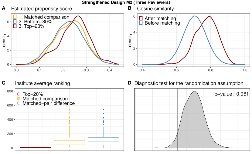
Figure 3: Diagnostics of design M2. Panel A: Estimated propensity score top-30% articles, bottom-70% articles and matched comparison articles. Panel B: Distribution of between-article cosine similarity before (median = 0.71) and after matching (median = 0.78). Panel C: Boxplots of authors’ average institution rankings and matched-pair differences in authors’ average institution rankings. Panel D: Permutation distribution and the observed test statistic of the classification permutation test.

Table 3: Characteristics of articles before and after matching in a strengthened design M2.

[h] All Control Articles (n = 4,262) All Treated Articles (n = 1,051) SMD (Before Matching) Matched Control Articles (n = 1,051) SMD (After Matching) Conference and Reviewer Year of submission (%)        2017 144 ( 3.4) 94 ( 8.9) 0.23 77 ( 7.3) 0.07        2018 380 ( 8.9) 140 (13.3) 0.14 126 (12.0) 0.04        2019 614 (14.4) 209 (19.9) 0.146 201 (19.1) 0.02        2020 621 (14.6) 158 (15.0) 0.011 157 (14.9) $<0.01$        2021 1343 (31.5) 245 (23.3) 0.185 272 (25.9) 0.06        2022 1160 (27.2) 205 (19.5) 0.183 218 (20.7) 0.03 Reviewer Ratings        Reviewer I 6.98 (0.92) 7.04 (0.91) 0.059 7.01 (0.89) 0.02        Reviewer II 6.12 (0.79) 6.13 (0.79) 0.017 6.11 (0.78) 0.03        Reviewer III 5.21 (1.07) 5.16 (1.11) 0.042 5.17 (1.09) $<0.01$        Reviewer IV* 4.71 (1.06) 4.77 (1.12) 0.052 4.74 (1.13) 0.02 Reviewer Sentiment        Reviewer I 0.75 (0.10) 0.76 (0.11) 0.051 0.75 (0.10) 0.10        Reviewer II 0.64 (0.09) 0.64 (0.09) 0.005 0.64 (0.09) 0.08        Reviewer III 0.55 (0.10) 0.54 (0.10) 0.062 0.54 (0.10) 0.03        Reviewer IV* 0.49 (0.09) 0.50 (0.09) 0.120 393 0.06 Article Metadata No. uthor 4.21 (1.67) 4.17 (1.72) 0.023 4.19 (1.66) 0.01 No. Figure 13.60 (7.41) 12.41 (7.10) 0.164 12.32 (6.45) 0.01 No. Reference 42.56 (16.61) 41.91 (17.02) 0.039 40.50 (15.12) 0.08 No. Section 19.94 (7.16) 19.96 (7.06) 0.003 19.54 (6.94) 0.06 Complexity, Topics and Keywords Complexity 0.84 (0.03) 0.85 (0.03) 0.308 0.85 (0.03) 0.15 Topic cluster ^† (%)         RL/Meta Learning/Robustness 404 ( 9.5) 76 ( 7.2) 0.083 76 ( 7.2) 0         RL/CV/Robustness 328 ( 7.7) 50 ( 4.8) 0.12 50 ( 4.8) 0         DL/GM/CNN 393 ( 9.2) 99 ( 9.4) 0.007 99 ( 9.4) 0         DL/RNN/GNN 408 ( 9.6) 90 ( 8.6) 0.035 90 ( 8.6) 0         DL/Optimization/Generalization 439 (10.3) 86 ( 8.2) 0.073 86 ( 8.2) 0         DL/Robustness/Adversarial Examples 551 (12.9) 164 (15.6) 0.077 164 (15.6) 0         DL/RL/Unsupervised Learning/GM 365 ( 8.6) 97 ( 9.2) 0.021 97 ( 9.2) 0         DL/Multi-Agent or Model-Based RL/IL 545 (12.8) 139 (13.2) 0.012 139 (13.2) 0         DL/Federated or Distributed Learning 435 (10.2) 195 (18.6) 0.241 195 (18.6) 0         GM/GAN/VAE 394 ( 9.2) 55 ( 5.2) 0.155 55 ( 5.2) 0 Primary keyword (%)        NA 1084 (25.4) 213 (20.3) 0.122 220 (20.9) 0.01        Other 891 (20.9) 195 (18.6) 0.058 195 (18.6) 0        Deep learning 460 (10.8) 175 (16.7) 0.172 178 (16.9) $<0.01$        Reinforcement learning 353 ( 8.3) 120 (11.4) 0.104 122 (11.6) $<0.01$        Graph neural networks 162 ( 3.8) 24 ( 2.3) 0.087 24 ( 2.3) 0        Representation learning 127 ( 3.0) 22 ( 2.1) 0.057 22 ( 2.1) 0        Generative models 99 ( 2.3) 25 ( 2.4) 0.007 26 ( 2.5) $<0.01$        Meta-learning 89 ( 2.1) 24 ( 2.3) 0.014 23 ( 2.2) $<0.01$        Self-supervised learning 80 ( 1.9) 15 ( 1.4) 0.039 14 ( 1.3) $<0.01$        Unsupervised learning 79 ( 1.9) 34 ( 3.2) 0.083 26 ( 2.5) 0.04        Neural networks 73 ( 1.7) 19 ( 1.8) 0.008 17 ( 1.6) 0.02        Generative adversarial networks 62 ( 1.5) 8 ( 0.8) 0.066 10 ( 1.0) 0.02        Generalization 48 ( 1.1) 20 ( 1.9) 0.066 16 ( 1.5) 0.03        Optimization 47 ( 1.1) 22 ( 2.1) 0.08 22 ( 2.1) 0        Variational inference 44 ( 1.0) 3 ( 0.3) 0.087 7 ( 0.7) 0.05 Decision Acceptance (%) 2181 ( 51.2) 558 ( 53.1) 582 ( 55.4)

• Reviewer IV’s rating and sentiment results are derived from articles within the stratum of four reviewers.

• RL: Reinforcement Learning; GM: Generative Models; CV: Computer Vision; CNN: Convolutional Neural Nets; RNN: Recurrent Neural Nets; GNN: Graph Neural Nets; IL: Imitation Learning; GAN: Generative Adversarial Nets; VAE: Variational Auto-Encoder. Note that the description is not exhaustive.

4.3 Matching algorithm: matching one sample according to multiple criteria

The matched sample M1 displayed in Table 1 was constructed using an efficient, network-flow-based optimization algorithm built upon a tripartite network (Zhang et al.,, 2021) as opposed to a traditional, bipartite network (Rosenbaum,, 1989). Compared to a bipartite network, a tripartite network structure helps separate two tasks in the design of an observational study: (1) constructing closely matched pairs and (2) constructing a well balanced matched sample. A detailed account of the algorithm can be found in Zhang et al., (2021); below, we described how we designed the cost in the tripartite network and achieved the features of M1 and M2 described in Section 4.1 and 4.2.

Figure 4: An illustrative plot of a tripartite network consisting of three treated units and five candidate control units.

Figure 4 illustrates the basic tripartite network structure with three units, $\{\gamma_{1},\gamma_{2},\gamma_{3}\}$, from the top-30% articles and five units, $\{\tau_{1},\dots,\tau_{5}\}$, from the reservoir of bottom-70% articles. To run a tripartite-network-based matching algorithm, two costs need to be specified (Zhang et al.,, 2021). The cost $\delta_{\gamma_{i},\tau_{j}}$ associated with each edge $e$ connecting $\gamma_{i}$ and $\tau_{j}$ in the left part of the network encodes criteria for closely matched pairs. To construct the matched sample M1, we let $\delta_{\gamma_{i},\tau_{j}}$ be the cosine similarity derived from the SPECTER embeddings of article $\gamma_{i}$ and $\tau_{j}$. We then enforce near-exact matching on submission year and reviewers’ ratings by adding a large penalty to $\delta_{\gamma_{i},\tau_{j}}$ if articles $\gamma_{i}$ and $\tau_{j}$ were submitted to the ICLR conference in different calendar years or did not receive same ratings. As a result, two articles in each matched pair were exactly or near-exactly matched on reviewers’ ratings. For instance, a top-30% article $\gamma_{i}$ submitted at $2017$ and peer-reviewed by three reviewers and received ratings of $6$, $5$ and $5$ (from highest to lowest) was matched to a $2017$-submitted, $(6,5,5)$-rated bottom-70% article $\tau_{j}$. This conscious design of $\delta_{\gamma_{i},\tau_{j}}$ helped achieve improved within-matched-pair cosine similarity and near-exact match on year of submission and reviewers’ ratings in M1.

The cost $\Delta_{\overline{\gamma}_{i},\overline{\tau}_{j}}$ associated with edge connecting $\overline{\gamma}_{i}$ and $\overline{\tau}_{j}$ in the right part of the network encodes criteria for good overall balance when groups are viewed as a whole. To construct M1, we estimated the propensity score based on article metadata and set $\Delta_{\overline{\gamma}_{i},\overline{\tau}_{j}}$ to be the difference in the estimated propensity score to minimize earth-mover’s distance between the propensity score distributions of the top-30% articles and their matched comparison articles. The “balancing” property of the propensity score (Rosenbaum and Rubin,, 1983) then helped balance the covariates used to estimate it. One limitation of the propensity score is that its stochastic balancing property often does not suffice when balancing nominal variables with many categories; in these scenarios, a design technique known as fine balance is often used in conjunction with propensity score matching (Rosenbaum et al.,, 2007; Rosenbaum,, 2010). In short, fine balance is a technique that forces the frequency of one or more nominal variables to be identical or as close as possible in two groups. We finely balanced the topic clusters and keywords by adding a large penalty to $\Delta_{\overline{\gamma}_{i},\overline{\tau}_{j}}$ when $\gamma_{i}$ and $\tau_{j}$ differed in the topic cluster or keyword. Finally, matched pairs in M1 were obtained as a result of solving the minimum-cost flow optimization problem associated with this tripartite network. We conducted matching in the stratum of articles with three reviewers and four reviewers, respectively, because articles in the four-reviewer stratum have two additional covariates: a fourth reviewer rating and a fourth reviewer sentiment.

Our construction of the design M2 was analogous to that of M1, except that we further added a “dose-caliper,” defined as a large penalty when two articles $\gamma_{i}$ and $\tau_{j}$ differ in their authors’ average institution rankings by less than a pre-specified caliper size, to the cost $\delta_{\gamma_{i},\tau_{j}}$. The average within-matched-pair difference in authors’ average rankings is $74.3$ in M1; hence, we set the caliper size to be $80$ when constructing M2. In this way, the within-matched-pair difference in authors’ average ranking was as large as $108.8$ in the design M2, representing a meaningful improvement over that in M1.

5 Discussion: interpretation of our results; limitations

In this article, we studied the association between author metadata and area chairs’ decisions. We did not find evidence supporting a status bias, that is, area chairs’ decisions systematically favored authors from high-ranking institutions, when comparing two cohorts of borderline articles with near-identical reviewers’ ratings, sentiment, topics, primary keywords and article metadata. Under an additional stability assumption, we found that articles from high-ranking institutions had a lower acceptance rate and the result was consistent among articles from top-30% institutions (odds ratio = $0.82$) and top-20% institutions (odds ratio = $0.83$).

Our results need to be interpreted under an appropriate context. First, like all retrospective, observational studies, although we formulated the question under a rigorous causal framework, we cannot be certain that our analysis was immune from any unmeasured confounding bias. For instance, the marginally higher acceptance rate of articles in the matched comparison groups (i.e., articles from lower-ranking institutions) could be easily explained away if these articles, despite having near-identical reviewers’ ratings as their counterparts in the top-30% or top-20% groups, were in fact superior in their novelty and significance and area chairs made decisions based on these attributes rather than author metadata.

Second, any interpretation of our results should be restricted to our designed matched sample and should not be generalized to other contexts. In particular, we only focused on area chairs’ decision on borderline articles. As Greiner and Rubin, (2011, Section III) articulated in great detail, a study unit may interact with multiple agents of an overall system and we have more than one choice of decider to study. In our case study, an ICLR article has interacted with at least two types of deciders, a group of reviewers and an area chair. We explicitly focused on the interaction between a peer-reviewed article and an area chair. This deliberate choice allowed us to control for some valuable pre-treatment variables, including reviewers’ ratings and sentiment, that are good proxies for articles’ innate quality; however, by choosing to focus on this interaction that happened after the interaction between an article and multiple reviewers, we forwent the opportunity to detect any status bias, in either direction, in any earlier interaction including the peer review process that could have affected the values of pre-treatment variables in our analysis (Greiner and Rubin,, 2011). Although the peer-review process of ICLR is in principle double-blind, it is conceivable that articles’ author metadata could be leaked (e.g., when articles were posted in the pre-print platform) during the peer review process, and reviewers’ ratings could be biased in favor of more (or less) established authors. It is of great interest to further study any perception bias during the interaction between articles and their reviewers; however, a key complication facing such an analysis is that articles may not be comparable without having a relatively objective judgment or rating (e.g., reviewers’ ratings in our analysis of area chairs’ decision).

With all these important caveats and limitations in mind, we found our analysis a solid contribution to the social science literature on status bias. Our analysis also helps clarify many important causal inference concepts and misconceptions when study units are textual data, including (1) the importance of shifting focus from an attribute to the perception of it, (2) the importance of articulating the timing of the treatment and hence what constitutes pre-treatment variables, (3) Fisher’s sharp null hypothesis as a relevant causal null hypothesis in the context of fairness, and (4) Rubin,’s (1980) stability assumption often implicitly assumed but overlooked, all within a concrete case study.

Appendix

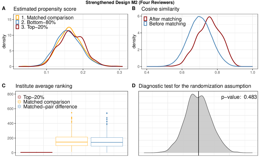
Figure 6: Diagnostics of design M2. Panel A: Estimated propensity score top-30% articles, bottom-70% articles and matched comparison articles. Panel B: Distribution of between-article cosine similarity before (median = 0.70) and after matching (median = 0.76). Panel C: Boxplots of authors’ average institution rankings and matched-pair differences in authors’ average institution rankings. The average, within-matched-pair difference in the institution ranking is 162.5 among 393 matched pairs in this stratum (median: 144.6; interquartile range 90.2-208.0). Panel D: Permutation distribution and the observed test statistic of the classification permutation test.

References

- Baiocchi et al., (2010) Baiocchi, M., Small, D. S., Lorch, S., and Rosenbaum, P. R. (2010). Building a stronger instrument in an observational study of perinatal care for premature infants. Journal of the American Statistical Association, 105(492):1285–1296.
- Baiocchi et al., (2012) Baiocchi, M., Small, D. S., Yang, L., Polsky, D., and Groeneveld, P. W. (2012). Near/far matching: a study design approach to instrumental variables. Health Services and Outcomes Research Methodology, 12(4):237–253.