Sublinear Time Algorithms and Complexity of Approximate Maximum Matching
Abstract
Sublinear time algorithms for approximating maximum matching size have long been studied. Much of the progress over the last two decades on this problem has been on the algorithmic side. For instance, an algorithm of Behnezhad [5] obtains a 1/2-approximation in time for -vertex graphs. A more recent algorithm by Behnezhad, Roghani, Rubinstein, and Saberi [8] obtains a slightly-better-than-1/2 approximation in time (for arbitrarily small constant ). On the lower bound side, Parnas and Ron [22] showed 15 years ago that obtaining any constant approximation of maximum matching size requires time. Proving any super-linear in lower bound, even for -approximations, has remained elusive since then.
In this paper, we prove the first super-linear in lower bound for this problem. We show that at least queries in the adjacency list model are needed for obtaining a -approximation of the maximum matching size. This holds even if the graph is bipartite and is promised to have a matching of size . Our lower bound argument builds on techniques such as correlation decay that to our knowledge have not been used before in proving sublinear time lower bounds.
We complement our lower bound by presenting two algorithms that run in strongly sublinear time of . The first algorithm achieves a -approximation (for any arbitrarily small constant ); this significantly improves prior close-to-1/2 approximations. Our second algorithm obtains an even better approximation factor of for bipartite graphs. This breaks -approximation which has been a barrier in various settings of the matching problem, and importantly shows that our time lower bound for -approximations cannot be improved all the way to .
1 Introduction
We study algorithms for estimating the size of maximum matching. Recall that a matching is a set of edges no two of which share an endpoint, and a maximum matching is a matching of the largest size. This problem has been studied for decades. There are traditional algorithms that can obtain an arbitrary good approximation of the solution in time linear in the input size (see e.g. the celebrated algorithm of Hopcroft and Karp [17]). A natural question, that has received significant attention over the past two decades, is whether it is possible to estimate the size of maximum matching in sublinear time in the input size [22, 20, 24, 21, 18, 14, 5, 8].
Since any sublinear time algorithm can read only a small fraction of the input, it is important to specify how the input is represented. Our focus in this work is particularly on the standard adjacency list model. Here, the algorithm can specify a vertex of its choice and any integer , and in response receives the -th neighbor of stored in an arbitrarily ordered list, or receives NULL if has less than neighbors.111Another common model is the adjacency matrix model where the algorithm can specify a pair of vertices and in response gets whether they are adjacent or not. Given a graph represented in this model, the goal is to provide an estimate of the size of the maximum matching of such that is “close” to while the total number of queries made to the graph is much smaller than the size of the graph.
1.1 Known Bounds
It is not hard to see that to provide an exact estimate satisfying , one has to make queries to the graph, even if the algorithm is randomized (with constant success probability). Thus, any sublinear time algorithm must resort to approximations. Indeed, multiple algorithms have been devised that run in sublinear time and approximate maximum matching size. Earlier results, pioneered in the works of Parnas and Ron [22], Nguyen and Onak [20] and Yoshida, Yamamoto, and Ito [24] focused mainly on bounded-degree graphs. The more recent works of [14, 18, 5, 8] run in sublinear time even on general -vertex graph. For instance, a result of Behnezhad [5] shows an (almost) 1/2-approximation in the adjacency list model can be obtained in time. More recently, Behnezhad, Roghani, Rubinstein, and Saberi [8] broke the half-approximation barrier, obtaining a (slightly) better -approximation in -time. With the 1/2-approximation now broken, a natural next step, posed explicitly in [8] as an open problem, is determining the best approximation achievable in time.
The situation on the lower bound side is much less understood. The only known lower bound is that time is needed for obtaining any constant approximation of maximum matching, which was proved 15 years ago by Parnas and Ron [22]. While this lower bound was (nearly) matched by [5] for 1/2-approximations, it is not known whether it is optimal or can be improved for better approximations. In particular, the current state of affairs leave it possible to obtain even a -approximation, for any fixed , in just time. Not only such a result would be amazing on its own, but as we will later discuss, it will have deep consequences in the study of dynamic graphs. It is also worth noting that in their beautiful work, Yoshida, Yamamoto, and Ito [24] showed existence of an time algorithm that obtains a -approximation222More precisely, [24] give a multiplicative-additive approximation in time. The claimed bound follows by slightly tweaking their algorithm using techniques developed in [5] for multiplicative approximations.. While this is not a sublinear time algorithm for the full range of , it runs in time for . This shows that any potential time lower bound must be proved on graphs of large degree.
1.2 Our Results
Improved Lower Bound:
In this work, we give the first super-linear in lower bound for the sublinear matching problem. We show that not only -approximations are not achievable in time, but in fact any better than -approximation requires at least time.
Our proof of Theorem 1.1 relies crucially on correlation decay. To our knowledge, this is the first application of correlation decay in proving sublinear time lower bounds. We give an informal overview of our techniques in proving Theorem 1.1 in Section 2, and discuss why correlation decay is extremely helpful for us. The formal proof of Theorem 1.1 is then presented in Section 4.
We note that the essence of the lower bound of Parnas and Ron [22] is that queries are not enough to even see all neighbors of a single vertex. Using this, [22] constructs an input distribution where no time algorithm can see any edge of any (approximately) optimal matching. Indeed one key challenge that our lower bound of Theorem 1.1 overcomes is to show that even though there are, say, time algorithms that “see” as many as edges of an optimal matching, they are still unable to obtain a -approximation.
Improved Upper Bounds:
We also present two algorithms that run in strictly sublinear time of . Our first result is an algorithm that works on general (i.e., not necessarily bipartite) graphs and obtains an (almost) 2/3-approximation. This significantly improves prior close-to-1/2 approximations of [5, 8].
Remark.
A subquadratic time multiplicative -approximation is impossible in the adjacency matrix model since even distinguishing an empty graph from one including only one random edge requires adjacency matrix queries. Therefore, a multiplicative-additive approximation (defined formally in Section 3) is all we can hope for under adjacency matrix queries.
Although Theorem 1.2 significantly improves prior approximations and comes close to the 2/3 barrier, but it does not break it. As such, one may still wonder whether the lower bound of Theorem 1.1 for -approximations can be improved to . Our next result rules this possibility out, and gives a subquadratic time algorithm that indeed breaks -approximation provided that the input graph is bipartite.
Theorems 1.1 and 1.3 together imply a rather surprising bound on the complexity of -approximating maximum matching size for bipartite graphs: They show that the right time-complexity is for some that is strictly smaller than 1 but no smaller than .
Independent Work:
In a concurrent and independent work Bhattacharya, Kiss, and Saranurak [12] gave time algorithms for obtaining (almost) 2/3-approximation in both adjacency list and adjacency matrix models similar to our Theorem 1.2. We note that the lower and upper bounds of Theorems 1.1 and 1.3 are unique to our paper.
1.3 Further Related Works and Implications
The 2/3-Barrier for Approximating Matchings:
Prior to our work, it was shown in a beautiful paper of Goel, Kapralov, and Khanna [15] that obtaining a better than 2/3-approximation of maximum matching in the one-way communication model requires communication from Alice to Bob. This was, to our knowledge, the first evidence that going beyond 2/3-approximation for maximum matching is “hard” in a certain model. Our Theorem 1.1 shows that this barrier extends to the sublinear model. While the two models are completely disjoint and the constructions are different, we note that unlike Theorem 1.1, the lower bound of [15] is still . Obtaining an lower bound for approximating matchings in the one-way communication model remains open (and, in fact, impossible short of a breakthrough in combinatorics — see [15]).
Implications for Dynamic Algorithms:
In the fully dynamic maximum matching problem, we have a graph that is subject to both edge insertions and deletions. The goal is to maintain a good approximation of maximum matching by spending a small time per update. This is a very well studied problem for which several update-time/approximation trade-offs have been shown. Recent works of Behnezhad [6] and Bhattacharya, Kiss, Saranurak, and Wajc [13] established a new connection between this problem and (static) sublinear time algorithms. In particular, they showed that any time algorithm for -approximating maximum matching size leads to an algorithm that maintains an (almost) -approximation in time per update in the dynamic setting. This, in particular, motivates the study of sublinear time maximum matching algorithms that run in time as they would lead to update-time algorithms which are the holy grail of dynamic algorithms. Our Theorem 1.1 shows that, at least in this framework, better than a -approximation requires update-time. We note that proving such a lower bound for all algorithms (i.e., not necessarily in this framework) remains an important open problem (see [1, 16] and the references therein).
2 Our Techniques
2.1 The Lower Bound of Theorem 1.1
An insightful, but broken, input distribution:
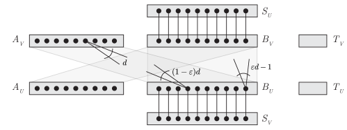
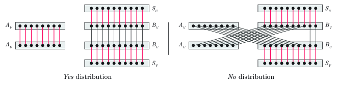
Let us start with the lower bound. Consider the following input distribution, illustrated in the figure below. While we emphasize that this is not the final input distribution that we prove the lower bound with, it provides the right intuition and also highlights some of the challenges that arise in proving the lower bound.
There are four sets of vertices, with and . The vertices are “dummy” vertices, they are adjacent to every other vertex in . While this increases the degree of every vertex in to at least , the vertices cannot contribute much to the output since . The important edges, that determine the output are among the rest of the vertices. In particular, there is always a perfect matching between the vertices and the vertices. Additionally, there is a random Erdös-Renyi graph between and for a suitable expected degree . Now in the distribution, we also add a perfect matching among the vertices (the red matching) but in the distribution, we do not add this matching. Observe that in the case, we can match all of to and all of together, obtaining a matching of size at least . However, in the case, it can be verified that the maximum matching is only at most . Thus, any algorithm that beats 2/3-approximation by a margin more than , should be able to distinguish whether we are in the distribution or in the distribution.
![[Uncaptioned image]](/html/2211.15843/assets/x1.png)
Suppose now that we give away which vertices belong to and for free with no queries, but keep it secret whether a vertex belongs to or . To examine whether a vertex belongs to or , the naive approach is to go over all of its neighbors, and see whether we see an neighbor or not. But because the degree of each vertex is due to the edges to , this requires at least time. But this is not enough. To separate the two cases, one has to actually determine if there are any edges among the vertices or not. Here, the naive approach is to first find a vertex which can be done in time, and then go over all neighbors of in , and examine whether belongs to . Since has neighbors in , this naive approach takes time. We would like to argue that this naive approach is indeed the best possible, and that any algorithm distinguishing the two distributions must make queries to the graph. Unfortunately, this is not the case with the distribution above as we describe next.
Consider the following algorithm. We first start by finding an vertex in time. Then we go over the neighbors of in a random order until we find the first neighbor that belongs to . Note that this takes time. We then do the same for , finding a random neighbor to another vertex in . Since each step of this random walk takes time, we can continue it for steps in total time. Let be the last vertex of the walk. We now examine whether belongs to or in time. We argue that by doing so, there is a constant probability that we can distinguish the case from the case. To see this, observe that in the distribution, every vertex goes to a vertex and every vertex goes to an vertex with probability one. As such, since the walk continues for an even number of steps, the last vertex must belong to with probability 1. But in the distribution, there is a constant probability that we go through an - edge exactly once. In this case, the last vertex of the random walk must belong to . Repeating this process a constant number of times allows us to distinguish the two distributions with probability in merely time!
Correlation Decay to the Rescue:
To get around this challenge, we add edges also among the vertices (while modifying the size of and slightly to ensure that the degrees in and do not reveal any information — see Figure 1). Observe that this completely destroys the algorithm above. In particular, it no longer holds that any vertex goes to an vertex with probability . Rather, there is a probability that we go from to . Hence, intuitively, whether the last vertex of the random walk belongs to or does not immediately reveal any information about whether an - edge was seen or not. We show that indeed, this can be turned into a formal lower bound against all algorithms via correlation decay. First, we show that for suitable , the queried subgraph will only be a tree. We then show that conditioning on the queries conducted far away from a vertex , the probability of being an or vertex will not change, and use this to prove that the algorithm cannot distinguish the and distributions.
2.2 The Algorithms of Theorems 1.2 and 1.3
We now turn to provide an overview of the techniques in obtaining the (almost) 2/3-approximation of Theorem 1.2, and the -approximation of Theorem 1.3 for bipartite graphs.
An (Almost) 2/3-Approximation via EDCS:
The edge-degree constrained subgraph (EDCS) introduced by Bernstein and Stein [10, 11] has been a powerful tool in obtaining an (almost) -approximation of maximum matching in various settings including dynamic algorithms [10, 11], communication complexity [3], stochastic matchings [3], and (random order) streaming [9, 2]. In this work, we use it for the first time in the sublinear time model. In particular, both Theorems 1.2 and 1.3 build on EDCS.
For a parameter (think of it as a large constant), a subgraph of a graph is a -EDCS of if all edges in satisfy and all edges satisfy . The main property of EDCS, proved first by [10, 11] and further strengethened in [3, 4], is that for any , any -EDCS includes a approximate maximum matching of its base graph .
It is not hard to see that finding any -EDCS of the whole input graph requires queries.333In fact, finding the edges of any constant approximate matching requires time. Our focus throughout this paper is on estimating only the size of the maximum matching. Therefore, instead, we first sub-sample some fraction of the edges (or pairs in the adjacency matrix model) of for some fixed in time and construct an EDCS over those edges. Building on an approach of Bernstein [9] in the random-order streaming setting, this can be done in a way such that at most edges in the whole graph remain underfull, i.e., those that do not satisfy property . The union of the set of underfull edges and the EDCS can be shown to include an (almost) 2/3-approximation. The next challenge is that we do not have the set . However, to estimate the maximum matching of , it suffices to design an oracle that upon querying a vertex , determines whether it belongs to an approximately optimal maximum matching of and run this oracle on a few randomly sampled vertices. To do so, we build on a local computation algorithm (LCA) of Levi, Rubinfeld, and Yodpinyanee [19] (which itself builds on a result of Yoshida, Yamamoto, and Ito [24]) that takes time to return if a given vertex belongs to some -approximate matching of its input graph, where here is the maximum degree. Modifying by getting rid of its high-degree vertices, we show the algorithm of [19] can be used to -approximate the size of the maximum matching of in time. Picking sufficiently small, we arrive at an algorithm that obtains a -approximation in time.
Going Beyond -Approximations:
It is known that the (almost) -approximation analysis for EDCS is tight. That is, there are instances on which the EDCS does not include a better than -approximation. However, a characterization of such tight instances of EDCS was recently given in the work of Behnezhad [6] that we use in beating -approximation. Consider a -EDCS , for sufficiently large constant , that does not include a strictly better than 2/3 approximation of -approximation for some small . The characterization divides the vertices into two subsets and depending on their degrees in . Then shows that there must be an (almost) 2/3-approximate matching in the induced bipartite subgraph that is far from being maximal. Namely, it leaves an (almost) 1/3-approximate matching in that can be directly added to . Interestingly, this characterization coincides with our lower bound construction! The set , here, corresponds to the set in the lower bound and the set corresponds to . This essentially reduces the problem to showing that our lower bound construction can indeed be solved in time for all choices of the degree .
Here we show why our lower bound construction fundamentally cannot lead to a better than time lower bound. Indeed the ideas behind our algorithm for Theorem 1.3 are very close. First, suppose that . In this case, we can random sample a vertex in and examine the / value of each of its neighbors in total time to see if it has any neighbors, thereby solving the instance. So let us suppose that . Now in this case, we can first sample a vertex in and list all of its neighbors in time. Since the vast majority (i.e., all but one) of the neighbors of go to , we have essentially found vertices in in time. Repeating this times, we find all of the vertices in total time. We note that the final running time of our algorithm in Theorem 1.3 is only and not since the bottleneck is in finding the EDCS and estimating the maximum matching size of as discussed above. For a more detailed high level overview of the algorithm, see Section 6.
3 Preliminaries
Notation:
Throughout this paper, we let to denote the input graph. We use and to denote the number of vertices and number of edges of the input graph . Also, we use to show the maximum degree, to show the average degree, and to show the size of the maximum matching of graph .
Throughout this paper, for and , we say is an approximation of up to a multiplicative-additive error of (), if . Also, we use to hide factors.
Problem Definition:
Given a graph , we are interested in estimating the size of the maximum matching of . The graph is given in one of the following representations:
-
•
Adjacency Matrix: In this model, the algorithm can query a pair of vertices . The answer is 1 if there is an edge between and , and 0 otherwise.
-
•
Adjacency List: In this model, a list of neighbors of each vertex is stored in arbitrary order in a list. The algorithm can query the ’th element in the list of neighbors of a vertex. The answer is empty if the ’th element does not exist.
Random Greedy Maximal Matching:
Let be the input graph and be a random permutation over all possible permutation of edges . A random greedy maximal matching can be obtained by iterating over with respect to the permutation and constructing a matching by adding edges one by one if they do not violate the matching constraint.
Probabilistic Tools:
In this paper, we use the following standard concentration inequalities.
Proposition 3.1 (Chernoff Bound).
Let be independent Bernoulli random variables, and let . For any ,
Proposition 3.2 (Hoeffding’s Inequality).
Let be independent random variables such that . Let . For any ,
Graph Theory:
We use the following classic theorem by König’s.
Proposition 3.3 (König’s Theorem).
In any bipartite graph, the size of maximum matching is equal to the size of the minimum vertex cover.
4 The Lower Bound
In this section, we prove the lower bound of Theorem 1.1.
To prove Theorem 1.1, we first give an input distribution in Section 4.1. We then prove that any deterministic algorithm which with probability at least .51 (taken over the randomization of the input distribution) returns a -approximation of the size of maximum matching of the input must make at least queries to the graph. By the ‘easy’ direction of Yao’s minimax theorem [23], this also implies that any randomized algorithm with success probability .51 over worst-case inputs must make at least queries to obtain a -approximation.
4.1 The Input Distribution
We start by formalizing the input distribution. Let , where is as in Theorem 1.1, let be a parameter which controls the number of vertices and let . In our construction, we assume , , , and are all integers; note that this holds for infinitely many choices of . For , we construct an -vertex bipartite graph . We first categorize the vertices in , then specify its edges.
The vertex set:
The vertex set is composed of four distinct subsets and similarly is composed of . Throughout, we may write to respectively refer to sets , , , and . In our construction, we will have
We randomly permute all the vertices in and use to denote the -th vertex of in this permutation. We do the same for .
The edge set:
For the edge-set , we give two distributions: in distribution the maximum matching of is sufficiently large, and in distribution the maximum matching of is sufficiently small. The final input distribution draws its input from with probability 1/2 and from with probability 1/2. The following edges are common in both disributions and :
-
•
All vertices in (resp. ) are adjacent to all of (resp. ).
-
•
For any , we add edges and to the graph. In words, there are perfect matchings between and and between and .
-
•
Let be the set of all -regular graphs between and such that for all , . We draw one regular graph from uniformly at random and add its edges to .
-
•
Let be the set of all graphs between and such that for all , for all , and for all , . We draw one regular graph from uniformly at random and add its edges to .
-
•
Let be the set of all graphs between and such that for all , for all , and for all , . We draw one regular graph from uniformly at random and add its edges to .
-
•
For all we add edge to .
The following edges are specific to and respectively:
-
•
In , we additionally add edges and for all .
-
•
In , we additionally add edges and for all .
This concludes the construction of graph . We also emphasize that the adjacency list of each vertex includes its neighbors in a random order chosen uniformly and independently.
Finally, we note that we give away the bipartition of the graph for free. Additionally, we also give away which of the sets any vertex belongs to. What is crucially hidden from the algorithm, however, is whether a vertex belongs to or .
4.2 Basic Properties of the Input Distribution
The following bounds on vertex degrees follows immediately from the construction.
Observation 4.1.
For any graph drawn from or with probability 1 it holds that:
-
1.
for all .
-
2.
for all .
-
3.
for all .
Since for any vertex , we know which of the sets it belongs to, Observation 4.1 implies we know the degree of every vertex in the graph before making any queries. Thus, there is no point for the algorithm to make any degree queries.
Lemma 4.2.
Let and . Then it holds with probability 1 that
This, in particular, implies that any algorithm satisfying the condition of Theorem 1.1 must be able to distinguish whether a graph drawn from distribution belongs to the support of or with probability at least .
Proof.
For , we take edges for , for , and for . Since none of the edges have the same endpoint, the union creates a matching with size which implies .
For , we take as a vertex cover. Note that there is no edge in the induced subgraph between vertices of . The proof follows by König’s Theorem since there exists a vertex cover with vertices.
Furthermore, if be a constant, since (if we choose sufficiently smaller than ), any algorithm satisfying the condition of Theorem 1.1, must be able to distinguish whether a graph drawn from distribution belongs to the support of or with probability at least . ∎
Remark 4.3.
Note that our construction can be slightly modified to have a perfect matching in . We can add a perfect matching between vertices of and to have a matching of size . Therefore, our lower bound also holds for the case that the has a perfect matching.
4.3 Queried Edges Form a Rooted Forest
Here and throughout the rest of the paper, we use to denote the induced subgraph of excluding all the dummy vertices in . Our main result of this section is that any algorithm that makes at most queries to graph , only discovers a rooted forest in :
Lemma 4.4.
Let be any algorithm making at most queries to graph . Let be the empty graph on the vertex set of , and for let be the subgraph of that discovers after queries. The following property holds throughout the execution of with probability : For any , if the ’th query is to the adjacency list of a vertex and returns edge then either or if then is singleton in . Equivalently, this implies that each can be thought of as a rooted forest where may only include one edge and if discovered by querying , then becomes a leaf of in .
Remark 4.5.
Our proof of Lemma 4.4 crucially relies on the fact that the adjacency list of each vertex is randomly permuted in the input distribution. However, we emphasize here that our proof holds even if the internal permutation of the -neighbors of a vertex in the adjacency list of is adversarial. This implies, in particular, that if we condition on the high probability event of Lemma 4.4, the internal permutation of the -neighbors will still be uniform.
To prove Lemma 4.4, we first bound the number of edges of that we see with queries.
Claim 4.6.
Any algorithm that makes queries to , discovers at most edges of with probability .
Proof.
Since we assume makes at most queries, there will be at most vertices for which the algorithm makes more than adjacency list queries. For each of these vertices, we assume that we discover all their neighbors in that is at most , which in total is edges.
Now let be the set of vertices for which makes at most queries. For each new query to a vertex , since there are edges to in and that we have already made at most queries to , the new query goes to with probability at most . Next, let be the indicator of the event that the ’th query to discovers a edge. From our earlier discussion, we get . Moreover, these ’s are negatively correlated. Hence, denoting , we get and can apply the Chernoff bound to obtain that with probability at least ,
concluding the proof. ∎
Next, we show that conditioning on the fact that we can discover at most edges, the probability of having an edge between any pairs of vertices is at most . To give an intuition of why this claim holds, assume that instead of the regular graphs between and (similarly between and , and and ), we have an Erdos-Renyi with the same expected degree as the regular graphs. Since the degree of each regular graph is , then the probability of having an edge between a pair of vertices must be since the existences of edges are independent. However, since we draw a random -regular graph, edge realizations are not independent the same argument does not work. But using careful coupling, we prove that the same claim holds for this construction.
Claim 4.7.
Let us condition on the high probability event of Claim 4.6 that the algorithm has discovered at most edges in . Then for any pair of vertices such that is not among the discovered edges, the probability that is an edge in is at most .
Proof.
Let and . Also, assume that by index of a vertex we mean the index in the permutation of its corresponding subset in the construction. There are three possible cases for the type of subsets that and belong to:
(Case 1) :
note that since the algorithm makes at most queries, using Chernoff bound, it is easy to see that at least a constant fraction of perfect matching edges in the induced subgraph of remains undiscovered. If and both belong to , the probability of having an edge between the pair is at most since we only have a perfect matching between vertices with the same indices in and for , and vertices are randomly permuted.
For the other two cases, we bound the probability of having an edge between and by considering two possible scenarios. First, the probability that both and have the same indices is equal to . Next, assume that and have different indices. Let be the set of all graphs in such that all of them have the edge . Also, let be the set of all graphs in with no edge between pair . In the next two cases, we use coupling to show that conditioned on discovered edges, we have which implies that the probability of having an edge for a pair is at most .
(Case 2) :
without loss of generality, assume that and . First, note that with a probability of , the index of and is the same, which implies that there is an edge between and . Let denote the index of vertex . Now assume that . We claim if there exists edge , then there are at least edges such that , , , and the induced subgraph of these four vertices only has two edges and .
Since the number of incident edges of to is at most , then there are at least vertices in that are not connected to . Also, we exclude the vertex with index in from this set. Let be the set of such vertices in . Hence, . Furthermore, by the construction, each vertex has at least neighbors in with an index not in . Hence, there are at least edges between vertices of and with endpoints having different labels. Moreover, at most of these edges are incident to an edge that one of its endpoints is . Therefore, there are at least edges that satisfy the claimed properties where the inequality follows by the choice of .
Now assume that we remove all edges that we discovered so far. Since we discover at most edges, by removing these edges we still have edges with mentioned properties. Let be such an edge where and . We construct a graph by removing edge and , and adding edges and . If the original graph is in (), the new graph is in () according to the construction since we only change the random regular bipartite graph between and without changing the degrees. We construct a bipartite graph where each vertex of the first part represents a graph in and each vertex in the second part represents a graph in . For each vertex in the first part, we connect it to the vertices of the second part that can be produced by the above operation. Thus, the degree of vertices in the first part is at least . On the other hand, each vertex in the second part is connected to at most vertices of the first part since the degree of each and is at most in the induced subgraph of . Counting the edges from both sides of the constructed bipartite graph yields
(Case 3) or :
without loss of generality, assume that and . With the same argument as the previous case, the probability that both and have the same index is . Moreover, since the degree of the induced subgraph of differs from the previous case by a constant factor, with the same reasoning as the previous part, the probability that there exists an edge between and is at most .
Therefore, conditioning on the discovered edges, the probability of having an edge , is at most ∎
Now we are ready to complete the proof of Lemma 4.4.
Proof of Lemma 4.4.
First, we prove that for any , if two vertices are non-singleton in and , then there is no edge between and in graph . This will imply that any time that we discover a new edge of a non-singleton vertex in , it must go to a vertex that is singleton in . We prove this by induction on . For , the graph is empty and so the claim holds. Suppose that there are no undiscovered edges among the non-singleton vertices of . We prove that this continues to hold for . If , i.e., if we do not discover any new edge of at step , then the claim clearly holds. So suppose that we query some vertex and find an edge at step . It suffices to show that in this case, will not have any non-singleton neighbors in other than . To see this, recall by Claim 4.6 that there are at most non-singleton vertices in . Fixing any such vertex with , we get by Claim 4.7 that the conditional probability of being an edge in is at most . By a union bound over all choices of , we get that the probability of having an edge to any of the non-singleton vertices of is . Finally, since by Claim 4.6 there are at most steps where we discover any edge of , the failure probability over all the steps of the induction is . Hence, the claim is true throughout with probability at least .
We proved above that by querying an already non-singleton vertex , its discovered neighbor must be singleton w.h.p. We will now prove that this also holds if itself is singleton. As discussed, the number of non-singleton vertices in is by Claim 4.6. For each of these vertices , the conditional probability of having an edge to is at most by Claim 4.7. Hence, the expected number of edges of to non-singleton vertices is . Since has edges in and its adjacency list is uniformly sorted, the probability of discovering one of such edges of is at most . A union bound over all queries of the algorithm implies that with probability , any time that we query a singleton vertices of , its discovered edge will not be to another non-singleton vertex of . ∎
4.4 The Tree Model
In our proofs, we condition on the high probability event of Lemma 4.4 that for any forms a rooted forest. Under this event, we prove that the algorithm cannot distinguish the distribution from the distribution.
Recall that from our definition in Lemma 4.4, every vertex in for any is a vertex in set . Given the forest , we do not necessarily know for a given a vertex in whether it belongs to or (but if it belongs to we know this since recall all the vertices are given for free by the distribution). Inspired by this, we can see each vertex in as a random variable taking one of the values . Importantly, depending on the value of we have a different distribution on what values its children in the tree will take. This distribution is also different for the and distributions. For example, in the distribution all children of any vertex will be vertices whereas in the distribution there is a small chance of seeing an child. We prove that although these distributions are different for the and distributions, no algorithm can distinguish (with a sufficiently large probability) whether the observed forest was drawn from or .
The proof consists of multiple steps. First, in Section Section 4.5, we prove a correlation decay property on the tree. Then equipped with the correlation decay property, we are able to show the probability of seeing the same forest by the algorithm in a and is almost the same which implies that the algorithm cannot decide if the graph is drawn from or .
4.5 Correlation Decay
Lemma 4.8 below is our main result in this section. Before stating the lemma, let us start with some definitions. Consider a tree of any arbitrary depth rooted at vertex . We say is --free if no vertex in with distance at most from the root belongs to . We also use to denote the total number of vertices of distance at most from the root in . With a slight abuse of notation, we may also use to denote the event that the sub-tree of rooted at vertex by the end of the algorithm (i.e., when ) is exactly the same as .
Lemma 4.8.
Let be any vertex, , and let be any --free tree. Let and each be an arbitrary outcome of from and the entire forest excluding the sub-tree of . Letting and assuming that , we have
and
Proof.
Call a vertex an internal vertex if it has distance at most from . Note that is the number of internal vertices in . We say a subset of internal vertices form an internal path in a tree if for any , is the parent of in , and additionally each , for , only has one child in .
We use the following two auxiliary Claims 4.9 and 4.10 to prove Lemma 4.8.
Claim 4.9.
Suppose that every vertex in has at least one non-internal descendant. Then must have an internal path of length at least .
Proof.
Suppose for contradiction that does not have any internal path of length . Construct a tree by contracting all maximal internal paths of (of any length). Since every vertex in has a non-internal descendant, which is of distance at least from the root by definition, and every contracted path has a length less than , every vertex in must have a descendant of distance at least from the root. Furthermore, every vertex in must have at least two children. As such, we get that must have vertices, a contradiction. ∎
The proof of Claim 4.10 below is involved; we state it here and present the proof in Section 4.5.1.
Claim 4.10.
Let be an internal path in of length such that each is the parent of . Let be the sub-tree of rooted at vertex and let and be any two events on the vertices outside ’s sub-tree. Then
and
We are now ready to present the proof of Lemma 4.8. Given the tree , to measure the probability of actually happening we start by querying from the same tree topology. That is, if some vertex has children in , we reveal children of from the distribution and measure the probability that the resulting tree is exactly the same as . First, let us measure the probability that the resulting tree is indeed --free. That is, no internal vertex in the queried subtree is an vertex. To do this, take an internal vertex in . Conditioned on either of or , the probability of being an vertex is at most since every vertex in has at most one neighbor, has degree , and its adjacency list is uniformly sorted. On the other hand, since the total number of internal vertices in is , by a union bound, the probability of seeing at least one vertex is at most . Let us condition on the event that we see no internal vertex. This only multiplies the final probability of occuring by some factor.
Conditioned on the observed tree being --free, note that if some internal vertex in the tree has no non-internal descendants, then indeed its sub-tree exactly matches . So let us peel off all such sub-trees, arriving at a tree where every internal vertex has at least one non-internal descedntant. From Claim 4.9, we get that there must be a an internal path of length at least in this tree. Applying Claim 4.10, the probability of happening remains the same up to a factor of , no matter what we condition on above . Thus, we can peel off the whole sub-tree of and repeat. Assuming that we repeat this process times until we peel off all vertices, we get that the probability of occuring under and is the same up to a factor of . Finally, note that since every time we peel off the sub-tree of an internal path, we remove internal vertices in the path, and so is at most the number of internal vertices. This completes the proof of Lemma 4.8. ∎
4.5.1 Correlation Decay on Internal Paths: Proof of Claim 4.10
In this section, we present the proof of Claim 4.10, which as discussed implies correctness of Lemma 4.8.
Proof of Claim 4.10.
For any we define
We claim that for both distributions and , and for any ,
| (1) |
To see this, let us first focus on . We have
| (2) |
Let us now examine . Given that , vertex has exactly neighbors in graph . Among them, either or neighbors of are in . Additionally, since has exactly one child (by definition of internal paths) then the conditional event may only reveal the /-value of one neighbor of , which would be its parent. Since the adjacency list of vertex is randomly sorted, its discovered child belongs to with probability at least and at most . Thus,
On the other hand, since every vertex in has at least and at most neighbors in ,
Replacing these two bounds in 2, we indeed arrive at the recursion of 1 for .
The calculation for is similar. In particular, as in 2, we have
We have since almost fraction of neighbors of each vertex go to , and we have since each vertex has at most one neighbor among its neighbors. Replacing these into the inequality above, implies the recursion of 1 for .
The following claim gives an explicit (i.e., non-recursive) bound for and as a function of just and .
Claim 4.11.
Let
and
Then for any , we have
Proof.
First, we note a couple of useful properties of and that all can be verified from their definitions:
| (3) |
To prove the stated bounds on and we use induction on . For the base case , directly applying 1 we get
Similarly, we have
We now turn to prove the induction step for , assuming that it holds for . Let us start with . We have
| (From 1.) | ||||
| (By the induction hypothesis.) | ||||
| (By 3.) |
Moreover, for we have
| (From 1.) | ||||
| (By the induction hypothesis.) | ||||
| (Since for .) | ||||
| (By 3.) |
This completes the proof of Claim 4.11. ∎
Observe that since and so either or . Combined with Claim 4.11, we get that
| (Since .) | ||||
Observe that the conditioning determines the values of and . However, for large enough , as we see above, the dependence of on and vanishes. In other words, by changing the conditioning the value of for only changes by a factor. The same also holds for . As such, whether vertex belongs to or is essentially independent of the events above the root vertex . To see why this implies Claim 4.10, take for example the distribution and note that
Since and remain the same up to a factor by changing the conditioning to , we arrive at the desired inequality of Claim 4.10 for the distribution. The proof for is exactly the same. ∎
4.6 Limitation of the Algorithm
Let us define to be the set of all discovered edges of by the algorithm. Also, let , where here is directed and is the parent of in the forest of discovered edges.
Claim 4.12.
With high probability, any algorithm that makes at most queries, discovers at most of edges in subgraph with one endpoint in .
Proof.
The proof is similar to the proof of Claim 4.6. Since we assume makes at most queries, there will be at most vertices for which the algorithm makes more than adjacency list queries. For these vertices, we assume that finds its edge in with one endpoint in (note that the degree of vertices in is one and each vertex of is connected to at most one vertex of ).
Now let be the set of vertices for which makes at most queries. For each new query to a vertex , since there are edges to in and that we have already made at most queries to , the new query goes to a vertex in with probability at most . Hence, by applying the Chernoff bound, with probability at least , there are at most edges in subgraph with one endpoint in . ∎
Lemma 4.13.
Suppose that the algorithm has made queries for some . Then with probability of , all the following hold:
-
(i)
has found at most vertices in total for all subtrees for up to a distance from root .
-
(ii)
has not found any edge in with one endpoint in in subtree up to distance from root , for all .
-
(iii)
Conditioning on what has queried so far, the probability of each edge in belonging to is .
Proof.
We prove the lemma using induction. For , trivially the statement is true. Now assume that the lemma holds for and makes a new query. If the new queried edge is an edge to , we are done since none of the conditions in the lemma statement will change. So we assume that the newly queried edge is in . We prove each of the three claims separately.
Induction step for (ii):
if the newly queried edge is between and , the probability that one of its most recent predecessors is an edge in is using the induction hypothesis (iii). Since can discover at most edges in with one endpoint in by Claim 4.12, then with probability at least , the statement of (ii) remains true throughout all the steps of the induction.
Induction step for (i):
the probability that at least one of the most recent predecessors of the newly queried edge is an edge in is using the induction hypothesis (iii). Since discovers at most edges of by Claim 4.6, then with probability at least , the statement of (i) remains true throughout all the steps of the induction.
Induction step for (iii):
let be a discovered edge in the forest ( is parent of ). First, we condition on , otherwise, the probability of being an edge in is zero. Note that has at least neighbors in that are not the parent of in the forest . By Claim 4.12, discovers at most edges in subgraph with one endpoint in . Hence, at most of neighbors of in have an edge with one endpoint in in their subtree. Furthermore, by Claim 4.6, at least neighbors of in , have at most vertices in their subtree. Also, note that by proof of Lemma 4.4, neighbors of in that are not adjacent to in the forest are singleton vertices in the forest. Let be the union of (1): children of in the forest such that each of them has no edge with one endpoint in their subtree up to distance , and each of them has vertices in their subtree up to distance , (2): the neighbors of in that are singleton in the forest. Hence, we have .
By (i) and (ii), if then there are at most vertices in subtree up to distance from root , and there is no edge in subtree with one endpoint in up to distance from the root. Thus, if , then is not an edge in . Now assume that . Note that in , there is no neighbor of with label and in , there is exactly one neighbor in . Therefore, for , the probability of is zero. Now assume that the graph is drawn from . Hence, exactly one of is in (if parent of is then the probability of being in is zero). We prove that each of can be in with almost the same probability using a coupling argument.
Let be the subset that vertex belongs to (. We say is a profile for labels of vertices . Therefore, exactly one of is equal to and all others are equal to which implies that there are different possible profiles. Assume that and are two different profiles. Let be a vertex with label in and be a vertex with label in . By Lemma 4.8, the probability of sampling subtree below with label is the same up to a factor of . Similarly, the probability of sampling subtree below with label is the same up to a factor of . Since , then the probability of having profile and is the same up to a factor. Therefore, the probability of having one specific to be in is since . ∎
4.7 Indistinguishability of the and distributions
We define a bad event to be the event of discovering more than vertices in total for all subtrees for up to a distance from root , or has found at least one edge in with one endpoint in in subtree up to distance from root for at least one . By Lemma 4.13, the bad event happens with probability . For the next lemma, we condition on not having a bad event.
Lemma 4.14.
Let us condition on not having the bad event defined above. Let be the final forest found by algorithm on a graph drawn from after at most queries. Then, the probability of querying the same forest in a graph that is drawn from is at least almost as large, up to multiplicative factor.
Proof.
First, we define hybrid distributions as follows. Distribution can be obtained by sampling from until the -th level in any tree in the forest, and then sampling from below the -th level. Hence, is exactly the same as and is the same as . Our goal is, starting from a forest sampled according , to inductively show that we can switch from to with only negligble total decrease in the probability.
To formalize our coupling argument, recall the notion of special edges from the input distribution: In , edges in are special; in , every vertex in has one special edge to all forming a matching. We also extend the definition of bad events to and hybrid distribuitons to include bad events in subtrees originating from special edges.
Consider the forest found by algorithm on a graph drawn from , and let denote the forest as well as any choice of its special edges in all levels (arbitrarily, conditioning on not having a bad event). We compare the probability of seeing when making the same queries when the oracle samples its answers from vs . We can couple the sampling for the two distributions so that it is identical for everything in levels (including the choice of special edges), and also for levels in all the sub-trees that are not descendants of special level- edges.
For each special edge in the -th level, the label of vertex is when sampling from and when sampling from . Below this vertex (aka levels ), both distributions and sample according to . Thus, by Lemma 4.8, the probability of sampling the subtree below is the same regardless of the label of , up to a factor of .
Let denote the set of vertices pointed to by -th level special edges. By the argument in the previous paragraphs, we have
| (4) |
Let denote the event of having no bad events corresponding to level- special edges. Summing over (4) for all valid choices of special edges, we have the following:
We can now bound the total distribution shift across all hybrid steps:
| (By Lemma 4.13.) | ||||
This completes the proof of Lemma 4.14. ∎
Proof of Theorem 1.1.
Note that the probability of having the bad event that we defined is . Conditioning on not having the bad event, by Lemma 4.14, the distribution of the outcome that the algorithm discovers is in total variation distance for and . Therefore, the algorithm is not able to distinguish between the support of two distributions with constant probability. According to our construction, the size of the maximum matching of both and is , and in both cases, the input graph is bipartite. ∎
5 An (Almost) 2/3-Approximation
Throughout this section, we introduce an algorithm that achieves an almost 2/3 approximation in sublinear time in both the adjacency list and matrix models, thereby proving Theorem 1.2. Specifically, we prove the following theorems, which further formalize Theorem 1.2 of the introduction.
Theorem 5.1.
For any constant , there exists an algorithm that estimates the size of the maximum matching in time up to a multiplicative-additive factor of with high probability in both adjacency matrix and adjacency list model.
Theorem 5.2.
For any constant , there exists an algorithm that estimates the size of the maximum matching in time up to a multiplicative factor of with high probability in the adjacency list model.
One key component of our algorithm is the edge-degree constrained subgraph (EDCS) of Bernstein and Stein [10]. An EDCS is a maximum matching sparsifier that has been used extensively in the literature on maximum matching in different settings such as dynamic and streaming. It is known that an EDCS contains an almost 2/3-approximation of the maximum matching of the original graph. Formally, we can define EDCS as follows:
Definition 5.3 (EDCS).
For any and , subgraph is a -EDCS of if
-
•
(Property P1:) for all edges , , and
-
•
(Property P2:) for all edges , .
We use a more relaxed version of EDCS in our algorithm that first appeared in the literature on random-order streaming matching [9]. Let be a subgraph of such that it satisfies the first property of the EDCS (P1) in Definition 5.3 for some , and be the set of all edges of that violate the second property of EDCS (P2). It is possible to show that the union of and contains an almost 2/3-approximation of the maximum matching of the original graph.
| Variable | Definition | Intuition | ||||
|---|---|---|---|---|---|---|
| See Algorithm 1 | Relaxed EDCS | |||||
| Edges not sampled by Algorithm 1 | ||||||
| See Algorithm 1 |
|
|||||
|
||||||
|
||||||
| Edges in can augment | ||||||
| defined in Algorithm 3 | is non-trivially sparse | |||||
|
|
Definition 5.4 (Bounded edge-degree).
A graph has a bounded edge-degree if for each edge , we have .
Proposition 5.5 (Lemma 3.1 of [9], (Relaxed EDCS)).
Let and be parameters such that , . Let be a subgraph of with bounded edge-degree . Furthermore, let be a subgraph that contains all edges in such that . Then we have .
An Informal Overview of the Algorithm:
In the next few paragraphs, we give an informal overview so the readers know what to expect. Algorithm 1 consists of two main parts. Let initially be an empty subgraph. First, in rounds ( is the parameter of EDCS), we sample pairs of vertices in the graph (in the adjacency list model, we sample edges). After sampling in each round, we update the bounded edge-degree subgraph . For each edge , if the , we add it to . This change can affect the bounded edge-degree property of . In order to avoid this issue, we iterate over incident edges of to remove edges with degree more than . Note that at most one neighbor of each and will be deleted after this iteration. Since , this part can be done in time. Furthermore, since we have chosen enough random edges, the number of unsampled edges in the graph that violate Property (P2) of the EDCS is relatively small. Note that when we remove edges to fix Property (P1), it is possible that an edge that was previously sampled but rejected due to the high -degree, now has a lower -degree and thus violates Property (P2). However, in the analysis, it will be sufficient to consider only unsampled edges that violate Property P2. More specifically, we show that the total number of unsampled violating edges is .
Note that the union of approximate EDCS and unsampled violating edges preserves an almost 2/3-approximate maximum matching of the original graph since most of the edges of the graph are unsampled and the unsampled subgraph itself, contains a large matching. Hence, we can apply Proposition 5.5 to the union of and all unsampled violating edges. Also, graph has a low average degree. Hence, it remains to estimate a -approximate matching of graph that has a low average degree. For this part, we use the time local computation algorithms (LCA) of Levi, Rubinfeld, and Yodpinyanee [19] which itself builds on the sublinear time algorithm of Yoshida, Yamamoto, and Ito [24]. In local computation algorithms, the goal is to compute a queried part of the output in sublinear time. One challenge here is that we do not have access to the adjacency list of graph to use the algorithm of [19] as a black box. We slightly modify this algorithm to run in with access to the adjacency matrix or the adjacency list of the original graph . Furthermore, since this algorithm works with the maximum degree, we eliminate some high-degree vertices by losing an additive error. In what follows, we formalize the intuition given in previous paragraphs.
Proposition 5.6 ([19]).
There exists a randomized -approximation local computation algorithm for maximum matching with running time using access to adjacency list.
Lemma 5.7.
Let be a subgraph of graph . Also, let be a local computation algorithm for maximum matching in with running time using access to the adjacency list of . There exists an algorithm with exactly the same approximation ratio that runs in time with access to the adjacency matrix or the adjacency list of .
Proof.
Since algorithm runs in time, it visits at most vertices in the graph. For each of these vertices, we can simply query all their edges in using time having access to the adjacency matrix or the adjacency list of . Therefore, for each vertex that visits, we can construct the adjacency list of the vertex by spending time. ∎
Corollary 5.8.
Let be a subgraph with maximum degree of graph . There exists a local computation algorithm for that for a given vertex , determines if it is in the output of a -approximate maximum matching of with a running time with access to the adjacency matrix or the adjacency list of .
Proof.
The proof follows by combining Proposition 5.6 and Lemma 5.7. ∎
We use the same argument as [9] to show that the average degree of violating unsampled edges is low. The only difference here is that in each epoch, we have sampled edges but the algorithm of [9] use sampled edges which causes us to get weaker bound on the average degree. First, we rewrite a useful lemma from [9] that also holds in our case which shows that in one of epochs of Algorithm 1 the subgraph does not change and the algorithm breaks the loop in Line 3.
Lemma 5.9 (Lemma 4.2 of [9]).
Let and be a subgraph with no edges at the beginning. An adversary inserts and deletes edges from with the following rules:
-
•
delete an edge if ,
-
•
insert an edge if .
Then after at most insertions and deletions, no legal move remains.
Note that in the original version of this lemma in [9], the constraint for insertion rule is , but essentially the same proof carries over without any change. Therefore, the same bound still holds for this weaker version. By Lemma 5.9, in at least one of rounds of Algorithm 1, the subgraph remains unchanged and the algorithm exits the loop in Line 3. Next, we prove that after the algorithm exits in Line 3 because of no change in , the number of remaining unsampled edges that violate the second property of EDCS (P2) is small. (The proof of this lemma is similar to Lemma 4.1 of [9].)
Next, after the algorithm exits the loop in line 3 because of no change in , the number of remaining unsampled edges that vaiolate the second property of EDCS (P2) is small. Assume that the algorithm sample fraction of edges of the original graph at random and constructs the bounded edge-degree subgraph . Behnezhad and Khanna [7] (see Claim 4.16 of the paper) proved that the number of unsampled violating edges is at most . In our case, by the choice of and . We restate the lemma with this specific .
Lemma 5.10.
Let be the subgraph consisting of violating unsampled edges in Line 7 of Algorithm 1. Then we have with probability at least .
Claim 5.11.
Let be the set of sampled edges in Line 4 of Algorithm 1. Then running the Algorithm 2 for one epoch to update can be done in time. Moreover, the whole process of constructing takes time in both adjacency lists and matrix models.
Proof.
Since Algorithm 1 samples at most pairs of vertices, we have . Algorithm 2 iterates over the edges one by one in each epoch and adds edge to if . Adding this edge can cause incident edges of and to have a degree higher than in . In order to remove those edges, we iterate over edges of and in and remove the first edge with a degree higher than . This can be done in since each vertex has at most neighbors. Thus, the running time of each epoch is . Since we have epochs, the total running time is by our choice of . ∎
Lemma 5.12.
Let be as defined in Algorithm 1. Then there exists a -approximation LCA algorithm for maximum matching of with preprocessing time and additional time per query.
Proof.
Combining Lemma 5.10 and our choice of , the average degree of graph is . Note that the algorithm of [19] works with maximum degree. In order to use this algorithm as a subroutine in Line 9 of our algorithm, we ignore vertices of high degree and find a -approximate maximum matching in the remaining graph by losing an additive error which depends on . However, we do not have access to the degree of vertices in since we do not have access to the adjacency list of .
For each vertex , we sample vertices to estimate the degree of . Let be the number of neighbors that are in and be our estimate for the degree of in . Using Chernoff bound, we get
A union bound over all vertices yields that with a probability of , we have an additive error of at most for the degree of all vertices.
Now we ignore the vertices with estimated degrees larger than . Combining the additive error bound for degree estimation and the fact that the average degree of the graph is at most , the total number of ignored vertices is at most .
For the remaining vertices, the maximum degree is at most . Moreover, for an edge in we can check if the degree of the edge is smaller than or not (the edge belongs to or not). Thus, we can run the algorithm of Corollary 5.8 in since the maximum degree is and either we have access to adjacency matrix or adjacency list of . Also, note that since the additive error is , the approximation ratio cannot be worse than . Proof of claim follows from using as the parameter. ∎
Claim 5.13.
.
Proof.
The fact that is a subgraph of implies the second inequality. Let be the subgraph consisting of unsampled edges. By Lemma 2.2 of [9], we have with high probability. To see this, we sample fraction of edges, however, in [9], they sample edges. Hence, the graph has more unsampled edges and therefore a larger matching compared to unsampled edges of [9]. Moreover, by Proposition 5.5, we have . Therefore, we obtain
Proof of claim follows from using as the parameter. ∎
Lemma 5.14.
let be the output of Algorithm 1 on graph . With high probability,
Proof.
Let be the -approximate matching of Lemma 5.12 on graph and be the indicator if vertex is matched in or not. By Claim 5.13, we have
| (5) |
Because the number of matching edges is half of the matched vertices,
Thus,
| (6) |
Using Chernoff bound and the fact that is the sum of independent Bernoulli random variables, we have
Hence, with probability ,
Plugging 5 in the above range implies
Since and , we get
Proof of lemma follows from using as the parameter. ∎
Now we are ready to complete the analysis of the 2/3-approximate maximum matching algorithm.
See 5.1
Proof.
We run Algorithm 1. By Lemma 5.14, we obtain the claimed approximation ratio. The proof of running time follows from combining Claim 5.11, Lemma 5.12, and . ∎
Multiplicative Approximation for Adjacency List:
In the adjacency list model, we can assume that we are given the degree of each vertex. This assumption is without a loss of generality since we can use binary search for each vertex to find its exact degree. Thus, we know the total number of edges in the graph and if this number is not larger than , then we can use linear time approximation for maximum matching. Equipped with this observation, we assume that , otherwise, the number of edges cannot be more than . Moreover, the size is at least , which implies that we can assume . With this assumption and using standard Chernoff bound, it is not hard to see that we can estimate the size of the maximum matching of with a multiplicative factor by sampling vertices. By the running time of Claim 5.11, preprocessing time of Lemma 5.12, and query time of Lemma 5.12 combined with queries, results in multiplicative -approximation algorithm with running time.
See 5.2
6 Beating 2/3-Approximation in Bipartite Graphs
In this section, we design a new algorithm that gets slightly better than approximation in sublinear time in both the adjacency list and matrix models for bipartite graphs. Our starting point is to use the tight case characterization of the instance that our algorithm in the previous part cannot obtain better than a approximation. Then we use that characterization to design a new algorithm to go beyond . We prove the following theorem, which further formalizes the statement of Theorem 1.3 in the introduction.
Theorem 6.1.
For an absolute constant , there exists an algorithm that estimates the size of the maximum matching in time up to a multiplicative-additive factor of with high probability in both adjacency list and matrix models.
Theorem 6.2.
For an absolute constant , there exists an algorithm that estimates the size of the maximum matching in time up to a multiplicative factor of with high probability in the adjacency list model.
To break -approximation, we build on a characterization of tight instances of EDCS due to a recent work of Behnezhad [6]. In our context, the characterization asserts that if the output of our Algorithm 1 is not already a -approximate matching of for some constant (we did not try to optimize the constant), then there exists a -approximate matching in (defined in Algorithm 1) such that it is far from being maximal in the original graph .
Notation
Let be the input bipartite graph, and let and be as defined in Algorithm 1. Let and be the set of vertices such that and , respectively. Let . Also, fix to be a -approximate matching of . We let and for the rest of this section.
Lemma 6.3 ([6]).
Let and be some constant. If , then both of the following guarantees hold:
-
•
(G1 - contains a large matching )
-
•
(G2 - can be augmented in ) For any matching in , we have
An Informal Overview of the Algorithm:
Let be a -approximate matching of . According to this characterization, if Algorithm 1 does not obtain better than a approximation, then matching preserves the size of matching of and also, it can be augmented using a matching with edges of . By Lemma 6.3, if the matching that we estimate in Algorithm 1 does not obtain better than approximation, then there exists a large matching in that can be augmented using a matching between vertices of .
Therefore, if we want to obtain a better than approximation, all we need is to estimate the size of a constant fraction of a matching in . The first challenge is that we do not know which vertices of are in and which are in . With a similar proof as proof of Lemma 5.12, we can show that it is possible to query if a vertex is matched in in time, since is a subgraph of and its average degree is smaller than . Moreover, for an edge in , we can check if the -degree of the edge is smaller than (the edge belongs to or not), and one endpoint is in and the other one in (the edge belongs to or not) in . Thus, we can run the algorithm of Corollary 5.8. We restate the lemma for subgraph .
Lemma 6.4.
There exists a -approximation LCA algorithm for maximum matching of with preprocessing time and additional time per query.
Since is a subgraph of , by Lemma 5.12, we can query if a vertex is matched in in . So the time to classify if a vertex is in or is since we can query if it is matched in matching or not.
Unfortunately, the subgraph can be a dense graph (possibly with an average degree of ), so it is not possible to run an adaptive sublinear algorithm that adaptively queries if a vertex is in or not while looking for a matching. So we first try to sparsify the graph by sampling edges and constructing several maximal matchings. More specifically, we query pairs of vertices (for and ) and partition the queries to equal buckets. Then we build a greedy maximal matching among those sampled edges of bucket . By this construction and the sparsification property of greedy maximal matching, we are able to show that the maximum degree of subgraph is with high probability for each .
We split the rest of the analysis into three possible cases.
(Case 1) A constant fraction of vertices of are matched in at least one of :
in this case we immediately beat since we found a constant fraction of a maximum matching edges of .
(Case 2) A constant fraction of maximum matching of has both endpoints unmatched in at least one of :
Let be an index of matching that a constant fraction of maximum matching of has both endpoints unmatched. In this case, we prove that it is possible to estimate a constant approximation of the size of the matching between unmatched vertices of in sublinear time.
Let be the same as subgraph , except that we connect each vertex in to dummy singleton vertices. The reason to connect singleton vertices to is that if we run a random greedy maximal matching on , most of the vertices in will match to singleton vertices with some additive error. Thus, if there exists a large matching between unmatched vertices, random greedy maximal matching will find at least half its edges. We sample vertices and test if they are matched in the random greedy maximal matching of . To do this, we use the algorithm of [5] which has a running time of for a random vertex. However, for each vertex that this algorithm recursively makes a query, we have to classify if it is in or since we do not explicitly construct . As we discussed at the beginning of this overview, this task can be done in time. For each maximal matching, the running time for this case is . Therefore, the total running time is for all maximal matchings which is sublinear if we choose sufficiently larger than .
Note that if we are not in one of the above cases, almost all edges of maximal matchings have at most one endpoint in (as a result of not being in Case 1), and almost all edges of the maximum matching of have at least one endpoint matched by all maximal matchings (as a result of not being in Case 2). Thus, if we consider a vertex in , almost all of its incident maximal matching edges go to set . For this case, we now describe how it is possible to estimate the matching of .
(Case 3) Almost every edge of maximum matching of has at least one of its endpoints matched by almost all :
In this case we will show that we can efficiently remove many -vertices, and then repeat the algorithm and and analysis of Cases 1 and 2 (using fresh samples of . Because we can’t keep removing -vertices indefinitely, eventually we have to end up at either Case 1 or 2.
Our goal is henceforth to efficiently identify many -vertices. Suppose that we sample a vertex and check if it is in or . If the sampled vertex is in and is one of the endpoints of maximum matching of , most of its incident edges in are connected to vertices of . Therefore, we are able to find vertices of the set by spending to find a vertex in . Hence, if we sample such vertices, we are expecting to see a constant fraction of vertices of ; we can remove these vertices and run the same algorithm on the remaining graph again. One challenge that arises here is that some of the neighbors of the sampled vertex might be in . To resolve this issue, we choose a threshold and only remove vertices that have at least maximal matching edges that are connected to sampled vertices. This will help us to avoid removing many vertices in each round. Since initially the size of and is roughly the same (up to a constant factor), after a few rounds, we can estimate the size of the maximum matching of . The total running time of this case is also which is the same as the previous case.
In what follows, we present the formal algorithm (Algorithm 3) and formalize the technical overview given in previous paragraphs.
6.1 Analysis of Running Time
We analyze each part of Algorithm 3 separately in this section and at the end, we put everything together. Before starting the analysis of the running time of Algorithm 3, we first restate the following result on the time complexity of estimating the size of the maximal matching by Behnezhad [5].
Lemma 6.5 (Lemma 4.1 of [5]).
There exists an algorithm that draws a random permutation over the edges of the graph and for an arbitrary vertex in graph , it determines if is matched in the random greedy maximal matching of in time with high probability, using adjacency list of , where is the average degree of .
Claim 6.6.
Let be as defined in Algorithm 3. The running time for constructing for all , takes time for all iterations of the algorithm.
Proof.
Fix an iteration in the algorithm. Since we sample pairs of vertices and we have buckets of equal size, each bucket can have at most edges. For each of the buckets, in order to construct the maximal matching we need to iterate over the edges of the bucket one by one which takes time for all buckets. The proof follows from . ∎
Claim 6.7.
The total preprocessing time before all iterations of Algorithm 3 is .
Proof.
Algorithm 3 uses subroutine of Lemma 6.4 to query if a vertex is matched in -approximate matching of during its execution. Thus, by Lemma 6.4, the total preprocessing time needed for the algorithm is . ∎
Claim 6.8.
Every time that Algorithm 3 calculates , it takes time. Furthermore, the total running time for computing in the whole process of algorithm is time.
Proof.
By Lemma 6.4, each query to see if a vertex is matched in -approximate matching of , takes time. Since we sample vertices, we get the claimed time complexity. ∎
Lemma 6.9.
Subgraph has a maximum degree of with high probability.
Proof.
Consider a vertex that is not matched in and has a degree larger than in . The only way that remains unmatched is that none of its incident edges in get sampled in pairs of vertices we sampled. The probability that we sample one of these edges is at least , since there are at most possible pairs of vertices. Thus, the probability that none of these edges sampled in samples when constructing is at most
Taking a union bound over all vertices of the graph completes the proof. ∎
Claim 6.10.
Every time that Algorithm 3 calculates , it takes time. Furthermore, the total running time for computing in the whole process of algorithm is time.
Proof.
By Lemma 6.9, the maximum degree of subgraph is with high probability. Thus, by Lemma 6.5, indicating if a vertex is matched in the random greedy maximal matching of takes time. Moreover, for each vertex in the process of running a random greedy maximal matching local query algorithm, we need to distinguish if it is a vertex in or since we build subgraph on the fly (we cannot afford to build the whole graph at the beginning which takes time). By Lemma 6.4, each of these queries takes time. Therefore, it takes time to calculate each time. Combining with the fact that , we have maximal matchings, the size of set is a constant fraction of , and implies the claimed running time. ∎
Claim 6.11.
Updating vertex set at the end of case 3 in Algorithm 3 takes time. Furthermore, the total running time for computing in the whole process of algorithm is time.
Proof.
Each time that we sample a vertex, we need to test if it is a vertex in . This takes by Lemma 6.4. Since we need to sample vertices of and the size of set is a constant fraction of by Lemma 6.3, we need to sample at most vertices of . Hence, it takes time to find vertices . Each of the vertices has at most neighbors in all maximal matchings which implies that we need to spend time to find and remove vertices of set which completes the proof since . ∎
Now we are ready to complete the analysis of the running time of Algorithm 3.
Lemma 6.12.
The total running time of Algorithm 3 is .
Proof.
The proof follows from combining Lemma 6.4, Claim 6.6, Claim 6.7, Claim 6.8, Claim 6.10, and Claim 6.11. ∎
6.2 Analysis of Approximation Ratio
In this section, we assume that and we prove with this assumption, the algorithm outputs a better than approximation in one of iterations. The proof for the other case where is trivial since the algorithm outputs an estimation which is at least .
6.2.1 Approximation analysis of Case 1: Many -vertices matched in some
Lemma 6.13.
If , then is an estimate for up to a multiplcative-additive factor of with high probability.
Proof.
First, we prove that . Let be as defined in Algorithm 3. Note that since it counts the number of edges in that have both of their endpoints in . Since is the sum of independent Bernoulli random variables, using Chernoff bound we have
Thus, with a probability of at least ,
Moreover, we have that . Since only contains vertices that are not matched in the matching that we found in , we get . On the other hand, by Lemma 6.3, we have . Thus,
where the last inequality holds by our choice of , , and if we choose sufficiently small enough, which leads to our claimed approximation ratio. ∎
6.2.2 Approximation analysis of Case 2: Large matching in (for some )
Lemma 6.14.
If , then is an estimate for up to a multiplcative-additive factor of with high probability.
Proof.
Note that since we connect each vertex of to singleton vertices, most of the vertices of will be matched to singleton vertices when running random greedy maximal matching. Let . The first incident edge of in the permutation of edges is not an edge to singleton vertices with a probability of at most since the maximum degree of subgraph is at most by Lemma 6.9. We denote the vertices of that are not matched with singleton vertices by . Hence, we have the following bounds,
Therefore, using a Chernoff bound, we can show that with a high probability.
Now, we prove that . Let be as defined in Algorithm 3, then we have , since it counts the number of edges in output of random greedy maximal matching with both endpoints in and there are at most vertices of can match to vertices of . Also, each edge is counted at most twice since it has two endpoints in . Thus,
since is the sum of independent Bernoulli random variables. Therefore, with a probability of at least ,
which implies that with the same argument as proof of Lemma 6.13. Now we are ready to finish the proof since
∎
6.2.3 Approximation analysis of Case 3: Almost every edge of maximum matching of has at least one of its endpoints matched by almost all
Lemma 6.15.
Before the start of the -th iteration of Algorithm 3 for : if the algorithm has not terminated yet, then it holds that .
Proof.
In the beginning of the section we assumed that . Note that contains vertices that are not matched by the matching of estimation . Therefore, before the first iteration of the algorithm, by Lemma 6.3, set must contain a matching of size larger than where the inequality follows from our choice of .
We use induction to prove the lemma. Suppose that the algorithm has not terminated before the -th iteration for . Note that since the algorithm has not terminated in the previous iteration for any of the maximal matching , the total number of maximal matching edges between vertices of is at most , which implies that the average degree of a vertex in is at most
Let be the number of edges of that are in one of the maximal matchings. Since we sample vertices of , we have
Since each vertex of have at most neighbors in (because we have maximal matchings), then by using Hoeffding’s inequality, we obtain
Therefore, with high probability, there are at most edges of maximal matchings of sampled vertices with both endpoints in (*).
Now we show that at most vertices of are removed in Line 3 (of Algorithm 3) in the previous iteration. For the sake of contradiction, assume that more than are removed in the previous iteration. Then, we have at least
edges of maximal matching between vertices of since each removed vertex must have at least neighbors in the sampled vertices, which is a contradiction to (*). By induction, before iteration , we have . Also, at most vertices of can be removed in the previous step which implies the claimed bound for iteration . ∎
Corollary 6.16.
Before the start of the -th iteration of Algorithm 3 for : if the algorithm has not terminated yet, then it holds that
Proof.
By Lemma 6.15, we have that
where the last inequality follows from our choice of and . We finish the proof by the fact that the number of vertices of a graph is larger than its matching size. ∎
Observation 6.17.
Suppose that Algorithm 3 does not terminate in iteration . Then, it holds before iteration .
Proof.
Consider maximal matching . Since the algorithm has not terminated in iteration , at least edges of are blocked by maximal matching edges since the algorithm does not find more than edges of matching in case 1 and 2. This means that at least one endpoint of these edges is matched with a vertex in . Thus, we have
where the second inequality follows from Lemma 6.15 and , and the last inequality follows by the choice of , , and . ∎
Lemma 6.18.
Suppose that the Algorithm 3 does not terminate in iteration . Then, at the end of this iteration, the algorithm removes at least vertices of .
Proof.
Since the algorithm does not terminate in iteration for any of maximal matchings, at least edges of are blocked by each of maximal matchings. This means that at least one endpoint of these edges is matched with a vertex in . Thus, there are at least
edges with one endpoint in and one endpoint in in all maximal matchings. Hence, the expected average degree of a vertex in in the subgraph is at least
where the inequality is because . Let be the number of edges of with one endpoint in that is among sampled vertices and one endpoint in . Since we sample vertices of , we have
With the same argument as proof of Lemma 6.15, each vertex of can have at most neighbors in , then by using Hoeffding’s inequality, we get
which implies that with high probability, there are at least edges of maximal matchings with one endpoint in sampled vertices and one in .
Next, we prove for each vertex in , the number of sampled vertices in is small with high probability. Note that each vertex in is sampled with a probability of . Moreover, each vertex in can have at most neighbors in . Let be the expected number of sampled vertices that are connected to in for . Therefore,
where the last inequality holds because of Corollary 6.16. Then, by Chernoff bound
Using a union bound on all vertices of implies that with high probability, each of the vertices of has at most neighbors in among sampled vertices.
For the sake of contradiction, suppose that the algorithm removes less than vertices of at the end of the iteration. This implies that the maximum number of edges between vertices of and sampled vertices is
where the first term is the total number of edges of removed vertices of and the second term is the total number of edges of vertices of that are not removed. Since we proved that with high probability, there are at least edges, then the above upper bound on the number of edges is a contradiction that completes the proof. ∎
6.3 Putting it all together: Beating two-thirds
Lemma 6.19.
If , then the Algorithm 3 terminates in one of iterations.
Proof.
Suppose that the algorithm does not terminate in any of rounds. By Lemma 6.18, in each iteration, the algorithm will remove vertices of . Thus, after iterations, none of the vertices of will remain in the graph. However, plugging in Lemma 6.15, we have . Therefore, either or in iteration , since there is no vertices of to block the matching of . ∎
Lemma 6.20.
The output of Algorithm 3 is a estimate for maximum matching of .
Proof.
If is not a estimate for maximum matching of , then by Lemma 6.19, the algorithm terminates in one of the rounds. Therefore, by Lemma 6.13 and Lemma 6.14, the output is a estimate for maximum matching of . ∎
See 6.1
Proof.
By Lemma 6.20, we obtain the claimed approximation ratio. Also, since we choose to be smaller than in Algorithm 3, the running time is by Lemma 6.12. ∎
Multiplicative Approximation for Adjacency List:
With the same argument as the multiplicative approximation for the adjacency list in the previous section, we can assume . Hence, if , we have by Lemma 6.3. Therefore, with the exact same argument as previous section, using a standard Chernoff bound, for getting multiplicative approximation, we can use and samples for estimation of and . Note that the running time of Claim 6.8 and Claim 6.10 will increase to and , respectively because of the larger number of samples. However, if we choose larger than , the running time of the algorithm will remain by Lemma 6.12.
See 6.2
References
- Abboud and Williams [2014] Amir Abboud and Virginia Vassilevska Williams. Popular conjectures imply strong lower bounds for dynamic problems. In 55th IEEE Annual Symposium on Foundations of Computer Science, FOCS 2014, Philadelphia, PA, USA, October 18-21, 2014, pages 434–443, 2014.
- Assadi and Behnezhad [2021] Sepehr Assadi and Soheil Behnezhad. Beating two-thirds for random-order streaming matching. In Nikhil Bansal, Emanuela Merelli, and James Worrell, editors, 48th International Colloquium on Automata, Languages, and Programming, ICALP 2021, July 12-16, 2021, Glasgow, Scotland (Virtual Conference), volume 198 of LIPIcs, pages 19:1–19:13. Schloss Dagstuhl - Leibniz-Zentrum für Informatik, 2021.
- Assadi and Bernstein [2019] Sepehr Assadi and Aaron Bernstein. Towards a unified theory of sparsification for matching problems. In Jeremy T. Fineman and Michael Mitzenmacher, editors, 2nd Symposium on Simplicity in Algorithms, SOSA 2019, January 8-9, 2019, San Diego, CA, USA, volume 69 of OASIcs, pages 11:1–11:20. Schloss Dagstuhl - Leibniz-Zentrum für Informatik, 2019.
- Behnezhad [2021a] Soheil Behnezhad. Improved Analysis of EDCS via Gallai-Edmonds Decomposition. CoRR, abs/2110.05746, 2021a.
- Behnezhad [2021b] Soheil Behnezhad. Time-Optimal Sublinear Algorithms for Matching and Vertex Cover. In 62nd IEEE Annual Symposium on Foundations of Computer Science, FOCS 2021, Denver, CO, USA, February 7-10, 2022, pages 873–884. IEEE, 2021b.
- Behnezhad [2023] Soheil Behnezhad. Dynamic Algorithms for Maximum Matching Size. In Proceedings of the 2023 ACM-SIAM Symposium on Discrete Algorithms, SODA 2023, to appear. SIAM, 2023.
- [7] Soheil Behnezhad and Sanjeev Khanna. New Trade-Offs for Fully Dynamic Matching via Hierarchical EDCS, pages 3529–3566.
- Behnezhad et al. [2023] Soheil Behnezhad, Mohammad Roghani, Aviad Rubinstein, and Amin Saberi. Beating Greedy Matching in Sublinear Time. In Proceedings of the 2023 ACM-SIAM Symposium on Discrete Algorithms, SODA 2023, to appear. SIAM, 2023.
- Bernstein [2020] Aaron Bernstein. Improved Bounds for Matching in Random-Order Streams. In Artur Czumaj, Anuj Dawar, and Emanuela Merelli, editors, 47th International Colloquium on Automata, Languages, and Programming (ICALP 2020), volume 168 of Leibniz International Proceedings in Informatics (LIPIcs), pages 12:1–12:13, Dagstuhl, Germany, 2020. Schloss Dagstuhl–Leibniz-Zentrum für Informatik. ISBN 978-3-95977-138-2.
- Bernstein and Stein [2015] Aaron Bernstein and Cliff Stein. Fully dynamic matching in bipartite graphs. In Magnús M. Halldórsson, Kazuo Iwama, Naoki Kobayashi, and Bettina Speckmann, editors, Automata, Languages, and Programming, pages 167–179, Berlin, Heidelberg, 2015. Springer Berlin Heidelberg. ISBN 978-3-662-47672-7.
- Bernstein and Stein [2016] Aaron Bernstein and Cliff Stein. Faster fully dynamic matchings with small approximation ratios. In Proceedings of the Twenty-Seventh Annual ACM-SIAM Symposium on Discrete Algorithms, SODA ’16, page 692–711, USA, 2016. Society for Industrial and Applied Mathematics. ISBN 9781611974331.
- Bhattacharya et al. [2022] Sayan Bhattacharya, Peter Kiss, and Thatchaphol Saranurak. Sublinear algorithms for -approximate matching. 2022.
- Bhattacharya et al. [2023] Sayan Bhattacharya, Peter Kiss, Thatchaphol Saranurak, and David Wajc. Dynamic Matching with Better-than-2 Approximation in Polylogarithmic Update Time. 2023.
- Chen et al. [2020] Yu Chen, Sampath Kannan, and Sanjeev Khanna. Sublinear Algorithms and Lower Bounds for Metric TSP Cost Estimation. In 47th International Colloquium on Automata, Languages, and Programming, ICALP 2020, July 8-11, 2020, Saarbrücken, Germany (Virtual Conference), pages 30:1–30:19, 2020.
- Goel et al. [2012] Ashish Goel, Michael Kapralov, and Sanjeev Khanna. On the communication and streaming complexity of maximum bipartite matching. In Yuval Rabani, editor, Proceedings of the Twenty-Third Annual ACM-SIAM Symposium on Discrete Algorithms, SODA 2012, Kyoto, Japan, January 17-19, 2012, pages 468–485. SIAM, 2012.
- Henzinger et al. [2015] Monika Henzinger, Sebastian Krinninger, Danupon Nanongkai, and Thatchaphol Saranurak. Unifying and strengthening hardness for dynamic problems via the online matrix-vector multiplication conjecture. In Proceedings of the Forty-Seventh Annual ACM on Symposium on Theory of Computing, STOC 2015, Portland, OR, USA, June 14-17, 2015, pages 21–30, 2015.
- Hopcroft and Karp [1973] John E. Hopcroft and Richard M. Karp. An n algorithm for maximum matchings in bipartite graphs. SIAM J. Comput., 2(4):225–231, 1973.
- Kapralov et al. [2020] Michael Kapralov, Slobodan Mitrovic, Ashkan Norouzi-Fard, and Jakab Tardos. Space Efficient Approximation to Maximum Matching Size from Uniform Edge Samples. In Proceedings of the 2020 ACM-SIAM Symposium on Discrete Algorithms, SODA 2020, Salt Lake City, UT, USA, January 5-8, 2020, pages 1753–1772, 2020.
- Levi et al. [2015] Reut Levi, Ronitt Rubinfeld, and Anak Yodpinyanee. Local computation algorithms for graphs of non-constant degrees. In Proceedings of the 27th ACM Symposium on Parallelism in Algorithms and Architectures, SPAA ’15, page 59–61, New York, NY, USA, 2015. Association for Computing Machinery. ISBN 9781450335881.
- Nguyen and Onak [2008] Huy N. Nguyen and Krzysztof Onak. Constant-Time Approximation Algorithms via Local Improvements. In 49th Annual IEEE Symposium on Foundations of Computer Science, FOCS 2008, October 25-28, 2008, Philadelphia, PA, USA, pages 327–336, 2008.
- Onak et al. [2012] Krzysztof Onak, Dana Ron, Michal Rosen, and Ronitt Rubinfeld. A Near-Optimal Sublinear-Time Algorithm for Approximating the Minimum Vertex Cover Size. In Proceedings of the Twenty-Third Annual ACM-SIAM Symposium on Discrete Algorithms, SODA 2012, Kyoto, Japan, January 17-19, 2012, pages 1123–1131, 2012.
- Parnas and Ron [2007] Michal Parnas and Dana Ron. Approximating the Minimum Vertex Cover in Sublinear Time and a Connection to Distributed Algorithms. Theor. Comput. Sci., 381(1-3):183–196, 2007.
- Yao [1977] Andrew Chi-Chih Yao. Probabilistic computations: Toward a unified measure of complexity (extended abstract). In 18th Annual Symposium on Foundations of Computer Science, Providence, Rhode Island, USA, 31 October - 1 November 1977, pages 222–227. IEEE Computer Society, 1977.
- Yoshida et al. [2009] Yuichi Yoshida, Masaki Yamamoto, and Hiro Ito. An improved constant-time approximation algorithm for maximum matchings. In Michael Mitzenmacher, editor, Proceedings of the 41st Annual ACM Symposium on Theory of Computing, STOC 2009, Bethesda, MD, USA, May 31 - June 2, 2009, pages 225–234. ACM, 2009.