Guiding Neural Entity Alignment with Compatibility

Abstract

Entity Alignment (EA) aims to find equivalent entities between two Knowledge Graphs (KGs). While numerous neural EA models have been devised, they are mainly learned using labelled data only. In this work, we argue that different entities within one KG should have compatible counterparts in the other KG due to the potential dependencies among the entities. Making compatible predictions thus should be one of the goals of training an EA model along with fitting the labelled data: this aspect however is neglected in current methods. To power neural EA models with compatibility, we devise a training framework by addressing three problems: (1) how to measure the compatibility of an EA model; (2) how to inject the property of being compatible into an EA model; (3) how to optimise parameters of the compatibility model. Extensive experiments on widely-used datasets demonstrate the advantages of integrating compatibility within EA models. In fact, state-of-the-art neural EA models trained within our framework using just 5% of the labelled data can achieve comparable effectiveness with supervised training using 20% of the labelled data.

1 Introduction

Knowledge Graphs (KGs) have been widely used across many Natural Language Processing applications Ji et al. (2022). However, most KGs suffer from incompleteness which limits their impact on downstream applications. At the same time, different KGs often contain complementary knowledge. This makes fusing complementary KGs a promising solution for building a more comprehensive KG. Entity Alignment (EA), which identifies equivalent entities between two KGs, is essential for KG fusion. Given the two examples KGs shown in Fig. 1, EA aims to recognize two entity mappings $\textit{Donald Trump}\equiv\textit{D.J. Trump}$ and $\textit{Fred Trump}\equiv\textit{Frederick Christ Trump}$.

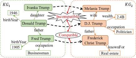
Figure 1: Example of EA predictions. While different mappings have dependencies, the neural EA model may make incompatible predictions.

Neural EA models are the current state-of-the-art for entity alignment Sun et al. (2020b); Zhao et al. (2022); Zhang et al. (2020); Mao et al. (2021b) These methods use pre-aligned mappings to learn an EA model: it encodes entities into informative embeddings and then, for each source entity, selects the closest target entity in the vector space as its counterpart. Though significant progress has been achieved, the dependencies between entities, which is the nature of graph data, is under-explored. In an EA task, the counterparts of different entities within one KG should be compatible w.r.t. the underlying dependencies. For example, in Fig 1, the two mappings $\textit{Donald Trump}\equiv\textit{D.J. Trump}$ and $\textit{Ivanka Trump}\equiv\textit{Melania Trump}$ should not co-exist at the same time (i.e. they are incompatible) since "someone’s daughter and wife cannot be the same person". On the contrary, $\textit{Donald Trump}\equiv\textit{D.J. Trump}$ and $\textit{Fred Trump}\equiv\textit{Frederick Christ Trump}$ are compatible mappings since equivalent entities’ father entities should also be equivalent. Through an experimental study, we verified that more effective EA models make more compatible predictions (see Appendix A for more details). Therefore, we argue that making compatible predictions should be one of the objectives of training a neural EA model, other than fitting the labelled data. Unfortunately, compatibility has thus far been neglected by the existing neural EA works.

To fill this gap, we propose a training framework EMEA , which exploits compatibility to improve existing neural EA models. Few critical problems make it challenging to drive a neural EA model with compatibility: (1) A first problem is how to measure the overall compatibility of all EA predictions. We notice some reasoning rules defined in traditional reasoning-based EA works Suchanek et al. (2011) can reflect the dependencies between entities well. To inherit their merits, we devise a compatibility model which can reuse them. In this way, we contribute one mechanism of combining reasoning-based and neural EA methods. (2) The second problem is how to improve the compatibility of EA model. Compatibility is measured on the counterparts (i.e. labels) sampled from the EA model, but the sampling process is not differentiable and thus the popular approach of regularizing an item in the loss is infeasible. We overcome this problem with variational inference. (3) The third problem lies in optimising the compatibility model, which has interdependencies with the unknown counterparts. We solve this problem with a variational EM framework, which alternates updating the neural EA model and the compatibility model until convergence.

Our contributions can be summarized as:

• We investigate the compatibility issue of the neural EA model, which is critical but so far neglected by the existing neural EA works.

• We propose one generic framework, which can guide the training of neural EA models with compatibility apart from labelled data.

• Our framework bridges the gap between neural and reasoning-based EA methods.

• We empirically show compatibility is very powerful in improving neural EA models, especially when the training data is limited .

2 Related Work

Neural EA. Entity Alignment is an important task and has been widely studied. Neural EA Sun et al. (2020b); Zhao et al. (2022); Zhang et al. (2020) is current mainstream direction which emerges with the development of deep learning techniques. Various neural architectures have been introduced to encode entities. Translation-based KG encoders were explored at the start Chen et al. (2017); Zhu et al. (2017). Though these models could capture the structure information, they were not capable of incorporating attribute information. Graph Convolutional Network (GCN)-based encoders later became the mainstream method because they were flexible in combining different types of information and achieved higher performance Wang et al. (2018); Cao et al. (2019); Mao et al. (2020a); Sun et al. (2020a); Mao et al. (2020b). Neural EA models rely on pre-aligned mappings for training Liu et al. (2021a). To improve EA effectiveness, semi-supervised learning (self-training) was explored to generate pseudo mappings to enrich the training data Sun et al. (2018); Mao et al. (2021b). Our work aims to complement the existing EA works regardless of their training methods.

Among previous neural EA methods, some were done on KGs with rich attributes and pay attention to exploiting extra information other than KG structure Wu et al. (2019); Liu et al. (2021b, 2020); Mao et al. (2021c); Qi et al. (2021). Alternatively, some others only focused on designing novel models to extract better features from the KG structure Sun et al. (2018, 2020a); Mao et al. (2020b); Liu et al. (2022) since structure is the most basic information and the proposed method would be more generic. We evaluate our method by applying it to models that only consider KG structure, which is a more challenging setting.

Reasoning-based EA. In the reasoning-based EA works Saïs et al. (2007); Hogan et al. (2007); Suchanek et al. (2011), some rules are defined based on the dependencies between entities. With the rules, label-level reasoning, i.e. inferring the label of one entity according to other entities’ labels instead of its own features, was performed to detect more potential mappings from the pre-aligned ones. Functional relation (or attribute), which can only have one object for a certain subject, is critical for some reasoning rules Hogan et al. (2007). One rule example is: $\exists r,e_{1},e^{\prime}_{1}:r(e_{1},r,e_{2}),r(e^{\prime}_{1},r,e^{\prime}_{2}),r\textit{ is functional},e_{1}\equiv e^{\prime}_{1}\Rightarrow e_{2}\equiv e^{\prime}_{2}$. Saïs et al. proposed to combine multiple properties instead of only using a functional property since the combination of several weak properties can also be functional. Hogan et al. quantified functional as functionality in a statistical way. Suchanek et al. inherited the reasoning ideas from previous works and further transformed the logic rules into a probabilistic form in their work named PARIS. Apart from Suchanek et al. (2011), few recent works Sun et al. (2020b); Zhao et al. (2022) verified PARIS can achieve promising performance. In this work, we reuse one reasoning rule defined in PARIS because it is very effective and representative.

Combining Reasoning-based and Neural EA. One previous work named PRASE Qi et al. (2021) also explored the combination of neural and reasoning-based EA methods. It used a neural EA model to measure the similarities between entities and fed these similarities to the reasoning method of PARIS. Our work provides a different combination mechanism of these two lines of methods.

3 Notations & Problem Definition

Suppose we have two KGs $\mathcal{G}$ and $\mathcal{G}^{\prime}$ with respective entity sets $E$ and $E^{\prime}$. Each source entity $\mathrm{e}\in E$ corresponds to one counterpart variable $y_{e}\in E^{\prime}$. For simplicity, we denote the counterpart variables of a set $E$ of entities as $y_{E}$ collectively, while use $\hat{y}_{e}$ to represent an assignment of $y_{e}$. The counterpart variables $y_{L}$ of labelled entities $L\subset E$ are already known (i.e. $\hat{y}_{L}$). EA aims to solve the unknown variables $y_{U}$ of the unlabelled entities $U\subset E$.

One neural EA model measures the similarity $s_{\Theta}(e,e^{\prime})$ between each source entity $e\in E$ and each target entity $e^{\prime}\in E^{\prime}$, and infers its counterpart via $\hat{y}_{e}=\arg\max_{e^{\prime}\in E^{\prime}}s_{\Theta}(e,e^{\prime})$. Here, $\Theta$ represents the parameters of the EA model.

4 The EMEA Framework

Fig. 2 shows an overview of our EMEA framework. Towards improving a given neural EA model, the EMEA performs the following core operations:

(1) Normalises similarities between source entity $e$ and all target entities into distribution $q_{\Theta}(y_{e})$;

(2) Measure the compatibility of all predictions by modelling the joint probability $p_{\Phi}(y_{L},y_{U})$ ($\Phi$ is paramters) of all (known or predicted) mappings;

(3) Derive more compatible predictions $q^{*}(y_{U})$ (than current EA model) using the compatibility model to guide updating the EA model.

(4) To learn the parameters of the compatibility model, we devise one optimisation mechanism based on variational EM Neal and Hinton (1998), which alternates the update of $\Theta$ and $\Phi$. The neural EA model $\Theta$ is initially trained in its original way. In the M-step, we assume current $\Theta$ is correct, and sample $\hat{y}_{U}\sim q_{\Theta}$ to update $\Phi$. In the E-step, we in turn assume current $\Phi$ is correct, and exploit $p_{\Phi}$ to derive more compatible distribution $q^{*}(y_{u})$. The neural EA model $\Theta$ is then updated using the samples $\hat{y}_{U}\sim q^{*}$ together with the labelled data. This EM process repeats until $\Theta$ converges.

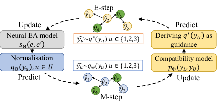
Figure 2: Overview of the EMEA framework. The two modules are trained iteratively with variational EM.

4.1 Normalising EA Similarity to Probability

Our method relies on the distribution form of counterpart variable $y_{e}$ as will be seen. However, the existing neural EA models only output similarities. To solve this problem, we introduce a separate model to normalise the similarities into probabilities . Given entity $e\in E$ and similarities $s_{\Theta}(e,e^{\prime})$, we use $s(e,e^{\prime})=s_{\Theta}(e,e^{\prime})$ and $d(e,e^{\prime})=\max\left(s_{\Theta}(e,:)\right)-s_{\Theta}(e,e^{\prime})$ as features of each target entity $e^{\prime}\in E^{\prime}$. These features are combined linearly and fed into a softmax function with a temperature factor $\tau$, as shown in Eq. 1 and 2. The parameters $\Omega=\{\omega_{1},\omega_{2},\omega_{0},\tau\}$ are learned by minimizing cross-entropy loss on the labelled data, i.e. Eq. 3. With the obtained model, we can transform $s_{\Theta}(e,e^{\prime})$ into $q_{\Theta}(y_{e})$.

$$f(e,e^{\prime})=\omega_{1}\cdot s(e,e^{\prime})+\omega_{2}\cdot d(e,e^{\prime})+\omega_{0}$$ (1)

$$\mathrm{Pr}_{\Omega}(y_{e}=e^{\prime})=\frac{\exp(f_{\Theta}(e,e^{\prime})/\tau)}{\mathrm{sum}\left(\exp(f_{\Theta}(e,:)/\tau)\right)}$$ (2)

$$O_{\Omega}=-\sum_{e\in L}\log\mathrm{Pr}_{\Omega}(y_{e}=\hat{y}_{e})$$ (3)

4.2 Measuring Compatibility

It is not easy to establish the distribution $p_{\Phi}(y_{L},y_{U})$ over a large number of variables $y_{L},y_{U}$. To address this problem, we model $p_{\Phi}(y_{L},y_{U})$ with graphical model Wainwright and Jordan (2008); Bishop (2006), which can be represented by a product of local functions (i.e. local compatibility). Each local function only depends on a factor subset  $F\subset E$, which is small and can be checked easily.

4.2.1 Local Compatibility

One rule $\kappa$ is defined on a set of labels $y_{F}$ according to the potential dependencies among $y_{F}$. The assignments of variables $y_{F}$ meeting the rule $\kappa$ are thought compatible. Given a rule set $\mathcal{K}=\{\kappa_{1},\kappa_{2},...,\kappa_{|\mathcal{K}|}\}$ and a factor subset $F$ to check, we define the corresponding local compatibility (i.e. local function) as Eq. 4, where $g_{\kappa}(\cdot)$ is an indicator function, $\Phi=\{\phi_{\kappa\in\mathcal{K}},\phi_{0}\}$ are the weights of rules.

$$l(y_{F})=\exp\left(\sum_{\kappa\in\mathcal{K}}\phi_{\kappa}\cdot g_{\kappa}(y_{F})+\phi_{0}\right)$$ (4)

Next, we use two concrete examples to explain local compatibility. The PARIS rule is the primary one used by our framework, while another is for exploring the generality of different rule sets.

PARIS Rule

Suchanek et al. (2011) can be understood intuitively as: one mapping $y_{e}=e^{\prime}$ can be inferred from (or supported by) the other mappings between their neighbours $\mathcal{N}_{e}$ and $\mathcal{N}_{e^{\prime}}$.

Given the predicted mappings, we can build one factor subset $F_{e}$ at each entity $e$, which contains $e$ and its neighbouring entities $\mathcal{N}_{e}$. Then, we check whether PARIS rule can be satisfied by mappings $y_{F_{e}}$. For example, in Fig. 3, we want to check the PARIS compatibility at $e_{2}$. In plot (a), for the mapping $y_{2}=e^{\prime}_{2}$ we can find two mappings between the neighbours of $e_{2}$ and $e^{\prime}_{2}$ – $y_{1}=e^{\prime}_{1}$ and $y_{3}=e^{\prime}_{3}$. Also, they can provide supporting evidence for $y_{2}=e^{\prime}_{2}$: if two entities have equivalent father entities and equivalent friend entities, they might also be equivalent. However, in plot (b), $y_{2}=e^{\prime}_{4}$ cannot get this kind of supporting evidence since there is no mapping between the neighbours of $e_{2}$ and $e^{\prime}_{4}$. Thus, the local PARIS compatibility at $e_{2}$ in plot (a) is higher than that in plot (b).

In this work, we reuse the probabilistic form of PARIS rule (i.e. Eq.(13) in Suchanek et al. (2011)) as our indicator function $g$. See Appendix B.5 for its equation with our symbols.

Figure 3: Example of PARIS compatibility. In (a), $y_{2}=e^{\prime}_{2}$ can get supporting evidence from $y_{1}=e^{\prime}_{1}$ and $y_{3}=e^{\prime}_{3}$, while $y_{2}=e^{\prime}_{4}$ in (b) cannot. Thus, the compatibility at $e_{2}$ in (a) is higher than that in (b).

Rules for Avoiding Conflicts.

We notice that most neural EA works assume that there is no duplicate within one KG, and thus different entities should have different counterparts. Otherwise, EA model makes conflicting predictions for them.

To reduce alignment conflicts, at each entity $e$, we build one factor subset $F_{e}$, which includes $e$ and its top-$N$ nearest neighbours in the embedding space of EA model. Basically, $y_{e}$ should follow the prediction of neural EA model, i.e. $g_{1}(y_{F_{e}})=\mathbbm{1}_{y_{e}=\arg\max_{e^{\prime}\in E}s_{\Theta}(e,e^{\prime})}$; Further, $y_{e}$ should be unique, i.e. $g_{2}(y_{F_{e}})=\mathbbm{1}_{y_{e}\neq y_{n},\forall n\neq e}$.

4.2.2 Overall Compatibility

We further formulate the overall compatibility by aggregating local compatibilities on all the factor subsets $\mathcal{F}=\{F_{e},e\in E\}$ as in Eq. 5, where $z$ is for normalisation.

$$p_{\Phi}(y_{L},y_{U})=\frac{1}{z}\prod_{F\in\mathcal{F}}l(y_{F})$$ (5)

$$z=\sum_{y_{U}\in E^{|U|}}\prod_{F\in\mathcal{F}}l(y_{F})$$ (6)

Note that $z$ is intractable because it involves integral over $y_{U}\in E^{|U|}$, which is a very large space. For such computation reason, we avoid computing $p_{\Phi}(y_{L},y_{U})$, conditional probability like $p_{\Phi}(y_{U}|y_{L})$, and marginal probability $p_{\Phi}(y_{L})$ directly in the following sections.

Instead, we will exploit $p_{\Phi}(y_{e}|y_{-e})$ ($-e$ refers to $E\setminus e$), whose computation is actually much easier. As in Eq. 7, computing $p_{\Phi}(y_{e}|y_{-e})$ only involves a few factor subsets containing $e$. $\mathrm{MB}^{e}$ is the Markov Blanket of $e$, which only contains entities cooccuring in any factor subset with $e$. See Appendix B.1 for the derivation process.

$$p_{\Phi}(y_{e}|y_{-e}) =\frac{\prod_{F|e\in F}l(y_{F})}{\sum_{e^{\prime}\in E^{\prime}}\prod_{F|e\in F}l(y_{F}|y_{e}=e^{\prime})}$$ (7)

$$\doteq p_{\Phi}(y_{e}|y_{\mathrm{MB}^{e}})$$

4.3 Guiding Neural EA with Compatibility

Suppose we have $p_{\Phi}(y_{L},y_{U})$ which can measure the compatibility well. We attempt to make the distribution $q_{\Theta}(y_{U})$ close to $p_{\Phi}(y_{U}|y_{L})$, so that variable $y_{U}$ sampled from $q_{\Theta}$ are compatible. To this end, we treat minimizing the KL-divergence $\mathrm{KL}(q_{\Theta}(y_{U})||p_{\Phi}(y_{U}|y_{L}))$ as one of the objectives of optimising neural EA model $\Theta$.

However, it is difficult to minimize the KL-divergence directly. We solve this problem with variational inference Hogan (2002). As shown in Eq. 8 and 9, the KL-divergence can be written as the difference between observed evidence $\log p_{\Phi}(y_{L})$, which is irrelevant to $\Theta$, and its Evidence Lower Bound (ELBO), i.e. Eq. 9 (see Appendix B.2 for derivation process.). Minimizing the KL divergence is equivalent to maximizing the ELBO, which is computationally simpler.

$$\mathrm{KL}(q_{\Theta}(y_{U})||p_{\Phi}(y_{U}|y_{L}))=\log p_{\Phi}(y_{L})-\mathrm{ELBO}$$ (8)

$$\begin{split}\mathrm{ELBO}=&\mathbb{E}_{q_{\Theta}(y_{U})}\log p_{\Phi}(y_{U},y_{L})\\ &-\mathbb{E}_{q_{\Theta}(y_{U})}\log q_{\Theta}(y_{U})\end{split}$$ (9)

Because $y_{i}$ are independent in neural EA model, we have $q(y_{U})=\prod_{i\in U}q(y_{i})$. In addition, we use pseudolikelihood Besag (1975) to approximate the joint probability $p_{\Phi}(y_{U},y_{L})$ for simpler computation, as in Eq. 10. Then, ELBO can be approximated with Eq. 11 (see Appendix B.3 for derivation details), where $-u$ denotes $U\setminus u$.

$$p_{\Phi}(y_{U},y_{L}) =p_{\Phi}(y_{L})\prod_{u\in U}p_{\Phi}(y_{u}|y_{1:u-1},y_{L})$$ (10)

$$\approx p_{\Phi}(y_{L})\prod_{u\in U}p_{\Phi}(y_{u}|y_{-u})$$

$$\begin{split}O_{\Theta}=\sum_{u\in U}\mathbb{E}_{q_{\Theta}(y_{u})}\Big{[}\mathbb{E}_{q_{\Theta}({y_{-u}})}[\log p_{\Phi}(y_{u}|y_{-u})]\\ -\log q_{\Theta}(y_{u})\Big{]}\end{split}$$ (11)

Now, our goal becomes to maximize $O_{\Theta}$ w.r.t. $\Theta$. Our solution is to derive a local optima $q^{*}(y_{U})$ of $q_{\Theta}(y_{U})$ with coordinate ascent, and then exploit $\hat{y}_{U}\sim q^{*}(y_{U})$ to update $\Theta$. In particular, we initialize $q^{*}(y_{U})$ with current $q_{\Theta}(y_{U})$ firstly. Then, we update $q^{*}(y_{u})$ for each $u\in E$ in turn iteratively. Everytime we only update a single (or a block of) $q^{*}(y_{u})$ with Eq. 12, which can be derived from $\frac{dQ_{\Theta}}{dq_{\Theta}(y_{u})}=0$ (see Appendix B.4 for derivation details), while keeping the other $q^{*}(y_{-u})$ fixed. This process ends until $q^{*}(y_{U})$ converges.

$$q^{*}(y_{u})\propto\exp\left(\mathbb{E}_{q_{\Theta}(y_{\mathrm{MB}^{u}})}\log p_{\Phi}(y_{u}|y_{\mathrm{MB}^{u}})\right)$$ (12)

Afterwards, we sample $\hat{y}_{u}\sim q^{*}(y_{u})$ for $u\in U$, and join $\hat{y}_{U}$ with the labelled data $\hat{y}_{L}$ to form the training data. Eventually, we update $\Theta$ with the original training method of neural EA model.

4.4 Optimisation with Variational EM

Though we have derived a way of guiding the training of $\Theta$ with $p_{\Phi}$, it remains a problem to optimise the weights of rules $\Phi$. Typically, we learn $\Phi$ by maximizing the log-likelihood of observed data $\log p_{\Phi}(y_{L})$. However, as shown in $\log p_{\Phi}(y_{L})=\log\sum_{y_{U}}p_{\Phi}(y_{L},y_{U})$, $\log p_{\Phi}(y_{L})$ relies on the latent variables $y_{U}$. We apply a variational EM framework Neal and Hinton (1998); Qu and Tang (2019) to update $\Theta$ and $\Phi$ by turns iteratively. In E-step, we compute the expectation of $\log p_{\Phi}(y_{L},y_{U})$, i.e. $\mathbb{E}_{p_{\Phi}(y_{U}|y_{L})}\log p_{\Phi}(y_{L},y_{U})$. Here, we approximate $p_{\Phi}(y_{U}|y_{L})$ with $q_{\Theta}(y_{U})$ and use the pseudolikelihood to approximate $p_{\Phi}(y_{L},y_{U})$; Accordingly, we obtain the objective Eq. 13 for optimization. In M-step, we update $\Phi$ to maximize $O_{\Phi}$.

$$O_{\Phi} =\mathbb{E}_{q_{\Theta}(y_{U})}\log p_{\Phi}(y_{L},y_{U})$$ (13)

$$\approx\mathbb{E}_{q_{\Theta}(y_{U})}\sum_{e\in E}\log p_{\Phi}(y_{e}|y_{-e})$$

4.5 Implementation

1 Train neural EA model $\Theta$ using $\hat{y}_{L}$ ;

2 Normalise EA similarity to get $q_{\Theta}(y_{u})$ ;

3 for iterations do

       // M-step

4       Update $\Phi$ by maximizing Eq. 13 ;

       // E-step

5       Derive $q^{*}(y_{U})$ with Eq. 12 ;

6       Sample $\hat{y}_{u}\sim q^{*}(y_{u})$ for $u\in U$ ;

7       Update EA model $\Theta$ with data $\hat{y}_{U}\cup\hat{y}_{L}$ ;

8       Normalise EA similarity to get $q_{\Theta}(y_{u})$ ;

9      

Algorithm 1 The EMEA Framework

We take a few measures to simplify the computation. (1) In Eq. 12 and Eq. 13, it is costly to estimate distribution $q^{*}(y_{u})$ and $p_{\Phi}(y_{u})$ because $y_{u}$’s assignment space $E^{\prime}$ can be very large. Instead, we only estimate $q^{*}(y_{u})$ for the top $K$ most likely candidates according to current $q_{\Theta}(y_{u})$. (2) Both Eq. 11 and Eq. 12 involve sampling from $q_{\Theta}(y_{u})$ for estimating the expectation. We only sample one $y_{u}$ as in $\hat{y}_{u}=\arg\max_{e^{\prime}\in E}q_{\Theta}(y_{u}=e^{\prime})$ for each $u\in U$. (3) When computing $q^{*}(y_{U})$ with coordinate ascent, we treat $U$ as a single block and update $q^{*}(y_{U})$ for once.

We describe the whole process of EMEA in Alg. 1.

5 Experimental Settings

5.1 Datasets and Partitions

We choose five datasets widely used in previous EA research. Each dataset contains two KGs and a set of pre-aligned entity mappings. Three datasets are from DBP15K Sun et al. (2017), which contains three cross-lingual KGs extracted from DBpedia: French-English (fr_en), Chinese-English (zh_en), and Japanese-English (ja_en). Each KG contains around 20K entities, among which 15K are pre-aligned. The other two datasets are from DWY100K Sun et al. (2018), which consists of two mono-lingual datasets: dbp_yg extracted from DBpedia and Yago, and dbp_wd extracted from DBpedia and Wikidata. Each KG contains 100K entities which are all pre-aligned. Our experiment settings only consider the structural information of KGs and thus will not be affected by the problems of attributes like name bias in these datasets Zhao et al. (2022); Liu et al. (2020).

Most existing EA works use 30% of the pre-aligned mappings as training data, which however was pointed out unrealistic in practice Zhang et al. (2020). We explore the power of compatibility under different amounts of labelled data – 1%, 5%, 10%, 20%, and 30% of pre-aligned mappings, which are sampled randomly. Another 100 mappings are used as the validation set, while all the remaining mappings form the test set.

Table 1: Overall performance of EMEA and PRASE in combining RREA (sup) and PARIS rule across different percentages (1%-30%) of annotations. Bold indicates best for the specific annotation percentage; all differences between RREA and other baselines are statistically significant ($p<0.01$); the hyphen ’-’ means not applicable because the corresponding methods do not formulate EA as a ranking problem. The results of PRASE and PARIS have big differences from those in the literature because of different experimental settings.

	Method	zh_en			fr_en			ja_en			dbp_wd			dbp_yg
		Hit@1	MRR	MR	Hit@1	MRR	MR	Hit@1	MRR	MR	Hit@1	MRR	MR	Hit@1	MRR	MR
1%	PARIS	0.01	-	-	0.016	-	-	0.002	-	-	0.19	-	-	0.451	-	-
	RREA (sup)	0.140	0.215	652.3	0.126	0.208	366.5	0.138	0.203	684.0	0.278	0.368	317.9	0.509	0.602	64.4
2-17	PRASE	0.241	-	-	0.227	-	-	0.163	-	-	0.517	-	-	0.667	-	-
	EMEA	0.517	0.591	116.4	0.480	0.565	72.1	0.411	0.488	181.3	0.581	0.657	72.8	0.773	0.828	17.6
5%	PARIS	0.221	-	-	0.281	-	-	0.226	-	-	0.537	-	-	0.608	-	-
	RREA (sup)	0.413	0.518	118.8	0.424	0.539	65.3	0.391	0.496	113.9	0.522	0.616	78.4	0.737	0.803	21.0
2-17	PRASE	0.461	-	-	0.514	-	-	0.432	-	-	0.531	-	-	0.689	-	-
	EMEA	0.665	0.738	36.8	0.677	0.757	18.0	0.630	0.710	35.9	0.708	0.778	21.5	0.811	0.861	12.7
10%	PARIS	0.414	-	-	0.473	-	-	0.395	-	-	0.623	-	-	0.64	-	-
	RREA (sup)	0.542	0.641	56.9	0.571	0.675	31.3	0.528	0.631	52.6	0.622	0.709	36.2	0.782	0.841	14.0
2-17	PRASE	0.522	-	-	0.575	-	-	0.508	-	-	0.679	-	-	0.701	-	-
	EMEA	0.706	0.777	27.4	0.727	0.802	9.7	0.688	0.764	24.5	0.755	0.820	13.4	0.828	0.877	9.2
20%	PARIS	0.532	-	-	0.584	-	-	0.511	-	-	0.69	-	-	0.676	-	-
	RREA (sup)	0.657	0.745	26.5	0.686	0.775	14.7	0.649	0.740	25.3	0.711	0.787	20.6	0.824	0.875	12.0
2-17	PRASE	0.593	-	-	0.622	-	-	0.580	-	-	0.726	-	-	0.719	-	-
	EMEA	0.748	0.815	16.6	0.773	0.841	6.8	0.736	0.807	16.3	0.808	0.866	6.6	0.846	0.891	10.4
30%	PARIS	0.589	-	-	0.628	-	-	0.577	-	-	0.739	-	-	0.696	-	-
	RREA (sup)	0.720	0.797	16.7	0.742	0.821	9.2	0.717	0.797	14.9	0.758	0.827	14.0	0.849	0.894	6.9
2-17	PRASE	0.623	-	-	0.649	-	-	0.613	-	-	0.754	-	-	0.735	-	-
	EMEA	0.782	0.842	12.6	0.801	0.863	5.9	0.771	0.837	12.6	0.836	0.889	7.3	0.862	0.904	5.8

5.2 Metrics

EA methods typically output a ranked list of candidate counterparts for each entity. Therefore, we choose metrics for measuring the quality of ranking. We use Hit@1 (i.e., accuracy), Mean Reciprocal Rank (MRR) and Mean Rank (MR) to reflect the model performance at suggesting a single entity, a handful of entities, and many entities. Higher Hit@1, higher MRR, and lower MR indicate better performance. Statistical significance is performed using paired two-tailed t-test.

5.3 Comparable Methods

Baselines. We select baselines with the following considerations: (1) To examine the effect of compatibility, we compare EMEA with the original neural EA model. (2) We compare EMEA with PARIS, which performs reasoning with the rule, to gain insights on different ways of using the rules. (3) To compare different combination mechanisms of neural and reasoning-based EA methods, we add PRASE Qi et al. (2021), which exploits neural models to improve PARIS Suchanek et al. (2011), as one baseline.

Neural EA models. For our choice of neural models, we select RREA Mao et al. (2020b), which is a SOTA neural EA model under both supervised (denoted as RREA (sup)) and semi-supervised (denoted as RREA (semi)) modes. In addition, we also choose Dual-AMN Mao et al. (2021b), AliNet Sun et al. (2020a) and IPTransE Zhu et al. (2017) to verify the generality of EMEA across different neural models. These three neural models vary in performance (see Appendix C.1) and KG encoders.

Note direct comparison between EMEA and the existing neural EA methods is not fair. The EMEA is a training framework designed to enhance the existing neural EA models. Its effectiveness is reflected by the performance difference of neural EA models before and after being enhanced with EMEA . The details about reproducibility (e.g. hyperparameter settings, etc.) can be found in Appendix C.

6 Results

Comparison with Baselines

In Table 1, we report the overall performance of EMEA with supervised RREA and the baselines. Note the results of PRASE and PARIS are much lower than those in the literature because we only use the structure information of KGs for all the methods. We have the following findings:

(1) By comparing EMEA with RREA, we can see that EMEA can significantly improve RREA across all the datasets and percentages of labelled data, especially when the amount of labelled data is small. For instance, EMEA using 5% of labelled data can achieve comparable effectiveness with supervised RREA using 20% of labelled data.

(2) EMEA always outperforms PARIS with a big margin. Thus, EMEA provides a better way of using the same reasoning rule. PARIS can only do label-level inference based on the reasoning rule, while EMEA can combine the power of neural EA model and reasoning rule.

(3) Some existing works show PARIS have very competitive performance with the SOTA neural EA models when the attribute information can be used. However, we find its performance is actually much worse than the SOTA neural model RREA when only the KG structure is available. This is a complementary finding about PARIS to the literature.

(4) Regarding the combination of RREA and PARIS, EMEA outperforms PRASE across all datasets and annotation costs. Though PRASE can always improve PARIS, there are some cases where it is worse than only using RREA. The potential reason is PARIS becomes the bottleneck of PRASE. On the contrary, EMEA is more robust – it consistently performs better than separately running RREA or PARIS.

To conclude, EMEA can significantly improve the SOTA EA model RREA by introducing compatibility. It also provides an effective combination mechanism of neural and reasoning-based EA methods, which outperforms the existing methods.

The further explorations of EMEA are done on zh_en dataset if not specially clarified.

Table 2: Overall performance of EMEA in combining RREA (semi) with PARIS rule across different percentages (1%-30%) of annotations. Bold indicates best for the specific annotation percentage; all differences between RREA and EMEA are statistically significant ($p<0.05$).

	Method	zh_en		fr_en		ja_en
		Hit@1	MRR	Hit@1	MRR	Hit@1	MRR
1%	RREA (semi)	0.309	0.405	0.277	0.382	0.263	0.348
	EMEA	0.471	0.541	0.435	0.518	0.386	0.457
5%	RREA (semi)	0.590	0.683	0.610	0.708	0.550	0.647
	EMEA	0.680	0.751	0.703	0.778	0.641	0.716
10%	RREA (semi)	0.677	0.757	0.710	0.791	0.658	0.743
	EMEA	0.731	0.796	0.762	0.828	0.711	0.781
20%	RREA (semi)	0.756	0.821	0.782	0.848	0.743	0.814
	EMEA	0.782	0.840	0.805	0.865	0.765	0.829
30%	RREA (semi)	0.794	0.851	0.819	0.876	0.790	0.851
	EMEA	0.808	0.862	0.833	0.886	0.801	0.859

Generality across Neural EA Models

To explore the generality of EMEA across neural EA models, we apply EMEA to another three models: Dual-AMN Mao et al. (2021b), AliNet Sun et al. (2020a) and IPTransE Zhu et al. (2017) other than RREA. We find that: (1) EMEA can bring improvements to the three EA models as shown in Fig.4 (a), (b) and (c). Also, no matter whether the neural model is better or worse than PARIS, their combination using EMEA is more effective than using them separately. (2) Fig.4 (d) shows more effective neural models lead to more accurate final results.

Generality across Training Modes

To verify the generality of EMEA across training modes, we also attempt to apply EMEA to improve semi-supervised RREA. As reported in Table 2, we find that EMEA can also boost semi-supervised RREA consistently across different datasets and amounts of training data. By comparing EMEA in Table 1 and Table 2, we find that semi-supervised RREA usually leads to better final EA effectiveness than supervised RREA after the boost of EMEA . Nevertheless, when the training data is extremely small, i.e. 1%, semi-supervised RREA get worse final EA effectiveness than the supervised one. This might be caused by the low-quality seeds iteratively added into the training data during the semi-supervised training. We treat the exploration of this phenomenon as future work.

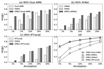
Figure 4: Generality of EMEA on neural EA models. Plots (a), (b) and (c) show EMEA can boost different EA models consistently; Plot (d) shows better EA models lead to a better final performance.

7 Further Analysis

Further analysis of EMEA is done on dataset zh_en.

Impact of Compatibility on Training Process

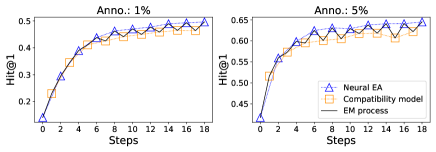
Figure 5: Convergence process of EMEA trained with 1% and 5% annotations. Compatibility model can boost the neural EA model, no matter whether it can derive more accurate supervision signals or not.

In each iteration of the training procedure, the compatibility model derives more compatible predictions to assist in updating the neural EA model in the next iteration. To gain insights into their interaction, we examine the EA effectiveness of the two components in the training process. Fig. 5 shows this processes running on datasets with 1% and 5% annotated data. Step 0 is the original neural EA model. We make the following observations: (1) Overall, the effectiveness of the two components jointly increases across the training procedure. This phenomenon indicates that they indeed both benefit from each other. (2) The compatibility model performs better than the neural model in the early stage while worse later. Thus, we can conclude that the compatibility model can always boost the neural EA model, regardless of whether it can derive more accurate supervision signals.

Effect of Rule Sets on EMEA

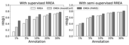
Figure 6: Effect of different rule sets on EMEA. PARIS rule is stronger than AvoidConf.

To explore the effect of different rule sets on EMEA , we deploy another rule set used for avoiding conflicts (denoted as AvoidConf here) in EMEA . As shown in Fig. 6, AvoidConf can improve supervised RREA consistently, as well as semi-supervised RREA when the training data is of a small amount. However, it can only bring very slight (or even no) improvement to the semi-supervised RREA when the training data is $>10\%$. Also, its performance is always worse than PARIS rule. Therefore, PARIS rule is stronger in indicating the compatibility of EA than AvoidConf. This finding is intuitively reasonable because the PARIS rule can be used to infer new mappings, while AvoidConf can only indicate the potential errors.

Sensitivity to Hyper-parameters

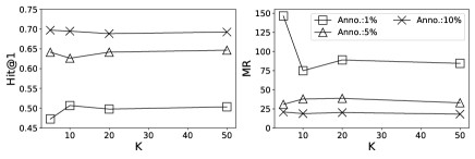
Figure 7: Sensitivity of EMEA to the parameter $K$ w.r.t. both shallow and deep metrics. The EMEA is not sensitive when $K$ is not too small; The poorer EA model (trained with fewer data) is relatively more sensitive; A small $K$ out of the sensitive range is suggested for the trade-off between computation cost and EA effectiveness.

We also analyse the sensitivity of parameter $K$ (discussed in Sec. 4.5) in EMEA under three annotation settings: 1%, 5% and 10%. Fig. 7 shows the performance of EMEA, measured with Hit@1 and MR, with respect to different $K$ values. We find that: (1) the performance of EMEA fluctuates when $K<10$ but is relatively stable when $K>10$. (2) EMEA is more sensitive to $K$ in settings with fewer annotations. The reason is that a well-trained neural model can rank most true correspondences in the top positions and thus is less affected by the cut-off. (3) Large $K$ values (e.g., 50) only make EMEA slightly more effective (note lower MR is better). Since larger $K$ values require more computation, a small value outside the sensitive range is suggested, like 10 in Fig. 7.

8 Conclusion

Entity Alignment is a primary step of fusing different Knowledge Graphs. Many neural EA models have been explored and achieved SOTA performance. Though, one nature of graph data – the dependencies between entities – is under-explored. In this work, we raise attention to one neglected aspect of EA task – different entities have compatible counterparts w.r.t. their underlying dependencies. We argue that making self-consistent predictions should be one objective of training EA model other than fitting the labelled data. Towards this goal, we devise one training framework named EMEA , which can intervene in the update of EA model to improve its compatibility. In EMEA , we address three key problems: (1) measure compatibility with a graphical model which can aggregate local compatibilities; (2) guide the training of EA models with the compatibility measure via variational inference; (3) optimize the compatibility module with a variational EM framework. We empirically show that compatibility is very powerful in driving the training of neural EA models. The EMEA complements the existing neural EA works.

Limitations

Our EMEA framework has a higher computation cost than the original neural EA model. It needs to compute the compatibility module and continue updating the neural EA model in the iterations. As a result, more time is taken to train the neural EA model. In addition, we only measure compatibility in one direction (i.e. selecting one KG as the source KG and measuring compatibility on the target KG). Considering both directions might be able to further increase the EA performance.

In future, we plan to explore dual compatibility modules. Also, we will study how to combine compatibility and self-training.

Appendix A Preliminary Study

Our preliminary study examines the compatibilities of neural EA models with different performances. We choose RREA Mao et al. (2020b) as the neural EA model and train it with different amounts of labelled data. As for the compatibility, we measure it with PARIS rule and the number of conflicting predictions (see Sec. 4.2). The PARIS compatibility is shown in Fig. 8, where the violins represent the distributions of compatibility scores while the triangles represent the average compatibilities. We can observe that RREA always makes numerous incompatible predictions, especially when trained with few annotated entities, while most oracle alignments are compatible. The curve strongly suggests that a better model makes more compatible predictions. Similar findings can be observed in Fig. 8 (b), where fewer conflicts mean better compatibility. These observations motivate us to improve the neural EA methods by guiding them to better compatibility.

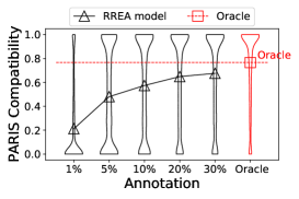
(a) PARIS compatibility.

(b) Conflicting prediction.

Figure 8: PARIS compatibility and proportions of conflicting predictions of RREA trained with different proportions of annotated data. Both plots highlight the correlation between compatibility and performance in EA models.

Appendix B Derivation Processes

B.1 Simplification of $p_{\Phi}(y_{e}|y_{-e})$

The derivation process of Eq. 7 is shown in Eq. 14. $\mathrm{MB}^{e}$ is the Markov Blanket of $e$ and only contains entities cooccuring in any factor subset with $e$. We only need to sample $y_{\mathrm{MB}^{e}}$ to compute $p_{\Phi}(y_{e}|y_{-e})$.

$$p_{\Phi}(y_{e}|y_{-e}) =\frac{p_{\Phi}(y_{e},y_{-e})}{p_{\Phi}(y_{-e})}=\frac{p_{\Phi}(y_{e},y_{-e})}{\sum_{e^{\prime}\in E^{\prime}}p_{\Phi}(y_{e}=e^{\prime},y_{-e})}$$ (14)

$$=\frac{\prod_{F|e\in F}\Phi(y_{F})\times\prod_{F|e\notin F}\Phi(y_{F})}{\sum_{e^{\prime}\in E^{\prime}}\prod_{F|e\in F}\Phi(y_{F}|y_{e}=e^{\prime})\times\prod_{F|e\in F}\Phi(y_{F})}$$

$$=\frac{\prod_{F|e\in F}\Phi(y_{F})}{\sum_{e^{\prime}\in E^{\prime}}\prod_{F|e\in F}\Phi(y_{F}|y_{e}=e^{\prime})}\doteq p_{\Phi}(y_{e}|y_{\mathrm{MB}^{e}})$$

B.2 Evidence Lower Bound

The relationship between KL divergence and ELBO shown in Eq. 8 and Eq. 9 can be derived through Eq. 15.

$$\begin{split}\mathrm{KL}(q_{\Theta}(y_{U})||p_{\Phi}(y_{U}|y_{L}))&=\mathbb{E}_{q_{\Theta}(y_{U})}\log\frac{q_{\Theta}(y_{U})}{p_{\Phi}(y_{U}|y_{L})}\\ &=\mathbb{E}_{q_{\Theta}(y_{U})}\log q_{\Theta}(y_{U})-\mathbb{E}_{q_{\Theta}(y_{U})}\log p_{\Phi}(y_{U}|y_{L})\\ &=\mathbb{E}_{q_{\Theta}(y_{U})}\log q_{\Theta}(y_{U})-\mathbb{E}_{q_{\Theta}(y_{U})}\log p_{\Phi}(y_{U},y_{L})+\mathbb{E}_{q_{\Theta}(y_{U})}\log p_{\Phi}(y_{L})\\ &=-\left(\mathbb{E}_{q_{\Theta}(y_{U})}\log p_{\Phi}(y_{U},y_{L})-\mathbb{E}_{q_{\Theta}(y_{U})}\log q_{\Theta}(y_{U})\right)+\log p_{\Phi}(y_{L})\end{split}$$ (15)

B.3 Derivation of $Q_{\Theta}$

The ELBO can be written as in Eq. 16. In the last line, the first item is irrelevant to $\Theta$. Thus, we drop it and keep the second item as $Q_{\Theta}$.

$$\begin{split}\mathrm{ELBO}&=\mathbb{E}_{q_{\Theta}(y_{U})}\log p_{\Phi}(y_{U},y_{L})-\mathbb{E}_{q_{\Theta}(y_{U})}\log q_{\Theta}(y_{U})\\ &\approx\mathbb{E}_{q_{\Theta}(y_{U})}\log(p_{\Phi}(y_{L})\prod_{u\in U}p_{\Phi}(y_{u}|y_{-u},y_{L}))-\mathbb{E}_{q_{\Theta}(y_{U})}\log\prod_{u\in U}q_{\Theta}(y_{u})\\ &=\mathbb{E}_{q_{\Theta}(y_{U})}\log p_{\Phi}(y_{L})+\mathbb{E}_{q_{\Theta}(y_{U})}\sum_{i\in U}\log p_{\Phi}(y_{u}|y_{-u},y_{L})-\mathbb{E}_{q_{\Theta}(y_{U})}\sum_{u\in U}\log q_{\Theta}(y_{u})\\ &=\log p_{\Phi}(y_{L})+\sum_{u\in U}\left(\mathbb{E}_{q_{\Theta}(y_{u})}[\mathbb{E}_{q_{\Theta}(y_{-u})}\log p_{\Phi}(y_{u}|y_{-u},y_{L})]-\mathbb{E}_{q_{\Theta}(y_{u})}\log q_{\Theta}(y_{u})\right)\\ &=\log p_{\Phi}(y_{L})+\sum_{u\in U}\left(\mathbb{E}_{q_{\Theta}(y_{u})}[\mathbb{E}_{q_{\Theta}(y_{-u})}\log p_{\Phi}(y_{u}|y_{-u},y_{L})-\log q_{\Theta}(y_{u})]\right)\end{split}$$ (16)

B.4 Derivation of $q^{*}$

We write $Q_{\Theta}$ in the form of Eq. 17, and then differentiate ${Q_{\Theta}}$ regarding $q_{\Theta}(y_{u})$ as in Eq. 18. By letting $\frac{dQ_{\Theta}}{dq_{\Theta}(y_{u})}=0$, we can get Eq. 12. Note that the obtained $q^{*}$ in Eq. 12 needs to be normalized into probabilities since it is proportional to (i.e. $\propto$) the right size, which is not normalized.

$$Q_{\Theta}=\sum_{u\in U}\sum_{y_{u}}q_{\Theta}(y_{u})\left(\mathbb{E}_{q_{\Theta}(y_{-u})}\log p_{\Phi}(y_{u}|y_{-u},y_{L})-\log q_{\Theta}(y_{u})\right)$$ (17)

$$\frac{dQ_{\Theta}}{dq_{\Theta}(y_{u})} =\left(\mathbb{E}_{q_{\Theta}(y_{-u})}\log p_{\Phi}(y_{u}|y_{-u},y_{L})-\log q_{\Theta}(y_{u})\right)+q_{\Theta}(y_{u})(-\frac{1}{q_{\Theta}(y_{u})})$$ (18)

$$=\mathbb{E}_{q_{\Theta}(y_{-u})}\log p_{\Phi}(y_{u}|y_{-u},y_{L})-\log q_{\Theta}(y_{u})-1$$

B.5 Indicator Function of PARIS Rule

With symbols used in this work, the probabilistic form of PARIS rule, i.e. our indicator function, can be written as Eq. 19, where $r(e,n)$ denote any triple with $e$ as head entity, $r^{\prime}(y_{e},n^{\prime})$ denote any triple with $y_{e}$ as head entity. In addition, $\Pr(r^{\prime}\subseteq r)$ represents the likelihood that $r^{\prime}$ is a subrelation of $r$ ($\Pr(r\subseteq r^{\prime})$ is analogous), while $fun^{-1}(r)$ denotes the reverse functionality of relation $r$. See Suchanek et al. (2011) for more details about them.

$$g(y_{F_{e}})=\Pr(e\equiv y_{e})=1-\prod_{\begin{subarray}{c}r(e,n),r^{\prime}(y_{e},n^{\prime})\end{subarray}}$$ (19)

$$\left(1-\Pr(r^{\prime}\subseteq r)\times fun^{-1}(r)\times q_{\Theta}(y_{n}=n^{\prime})\right)\times$$

$$\left(1-\Pr(r\subseteq r^{\prime})\times fun^{-1}(r^{\prime})\times q_{\Theta}(y_{n}=n^{\prime})\right)$$

Appendix C Experiments

C.1 Performance of Neural EA Models

Table 3 summarizes the performance of SOTA neural EA models. The results of IPTransE, GCNAlign, MUGNN, RSN, AliNet are reported in Sun et al. (2020a) while others are reported in their original papers. The results of RREA trained with 30% of training data in Table 1 are reproduced by us and slightly different from the results reported in Table 3 because of different random settings. Similar situation can be found in Table 2.

Table 3: Performance of neural EA baselines. Percentage of labelled data: 30%; sup: supervised; semi: semi-supervised.

Method	zh_en		ja_en		fr_en
	Hit@1	MRR	Hit@1	MRR	Hit@1	MRR
IPTransE Zhu et al. (2017)	0.406	0.516	0.367	0.474	0.333	0.451
GCN-Align Wang et al. (2018)	0.413	0.549	0.399	0.546	0.373	0.532
MuGNN Cao et al. (2019)	0.494	0.611	0.501	0.621	0.495	0.621
RSN Guo et al. (2019)	0.508	0.591	0.507	0.590	0.516	0.605
AliNet Sun et al. (2020a)	0.539	0.628	0.549	0.645	0.552	0.657
MRAEA (sup) Mao et al. (2020a)	0.638	0.736	0.646	0.735	0.666	0.765
PSR (sup) Mao et al. (2021a)	0.702	0.781	0.698	0.782	0.731	0.807
RREA (sup) Mao et al. (2020b)	0.715	0.794	0.713	0.793	0.739	0.816
Dual-AMN (sup) Mao et al. (2021b)	0.731	0.799	0.726	0.799	0.756	0.827
BootEA (semi) Sun et al. (2018)	0.629	0.703	0.622	0.701	0.653	0.731
MRAEA (semi) Mao et al. (2020a)	0.757	0.827	0.758	0.826	0.781	0.849
PSR (semi) Mao et al. (2021a)	0.802	0.851	0.803	0.852	0.828	0.874
RREA (semi) Mao et al. (2020b)	0.801	0.857	0.802	0.858	0.827	0.881
Dual-AMN (semi) Mao et al. (2021b)	0.808	0.857	0.801	0.855	0.840	0.888

Table 4: Time consumption (seconds) of running EMEA on zh_en.

Anno.	Initialization	Neural Module	Joint Distr. Module
1 %	254.1	108.1$\pm$1.2	88.5$\pm$1.1
5 %	249.7	108.0$\pm$2.5	98.2$\pm$15.5
10 %	249.2	108.6$\pm$0.9	86.0$\pm$0.3
20 %	252.8	109.6$\pm$1.6	86.7$\pm$0.6
30 %	252.4	111.1$\pm$2.0	90.2$\pm$2.7

Table 5: Time consumption (minutes) of running EMEA on dbp_wd.

Anno.	Initialization	Neural Module	Joint Distr. Module
1 %	169.1	36.8$\pm$0.6	19.1$\pm$1.4
5 %	172.2	33.0$\pm$6.6	15.9$\pm$3.9
10 %	146.3	43.5$\pm$3.2	22.8$\pm$2.4
20 %	190.0	45.3$\pm$3.3	29.2$\pm$2.0
30 %	183.9	49.0$\pm$4.4	30.2$\pm$6.9

C.2 Details for Reproducibility

Hyper-parameters

We search the number of candidate counterparts $K$ from [5,10,20,50], and set it as 10 for the trade-off of effectiveness and efficiency as discussed in Sec. 7. The number of nearest neighbours $N$ in the AvoidConf rule is searched from [5,10,15,20] and set as 5 for similar consideration as $K$;

Implementation of Baselines and Neural EA Models

The source codes of PARIS  and PRASE  are used to produce their results. As for the neural EA models, RREA  and Dual-AMN  are implemented based on their source codes, while AliNet and IPTransE are implemented with OpenEA. . We use the default settings of their hyper-parameters in these source codes.

Configuration of Running Device

We run the experiments on one GPU server, which is configured with an Intel(R) Xeon(R) Gold 6128 3.40GHz CPU, 128GB memory, 3 NVIDIA GeForce GTX 2080Ti GPU and Ubuntu 20.04 OS.

C.3 Running Time

We report our running time on datasets zh_en (15K) and dbp_wd (100K) in Table 4 and 5 as reference. The experiments on other datasets take comparable running time as them w.r.t. corresponding dataset size. Note that these experiments are run on a shared server and cannot be used to measure the precise running efficiency. In each table, we count the time consumption of initializing EA model, updating EA model and computing the self-consistency module in each EM iteration. The experiments on dbp_wd (100K) are slow because the source code of RREA can only run on CPU while raising Out-of-Memory exception on GPU.

References

- Besag (1975) Julian Besag. 1975. Statistical analysis of non-lattice data. Journal of the Royal Statistical Society: Series D (The Statistician), 24(3):179–195.
- Bishop (2006) Christopher M Bishop. 2006. Chapter 8: Graphical models. Pattern Recognition and Machine Learning. Springer, pages 359–418.
- Cao et al. (2019) Yixin Cao, Zhiyuan Liu, Chengjiang Li, Zhiyuan Liu, Juanzi Li, and Tat-Seng Chua. 2019. Multi-channel graph neural network for entity alignment. In Proceedings of the 57th Conference of the Association for Computational Linguistics, ACL 2019, Florence, Italy, July 28- August 2, 2019, Volume 1: Long Papers, pages 1452–1461. Association for Computational Linguistics.
- Chen et al. (2017) Muhao Chen, Yingtao Tian, Mohan Yang, and Carlo Zaniolo. 2017. Multilingual knowledge graph embeddings for cross-lingual knowledge alignment. In Proceedings of the Twenty-Sixth International Joint Conference on Artificial Intelligence, IJCAI 2017, Melbourne, Australia, August 19-25, 2017, pages 1511–1517. ijcai.org.
- Guo et al. (2019) Lingbing Guo, Zequn Sun, and Wei Hu. 2019. Learning to exploit long-term relational dependencies in knowledge graphs. In Proceedings of the 36th International Conference on Machine Learning, ICML 2019, 9-15 June 2019, Long Beach, California, USA, volume 97 of Proceedings of Machine Learning Research, pages 2505–2514. PMLR.
- Hogan et al. (2007) Aidan Hogan, Andreas Harth, and Stefan Decker. 2007. Performing object consolidation on the semantic web data graph. In Proceedings of the WWW2007 Workshop I: Identity, Identifiers, Identification, Entity-Centric Approaches to Information and Knowledge Management on the Web, Banff, Canada, May 8, 2007, volume 249 of CEUR Workshop Proceedings. CEUR-WS.org.
- Hogan et al. (2010) Aidan Hogan, Axel Polleres, Jürgen Umbrich, and Antoine Zimmermann. 2010. Some entities are more equal than others: statistical methods to consolidate linked data. In 4th International Workshop on New Forms of Reasoning for the Semantic Web: Scalable and Dynamic (NeFoRS2010).
- Hogan (2002) James M. Hogan. 2002. Advanced mean field methods: theory and practice: M. opper and d. saad (eds.); MIT press, cambridge, ma, 2001, 300pp. ISBN 0-262-15054-9. Neurocomputing, 48(1-4):1057–1060.
- Ji et al. (2022) Shaoxiong Ji, Shirui Pan, Erik Cambria, Pekka Marttinen, and Philip S. Yu. 2022. A survey on knowledge graphs: Representation, acquisition, and applications. IEEE Trans. Neural Networks Learn. Syst., 33(2):494–514.
- Liu et al. (2022) Bing Liu, Wen Hua, Guido Zuccon, Genghong Zhao, and Xia Zhang. 2022. High-quality task division for large-scale entity alignment. In Proceedings of the 31st ACM International Conference on Information & Knowledge Management, Atlanta, GA, USA, October 17-21, 2022, pages 1258–1268. ACM.
- Liu et al. (2021a) Bing Liu, Harrisen Scells, Guido Zuccon, Wen Hua, and Genghong Zhao. 2021a. Activeea: Active learning for neural entity alignment. In Proceedings of the 2021 Conference on Empirical Methods in Natural Language Processing, EMNLP 2021, Virtual Event / Punta Cana, Dominican Republic, 7-11 November, 2021, pages 3364–3374. Association for Computational Linguistics.
- Liu et al. (2021b) Fangyu Liu, Muhao Chen, Dan Roth, and Nigel Collier. 2021b. Visual pivoting for (unsupervised) entity alignment. In Thirty-Fifth AAAI Conference on Artificial Intelligence, AAAI 2021, Thirty-Third Conference on Innovative Applications of Artificial Intelligence, IAAI 2021, The Eleventh Symposium on Educational Advances in Artificial Intelligence, EAAI 2021, Virtual Event, February 2-9, 2021, pages 4257–4266. AAAI Press.
- Liu et al. (2020) Zhiyuan Liu, Yixin Cao, Liangming Pan, Juanzi Li, and Tat-Seng Chua. 2020. Exploring and evaluating attributes, values, and structures for entity alignment. In Proceedings of the 2020 Conference on Empirical Methods in Natural Language Processing, EMNLP 2020, Online, November 16-20, 2020, pages 6355–6364. Association for Computational Linguistics.
- Mao et al. (2021a) Xin Mao, Wenting Wang, Yuanbin Wu, and Man Lan. 2021a. Are negative samples necessary in entity alignment?: An approach with high performance, scalability and robustness. In CIKM ’21: The 30th ACM International Conference on Information and Knowledge Management, Virtual Event, Queensland, Australia, November 1 - 5, 2021, pages 1263–1273. ACM.
- Mao et al. (2021b) Xin Mao, Wenting Wang, Yuanbin Wu, and Man Lan. 2021b. Boosting the speed of entity alignment 10 ×: Dual attention matching network with normalized hard sample mining. In WWW ’21: The Web Conference 2021, Virtual Event / Ljubljana, Slovenia, April 19-23, 2021, pages 821–832. ACM / IW3C2.
- Mao et al. (2021c) Xin Mao, Wenting Wang, Yuanbin Wu, and Man Lan. 2021c. From alignment to assignment: Frustratingly simple unsupervised entity alignment. In Proceedings of the 2021 Conference on Empirical Methods in Natural Language Processing, EMNLP 2021, Virtual Event / Punta Cana, Dominican Republic, 7-11 November, 2021, pages 2843–2853. Association for Computational Linguistics.
- Mao et al. (2020a) Xin Mao, Wenting Wang, Huimin Xu, Man Lan, and Yuanbin Wu. 2020a. MRAEA: an efficient and robust entity alignment approach for cross-lingual knowledge graph. In WSDM ’20: The Thirteenth ACM International Conference on Web Search and Data Mining, Houston, TX, USA, February 3-7, 2020, pages 420–428. ACM.
- Mao et al. (2020b) Xin Mao, Wenting Wang, Huimin Xu, Yuanbin Wu, and Man Lan. 2020b. Relational reflection entity alignment. In CIKM ’20: The 29th ACM International Conference on Information and Knowledge Management, Virtual Event, Ireland, October 19-23, 2020, pages 1095–1104. ACM.
- Neal and Hinton (1998) Radford M. Neal and Geoffrey E. Hinton. 1998. A view of the em algorithm that justifies incremental, sparse, and other variants. In Michael I. Jordan, editor, Learning in Graphical Models, volume 89 of NATO ASI Series, pages 355–368. Springer Netherlands.
- Qi et al. (2021) Zhiyuan Qi, Ziheng Zhang, Jiaoyan Chen, Xi Chen, Yuejia Xiang, Ningyu Zhang, and Yefeng Zheng. 2021. Unsupervised knowledge graph alignment by probabilistic reasoning and semantic embedding. In Proceedings of the Thirtieth International Joint Conference on Artificial Intelligence, IJCAI 2021, Virtual Event / Montreal, Canada, 19-27 August 2021, pages 2019–2025. ijcai.org.
- Qu and Tang (2019) Meng Qu and Jian Tang. 2019. Probabilistic logic neural networks for reasoning. In Advances in Neural Information Processing Systems 32: Annual Conference on Neural Information Processing Systems 2019, NeurIPS 2019, December 8-14, 2019, Vancouver, BC, Canada, pages 7710–7720.
- Saïs et al. (2007) Fatiha Saïs, Nathalie Pernelle, and Marie-Christine Rousset. 2007. L2R: A logical method for reference reconciliation. In Proceedings of the Twenty-Second AAAI Conference on Artificial Intelligence, July 22-26, 2007, Vancouver, British Columbia, Canada, pages 329–334. AAAI Press.
- Suchanek et al. (2011) Fabian M. Suchanek, Serge Abiteboul, and Pierre Senellart. 2011. PARIS: probabilistic alignment of relations, instances, and schema. Proc. VLDB Endow., 5(3):157–168.
- Sun et al. (2017) Zequn Sun, Wei Hu, and Chengkai Li. 2017. Cross-lingual entity alignment via joint attribute-preserving embedding. In The Semantic Web - ISWC 2017 - 16th International Semantic Web Conference, Vienna, Austria, October 21-25, 2017, Proceedings, Part I, volume 10587 of Lecture Notes in Computer Science, pages 628–644. Springer.
- Sun et al. (2018) Zequn Sun, Wei Hu, Qingheng Zhang, and Yuzhong Qu. 2018. Bootstrapping entity alignment with knowledge graph embedding. In Proceedings of the Twenty-Seventh International Joint Conference on Artificial Intelligence, IJCAI 2018, July 13-19, 2018, Stockholm, Sweden, pages 4396–4402. ijcai.org.
- Sun et al. (2020a) Zequn Sun, Chengming Wang, Wei Hu, Muhao Chen, Jian Dai, Wei Zhang, and Yuzhong Qu. 2020a. Knowledge graph alignment network with gated multi-hop neighborhood aggregation. In The Thirty-Fourth AAAI Conference on Artificial Intelligence, AAAI 2020, The Thirty-Second Innovative Applications of Artificial Intelligence Conference, IAAI 2020, The Tenth AAAI Symposium on Educational Advances in Artificial Intelligence, EAAI 2020, New York, NY, USA, February 7-12, 2020, pages 222–229. AAAI Press.
- Sun et al. (2020b) Zequn Sun, Qingheng Zhang, Wei Hu, Chengming Wang, Muhao Chen, Farahnaz Akrami, and Chengkai Li. 2020b. A benchmarking study of embedding-based entity alignment for knowledge graphs. Proc. VLDB Endow., 13(11):2326–2340.
- Wainwright and Jordan (2008) Martin J. Wainwright and Michael I. Jordan. 2008. Graphical models, exponential families, and variational inference. Found. Trends Mach. Learn., 1(1-2):1–305.
- Wang et al. (2018) Zhichun Wang, Qingsong Lv, Xiaohan Lan, and Yu Zhang. 2018. Cross-lingual knowledge graph alignment via graph convolutional networks. In Proceedings of the 2018 Conference on Empirical Methods in Natural Language Processing, Brussels, Belgium, October 31 - November 4, 2018, pages 349–357. Association for Computational Linguistics.
- Wu et al. (2019) Yuting Wu, Xiao Liu, Yansong Feng, Zheng Wang, Rui Yan, and Dongyan Zhao. 2019. Relation-aware entity alignment for heterogeneous knowledge graphs. In Proceedings of the Twenty-Eighth International Joint Conference on Artificial Intelligence, IJCAI 2019, Macao, China, August 10-16, 2019, pages 5278–5284. ijcai.org.
- Zhang et al. (2020) Ziheng Zhang, Hualuo Liu, Jiaoyan Chen, Xi Chen, Bo Liu, Yuejia Xiang, and Yefeng Zheng. 2020. An industry evaluation of embedding-based entity alignment. In Proceedings of the 28th International Conference on Computational Linguistics, COLING 2020 - Industry Track, Online, December 12, 2020, pages 179–189. International Committee on Computational Linguistics.
- Zhao et al. (2022) Xiang Zhao, Weixin Zeng, Jiuyang Tang, Wei Wang, and Fabian M. Suchanek. 2022. An experimental study of state-of-the-art entity alignment approaches. IEEE Trans. Knowl. Data Eng., 34(6):2610–2625.
- Zhu et al. (2017) Hao Zhu, Ruobing Xie, Zhiyuan Liu, and Maosong Sun. 2017. Iterative entity alignment via joint knowledge embeddings. In Proceedings of the Twenty-Sixth International Joint Conference on Artificial Intelligence, IJCAI 2017, Melbourne, Australia, August 19-25, 2017, pages 4258–4264. ijcai.org.