Abstract

Temperature ($T$) dependent conductance $G=G(T)$ data measured in molecular junctions are routinely taken as evidence for a two-step hopping mechanism. The present paper emphasizes that this is not necessarily the case. A curve of $\ln G$ versus $1/T$ decreasing almost linearly (Arrhenius-like regime) and eventually switching to a nearly horizontal plateau (Sommerfeld regime), or possessing a slope gradually decreasing with increasing $1/T$ is fully compatible with a single-step tunneling mechanism. The results for the dependence of $G$ on $T$ presented include both analytical exact and accurate approximate formulas and numerical simulations. These theoretical results are general, also in the sense that they are not limited, e.g., to the (single molecule electromigrated (SET) or large area EGaIn) fabrication platforms, which are chosen for exemplification merely in view of the available experimental data needed for analysis. To be specific, we examine in detail transport measurements for molecular junctions based on ferrocene (Fc). As a particularly important finding, we show how the present analytic formulas for $G=G(T)$ can be utilized to compute the ratio $f=A_{\text{eff}}/A_{n}$ between the effective and nominal areas of large area Fc-based junctions with an EGaIn top electrode. Our estimate of $f\approx 0.6\times 10^{-4}$ is comparable with previously reported values based on completely different methods for related large area molecular junctions.

1 1 0 https://doi.org/ Estimating the Number of Molecules in Molecular Junctions Merely Based on the Low Bias Tunneling Conductance at Variable Temperature Estimating the Number of Molecules in Molecular Junctions Merely Based on the Low Bias Tunneling Conductance at Variable Temperature Ioan Bâldea Ioan Bâldea Bâldea, I.

1 Introduction

Comparing charge transport properties of single molecule junctions with junctions based on ensembles of molecules represents an important issue that has been frequently addressed in the past Salomon et al. (2003); McCreery and Bergren (2009); McCreery et al. (2013); Xiang et al. (2016); Sangeeth et al. (2016); Mukhopadhyay et al. (2020). The former includes mechanically controllable break junctions (MCBJ) Reed et al. (1997); Lörtscher et al. (2007) and scanning tunneling microscopy (STM) break junctions Reichert et al. (2002); Xu and Tao (2003); Venkataraman et al. (2006); Tal et al. (2008) as well as electromigration Song et al. (2009, 2011); Garrigues et al. (2016) platforms. Conducting probe atomic force microscopy (CP-AFM) Wold and Frisbie (2000, 2001); Beebe et al. (2002); Wold et al. (2002); Engelkes et al. (2004), cross-wires Kushmerick et al. (2002a, b); Kushmerick (2005); Beebe et al. (2006, 2008) and large area liquid metal (eutectic gallium indium alloy EGaIn) based molecular junctions Simeone et al. (2013); Yoon et al. (2014); Garrigues et al. (2016); Zhao et al. are examples of the second category. For the latter, the key role played by the number of molecules and the related effective contact area has been thoroughly emphasized in the literature Simeone et al. (2013); Sangeeth et al. (2016); Park et al. (2019). To exemplify, let us refer to the variation of the low bias conductance $G$—the property (determined experimentally from the slope of $I$-$V$ curve at low biases where the curve is linear) which will be in the main focus below—across a homologous molecular family whose members contain a variable number of repeat units $n$. Claiming the ubiquitous exponential decay $G_{n}=G_{C}\exp(-\tilde{\beta}n)$ Wold and Frisbie (2000, 2001); Xu and Tao (2003); Engelkes et al. (2004); Guo et al. (2011); Li et al. (2008); Kim et al. (2011) by monitoring values of conductance $G_{n}$ measured for junctions with various repeat units $n$ makes sense only if they contain the same number of molecules. In the same vein, we can mention the tiny even-odd effect reported in the tunneling decay coefficient $\tilde{\beta}$ and/or contact conductance $G_{C}$ Thuo et al. (2011); Ramin and Jabbarzadeh (2011); Baghbanzadeh et al. (2014); Jiang et al. ; Nurbawono et al. (2015); Song et al. (2017); Ben Amara et al. (2020). The opposite claims on the direction of this tiny effect (odd members more conductive Yoon et al. (2014); Song et al. (2017) versus even members more conductive Thuo et al. (2011)) may reflect the difficulty of controlling the effective (“electric”) number of molecules in large area junctions Selzer et al. (2005); Milani et al. (2007); Akkerman and de Boer (2008); Simeone et al. (2013); Suchand Sangeeth et al. (2015); Sangeeth et al. (2016); Vilan et al. (2017); Mukhopadhyay et al. (2020).

Comparison between temperature dependent transport properties of junctions based on a CP-AFM platform Sangeeth et al. (2016) or single-molecule transistors (SET) Garrigues et al. (2016) and large area junctions fabricated with EGaIn technique using the same or similar molecular species has been attempted in the past to address the issue of effective, “electric” area versus nominal, “geometric” area. Nonetheless, the inherently different nature of the contacts of EGaIn- and, e.g., CP-AFM-based junctions (EGaIn top electrode versus AFM metal coated tip) raises some difficulty in interpreting the results of this certainly meaningful approach.

As elaborated below, the approach presented in this paper allows this difficulty to be obviated. It is merely based on low bias conductance data collected on large area junctions at variable temperature. The exact formula for the temperature dependent conductance in the low bias limit deduced recently by us Bâldea (2022) constitutes the theoretical framework of this methodology, which is considered in the next section.

2 Results and Discussion

2.1 General Results

According to the general Keldysh formalism Caroli et al. (1971); Meir and Wingreen (1992); Haug and Jauho (2008); Cuevas and Scheer (2017), the low bias conductance $G\equiv\left.\partial I(V)\partial V\right|_{V\to 0}$ of a single molecule tunneling junction at finite temperature $\beta=\left(k_{B}T\right)^{-1}$ can be expressed as Bâldea (2017, 2022)

$$\frac{G}{G_{0}}=-\Gamma_{g}^{2}\int_{-\infty}^{\infty}\frac{d\,\varepsilon}{\left(\varepsilon-\varepsilon_{0}\right)^{2}+\Gamma_{a}^{2}}\frac{\partial}{\partial\varepsilon}f(\varepsilon)=\frac{\beta}{4}\Gamma_{g}^{2}\int_{-\infty}^{\infty}\frac{\mbox{sech}^{2}(\beta\varepsilon/2)}{\left(\varepsilon-\varepsilon_{0}\right)^{2}+\Gamma_{a}^{2}}d\,\varepsilon$$ (1)

Here $G_{0}\equiv 2e^{2}/h=77.48\,\upmu$S and $f(\varepsilon)=1/\left(1+e^{\beta\varepsilon}\right)$ are the quantum conductance and Fermi distribution, respectively, and energies are measured relative to electrodes’ Fermi energy ($E_{F}\equiv 0$). In the present model, the charge transport is mediated by a single level (molecular orbital, MO), and the coupling to two infinite wide, flat band $s$ (substrate) and $t$ (top, tip) electrodes is quantified by an energy independent effective MO-electrode coupling $\Gamma_{g}$ Bâldea (2021),

$$\Gamma_{g}\equiv\sqrt{\Gamma_{s}\Gamma_{t}}$$ (2)

which is the geometric average of the individual MO-electrode couplings $\Gamma_{s,t}$. Effects due to charge image Sommerfeld and Bethe (1933); Desjonqueres and Spanjaard (1996); Neaton et al. (2006); Bâldea (2014a, b), gate potential Song et al. (2009), etc that are responsible for level energy shifts are embodied in the renormalized value of $\varepsilon_{0}$, which is a model parameter. In contrast to the isolated molecule, the embedded molecule has an MO possessing a finite energy width

$$\Gamma_{a}\equiv\frac{1}{2}\left(\Gamma_{s}+\Gamma_{t}\right)$$ (3)

Equation (1) clearly emphasizes the two distinct impacts of $\Gamma_{s,t}$ on the tunneling transport. On one hand, they contribute multiplicatively via $\Gamma_{g}$ (cf. Equation (2)) as MO-electrode couplings that determine the overall magnitude of the tunneling current. On the other hand, they contribute additively via $\Gamma_{a}$ (Equation (3)) to the MO energy broadening, which can compete with the smearing of the electrodes’ Fermi distributions at nonvanishing temperatures.

As shown recently Bâldea (2022), the RHS of Equation (1) can be integrated out analytically. The result for the conductance per molecule expressed via the real part of Euler’s trigamma function of complex argument function $\psi^{\prime}(z)$ Abramowitz and Stegun (1964) reads

$$\frac{G}{G_{0}}=\frac{\Gamma_{g}^{2}}{2\pi\Gamma_{a}k_{B}T}\mbox{Re}\,\psi^{\prime}\left(\frac{1}{2}+\frac{\Gamma_{a}}{2\pi k_{B}T}+i\,\frac{\varepsilon_{0}}{2\pi k_{B}T}\right)$$ (4)

The trigamma function represents the derivative of the digamma function, $\psi^{\prime}(z)\equiv\psi(1;z)\equiv\frac{d}{d\,z}\psi(z)$, which in turn is the logarithmic derivative of Euler’s gamma function Abramowitz and Stegun (1964). Equation (4) is an exact result valid at arbitrary values of all parameters ($\varepsilon_{0}$, $\Gamma_{g}$, $\Gamma_{a}$, and $T$).

Noteworthily, $G$ does not depend on the sign of $\varepsilon_{0}$. The RHS of Equation (1) is invariant upon changing $\varepsilon_{0}\to-\varepsilon_{0}$. This can easily be seen by changing the variable ($\varepsilon\to-\varepsilon$). Alternatively, this is also the consequence of the invariance of Equation (4) under complex conjugation. Rephrased physically, junctions wherein conduction is mediated by LUMO ($\varepsilon_{l}=\varepsilon_{0}>0$) and junctions wherein conduction is mediated by HOMO ($\varepsilon_{h}=-\varepsilon_{0}<0$) have the same conductance $G$.

Using the analytic expression $\mbox{Im}\,\psi(1/2+iy)=(\pi/2)\,\tanh(\pi y)$ Abramowitz and Stegun (1964), the lowest order Taylor expansion of the RHS of Equation (4) yields

$$\mbox{Re}\,\psi^{\prime}\left(\frac{1}{2}+x+iy\right) = \frac{\pi^{2}}{2}\mbox{sech}^{2}\,(\pi y)+x\,\mbox{Re}\,\psi\left(2;\frac{1}{2}+iy\right)$$ (5)

$$+ x^{2}\frac{\pi^{4}}{2}\left[2-\cosh(2\pi y)\right]\mbox{sech}^{4}(\pi y)+\mathcal{O}(x^{3})$$

The real part of the tetragamma function $\psi(2;z)\equiv\frac{d^{2}}{dz^{2}}\psi(z)$ with $z=1/2+iy$ (real $y$) entering above in the RHS is not available in closed analytic form; however, we found that it can be very accurately approximated (Figure 1) via elementary functions as follows Bâldea (2022)

$$\mbox{Re}\,\psi\left(2;\frac{1}{2}+iy\right)\simeq\varphi(y)$$ (6a)

$$\varphi(y)=\frac{y^{2}-34.7298}{\left(y^{2}+2.64796\right)^{2}}+37.262\frac{y^{2}+1.12874}{\left(y^{2}+2.17786\right)^{3}}+3.01373\frac{y^{2}-0.082815}{\left(y^{2}+0.25014\right)^{3}}$$ (6b)

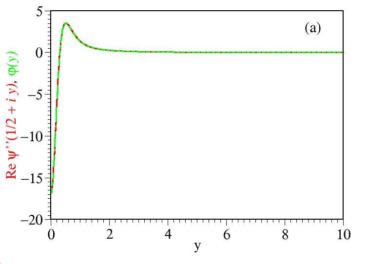
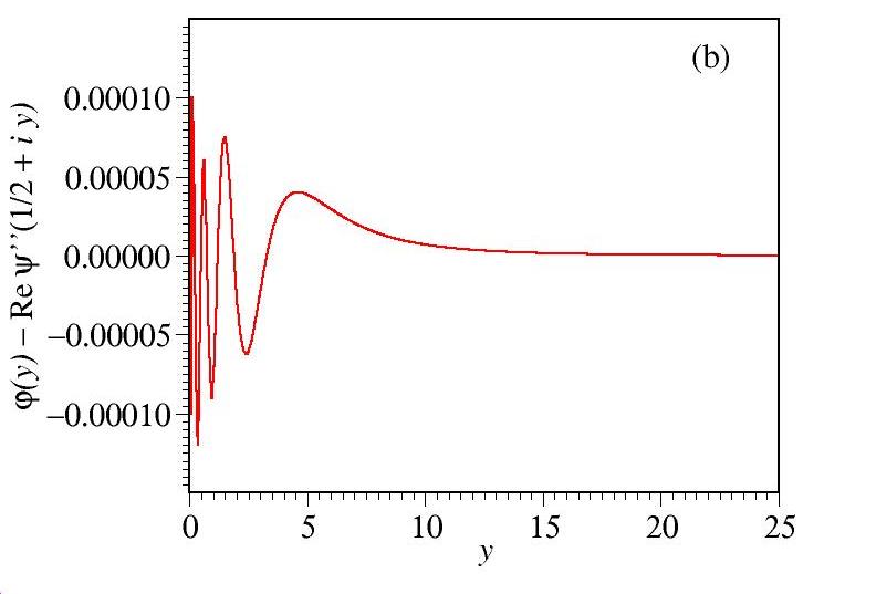
Figure 1: (a) The function $\varphi(y)$ expressed in terms of elementary functions (Equation (6b)) and the real part of the polygamma function $\mbox{Re}\,\psi(2;1/2+iy)$ depicted (b) along with their differences, revealing that Equation (6) is a very accurate approximation.

For parameter ranges covering virtually all experimental situations of interest wherein a $T$-dependent $G$ can be expected, the parameter

$$x\equiv\frac{\Gamma_{a}}{2\pi k_{B}T}$$ (6c)

is small, and the lowest order expansion of the RHS of Equation (4)

$$\displaystyle\frac{G}{G_{0}} \simeq \frac{\pi\Gamma_{g}^{2}}{4\Gamma_{a}k_{B}T}\mbox{sech}^{2}\pi y+\frac{\Gamma_{g}^{2}\varphi(y)}{\left(2\pi k_{B}T\right)^{2}}$$ (6d)

$$y \equiv \frac{\varepsilon_{0}}{2\pi k_{B}T}$$ (6e)

is a very accurate approximation of the exact Equation (4); it holds $\mathcal{O}\left(x^{2}\right)$, which amounts to an relative error of $\sim$1% for $\Gamma_{a}$ smaller than about $k_{B}T/2$. Notice the numerical factor 4 in the denominator of the first term of Equation (6d), which corrects the incorrect factor 16 (a typo) in Equation (6) of ref. Bâldea (2022). If (highly unlikely in real junctions exhibiting $T$-dependent transport) $x$ is not very small with respect to unity, the last term in the RHS of Equation (5) can also be included

$$\displaystyle\frac{G}{G_{0}} \simeq \frac{\pi\Gamma_{g}^{2}}{4\Gamma_{a}k_{B}T}\mbox{sech}^{2}\pi y+\frac{\Gamma_{g}^{2}\varphi(y)}{\left(2\pi k_{B}T\right)^{2}}$$ (6f)

$$+\frac{\pi}{16}\frac{\Gamma_{g}^{2}\Gamma_{a}}{\left(k_{B}T\right)^{3}}\left[2-\cosh(2\pi y)\right]\mbox{sech}^{4}(\pi y);$$

it holds $\mathcal{O}\left(x^{3}\right)$, which amounts to an relative error of $\sim$1% for $\Gamma_{a}$ smaller than about $1.4\,k_{B}T$. At temperatures lower than the aforementioned ($1.4\,k_{B}T~{}\raisebox{-1.29167pt}{$\stackrel{{\scriptstyle<}}{{\sim}}$}~{}\Gamma_{a}$), thermal effects are negligible and the zero temperature limit (Equation (8)) applies. Figure 2 illustrates the accuracy of the approximate Equation (6d,f) for parameter values characterizing the real molecular junctions considered in Section 2.3. The curves computed via Equation (6d,f) cannot be distinguished within the drawing accuracy from those obtained via the exact Equation (4) in Sections 2.2 and 2.3. Therefore, they will not be shown there.

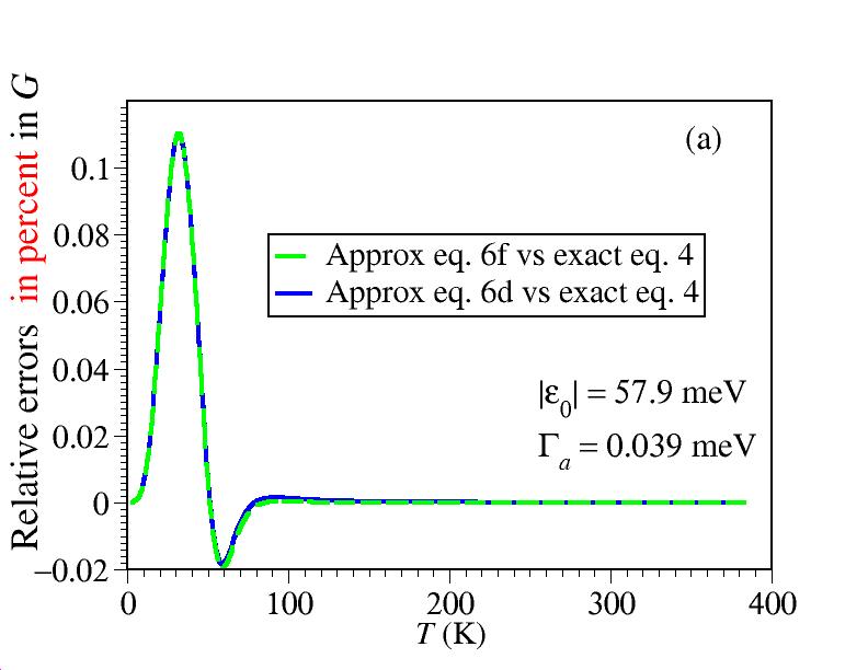
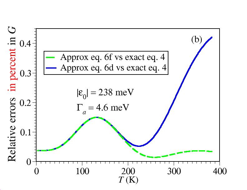
Figure 2: Relative errors in conductance $G$ for parameters (indicated in the legend) characterizing (a) the SET and (b) SAM setups (see below) illustrating that Equation (6d,f) represent very accurate approximation of the exact Equation (4).

Noteworthily, Equation (6d,f) only contain elementary functions. This is important for practical data fitting; special functions like trigamma entering Equation (4) are usually not implemented in common software packages used by experimentalists.

For parameter values where the peaks of the transmission function and the derivative of the Fermi function —possessing widths of the order $\Gamma_{a}$ and $k_{B}T$, and located at $\varepsilon=\varepsilon_{0}$ and $\varepsilon=0$, respectively—are sufficiently well separated in energy, the following approximate formula

$$\frac{G}{G_{0}}\simeq\underbrace{\frac{\pi}{4}\frac{\Gamma_{g}^{2}}{\Gamma_{a}k_{B}T}\mbox{sech}^{2}\frac{\varepsilon_{0}}{2k_{B}T}}_{G_{T}/G_{0}}+\underbrace{\frac{\Gamma_{g}^{2}}{\varepsilon_{0}^{2}+\Gamma_{a}^{2}}}_{G_{0K}/G_{0}}\xlongrightarrow{\Gamma_{a}\ll\left|\varepsilon_{0}\right|}\frac{\pi}{4}\frac{\Gamma_{g}^{2}}{\Gamma_{a}k_{B}T}\mbox{sech}^{2}\frac{\varepsilon_{0}}{2k_{B}T}+\frac{\Gamma_{g}^{2}}{\varepsilon_{0}^{2}}$$ (7)

generalizes a result deduced earlier Bâldea (2017) for $\Gamma_{s}=\Gamma_{t}=\Gamma_{a}=\Gamma_{g}$. It holds within $\sim$1% for $\Gamma_{a}$ smaller than about $k_{B}T/10$. Equation (7) reduces in turn to Equations (8) and (9) in the limit of very low and very high temperatures, generalizing results known from earlier studies Cuevas and Scheer (2017); Bâldea (2012); Sedghi et al. (2011); Garrigues et al. (2016); Smith et al. (2018).

$$\frac{G}{G_{0}}\xlongrightarrow{k_{B}T\ll\Gamma_{a}}\frac{G_{0K}}{G_{0}}=\frac{\Gamma_{g}^{2}}{\varepsilon_{0}^{2}+\Gamma_{a}^{2}}\xlongrightarrow{\Gamma_{a}\ll|\varepsilon_{0}|}\frac{\Gamma_{g}^{2}}{\varepsilon_{0}^{2}}$$ (8)

$$\frac{G}{G_{0}}\xlongrightarrow{\Gamma_{a}\ll\pi k_{B}T}\frac{G_{T}}{G_{0}}\equiv\frac{\pi}{4}\frac{\Gamma_{g}^{2}}{\Gamma_{a}k_{B}T}\mbox{sech}^{2}\frac{\varepsilon_{0}}{2k_{B}T}$$ (9a)

$$\frac{G}{G_{0}}\xlongrightarrow{\Gamma_{a}\ll\pi k_{B}T\ll\left|\varepsilon_{0}\right|}\frac{G_{p.A}}{G_{0}}=\frac{\pi\Gamma_{g}^{2}}{\Gamma_{a}k_{B}T}\exp\left(-\frac{\left|\varepsilon_{0}\right|}{k_{B}T}\right)$$ (9b)

(The above subscript $p.A$ stands for pseudo-Arrhenius).

Notice that unlike Equation (7), $T$ enters the RHS of Equation (6d,f) not only in the first term but also in the second term. Therefore, departures of Equation (7) from Equation (4) become substantial when $|\varepsilon_{0}|$, $\Gamma_{a}$, and $k_{B}T$ have comparable values. For this reason, for temperatures around $T_{c}$ (see Equation (11a) below), Equation (4) better quantifies the gradual transition between an Arrhenius-type (high $T$) and a Sommerfeld (low $T$) regime Bâldea (2022) than Equation (7).

Thermal corrections to Equation (8) can alternatively obtained via Sommerfeld expansion of Equation (1) and expressed in terms of the Riemann $\zeta$ function Sommerfeld and Bethe (1933); Jahnke and Emde (1945); Ashcroft and Mermin (1976)

$$\frac{G}{G_{0}}=\frac{1}{4}\sum_{n=0}^{\infty}\frac{\left(k_{B}T\right)^{2n}}{(2n)!}\left.\frac{\partial^{2n}}{\partial\varepsilon^{2n}}\mathcal{T}(\varepsilon)\right|_{\varepsilon=0}\int_{-\infty}^{\infty}x^{2n}\mbox{sech}^{2}\frac{x}{2}d\,x=\frac{G_{0K}}{G_{0}}+\sum_{n=1}^{\infty}\left(k_{B}T\right)^{2n}\left(2-\frac{1}{2^{2(n-1)}}\right)\zeta(2n)$$

which gives the first Sommerfeld correction (S1, $$\mathcal{O}\left(T^{2}\right)$$)

$$\frac{G}{G_{0}}\simeq\frac{\Gamma_{g}^{2}}{\varepsilon_{0}^{2}+\Gamma_{a}^{2}}\left[1+\left(\pi k_{B}T\right)^{2}\frac{\varepsilon_{0}^{2}-\Gamma_{a}^{2}/3}{\left(\varepsilon_{0}^{2}+\Gamma_{a}^{2}\right)^{2}}\right]$$ (10a)

and the second Sommerfeld correction (S2, $$\mathcal{O}\left(T^{4}\right)$$)

$$\frac{G}{G_{0}}\simeq\frac{\Gamma_{g}^{2}}{\varepsilon_{0}^{2}+\Gamma_{a}^{2}}\left[1+\left(\pi k_{B}T\right)^{2}\frac{\varepsilon_{0}^{2}-\Gamma_{a}^{2}/3}{\left(\varepsilon_{0}^{2}+\Gamma_{a}^{2}\right)^{2}}+\left(\pi k_{B}T\right)^{4}\frac{7}{15}\frac{5\varepsilon_{0}^{4}-10\varepsilon_{0}^{2}\Gamma_{a}^{2}+\Gamma_{a}^{4}}{\left(\varepsilon_{0}^{2}+\Gamma_{a}^{2}\right)^{4}}\right]$$ (10b)

Interestingly, there is no linear correction in $T$ to $G$ in the above formulas.

To end this general theoretical part, and in order to avoid confusion regarding the applicability to real molecular junctions, we want to emphasize that none of the above results quantifying thermal effects on the charge transport via tunneling is limited to a specific experimental platform, be it SET, EGaIn (to be examined in Sections 2.3 and 2.4), CP-AFM (considered earlier Smith et al. (2018)) or any other.

What is important for the single level model underlying Equation (1) is that the charge transport is “one-dimensional”, i.e., proceeds along individual molecules; loosely speaking, that an electron (or hole) leaving the left electrode does not tunnel across the left half of a molecule A, then jumps on a neighboring molecule B, and finishes the trip to the right electrode after tunneling across the right half of molecule B.

Importantly, the theoretical single level model utilized does not necessarily rule out an intermolecular (A-B) interaction. In an elementary transport process, an electron tunneling across molecule A can interact with the adjacent molecule B. Provided that the charge transport does not induce electron exchange between adjacent molecules A and B, the effects of this potentially significant intermolecular interaction translate into an extra level shift (i.e., renormalized $\varepsilon_{0}$) and an extra level broadening expressed as an additional term to the RHS of Equation (3)

$$\Gamma_{s}+\Gamma_{t}\to\Gamma_{s}+\Gamma_{t}+\Gamma_{env}$$

Above, the subscript “env” stands for environment. Because both $\varepsilon_{0}$ and $\Gamma_{a}$ are model parameters, the implications for data fitting are not dramatic.

The fact that in Section 2.4 we will be able to estimate the fraction $f$ of active molecules merely in terms of $\Gamma_{s}$ and $\Gamma_{t}$ (amounting to assume $\Gamma_{env}=0$) demonstrates that, at least for the large area EGaIn-based junctions considered there, intermolecular interaction effects do not have a dramatical impact on transport.

2.2 Results Illustrating the Temperature Impact on the Charge Transport by Tunneling

Insight into the thermal impact on the tunneling conductance can be gained by inspecting the results of numerical simulations depicted in Figures 3 and 4. Inspection of these figures reveals that, irrespective of the magnitude of the MO width $\Gamma_{a}$, up to $T\approx 340$ K—a value that safely covers the temperature range accessed in experiments Garrigues et al. (2016); Smith et al. (2018)—thermal effects are negligible for energy offsets $\left|\varepsilon_{0}\right|$ larger than about $0.4$ eV (cf. Figure 3d,e).

Below this value, thermal effects become significant. At a given level offset value $\left|\varepsilon_{0}\right|$, they are the more pronounced, the smaller the value of $\Gamma_{a}$ is (cf. Figure 3a–c). Likewise, at given level width $\Gamma_{a}$, thermal effects are the more pronounced, the smaller the level offset $\left|\varepsilon_{0}\right|$ is (cf. Figure 4a–c).

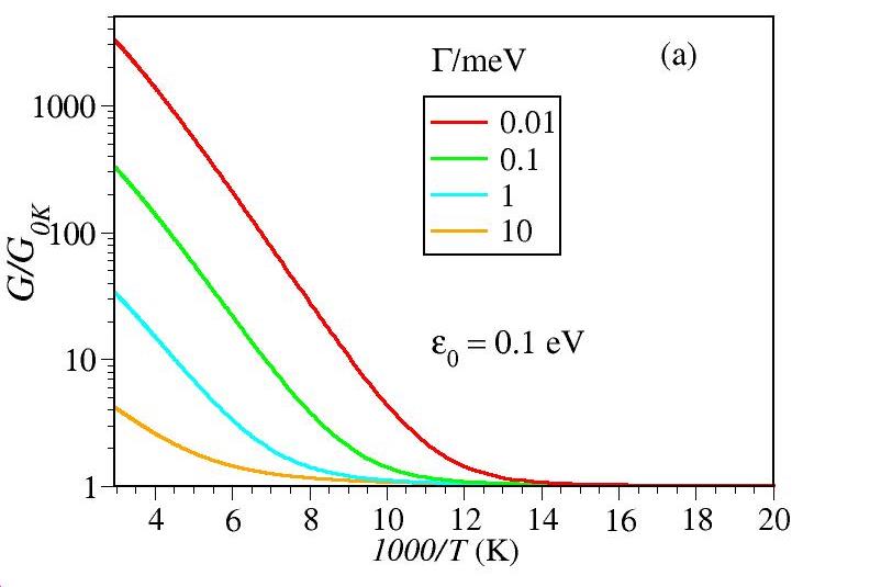
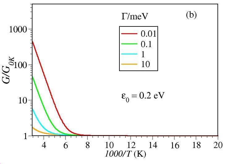
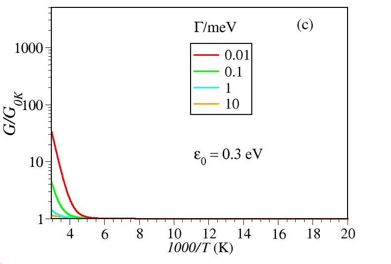
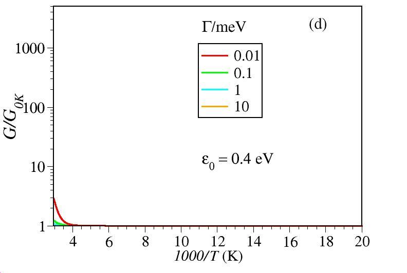
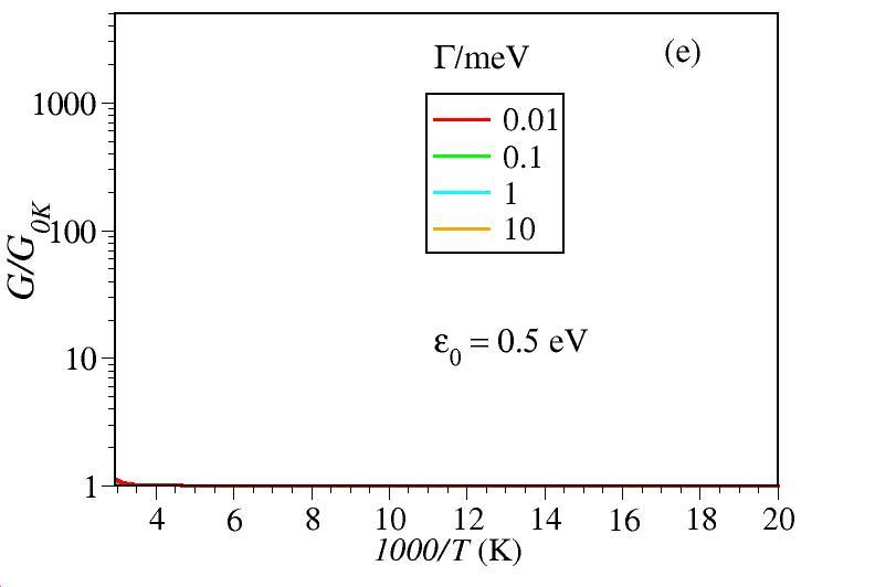
Figure 3: Simulating the temperature impact on the low bias conductance $G$ normalized to the zero temperature value $G_{0K}$. Impact of a variable level width $\Gamma_{a}$ at fixed energy offset $\varepsilon_{0}$. Notice that the range on the y-axis is the same all panels (a–e). At given $\varepsilon_{0}$, the impact of temperature is more pronounced at smaller $\Gamma_{a}$. As visible, thermal effects on $G$ are negligible for $\left|\varepsilon_{0}\right|$ larger than about 0.4 eV.

By and large, the message conveyed by Figures 3 and 4 is clear: temperature dependent measured data should by no means be taken as conclusive evidence for two-step hopping conduction (cf. ref. Bâldea (2022) and citations therein).

Figures 3 and 4 clearly illustrate that, for sufficiently (but realistically) small values of $\left|\varepsilon_{0}\right|$ and $\Gamma_{a}$ the single-step tunneling transport can exhibit a strong temperature dependence. At high $T$, the (pseudo-)Arrhenius behavior resulting from tunneling (cf. Equation (9b)) can hardly be distinguished from the traditional Arrhenius characteristic for charge transport via hopping. As the temperature is lowered, this Arrhenius-like regime $G\approx G_{T}$ (cf. Equation (9a)) gradually switches into a Sommerfeld regime Bâldea (2022), wherein thermal effects basically represent corrections (cf. Equation (10)) to the zero temperature value $G_{0K}$ (Equation (8)).

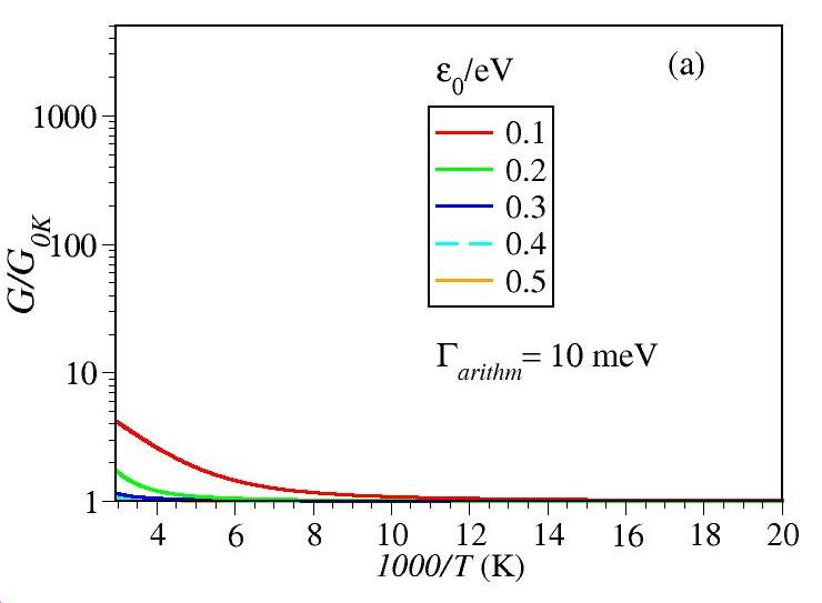
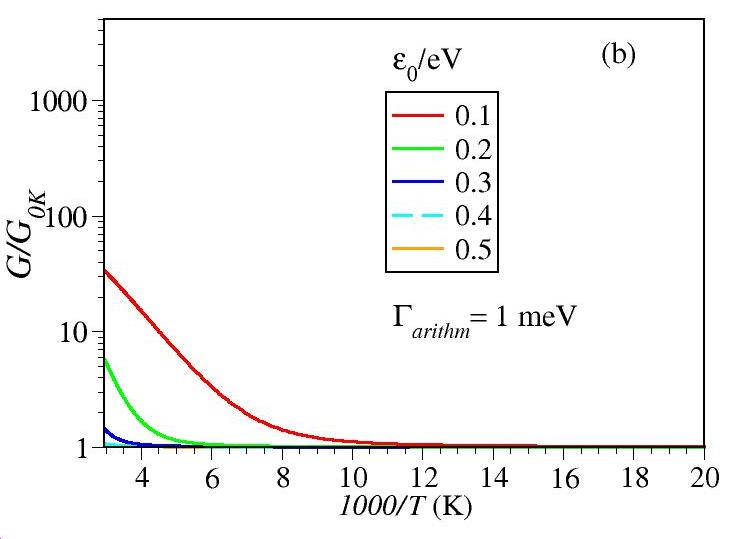
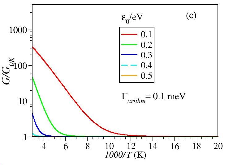
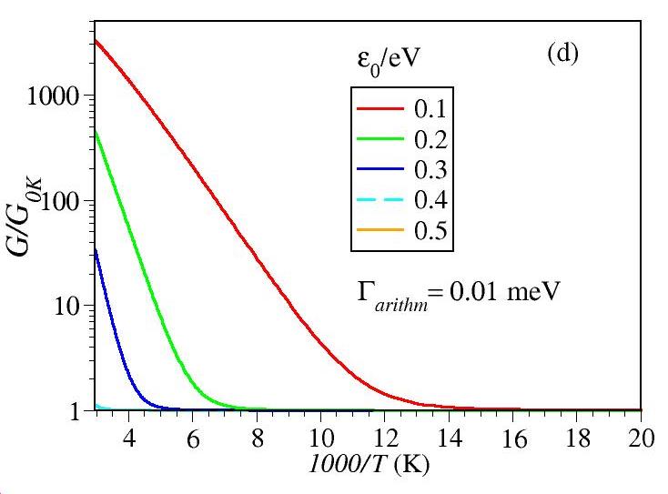
Figure 4: Simulating the temperature impact on the low bias conductance $G$ normalized to the zero temperature value $G_{0K}$. Impact of a variable level offset $\varepsilon_{0}$ at fixed $\Gamma_{a}$. At given $\Gamma_{a}$, the impact of temperature is more pronounced at smaller $\left|\varepsilon_{0}\right|$. Notice that the range on the y-axis is the same all panels (a–d).

Because this transition is gradual, a crossover (“critical” or “transition”) temperature $T_{c}$ separating these Arrhenius and Sommerfeld regimes can only be defined by some arbitrary convention. An intuitive possibility is to define $T_{c}$ by the point where extrapolated (dashed, nearly linear) curves of $G_{T}$ (Equation (9a)) cross the horizontal (dashed, cyan) line corresponding to the zero temperature value $G_{0K}$, Equation (11a) (Figure 5a). This “critical” temperature $T_{c}$ approximately corresponds to the temperature where the exact, temperature dependent value of $G$ represents twice the zero temperature value $G_{0K}$ (Equation (11b), magenta horizontal line in Figure 5a,d).

$$\left.G_{T}\right|_{T=Tc} = G_{0K}$$ (11a)

$$\left.G(T)\right|_{T=Tc} \approx 2G_{0K}$$ (11b)

Imposing Equation (11a) yields a curve of $T_{c}$ versus $\Gamma_{a}$ which is unique in the reduced quantities $T_{c}/\left|\varepsilon_{0}\right|$ and $\Gamma_{a}/\left|\varepsilon_{0}\right|$ (cf. Figure 5b). More specific illustrations are depicted in Figure 5c, which give a flavor on the values characterizing real molecular junctions. Noteworthily, the results presented in Figure 5 give additional support to a previous conclusion Bâldea (2017); contradicting a possible naive expectation, the crossover between a temperature dependent and temperature independent transport by tunneling occurs at a value of $k_{B}T_{c}$ which is, in general, substantially different from $\Gamma_{a}$.

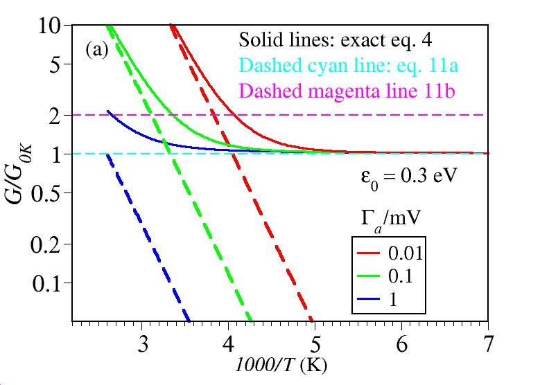
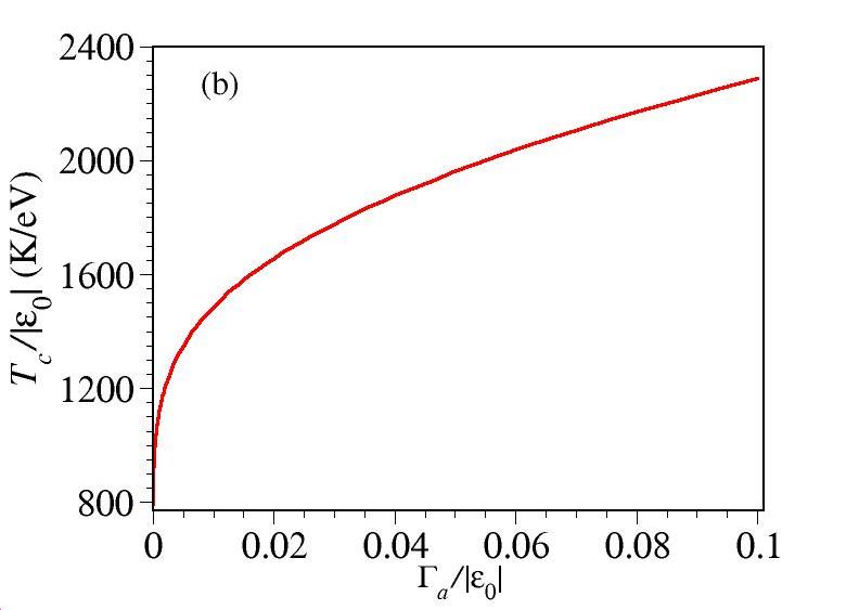
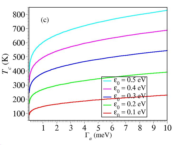
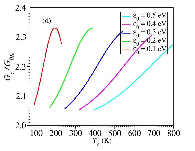
Figure 5: (a) In view of the gradual character of the Arrhenius-Sommerfeld transition, a “critical” (“transition”) temperature $T_{c}$ can only be defined by an arbitrary convention, e.g., where the inclined dashed lines depicting $G_{T}$ (Equation (9a)) cross the cyan horizontal line depicting the zero temperature conductance $G_{0K}$. Notice that at $T=T_{c}$ the exact conductance is, roughly, two times larger $G_{0K}$ (horizontal magenta line). (b) The curve of the critical temperature in dimensionless coordinates obtained using Equation (11a). (c) Curves for $T_{c}$ for various model parameter values indicated in the inset. (d) Curves showing that at $T=T_{c}$ the exact conductance $G_{c}=G\left(T_{c}\right)$ is approximately twice the zero temperature conductance $G_{0K}$.

2.3 Results for Specific Molecular Junctions

Out of the experimental results available for charge transport through molecular junctions at variable temperature Poot et al. (2006); Song et al. (2009); Heimbuch et al. (2012); McCreery et al. (2013); Asadi et al. (2013); Xiang et al. (2016); McCreery (2016); Garrigues et al. (2016); Kumar et al. (2016); Xin et al. (2017); Morteza Najarian and McCreery (2017); Smith et al. (2018); Xin et al. (2021), we will consider in this section the junctions fabricated with symmetric molecules consisting of a ferrocene unit (Fc) Haaland and Nilsson (1968); Coriani et al. (2006) contacted via alkyl spacers to electrodes Garrigues et al. (2016) in two testbeds. In single molecule transistor (SET) setup, -S-(CH2)4-Fc-(CH2)4-S- molecules were contacted to gold electrodes via thiol groups. In junctions based on self assembled monolayers (SAM), molecules were sandwiched between gold and EGaIn electrodes (Au-S-(CH2)6-Fc-(CH2)6-CH3/EGaIn).

We compared the theoretical zero bias conductance $G=G(T)$ with the quantity $j(T;V)/V$ estimated from the experimental currents $j(T;V)$ given in arbitrary units in ref. Garrigues et al. (2016) for the lowest bias $V$ (namely, at $V=10$ mV for SET for $80\,\mbox{K}\leq T\leq 220$ K and at $V=160$ mV for SAM for $220\,\mbox{K}\leq T\leq 330$ K).

To start with, we present in Figure 6 results obtained by fitting the experimental data (courtesy of C. A. Nijhuis and Y. Li) postulating an Arrhenius dependence

$$G=G_{\infty}\exp\left(-\frac{E_{a}}{k_{B}T}\right)$$ (12)

which corresponds to $\ln G$ varying linearly with inverse temperature $1/T$. The activation energies $E_{a}\simeq 45$ meV for SET and $E_{a}\simeq 160$ meV for SAM obtained using MATHEMATCA’s routine LinearModelFit shown in Figure 6 are similar to those from Figure 3 of ref. Garrigues et al. (2016).

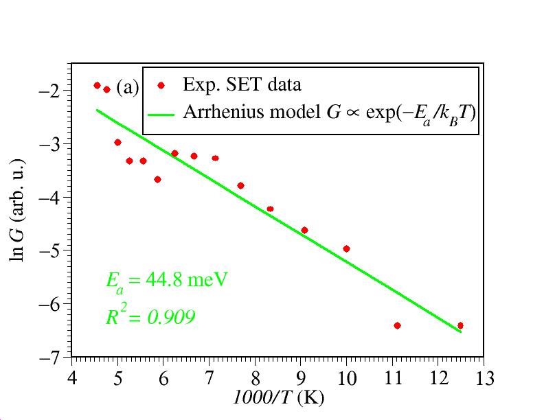
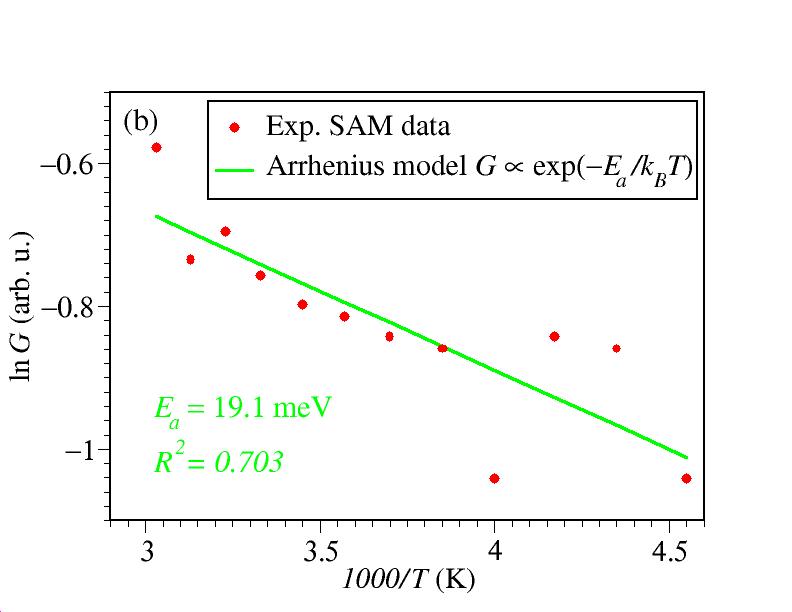
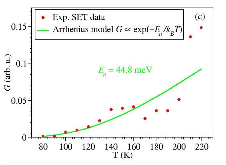
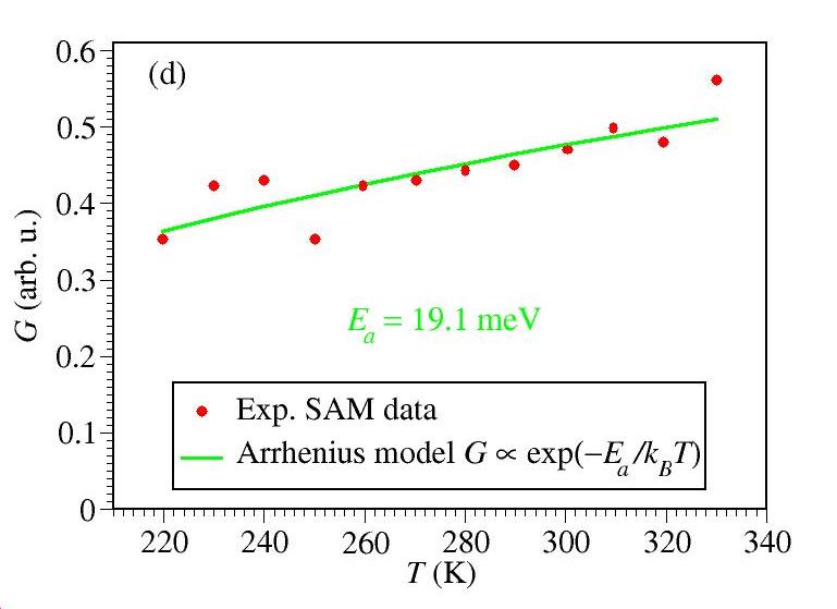
Figure 6: Arrhenius fits (Equation (12)) of the temperature dependent conductance $G$ of the ferrocene-based molecular junctions measured in ref. Garrigues et al. (2016) (courtesy of C. A. Nijhuis and Y. Li): (a) for SET setup at $V=10$ mV and (b) SAM setup at $V=160$ mV. They are recast in coordinates $G$ versus $T$ in (c,d), respectively. The values of $V$ indicated here correspond to the lowest bias results reported Garrigues et al. (2016).

However, as seen above, a pure Arrhenius dependence cannot be substantiated by the present model calculations. Model parameters estimated from data fitting using the various methods discussed in Section  2.1 are collected in Table 1. They show that even the pseudo-Arrhenius form $G\to G_{p.A}$ (Equation (9b)), which merely differs from $G_{A}$ by a prefactor $\propto 1/T$, yields significantly different “activation energies” ($\left|\varepsilon_{0}\right|\simeq 56$ meV for SET and $\left|\varepsilon_{0}\right|\simeq 44$ meV for SAM). We put “activation energies” in quotation marks because $\left|\varepsilon_{0}\right|$ does not represent a true barrier energy to be overcome by the charge carriers (in our specific case of HOMO-mediated conduction, holes Garrigues et al. (2016)).

Table 1: Parameter values estimated using various methods discussed in the main text. All quantities in meV.

Method	Property	SET	SAM
Equation (12)	$E_{a}$	45	19
Equation (9b)	$\left|\varepsilon_{0}\right|$	56	44
Equation (9a)	$\left|\varepsilon_{0}\right|$	57	53
Equation (7)	$\left|\varepsilon_{0}\right|$	58	193
	$\Gamma_{a}$	0.046	11
Equations (4), (6d) or (6f)	$\left|\varepsilon_{0}\right|$	58	238
	$\Gamma_{a}$	0.039	4.6

We recast the data depicted in Arrhenius coordinates ($\ln G$ versus $1/T$, Figure 6a,b) in coordinates $G$ versus $T$ (Figure 6c,d, respectively) to emphasize that, while not conspicuous for the case of SET, inferring an Arrhenius dependence from the measurements for the SAM-based junctions is highly problematic.

Figures 7a and 8a depict data fitting using the exact Equation (4) and MATHEMATICA’s routine NonlinearModelFit. Comparison between Figures 6d and 8a makes it clear why the MO energy offset estimated exactly for SAM ($\left|\varepsilon_{0}\right|\simeq 238$ meV) differs by an order of magnitude from the Arrhenius-based activation energy ($E_{a}\simeq 19$ meV). As visible (and also reflected in the different $R^{2}$-values), the fitting curve of Figure 6d better describes the general trend emerging the experimental data than the Arrhenius-based fitting curve of Figure 6d.

This difference is not so pronounced in the SET case (cf. Figures 6a and 7a). This explains why, although significant, the difference between the estimated MO energy offset ($\left|\varepsilon_{0}\right|\simeq 58$ meV) and the Arrhenius-based activation energy ($E_{a}\simeq 45$ meV) is not so dramatically large.

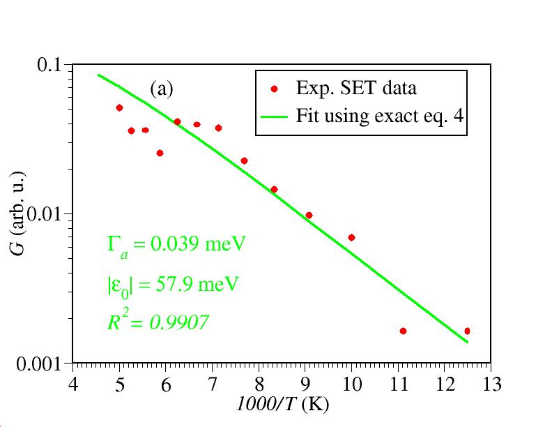
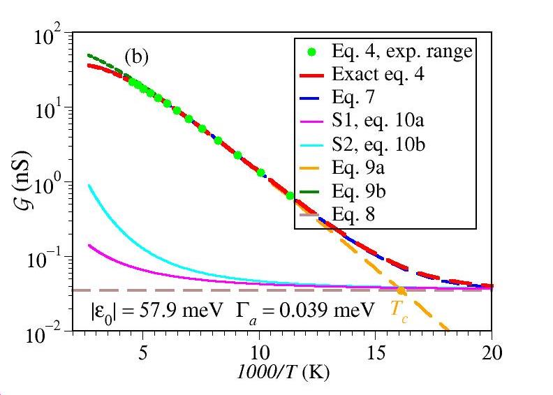
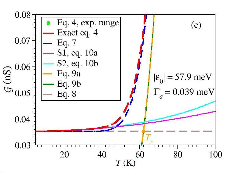
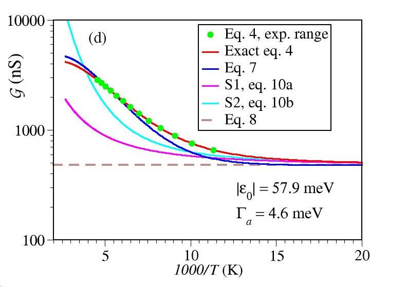
Figure 7: Results for SET setup. (a) Conductance ($G$) data at the lowest bias ($V=10$ mV) reported in ref. Garrigues et al. (2016) fitted using the exact Equation (4). (b) Exact curve $\mathcal{G}$ versus $1/T$ extrapolated beyond the temperature range sampled experimentally Garrigues et al. (2016) along with various approximations indicated in the legend. (c) Same as (b) recast as a function of $T$. (d) Same as (b) using the width value $\Gamma_{a}$ estimated for the SAM setup. For the meaning of $\mathcal{G}\propto G$, see Equation (13a) in the main text.

For comparison purposes, along with the exact curves for conductance, in Figures 7b,c and 8b,c we also show curves computed with the same parameters using various approximate formulas presented in Section 2.1. They are depicted for temperature ranges beyond those (indicated by green points) sampled in experiment, in order to emphasize that the experiments of ref. Garrigues et al. (2016) did not sample the Arrhenius-Sommerfeld transition for SET but partially sampled it for SAM.

Figure 7b reveals why for SET experiments Equation (7) represents a much more reasonable approximation than for SAM experiments (Figure 8c). In the former case, the temperatures explored experimentally are well below $T_{c}$ (the value of which is marked by an orange point), while in the latter case they are above $T_{c}$. The small asymptotic (zero temperature) value $G_{0K}$ depicted by the brown dashed line in Figure 7b makes it clear why Equation (9a,b) still reasonably describe the SET experimental data; Equation (9a) reasonably approximates Equation (7) in cases where $G_{0K}$ is small. Again, this is in contrast to the SAM data (Figure 8b,c).

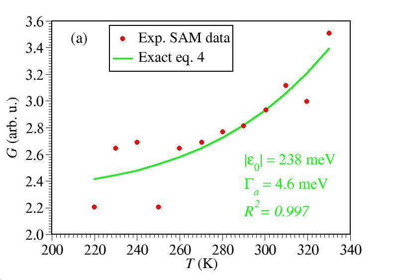
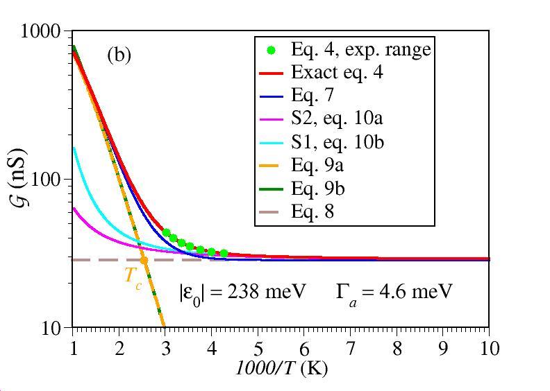
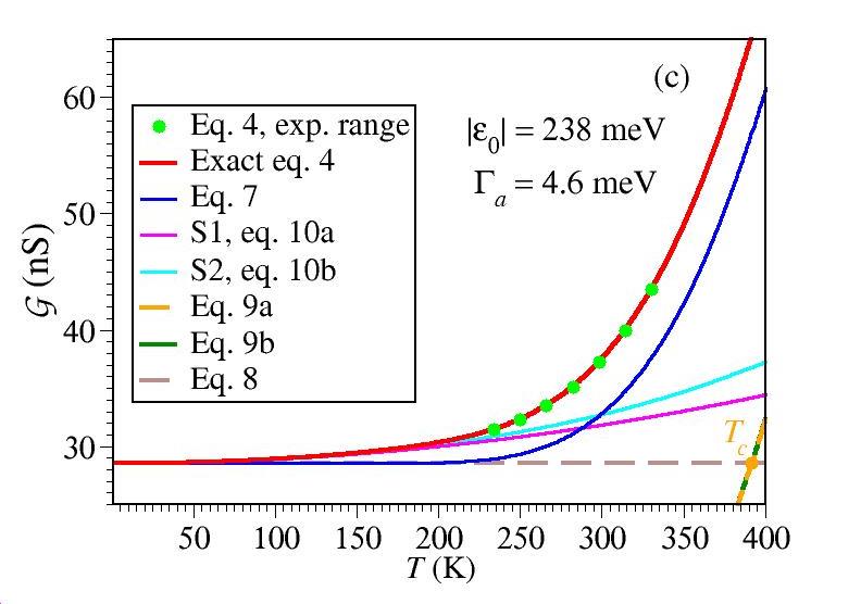
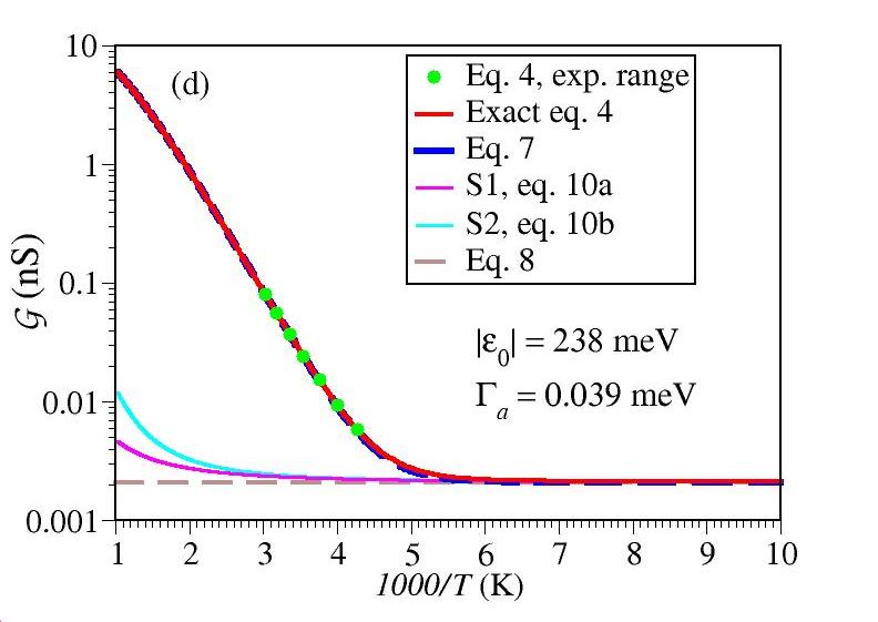
Figure 8: Results for SAM setup. (a) Conductance data at the lowest bias ($V=160$ mV) reported in ref. Garrigues et al. (2016) fitted using the exact Equation (4). (b) Exact curve $\mathcal{G}$ versus $1/T$ extrapolated beyond the temperature range sampled experimentally Garrigues et al. (2016) along with various approximations indicated in the legend. (c) Same as (b) recast as a function of $T$. (d) Same as (b) using the width value $\Gamma_{a}$ estimated for the SET setup. For the meaning of $\mathcal{G}\propto G$, see Equation (13a) in the main text.

Although the temperatures explored experimentally are above $T_{c}$, thermal effects exhibited by the SAM data do not merely represent corrections to the zero temperature limit. The SAM data do not simply belong to the pure Sommerfeld regime; the magenta (Equation (10a)) and cyan (Equation (10b)) curves in Figure 8b,c do significantly differ from the exact red curve (Equation (4)). In accord to those elaborated in Section 2.1, one could also note here that Figure 8b,c illustrate limitations of the interpolation expressed by Equation (7) in describing the crossover Arrhenius-Sommerfeld regime.

Let us briefly comment on the difference between the parameters for the SET and SAM. The relatively small difference between the values of $\varepsilon_{0}$ extracted form the SET and SAM data (58 meV versus 238 meV, respectively) can reflect effects due to the gate voltage ($V_{g}=-1.5$ V versus $V_{g}=0$) Song et al. (2009, 2011) and image charges (absent in the former case, present in the latter) Bâldea (2013). More importantly than differences in $\varepsilon_{0}$, $\Gamma_{a}$’s differ by two orders of magnitude. We assign this difference as an effect of the SAM-driven work function modification $\delta\Phi$. The strong (exponential) dependence of the molecule-electrode couplings on $\delta\Phi$ was amply documented in earlier studies Kim et al. (2011); Xie et al. (2015); Smith et al. (2018); Xie et al. (2019a, b).

To emphasize the important role played by $\Gamma_{a}$ in the Arrhenius-Sommerfeld transition, we also show curves for conductance computed for $\varepsilon_{0}$ determined for the SET setup and $\Gamma_{a}$ estimated for the SAM setup (Figure 7d) and vice versa (Figure 8d). In the former case, the temperature range sampled experimentally comprises the crossover region between the Arrhenius and Sommerfeld regimes. In the latter case, the temperature range sampled experimentally is shifted inside the Arrhenius regime.

2.4 The Arrhenius-Sommerfeld Thermal Transition: A Possible Approach to Estimate the Number of Molecules in Large Area Tunneling Molecular Junctions

In the various formulas presented above, $G$ is the conductance per molecule. Therefore, whatever the method utilized, fitting the transport measurements of ref. Garrigues et al. (2016) encounters an important difficulty: ref. Garrigues et al. (2016) only reported relative currents, not absolute currents. This is why, paradoxically, the discussion of this specific case is significantly more involved than the general methodology (Section 2.5) to be applied in cases where experimentalists report absolute (not relative) values of measured currents.

Fitting relative currents using Equation (9a,b) (as well as Equation (12), which was also used in ref. Garrigues et al. (2016)) merely allows the determination of $\left|\varepsilon_{0}\right|$. Data fitting using Equations (4), (6d,f) or (7) allows to obtain the values of $\left|\varepsilon_{0}\right|$ and $\Gamma_{a}$, but $\Gamma_{g}$ can only be obtained up to an unknown multiplicative factor.

For this reason, the value of $\Gamma_{g}$ was not indicated in Figures 7a and 8a, and $G$ was given in arbitrary units. What we showed in Figures 7b–d and 8b–d is the conductance per molecule $\mathcal{G}$ defined as

$$\mathcal{G}\equiv\left.G\right|_{\Gamma_{g}=\Gamma_{a}}$$ (13a)

which holds when the MO level is symmetrically coupled to electrodes (cf. Equations (2) and (3))

$$\Gamma_{a}=\Gamma_{g}\Leftrightarrow\Gamma_{s}=\Gamma_{t}$$ (13b)

To exemplify this, and for greater clarity, used in conjunction with Equation (4), $\mathcal{G}$ is expressed by

$$\frac{\mathcal{G}}{G_{0}}=\frac{\Gamma_{a}}{2\pi k_{B}T}\,\mbox{\small Re}\,\psi^{\prime}\left(\frac{1}{2}+\frac{\Gamma_{a}}{2\pi k_{B}T}+i\frac{\varepsilon_{0}}{2\pi k_{B}T}\right)$$ (13c)

The assumption in Equation (13b) is justified for the electrostatically gated SET (Au-S-(CH2)4-Fc-(CH2)4-S-Au) symmetrically adsorbed chemically via thiol groups, which are very likely single molecule devices Song et al. (2009); Bâldea and Köppel (2012). For this reason, $\mathcal{G}$ presented in Figure 7b is equal to the true (absolute, i.e., not relative) conductance value $G$. The absolute values calculated in this way appear to be consistent with the absolute values measured in experiment Garrigues et al. (2016), as far as they can be reconstituted after so many years del Barco .

Obviously, the above approach cannot be applied for the EGaIn large area SAM-based junctions having a nominal (geometric) area of $A_{\mbox{\small n}}\approx 700\,\upmu\mbox{m}^{2}$ Garrigues et al. (2016). The reason is twofold. First, they comprise an effective number of molecules $N_{\mbox{\small eff}}>1$. Above, we said “nominal area” and “effective number” because, as well documented Selzer et al. (2005); Milani et al. (2007); Akkerman and de Boer (2008); Simeone et al. (2013); Suchand Sangeeth et al. (2015); Sangeeth et al. (2016); Vilan et al. (2017); Mukhopadhyay et al. (2020), the effective (“electric”) area $A_{\mbox{\small eff}}$ may be on orders of magnitude smaller than $A_{\mbox{\small n}}$, or rephrased, because the total number of molecules $N_{n}$ in the junction is much larger than those effectively involved in charge transport:

$$f=\frac{A_{\mbox{\small eff}}}{A_{\mbox{\small n}}}=\frac{N_{\mbox{\small eff}}}{N_{\mbox{\small n}}}\ll 1$$ (14)

Second, the physical (van der Waals) EGaIn contact with the SAM is quantified by a coupling $\Gamma_{t}\equiv\Gamma_{t}^{\mbox{\small EGaIn}}$ substantially smaller than the chemical coupling $\Gamma_{s}\equiv\Gamma_{s}^{\mbox{\small Au}}$ to the gold substrate.

Put together, the following relations relating the presently calculated $\mathcal{G}$ and the conductance $G_{j}$ of the measured junction apply

$$G = \frac{\Gamma_{t}^{\mbox{\small EGaIn}}}{\Gamma_{s}^{\mbox{\small Au}}}\mathcal{G}$$ (15a)

$$N_{\mbox{\small eff}} = \frac{G_{j}}{G}=\frac{\Gamma_{s}^{\mbox{\small Au}}}{\Gamma_{t}^{\mbox{\small EGaIn}}}\frac{G_{j}}{\mathcal{G}}$$ (15b)

$$\Sigma = \frac{N_{\mbox{\small n}}}{A_{\mbox{\small n}}}=\frac{N_{\mbox{\small eff}}}{A_{\mbox{\small eff}}}$$ (15c)

$$\frac{N_{\mbox{\small eff}}}{N_{\mbox{\small n}}} = \frac{A_{\mbox{\small eff}}}{A_{\mbox{\small n}}}=\frac{\Gamma_{s}^{\mbox{\small Au}}}{\Gamma_{t}^{\mbox{\small EGaIn}}}\frac{G_{j}}{\mathcal{G}}\frac{1}{A_{\mbox{\small n}}\Sigma}$$ (15d)

Above, $\Sigma$ stands for the SAM coverage (number of molecules per unit area).

For SAMs of alkyl thiols and oligophenylene thiols utilized to fabricate CP-AFM junctions, measurements via Rutherford backscattering (RBS) and nuclear reaction analysis (NRA) provided coverage values $\Sigma\simeq 3.5$ molecules/nm² practically independent of the type of molecule Demissie et al. (2016); Xie et al. (2017).

Experiments have indicated similar coverage values of SAMs anchored via thiols on gold substrate used to fabricate CP-AFM junctions and EGaIn junctions Sangeeth et al. (2016). Therefore, the above value of $\Sigma$ is also reasonable for the presently considered SAM. For the EGaIn-based junctions of nominal contact area $A_{\mbox{\small n}}\approx 700\,\upmu\mbox{m}^{2}$ of ref. Garrigues et al. (2016), a nominal number of molecules per junction $N_{\mbox{\small n}}=A_{\mbox{\small n}}\Sigma\approx 2.45\times 10^{6}$ can thus be estimated.

At room temperature, we obtained the value $\mathcal{G}\simeq 37$ nS. As far as values measured more than eight years ago can be reconstitutedGarrigues et al. (2016), a junctions’s conductance $G_{j}\approx 20$ nS can be inferred Li . For CP-AFM junctions fabricated with alkyl thiols and gold substrate and tip electrodes, we recently estimated a ratio between the thiol chemisorbed contact and the methyl physisorbed contact of

$$\frac{\Gamma_{s}^{\mbox{\small Au}}}{\Gamma_{t}^{\mbox{\small Au}}}\simeq 37$$ (16)

If we used these values, we would deduce from Equation (15b) a value $N_{\mbox{\small eff}}\approx 20$, amounting to $f=N_{\mbox{\small eff}}/N_{\mbox{\small n}}=A_{\mbox{\small eff}}/A_{\mbox{\small n}}\approx 10^{-5}$. However, for the reason explained below, this value is underestimated.

Equation (16) assumed that both (substrate and tip/top) electrodes are of gold, which does not apply to the presently considered Au-(…Fc…)/EGaIn junctions. The EGaIn top electrode has a significantly different work function from gold. Using the dependence on the work function $\Phi$ of the effective coupling for CP-AFM junctions fabricated with alkyl monothiols (label $m$) and alkyl dithiols (label $d$) Xie et al. (2019b), we deduced

$$\Gamma_{m,d}\propto e^{\delta_{d,m}\,\Phi}$$ (17)

where $\delta_{m}=1.377\,\mbox{eV}^{-1}$ and $\delta_{d}=0.998\,\mbox{eV}^{-1}$. Following the method presented in ref. Bâldea (2021), we get

$$\Gamma_{t}\propto e^{\left(2\delta_{m}-\delta_{d}\right)\,\Phi}$$ (18)

and this yields

$$\frac{\Gamma_{t}^{\mbox{\small Au}}}{\Gamma_{t}^{\mbox{\small EGaIn}}}\approx\exp\left[\left(2\delta_{m}-\delta_{d}\right)\left(\Phi_{\mbox{\small Au}}-\Phi_{\mbox{\small EGaIn}}\right)\right]\approx 7$$ (19)

Above, we used the values $\Phi_{\mbox{\small EGaIn}}=4.1$ eV and $\Phi_{\mbox{\small Au}}=5.2$ eV. The fact that $G\propto\Gamma_{g}^{2}\propto\Gamma_{t}$ (cf. Equation (2)) translates into a corrected value

$$\frac{\Gamma_{s}^{\mbox{\small Au}}}{\Gamma_{t}^{\mbox{\small EGaIn}}}=\frac{\Gamma_{t}^{\mbox{\small Au}}}{\Gamma_{t}^{\mbox{\small EGaIn}}}\times\frac{\Gamma_{s}^{\mbox{\small Au}}}{\Gamma_{t}^{\mbox{\small Au}}}\approx 260$$ (20)

to be used instead of Equation (16) to compute $f$. With the above value, Equation (15b,c) yield $N_{\mbox{\small eff}}\approx 140$ and $A_{\mbox{\small eff}}\approx 40\,\mbox{nm}^{2}$. Indeed, these values are substantially smaller than $N_{\mbox{\small n}}\approx 2.45\times 10^{6}$ and $A_{\mbox{\small n}}\approx 700\,\upmu\mbox{m}^{2}$ indicated above. This amounts to

$$f=N_{\mbox{\small eff}}/N_{\mbox{\small n}}=A_{\mbox{\small eff}}/A_{\mbox{\small n}}\approx 0.6\times 10^{-4}$$ (21)

This fraction is comparable with area correction factors obtained using completely different methods reported earlier Yoon et al. (2014) for other EGaIn-based junctions. Possibly, this value is a general characteristics of the platforms using EGaIn top electrodes.

We have also to mention that oligophenyleneimines (OPI) junctions fabricated using EGaIn/Au electrodes were claimed Sangeeth et al. (2016) to be 100 times more resistive than OPI Au/Au CP-AFM junctions. The foregoing analysis found that Fc-based EGaIn junctions with alkyl thiol spacers are (only) seven times (cf. Equation (19)) more resistive than similar CP-AFM junctions. This suggests that care should be taken when comparing conducting properties of EGaIn and CP-AFM junctions fabricated with different molecular species, e.g., One should distinguish between localized electrons contributing to the dominant (HO)MO (read Fc-based junctions of ref. Garrigues et al. (2016)) and delocalized electrons (read OPI-based junctions of ref. Sangeeth et al. (2016)).

2.5 Workflow for Data Fitting

In the attempt to aid experimentalists in extracting information from low bias conductance measured at variable temperature, the workflow for the presently proposed data fitting is summarized in the diagram depicted in Figure 9. In addition, a few more details may be useful.

Experiments for large area junctions typically report current densities $j_{exp}\equiv j_{n}$, more precisely, current ($I$) values divided by the junction’s nominal area $A_{n}$. In the present low bias framework, the envisaged experimental quantity is the nominal conductance density $g_{exp}(T)\equiv g_{n}(T)$. Straightforward manipulation yields

$$g_{n}(T)\equiv\left.\frac{j_{n}(V;T)}{V}\right|_{V\approx 0}\equiv\left.\frac{1}{A_{n}}\frac{I(V;T)}{V}\right|_{V\approx 0}\equiv\frac{G_{j}(T)}{A_{n}}=\frac{A_{\mbox{\small eff}}}{A_{n}}\frac{N_{\mbox{\small eff}}}{A_{\mbox{\small eff}}}G(T)=\left(f\Sigma\right)G(T)$$ (22)

where $\Sigma$ is the SAM coverage. One should note that, whether data fitting is based on the exact Equation (4) or the various approximations based on it—namely, Equations (7), (6d) or (6f)—, the quantity $\Gamma_{g}^{2}$ always enters as a multiplicative factor the RHS of all those expression. Therefore, by stroke of Equation (22), one can use the combination

$$C\equiv f\Sigma\Gamma_{g}^{2}$$ (23)

as a unique fitting parameter. Data fitting based on any of the formulas mentioned above yields best fit estimates for $\varepsilon_{0}$, $\Gamma_{a}$, and $C$. The area correction factor $f$ can be estimated from $C$ and $\Gamma_{a}$ by stroke of Equations (2), (3) and (23) via the additional quantities $\Gamma_{s}$ and $\Gamma_{t}$, provided that an additional relationship between $\Gamma_{s}$ and $\Gamma_{t}$ exists.

For a specific illustration of how this relationship can be obtained for EGaIn-based large area junctions with alkyl spacers, see Equations (16)–(20). A similar strategy can be adopted in case of molecules of oligophenyls Xie et al. (2019a); Bâldea (2021) and oligoacenes Kim et al. (2011), for which the contact conductance data ($G_{C}\propto\Gamma_{g}^{2}=\Gamma_{s}\Gamma_{t}$) are also available.

The EGaIn-based junctions represent perhaps the most difficult case to handle. For other platforms (e.g., CP-AFM or crossed-wire Kushmerick et al. (2002a, b); Beebe et al. (2006)) using symmetric molecules symmetrically contacted to electrodes, the values of $\Gamma_{g}=\Gamma_{a}=\Gamma_{s}=\Gamma_{t}$ and $f$ can be straightforwardly be estimated from Equation (23). Obviously, provided that absolute values of the current (conductance) are available, there is no problem at all in the case single molecule junctions. There, $N_{\mbox{\small eff}}=N_{n}=1$, and $\Gamma_{g,a}$ and $\varepsilon_{0}$ can be directly obtained from data fitting.

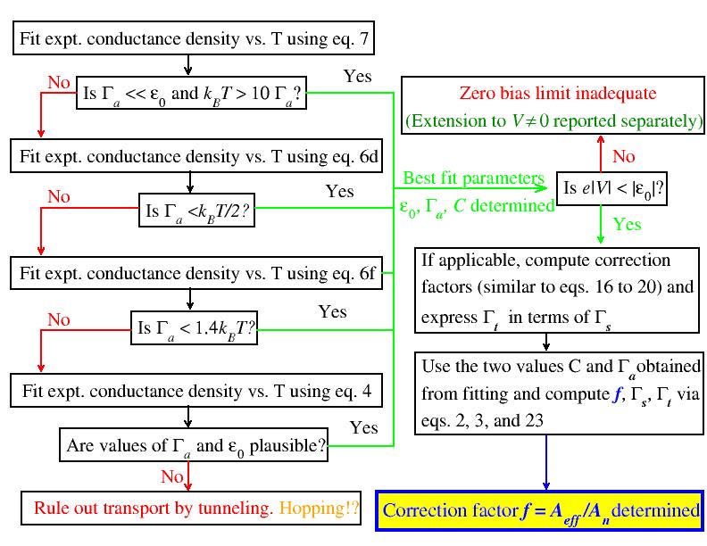
Figure 9: Diagram depicting the workflow for the presently proposed data fitting approach.

3 Method

The method utilized in ths paper is based on the general Keldysh formalism Caroli et al. (1971); Meir and Wingreen (1992); Haug and Jauho (2008); Cuevas and Scheer (2017) applied to the specified molecular junctions considered.

4 Conclusions

Routinely, a curve in “Arrhenius” plane ($\ln G$ versus $1/T$) which is a straight line is taken as evidence for charge transport via a two-step hopping mechanism, while a plot switching from a linear, inclined line to a horizontal line is taken as revealing a transition from two-step hopping to single-step tunneling conduction Choi et al. (2008); Hines et al. (2010), and a curve having a slope of magnitude progressively decreasing as $1/T$ increases is claimed to indicate a variable range hopping mechanism Shklovskii and Efros (1984).

The curves presented in this paper (e.g., Figures 3 and 4) demonstrate the drastic limitation of the oversimplified view delineated above. As we showed, all the aforementioned dependencies are fully compatible with a single-step coherent tunneling conduction. In a sufficiently broad temperature range, any curve $G$ versus $1/T$ computed by assuming a single-step tunneling mechanism switches from a roughly exponential shape (Arrhenius-like regime) at high $T$ to a less and less $T$-dependent Sommerfeld regime Bâldea (2022) at low $T$.

Whether only one of these regimes or both of them can be accessed in a real molecular junction depends, e.g., on the value of the crossover (“critical”) temperature $T_{c}$ (cf. Section 2.2 and Figure 5), on the temperature range that can be sampled experimentally, or on the thermal stability of the active molecule or electrodes. The latter are significant, e.g., for protein-based and EGaIn-based junctions, which can be employed in a rather restricted temperature range.

The Arrhenius-Sommerfeld transition can be more or less gradual. This is basically controlled by two parameters (level broadening $\Gamma_{a}$ and $\varepsilon_{0}$), which also set the value of $T_{c}$. Unlike $\varepsilon_{0}$ and $\Gamma_{a}$, $\Gamma_{g}$ essentially determines the magnitude of $G$; $T_{c}$ does not depend on $\Gamma_{g}$. In situations far apart from symmetry (e.g., $\Gamma_{s}\ll\Gamma_{t}\to\Gamma_{g}\ll\Gamma_{a}$), $\Gamma_{g}$ only indirectly affects the aforementioned interplay, in the sense that, if $G$ is too small at some temperatures, the corresponding $T$-range is experimentally irrelevant.

The various theoretical formulas, expressed in closed analytic forms, reported in this paper aims at assisting experimentalists in processing transport data measured at variable temperatures.

As an important application of those formulas, we used experimental data for ferrocene-based molecular junctions with an EGaIn top electrode to illustrate the possibility of estimating the number of molecules per junction, which is a property of paramount importance for large area junctions, wherein the effective (“electric”) area $A_{\mbox{\small eff}}$ can and does drastically differ from the nominal (“geometric”) area $A_{n}$. For the specific junctions considered, we obtained a value $A_{\mbox{\small eff}}/A_{n}\approx 0.6\times 10^{-4}$ compatible with other estimates for EGaIn-based junctions Yoon et al. (2014). To facilitate understanding practical details in implementing the presently proposed method of estimating the ratio $A_{\text{eff}}/A_{n}$, we showed a workflow diagram in Figure 9.

In this context, the advantage of the present formulas for $G=G(T)$—Equations (4), (6d,f) and (7)—as compared to other Arrhenius flavors (Equations (9a,b) and (12)) used previously in the literature becomes more evident. What the latter formulas can provide is merely an “activation energy” whose physical content is more or less obscure. In those formulas, $N\Gamma_{g}^{2}\to N_{\mbox{\small eff}}\Gamma_{g}^{2}$ enters as a unique fitting parameter. From the best fit estimate, $\Gamma_{g}$ can be computed only in situations where the effective number of molecules per junction $N_{\text{eff}}$ is known, but it is just this quantity that is the most problematic in case of large area junctions. For a similar reason, $N_{\text{eff}}/N_{n}$ cannot be confidently determined for cases where the experimentally accessed $T$-range merely lies in the nearly exponential fall-off (Arrhenius-like) part of the $G$-curve; the very weak dependence of $G$ on $\Gamma_{a}$ in such situations makes even the estimate for $\Gamma_{a}$ unreliable.

Fortunately, this was not an impediment in the case of SET Garrigues et al. (2016) examined in Section 2.3; although all measured data belong to the Arrhenius regime, the common value of $\Gamma_{a}\approx\Gamma_{g}$ can be estimated for symmetric, single-molecule platforms. With regard to the other (SAM-based) platform considered, the complete characterization of the SAM-based Fc junctions presented in Section 2.3 was possible just because the temperature range explore experimentally overlaps the Arrhenius-Sommerfeld crossover regime.

To end, we note that the determination of the number of molecules is an important issue not only for large area junctions but also, e.g., for CF-AFM junctions. Although models of contact mechanics Maugis (1992); Johnson (1985); Haugstad (2012) can be very useful to estimate the number of molecules in CP-AFM junctions Xie et al. (2017, 2019a, 2019b), reliable information needed (e.g., values of SAM’s Young moduli Bâldea (2021)) is often missing. The present method to estimate $N_{\mbox{\small eff}}$ can also applied for the CP-AFM platform.

Finally, we emphasize that the entire analysis elaborated in the present paper refers to the transport by tunneling; a coherent, single-step mechanism wherein (say,) electron (or hole) transfer from the left electrode to the (active) molecule is a process that cannot be separated from the electron transfer from the molecule to the right electrode. We did not consider the interplay between transport via tunneling and transport via hopping, which is a two-step mechanism wherein electron transfer from the left electrode to the molecule and electron transfer from the molecule to the right electrode are two distinct, uncorrelated processes characterized by durations much shorter than the electron’s residence time on the molecule, which is sufficiently long to allow molecular reorganization Bâldea (2013). A possible protocol to disentangle between tunneling and hopping conduction has been proposed Bâldea (2017) and applied Smith et al. (2018) elsewhere.

Financial support from the German Research Foundation (DFG Grant No. BA 1799/3-2) in the initial stage of this work and computational support by the state of Baden-Württemberg through bwHPC and the German Research Foundation through Grant No. INST 40/575-1 FUGG (bwUniCluster 2, bwForCluster/MLS&WISO 2/HELIX, and JUSTUS 2 cluster) are gratefully acknowledged.