Obtaining a Single-Photon Weak Value from Experiments using a Strong (Many-Photon) Coherent State

Abstract

A common type of weak-value experiment prepares a single particle in one state, weakly measures the occupation number of another state, and post-selects on finding the particle in a third state (a ‘click’). Most weak-value experiments have been done with photons, but the heralded preparation of a single photon is difficult and slow of rate. Here we show that the weak value mentioned above can be measured using strong (many-photon) coherent states, while still needing only a ‘click’ detector such as an avalanche photodiode. One simply subtracts the no-click weak value from the click weak-value, and scales the answer by a simple function of the click probability.

I Introduction: Coherence, Productivity, Post-Selection, and Jon

For the first and second authors, it is an alloyed pleasure to write a paper for this memorial volume celebrating Jonathan Dowling’s academic career. The passage of years gave us the distinction of being Jon’s long-time sparring partners, and then took that away. We beg the reader’s indulgence of our beginning the paper with some personal reminiscences, which also serve to say something about the topic of this paper. We will, eventually, motivate and present a new theory result at the intersection of quantum optics and quantum measurements, where Jon did much of his work. Moreover, the result is simple to state, and relatively simple to derive, but not immediately obvious, so we think Jon would have liked it.

We have all appreciated Jon’s iconoclasm. The first two authors (HMW and AMS) first encountered this during their PhDs, in Jon’s work on classical and quantum effects in cavity QED. For AMS, this was through hearing Jon talk in person, an aural experience still many years away for HMW. For HMW, it was, instead, through the publication of Jon’s delightfully titled paper on the topic, “Spontaneous emission in cavities: How much more classical can you get?”Dowling (1993). That paper demonstrated that an effect then widely celebrated as a dramatic consequence of quantum mechanics could in fact be observed in a strikingly classical setting as well. As shall be seen, this is also a theme of the present work, in an entirely different context. In the years since, both of us interacted with Jon many times, in many ways, some of which we will relate.

One way was that both HMW and AMS came to rely on Jon to do his utmost to help those of his colleagues more junior than himself. Another way relates to Jon’s famous redefinition of the Josephson Junction as the “time when a physicist must retire, go mad, or work to death,” which the editors of this volume rightly celebrate. Jon, of course, chose the last path, all too literally. On one occasion, he seemed to suggest that HMW had chosen another; see Fig. 1. (To be fair, he had further evidence, also implicating AMS; see Fig. 2.) It is certainly true that, unlike for HMW, Jon’s rate of production only increased following that occasion, while suffering no loss of coherence. These qualities — rate of production and coherence — provide another weak connection to the scientific topic of this paper: the measurement of a single-photon weak value using multi-photon coherent states, which comes with an enormous advantage in rate of production.

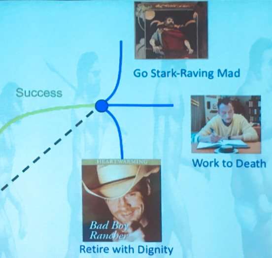
Figure 1: The Josephson Junction, as conceived by Jon Dowling. This is a photograph by the first author (HMW) of one of Jon’s slides at the Quantum Gates, Jumps, and Machines conference, Brisbane, October 2018. For the significance of the top picture, see https://howardwiseman.me/ThenArthurFought.html.

Figure 2: Further evidence provided by Jon in support of his case. Shockingly, said evidence was soon after removed by the editors of the (online only) journal in questionMahler et al. (2016).

A key component of weak values is post-selectionAharonov, Albert, and Vaidman (1988). Jon’s always creative vision made him an early adapter of photonic post-selection from linear-optics quantum computing to the task of preparing quantum states for quantum metrology or lithographyLee et al. (2002). This insight laid the groundwork for much of the work which the group of AMS went on to do on quantum metrology, and at one point led to Jon and AMS writing a grant proposal to pursue this further, along with Alex Lvovsky. No matter how hard AMS tried, he could not dissuade Jon from including a picture of a missile in the optical schematic (see Fig. 3). Perhaps the fact that, in the end, Jon was funded, but instructed to jettison AMS and Alex, says something about the perspicacity behind his seemingly insouciant iconoclasm.

The present work applies similar ideas of post-selection, but in this case in order to draw conclusions about what single photons would have done from experiments performed using coherent states and avalanche photodiodes. One can only smile to imagine the pleasure Jon would have taken in mocking us for doing this, after having pretended to take offense at AMS’s claim that a paper he was quite proud ofDeng et al. (2019) could have been done “with a light bulb”; see Fig. 4.

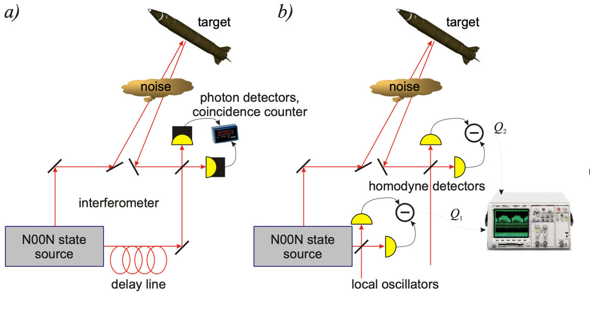
Figure 3: (a) Quantum imaging enables one to detect the perspicacity (target) behind Jon’s seemingly insouciant iconoclasm (noise). (b) With post-selection.

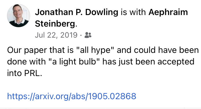
Figure 4: In another missile, Jon unfortunately misattributesOna to AMS the claim that his PRL was “all hype”. (AMS probably did say it could have been done with a light bulb.)

There are many reasons one might wish to study the evolution of individual quantum particles through the course of a process, for instance to ask how much we can say about “where a photon has been” as it traverses an interferometerDanan et al. (2013), how much time a particle spends tunneling through a barrierRamos et al. (2020), or whether or not a photon has been absorbed and reëmitted before being transmitted through a cloud of atomsSinclair et al. (2022). Yet while there have been dramatic advances in our abilities to produce and manipulate individual photonsWolfgramm et al. (2008); Steinlechner et al. (2012); Senellart, Solomon, and White (2017), the achievable rates are still far lower than the repetition rates of standard lasers. It is therefore interesting to ask whether there are measurements one can do on coherent states which nevertheless reveal something about the behaviour of individual photons. It is well known that G.I. Taylor’s 1909 interference experimentTaylor (1909), using a very weak classical light source, was later interpreted as confirming that “a single photon interferes with itself.” The quantum optics community long turned its back on such experiments, demanding nonclassical sources [e.g., measurements that $g^{(2)}<1$] in order to make statements about what individual photons actually do. At the same time, many modern workers have fruitfully applied the idea that a sufficiently weak coherent state is essentially a superposition of the vacuum and the single-photon state, so that “post-selecting” on detection of a photon projects out only the latter term, and is hence guaranteed to produce exactly the same results as a true single-photon experiment (see for exampleRitchie, Story, and Hulet (1991); Pittman and Franson (2003); Pittman et al. (2003); Mir et al. (2007); Hosten and Kwiat (2008); Dixon et al. (2009); Lundeen et al. (2011)).

While investigating the nonlinear phase shift which could be written by a single photonFeizpour et al. (2015), we (AMS and co-workers) found that the achievable shifts in our first experiment (${\cal O}(10\mu{\rm rad})$) would be too small to measure practically with the heralded-resonant-photon rates we had at our disposal (${\cal O}(100{\rm Hz})$). On the other hand, it was straightforward to generate weak coherent states at much higher rates. While at first we planned to limit these states to $|\alpha|^{2}\ll 1$ so that only the vacuum and single-photon contributions were significant, we came to the realization that this restriction was unnecessary. We showed that even if the experiment is done with a relatively strong coherent state at the input, in the situation where a detector placed at the output fires with low probability (e.g. because of collection or detection inefficiency), a click at that detector should lead one to update one’s estimate of the average number of photons present in that trial by adding 1. Thus by subtracting the nonlinear phase shift observed when the detector did not fire from that observed when it did, we learned how large the single-photon phase shift was: although the experiment always had a “background” of 30-100 photons in the coherent state, each time the detector fired, there would be the additional effect of that one “extra” photon. This led us to ask how far such reasoning could be pushed. Could we talk sensibly about the effects, or the history, of “that photon which had been detected”? In particular, would an earlier proposal for “amplifying” single-photon nonlinearities via postselectionFeizpour, Xing, and Steinberg (2011) work for photons post-selected in this fashion from a coherent source? We (MH, AMS, and co-workers) went on to show that it couldHallaji et al. (2017), in that specific case.

In this paper, we (the current authors) give a much more general proof that coherent states and click detectors can be used to measure single-particle occupation-number weak values, for arbitrary passive linear optical evolution before and after the weak measurement. The method is to subtract the no-click weak value from the click weak-value, and to scale this result by a simple function of the click probability. Thus, the click probability need not be kept small, and still no calibration of the coherent intensity or detector efficiency is necessary. We begin in Sec. II with notation and preliminaries, then the description of the experiment using coherent states in Sec. III. We give the main theorem, with proof, in Sec. IV, before concluding with Sec. V.

II Weak Values: Notation and Preliminaries

Consider the measurement of an observable $\Lambda$, represented by the Hermitian operator $\hat{\Lambda}$, using a weak coupling to a probe at time $t_{\rm p}$. Let the coupling be minimally disturbing (in the sense defined in Ref.Wiseman and Milburn (2010)) and let the initial probe state be such that the variable that will carry the information about $\Lambda$ has Gaussian statistics. Say the system is prepared in state $|{\psi_{\rm i}}\rangle$ at time $t_{\rm i}<t_{\rm p}$ and is found by a projective measurement at time $t_{\rm f}>t_{\rm p}$ to be in state $|{\phi_{\rm f}}\rangle$. Denote the expectation value, over very many runs of an experiment, post-selected on the final measurement result, of the weak measurement result, as ${}_{\langle{\phi_{\rm f}(t_{\rm f})}|}\langle{\Lambda}^{\rm w}_{t_{\rm p}}\rangle_{|{\psi_{\rm i}(t_{\rm i})}\rangle}$. Let the system evolve unitarily apart from the measurements, as described by the unitary operator $\hat{U}(t^{\prime},t)$ for evolution from $t$ to $t^{\prime}$. Then, as shown by Aharonov, Albert, and VaidmanAharonov, Albert, and Vaidman (1988); Aharonov and Vaidman (1990), quantum mechanics predicts that, in the limit of arbitrarily weak coupling, this so-called weak value is arbitrarily well approximated by

$${}_{\langle{\phi_{\rm f}(t_{\rm f})}|}\langle{\Lambda}^{\rm w}_{t_{\rm p}}\rangle_{|{\psi_{\rm i}(t_{\rm i})}\rangle}=\frac{\langle{\phi_{\rm f}}|\,\hat{U}(t_{\rm f},t_{\rm p})\hat{\Lambda}\,\hat{U}(t_{\rm p},t_{\rm i})|{\psi_{\rm i}}\rangle}{\langle{\phi_{\rm f}}|\,\hat{U}(t_{\rm f},t_{\rm i})|{\psi_{\rm i}}\rangle},$$ (1)

provided the denominator is nonzero. Actually, as described above, the weak value will be the real part of Eq. (1). However, the imaginary part can also be found experimentally by measuring the property of the probe conjugate to that which carries the information about $\Lambda$. See a particularly careful recent experimentVaidman et al. (2017).

Although this pure-state weak value has some unique featuresAharonov and Vaidman (1990); Vaidman et al. (2017), it is useful to generalise this resultWiseman (2002), and notation, to allow for an arbitrary final (post-selection) measurement, described by a positive operator $\hat{E}_{\rm f}$:

$${}_{{E_{\rm f}(t_{\rm f})}}\langle{\Lambda}^{\rm w}_{t_{\rm p}}\rangle_{|{\psi_{\rm i}(t_{\rm i})}\rangle}=\frac{\langle{\psi_{\rm i}}|\,\hat{U}(t_{\rm f},t_{\rm i})^{\dagger}\hat{E}_{\rm f}\,\hat{U}(t_{\rm f},t_{\rm p})\hat{\Lambda}\,\hat{U}(t_{\rm p},t_{\rm i})|{\psi_{\rm i}}\rangle}{\langle{\psi_{\rm i}}|\,\hat{U}(t_{\rm f},t_{\rm i})^{\dagger}\hat{E}_{\rm f}\,\hat{U}(t_{\rm f},t_{\rm i})|{\psi_{\rm i}}\rangle},$$ (2)

In this regard, the following Lemma will be used later.

Lemma 1

Consider a bipartite ($A\otimes B$) system and let $\hat{U}(t^{\prime},t)$ and $|{\psi_{\rm i}}\rangle$ be such that

$$\hat{U}(t_{\rm f},t_{\rm i})|{\psi_{\rm i}}\rangle=|{\psi^{A}_{\rm f}}\rangle\otimes|{\psi^{B}_{\rm f}}\rangle,$$ (3)

and consider $\hat{E}_{\rm f}=\hat{E}^{A}_{\rm f}\otimes\hat{I}$. Then

$${}_{{\left[{E}^{A}_{\rm f}\otimes{I}\right](t_{\rm f})}}\langle{\Lambda}^{\rm w}_{t_{\rm p}}\rangle_{|{\psi_{\rm i}(t_{\rm i})}\rangle}={}_{{\left[E^{A}_{\rm f}\otimes|{\psi^{B}_{\rm f}}\rangle\langle{\psi^{B}_{\rm f}}|\right](t_{\rm f})}}\langle{\Lambda}^{\rm w}_{t_{\rm p}}\rangle_{|{\psi_{\rm i}(t_{\rm i})}\rangle}.$$ (4)

That is, the same weak value is obtained whether one post-selects the second subsystem to be in state $|{\psi^{B}_{\rm f}(t_{\rm f})}\rangle$ or one simply ignores it.

Proof. Substituting both cases into Eq. (2) gives the same expression,

$$\frac{\left(\langle{\psi^{A}_{\rm f}}|\hat{E}_{\rm f}^{A}\otimes\langle{\psi^{B}_{\rm f}}|\right)\,\hat{U}(t_{\rm f},t_{\rm p})\hat{\Lambda}\,\hat{U}(t_{\rm p},t_{\rm i})|{\psi_{\rm i}}\rangle}{\langle{\psi^{A}_{\rm f}}|\hat{E}_{\rm f}^{A}|{\psi^{A}_{\rm f}}\rangle}.$$ (5)

$\square$

III Weak Values with Coherent States

Consider a multipartite system in which each subsystem is a photonic mode. We will use the Greek letters $\alpha$, $\beta$, and $\gamma$ to denote coherent states. More specifically, we will use upper-case Greek letters (${\rm A},{\rm B},\Gamma$) for the full multimode system, lower-case Greek letters for one particular mode (the first), and lower-case Greek letters with an over-arrow for all the modes but the first. Thus, for example,

$$|{\Gamma}\rangle\equiv|{\gamma,\vec{\gamma}}\rangle\equiv|{\gamma}\rangle|{\vec{\gamma}}\rangle\equiv|{\gamma}\rangle|{\gamma_{1}}\rangle|{\gamma_{2}}\rangle\cdots$$ (6)

Say that $\hat{U}(t^{\prime},t)$ is a passive linear optical transformation. That is, it takes a multimode coherent state to a multimode coherent state with the same mean photon number, $|\gamma|^{2}+|\vec{\gamma}|^{2}$. Let the system begin in a coherent state $|{\psi_{\rm i}}\rangle=|{{\rm A}}\rangle$, the weakly measured observable $\Lambda$ be the photon number $\hat{n}$ of some mode, and the post-selection be done by a photon number measurement on some final mode, yielding result $m\in\mathbb{N}_{0}$. Because $\hat{U}(t^{\prime},t)$ allows the modes to be defined in any way that is convenient, without loss of generality we can take

$$|{{\rm A}}\rangle=|{\alpha,\vec{0}}\rangle,\ \hat{\Lambda}=\hat{n}\otimes\hat{I}:=\hat{b}^{\dagger}\hat{b}\otimes\hat{I},\ \hat{E}_{\rm f}=|{m}\rangle\langle{m}|\otimes\hat{I}.$$ (7)

That is, the nominally first mode initially plays the role of the input pulse, then the weakly probed mode, then the mode on which the post-selection is made. This gives us the following short-hand notation:

$${}_{\langle{m}|}\langle{n}^{\rm w}_{t_{\rm p}}\rangle_{|{\alpha}\rangle}:={}_{{\left[|{m}\rangle\langle{m}|\otimes\hat{I}\right](t_{\rm f})}}\langle{[\hat{n}\otimes\hat{I}]}^{\rm w}_{t_{\rm p}}\rangle_{|{\alpha,\vec{0}\,(t_{\rm i})}\rangle}.$$ (8)

Figure 5: An example of the sort of situation under consideration, but with just two field modes in coherent states, i.e., $|{\alpha}\rangle|{\alpha_{1}}\rangle$, $|{\beta}\rangle|{\beta_{1}}\rangle$, and $|{\gamma}\rangle|{\gamma_{1}}\rangle$ at different stages in the evolution. Here the propagator $\hat{U}$ represents the evolution of the two modes through a Mach-Zehnder interferometer; a coherent state $|{\alpha}\rangle$ is incident from the left (at bottom), while vacuum is incident on the other port. We are interested in a weak measurement of the photon number in the bottom path (that is, the operator $\hat{b}^{\dagger}\hat{b}$), after post-selection upon a click at the detector in the upper port. The state entering that detector is, in the limit of arbitrarily weak measurement, arbitrarily well approximated by the coherent state $|{\gamma}\rangle$, where $|\gamma|^{2}=T|\alpha|^{2}$ as discussed in the text.

Let $\hat{U}(t_{\rm f},t_{\rm i})|{{\rm A}}\rangle=|{\Gamma}\rangle$. Then from Lemma 1, we have

$${}_{\langle{m}|}\langle{n}^{\rm w}_{t_{\rm p}}\rangle_{|{\alpha}\rangle}=\frac{\langle{m}|\langle{\vec{\gamma}}|\,\hat{U}(t_{\rm f},t_{\rm p})[\hat{b}^{\dagger}\hat{b}\otimes I]\,\hat{U}(t_{\rm p},t_{\rm i})|{\alpha,\vec{0}}\rangle}{\langle{m}|\langle{\vec{\gamma}}|\,\hat{U}(t_{\rm f},t_{\rm p})\,\hat{U}(t_{\rm p},t_{\rm i})|{\alpha,\vec{0}}\rangle},$$ (9)

Now for a given $\hat{U}(t_{\rm f},t_{\rm i})$, there exists a $T$ (transmittance) such that, for all $\alpha$,

$$|\gamma|^{2}=T|\alpha|^{2}.$$ (10)

Next, we consider the special case $m=0$. This case is indeed special because it is the only post-selection case where the final state is a coherent state. Specifically, defining

$$|{{\rm B}}\rangle=\,\hat{U}(t_{\rm p},t_{\rm i})|{\alpha,\vec{0}}\rangle,\ |{\tilde{\rm B}_{0}}\rangle=\,\hat{U}(t_{\rm p},t_{\rm f})|{0,\vec{\gamma}}\rangle,$$ (11)

it is easy to show from Eq. (9) that

$${}_{\langle{0}|}\langle{n}^{\rm w}_{t_{\rm p}}\rangle_{|{\alpha}\rangle}=\tilde{\beta}_{0}^{*}\beta\propto|\alpha|^{2},\ \langle{n}^{\rm w}_{t_{\rm p}}\rangle_{|{\alpha}\rangle}=|\beta|^{2}\propto|\alpha|^{2},$$ (12)

where the (non-appearing) proportionality constants would be fixed for $\hat{U}(t^{\prime},t)$ fixed. The second expectation value appearing in Eq. (12), the one without the left subscript, is the non-post-selected weak value. This of course coincides with the usual expectation value (for an arbitrary strength measurement) given the initial state.

Now, most experiments with photonic weak values have been done with avalanche photo-diodes, or some other detector that does not resolve photon-number. (See Ref.Chantasri et al. (2021) for a recent survey of weak value theory and experiments.) Such detectors can still be sensitive to single photons, but by only giving two results: no ‘click’, corresponding to $m=0$, and ‘click’, corresponding to all $m>0$, described by the positive operator $\hat{E}_{\star}:=\hat{I}-|{0}\rangle\langle{0}|$. For short, we just use ‘$\star$’ as the post-selecting subscript for a click, and from the operational definition of the weak value we have

$$\langle{n}^{\rm w}_{t_{\rm p}}\rangle_{|{\alpha}\rangle}=(1-p_{\star})\,{}_{\langle{0}|}\langle{n}^{\rm w}_{t_{\rm p}}\rangle_{|{\alpha}\rangle}\,+\,(p_{\star})\,{}_{{\star}}\langle{n}^{\rm w}_{t_{\rm p}}\rangle_{|{\alpha}\rangle},$$ (13)

where $p_{\star}=1-\exp(-T|\alpha|^{2})$ is the click probability. Equation (13) can also be derived from Eq. (2), noting that $\hat{I}=|{0}\rangle\langle{0}|+\hat{E}_{\star}$. One might worry that the calculation here would be insufficient for describing inefficient detectors. However, this is not the case. Detector inefficiency can always be modelled by a beam-splitter before a perfect detectorWiseman and Milburn (2010), and this is included in the allowed passive transformation $\hat{U}(t_{\rm f},t_{\rm i})$.

IV Weak Values with Single Photons, and the Theorem

Now, consider the case where the input is a single photon, $|{1}\rangle|{\vec{0}}\rangle$, rather than a coherent state, but with the weak measurement and post-selection as before. In this case a click unambiguously means a single photon, so we denote the weak values by ${}_{\langle{m}|}\langle{n}^{\rm w}_{t_{\rm p}}\rangle_{|{1}\rangle}$, where $m\in\{0,1\}$. Then, similar to Eq. (13),

$$\langle{n}^{\rm w}_{t_{\rm p}}\rangle_{|{1}\rangle}=(1-T){}_{\langle{0}|}\langle{n}^{\rm w}_{t_{\rm p}}\rangle_{|{1}\rangle}+T{}_{\langle{1}|}\langle{n}^{\rm w}_{t_{\rm p}}\rangle_{|{1}\rangle}.$$ (14)

This follows since $T$ is the probability of a successful post-selection (‘click’) in the single-photon case. This can be seen from Eq. (10) by considering the small $|\alpha|^{2}$ limit, to which we now turn.

There is a trivial and well-known (see in particular the Supplementary Information of Ref.Feizpour et al. (2015)) relation of this single-photon weak value to the coherent-state one, in the limit $|\alpha|^{2}\ll 1$. In this limit, the coherent-state input can be considered a superposition of vacuum, with probability amplitude close to unity, and a single photon, with probability amplitude $\alpha$. Moreover, any of the multimode coherent states considered above, such as $|{\Gamma}\rangle$, can be considered a superposition of vacuum and a single photon split across those modes with probability amplitudes for the latter equal to the components of $|{\Gamma}\rangle$. Thus it is simple to see that

$$\langle{n}^{\rm w}_{t_{\rm p}}\rangle_{|{\alpha}\rangle} =|\alpha|^{2}\langle{n}^{\rm w}_{t_{\rm p}}\rangle_{|{1}\rangle}+O(|\alpha|^{4}),$$ (15)

$${}_{{\star}}\langle{n}^{\rm w}_{t_{\rm p}}\rangle_{|{\alpha}\rangle} ={}_{\langle{1}|}\langle{n}^{\rm w}_{t_{\rm p}}\rangle_{|{1}\rangle}+O(|\alpha|^{2}).$$ (16)

The latter one follows because post-selecting on a click eliminates the vacuum component, and in the small $|\alpha|^{2}$ limit the single-photon term dominates.

In contrast with the above relations — which hold only in the limit of weak coherent states — here we derive a non-trivial relation between the weak values in the single-photon and coherent state cases, which holds for arbitrary coherent states, as follows.

Theorem 2

For any finite $|\alpha|^{2}>0$,

$${}_{\langle{1}|}\langle{n}^{\rm w}_{t_{\rm p}}\rangle_{|{1}\rangle}=\left[{}_{{\star}}\langle{n}^{\rm w}_{t_{\rm p}}\rangle_{|{\alpha}\rangle}-{}_{\langle{0}|}\langle{n}^{\rm w}_{t_{\rm p}}\rangle_{|{\alpha}\rangle}\right]f(p_{\star}),$$ (17)

where $f(x):=-x/{\ln(1-x)}$. That is, the single-photon weak-value can be found from an experiment using a coherent state of arbitrary size, and an avalanche photodiode, by subtracting the no-click weak value from the click weak-value, and multiplying by a function $f\in(0,1)$ of the click probability.

Proof. First, from the second proportionality in Eq. (12), it follows that there are in fact no higher-order terms in Eq. (15), and we can replace it by the exact expression

$$\langle{n}^{\rm w}_{t_{\rm p}}\rangle_{|{\alpha}\rangle}=|\alpha|^{2}\langle{n}^{\rm w}_{t_{\rm p}}\rangle_{|{1}\rangle}.$$ (18)

Second, we know from Eq. (12) that ${}_{\langle{0}|}\langle{n}^{\rm w}_{t_{\rm p}}\rangle_{|{\alpha}\rangle}=O(|\alpha|^{2})$ for small $|\alpha|^{2}$. Thus, expanding Eq. (13) in powers of $|\alpha|^{2}$ gives

$$\langle{n}^{\rm w}_{t_{\rm p}}\rangle_{|{\alpha}\rangle}={}_{\langle{0}|}\langle{n}^{\rm w}_{t_{\rm p}}\rangle_{|{\alpha}\rangle}\,+\,T|\alpha|^{2}\,{}_{{\star}}\langle{n}^{\rm w}_{t_{\rm p}}\rangle_{|{\alpha}\rangle}\,+\ O(|\alpha|^{4}).$$ (19)

Substituting into this Eqs. (16) and (18) yields

$${}_{\langle{0}|}\langle{n}^{\rm w}_{t_{\rm p}}\rangle_{|{\alpha}\rangle}=|\alpha|^{2}\left(\langle{n}^{\rm w}_{t_{\rm p}}\rangle_{|{1}\rangle}-T{}_{\langle{1}|}\langle{n}^{\rm w}_{t_{\rm p}}\rangle_{|{1}\rangle}\right)+O(|\alpha|^{4}).$$ (20)

Using Eq. (14), we obtain

$${}_{\langle{0}|}\langle{n}^{\rm w}_{t_{\rm p}}\rangle_{|{\alpha}\rangle}=|\alpha|^{2}(1-T){}_{\langle{0}|}\langle{n}^{\rm w}_{t_{\rm p}}\rangle_{|{1}\rangle}+O(|\alpha|^{4}).$$ (21)

But again using Eq. (12), it follows that the higher-order terms here are also zero, so we have another exact expression,

$${}_{\langle{0}|}\langle{n}^{\rm w}_{t_{\rm p}}\rangle_{|{\alpha}\rangle}=|\alpha|^{2}(1-T){}_{\langle{0}|}\langle{n}^{\rm w}_{t_{\rm p}}\rangle_{|{1}\rangle}.$$ (22)

Substituting Eqs. (18) and (22) into Eq. (14) yields

$${}_{\langle{1}|}\langle{n}^{\rm w}_{t_{\rm p}}\rangle_{|{1}\rangle}=\left({\langle{n}^{\rm w}_{t_{\rm p}}\rangle_{|{\alpha}\rangle}-{}_{\langle{0}|}\langle{n}^{\rm w}_{t_{\rm p}}\rangle_{|{\alpha}\rangle}}\right)/T|\alpha|^{2}.$$ (23)

Using (13) once more gives the desired result, (17). $\square$

Remark. It is no coincidence that the multiplicative factor $f(p_{\star})$ in Eq. (17) is simply the reciprocal of the average number of photons contributing to the click event ($m>0$). This average is $\bar{m}_{\star}\equiv\bar{m}/p_{\star}$, which evaluates to $T|\alpha|^{2}/\left[1-\exp(-T|\alpha|^{2})\right]$ for a Poisson distribution. In the limit of small $p_{\star}$, click events almost always involve only a single photon, and this factor goes to $1$. That is, in this limit, the single-photon weak value reduces to the difference between the click and no-click coherent weak values.

IV.1 Dark Accounting

As discussed already, detector inefficiency makes no difference to the above result. But there is another common detector imperfection: dark counts. Perhaps surprisingly, our result can very easily generalized to take this into account. Let $\check{p}$ be the probability of a dark count in the experiment if $\alpha=0$. For detectors with a finite dark-count rate, this would require defining a time-window for the experiment. Let us use $\check{0}$ and $\check{\star}$ to denote the events of a null-count and a non-null count in the situation where the non-null count could result from a dark count. Considering the probabilistic processes that can give rise to the two outcomes we are considering, we have

$$p_{\check{0}} =(1-p_{\star})(1-\check{p}),$$ (24)

$$p_{\check{\star}} =\check{p}+p_{\star}(1-\check{p}).$$ (25)

Then, from the operational definitions of weak values,

$${}_{{\check{0}}}\langle{n}^{\rm w}_{t_{\rm p}}\rangle_{|{\alpha}\rangle} ={}_{\langle{0}|}\langle{n}^{\rm w}_{t_{\rm p}}\rangle_{|{\alpha}\rangle},$$ (26)

$$p_{\check{\star}}\times{}_{{\check{\star}}}\langle{n}^{\rm w}_{t_{\rm p}}\rangle_{|{\alpha}\rangle} =p_{\star}\times{}_{{\star}}\langle{n}^{\rm w}_{t_{\rm p}}\rangle_{|{\alpha}\rangle}+(p_{\check{\star}}-p_{\star}){}_{\langle{0}|}\langle{n}^{\rm w}_{t_{\rm p}}\rangle_{|{\alpha}\rangle}.$$ (27)

Rearranging, we obtain

$$p_{\check{\star}}\left({{}_{{\check{\star}}}\langle{n}^{\rm w}_{t_{\rm p}}\rangle_{|{\alpha}\rangle}-{}_{{\check{0}}}\langle{n}^{\rm w}_{t_{\rm p}}\rangle_{|{\alpha}\rangle}}\right)=p_{\star}\left({{}_{{\star}}\langle{n}^{\rm w}_{t_{\rm p}}\rangle_{|{\alpha}\rangle}-{}_{\langle{0}|}\langle{n}^{\rm w}_{t_{\rm p}}\rangle_{|{\alpha}\rangle}}\right).$$ (28)

From this, we derive a simple generalization of Theorem 2:

Corollary 3

For any finite $|\alpha|^{2}>0$ and $\check{p}\geq 0$,

$${}_{\langle{1}|}\langle{n}^{\rm w}_{t_{\rm p}}\rangle_{|{1}\rangle}=\left[{}_{{\check{\star}}}\langle{n}^{\rm w}_{t_{\rm p}}\rangle_{|{\alpha}\rangle}-{}_{{\check{0}}}\langle{n}^{\rm w}_{t_{\rm p}}\rangle_{|{\alpha}\rangle}\right]g(\check{p},p_{\check{\star}}),$$ (29)

where (with $f$ as in Theorem 2),

$$g(y,z):=\frac{z(1-y)}{z-y}f\left({\frac{z-y}{1-y}}\right)$$ (30)

That is, the single-photon weak-value can be found from an experiment using a coherent state of arbitrary size, and an avalanche photodiode with dark counts, by subtracting the no-click weak value from the click weak-value, and multiplying by a function $g\in(0,\infty)$ of the dark ($|\alpha|^{2}=0$) click probability $\check{p}$ and the non-dark (actual $|\alpha|^{2}$) click probability $p_{\check{\star}}$.

V Discussion

We have shown that weak-valued properties of a single photon can be determined experimentally using a coherent state input in place of a single-photon input, and a simple click/no-click detector. Importantly, it is not necessary for the coherent state to be weak (i.e., have a mean photon number much less than one). This is of particular use in the case that the post-selection event in the single-photon case is rare, which is often the case for ‘interesting’ weak value experiments, where an anomalous value (in this case, outside the range $[0,1]$) is soughtRitchie, Story, and Hulet (1991); Pryde et al. (2005); Lundeen and Steinberg (2009); Dixon et al. (2009); Hallaji et al. (2017); Vaidman et al. (2017); Rebufello et al. (2021). Thus, when using a coherent state, the click probability $p_{\star}$ could be made much larger than the single-photon click probability $T$, giving a much higher data rate than even heralded single photons. In addition, coherent states can, of course, be produced on demand much more easily than single-photon states.

Another advantage of the coherent state option is that high-efficiency detectors are not needed. As discussed, detector inefficiency can always be modelled by a beam-splitter before the detection. From this it can be shown that a low-efficiency detector does not change the weak value in the single-photon case, but, because it reduces the click-probability $T$, it entails more runs being needed to obtain a large enough ensemble to give a weak value with the desired accuracy. In the coherent-state case, by contrast, the intensity $|\alpha|^{2}$ can simply be tuned to compensate for a low detection efficiency. Similar comments hold for optical losses in any part of the evolution, as long as the loss is the same along any path leading from the initial state to the detector.

As we have shown, a minor modification of our protocol also allows the effect of detector dark counts to be removed. If dark counts were a significant problem, then even for a single-photon experiment one would have to subtract the no-click weak value from the click weak value to obtain the desired result, enfeebling any objection to the coherent-state method on the basis of its indirectness. An even simpler generalization of our result would be to allow more than one mode to be coupled weakly to the probe at time $t_{\rm p}$, and to allow more than one mode to have its photon number measured at time $t_{\rm f}$. The proof is left as an exercise to the reader. On the other hand, it must be emphasized that our result holds only when the observable that couples to the probe in the experiment is the photon number of a mode (or set of modes, as just discussed). Without this, Eq. (12) would not hold and the theorem would not go through. It is easy to construct a counter-example by considering the operator $\hat{\Lambda}=\hat{I}\otimes\hat{I}$.

Given our peninitial paragraph, the reader may be wondering whether this penultimate paragraph will deliver the punch line “Single-photon weak values: How much more classical can you get?” Well, it just did, but in fact we argue the opposite. As mentioned above, the weak values we consider can be anomalous, such as when ${}_{\langle{1}|}\langle{n}^{\rm w}_{t_{\rm p}}\rangle_{|{1}\rangle}<0$. Moreover, PuseyPusey (2014) showed that any anomalous weak value is a proof of contextuality; such a thing cannot arise in a classical theory. Now, we have shown that ${}_{\langle{1}|}\langle{n}^{\rm w}_{t_{\rm p}}\rangle_{|{1}\rangle}$ can be obtained as the positively scaled difference of two differently post-selected averages of weak measurements of a positive operator ($\hat{n}$) with a coherent-state input, rather than as one such post-selected average with a single-photon input. Obviously a difference of two positive values can be negative, raising the possibility that in our scheme a classical explanation exists. However, our result includes as a special case the limit of a very weak input coherent state, in which case the subtracted value is negligible, meaning that the anomalous negativity of the weak value can arise from a single post-selected average with a coherent state. Therefore, despite the seeming classicality of coherent states and click detectors, there can be no classical explanation of the weak values in our general scenario. In this regard, one should remember that a non-destructive weak measurement of photon number is also an essential ingredient in the weak-value experiments we consider.

To conclude, our result motivates further directions for investigation. We have considered photon detection which does not resolve among different positive photon numbers. As Remarked upon above, in the limit of small $p_{\star}$, the single-photon weak value reduces to the difference between the click and no-click weak values. Moreover, for any value of $p_{\star}$, this difference is exactly equal to the single-photon weak value multiplied by the average number of photons involved in a “click” event. This supports earlier approximate results which suggested that if a photon-number resolving detector were used, the weak value post-selected on detecting $m$ photons would exceed the no-click weak value by precisely $m$ times the single-photon number. We leave a rigorous proof of this conjecture for future work.

Data Availability Statement

Data sharing is not applicable to this article as no new data were created or analyzed in this study

Conflict of interest

The authors have no conflicts to disclose.

REFERENCES

REFERENCES

- Dowling (1993) J. Dowling, “Spontaneous emission in cavities: How much more classical can you get?” Found. Phys. 23, 895–905 (1993).
- Mahler et al. (2016) D. H. Mahler, L. Rozema, K. Fisher, L. Vermeyden, K. J. Resch, H. M. Wiseman, and A. Steinberg, “Experimental nonlocal and surreal Bohmian trajectories,” Science Advances 2 (2016), 10.1126/sciadv.1501466.
- Aharonov, Albert, and Vaidman (1988) Y. Aharonov, D. Z. Albert, and L. Vaidman, “How the result of a measurement of a component of the spin of a spin-1/2 particle can turn out to be 100,” Physical Review Letters 60, 1351–1354 (1988).
- Lee et al. (2002) H. Lee, P. Kok, N. J. Cerf, and J. P. Dowling, “Linear optics and projective measurements alone suffice to create large-photon-number path entanglement,” Physical Review A 65, 030101 (2002).
- Deng et al. (2019) Y.-H. Deng, H. Wang, X. Ding, Z.-C. Duan, J. Qin, M.-C. Chen, Y. He, Y.-M. He, J.-P. Li, Y.-H. Li, et al., “Quantum interference between light sources separated by 150 million kilometers,” Physical Review Letters 123, 080401 (2019).
- (6) In loving memory of Jon’s refusal to ever let an editor have the last word, we were sorely tempted to accept our LaTeX editor’s suggestion to replace the apparently nonexistent word “misattributes” by (@hem) “m@sturb@tes”, perhaps confirming another of his affirmations: that in Fig. 2. We were also tempted to place that figure here, as Jon would certainly have appreciated a footnote to a figure caption containing a captured figure quoting a figurative footnote, which was in itself equally self-referential and silly.
- Danan et al. (2013) A. Danan, D. Farfurnik, S. Bar-Ad, and L. Vaidman, “Asking photons where they have been,” Physical Review Letters 111, 240402 (2013).
- Ramos et al. (2020) R. Ramos, D. Spierings, I. Racicot, and A. M. Steinberg, “Measurement of the time spent by a tunnelling atom within the barrier region,” Nature 583, 529–532 (2020).
- Sinclair et al. (2022) J. Sinclair, D. Angulo, K. Thompson, K. Bonsma-Fisher, A. Brodutch, and A. M. Steinberg, “Measuring the time atoms spend in the excited state due to a photon they do not absorb,” PRX Quantum 3, 010314 (2022).
- Wolfgramm et al. (2008) F. Wolfgramm, X. Xing, A. Cerè, A. Predojević, A. M. Steinberg, and M. W. Mitchell, “Bright filter-free source of indistinguishable photon pairs,” Opt. Express 16, 18145–18151 (2008).
- Steinlechner et al. (2012) F. Steinlechner, P. Trojek, M. Jofre, H. Weier, D. Perez, T. Jennewein, R. Ursin, J. Rarity, M. W. Mitchell, J. P. Torres, H. Weinfurter, and V. Pruneri, “A high-brightness source of polarization-entangled photons optimized for applications in free space,” Optics Express 20, 9640–9649 (2012).
- Senellart, Solomon, and White (2017) P. Senellart, G. Solomon, and A. White, “High-performance semiconductor quantum-dot single-photon sources,” Nature Nanotechnology 12, 1026–1039 (2017).
- Taylor (1909) G. I. Taylor, “Interference fringes with feeble light,” (1909) pp. 114–115.
- Ritchie, Story, and Hulet (1991) N. Ritchie, J. G. Story, and R. G. Hulet, “Realization of a measurement of a “weak value”,” Physical Review Letters 66, 1107 (1991).
- Pittman and Franson (2003) T. Pittman and J. Franson, “Violation of Bell’s inequality with photons from independent sources,” Physical Review Letters 90, 240401 (2003).
- Pittman et al. (2003) T. Pittman, M. Fitch, B. Jacobs, and J. Franson, “Experimental controlled-not logic gate for single photons in the coincidence basis,” Physical Review A 68, 032316 (2003).
- Mir et al. (2007) R. Mir, J. S. Lundeen, M. W. Mitchell, A. M. Steinberg, J. L. Garretson, and H. M. Wiseman, “A double-slit ‘which-way’experiment on the complementarity–uncertainty debate,” New Journal of Physics 9, 287 (2007).
- Hosten and Kwiat (2008) O. Hosten and P. Kwiat, “Observation of the spin hall effect of light via weak measurements,” Science 319, 787–790 (2008).
- Dixon et al. (2009) P. B. Dixon, D. J. Starling, A. N. Jordan, and J. C. Howell, “Ultrasensitive beam deflection measurement via interferometric weak value amplification,” Physical Review Letters 102, 173601 (2009).
- Lundeen et al. (2011) J. S. Lundeen, B. Sutherland, A. Patel, C. Stewart, and C. Bamber, “Direct measurement of the quantum wavefunction,” Nature 474, 188–191 (2011).
- Feizpour et al. (2015) A. Feizpour, M. Hallaji, G. Dmochowski, and A. M. Steinberg, “Observation of the nonlinear phase shift due to single post-selected photons,” Nature Physics 11, 905–909 (2015).
- Feizpour, Xing, and Steinberg (2011) A. Feizpour, X. Xing, and A. M. Steinberg, “Amplifying single-photon nonlinearity using weak measurements,” Physical Review Letters 107, 133603 (2011).
- Hallaji et al. (2017) M. Hallaji, A. Feizpour, G. Dmochowski, J. Sinclair, and A. M. Steinberg, “Weak-value amplification of the nonlinear effect of a single photon,” Nature Physics 13, 540–544 (2017).
- Wiseman and Milburn (2010) H. M. Wiseman and G. J. Milburn, Quantum Measurement and Control (Cambridge University Press, 2010).
- Aharonov and Vaidman (1990) Y. Aharonov and L. Vaidman, “Properties of a quantum system during the time interval between two measurements,” Physical Review A 41, 11–20 (1990).
- Vaidman et al. (2017) L. Vaidman, A. Ben-Israel, J. Dziewior, L. Knips, M. Weißl, J. Meinecke, C. Schwemmer, R. Ber, and H. Weinfurter, “Weak value beyond conditional expectation value of the pointer readings,” Physical Review A 96, 032114 (2017).
- Wiseman (2002) H. M. Wiseman, “Weak values, quantum trajectories, and the cavity-QED experiment on wave-particle correlation,” Physical Review A 65, 032111 (2002).
- Chantasri et al. (2021) A. Chantasri, I. Guevara, K. T. Laverick, and H. M. Wiseman, “Unifying theory of quantum state estimation using past and future information,” Physics Reports 930, 1–40 (2021).
- Pryde et al. (2005) G. Pryde, J. O’Brien, A. White, T. Ralph, and H. Wiseman, “Measurement of quantum weak values of photon polarization,” Physical Review Letters 94, 220405 (2005).
- Lundeen and Steinberg (2009) J. S. Lundeen and A. M. Steinberg, “Experimental joint weak measurement on a photon pair as a probe of Hardy’s paradox,” Physical Review Letters 102, 020404 (2009).
- Rebufello et al. (2021) E. Rebufello, F. Piacentini, A. Avella, M. A. d. Souza, M. Gramegna, J. Dziewior, E. Cohen, L. Vaidman, I. P. Degiovanni, and M. Genovese, “Anomalous weak values via a single photon detection,” Light: Science & Applications 10, 106 (2021).
- Pusey (2014) M. F. Pusey, “Anomalous weak values are proofs of contextuality,” Physical Review Letters 113, 200401 (2014).