Confidence-Aware Graph Neural Networks for Learning Reliability Assessment Commitments

Abstract

Reliability Assessment Commitment (RAC) Optimization is increasingly important in grid operations due to larger shares of renewable generations in the generation mix and increased prediction errors. Independent System Operators (ISOs) also aim at using finer time granularities, longer time horizons, and possibly stochastic formulations for additional economic and reliability benefits. The goal of this paper is to address the computational challenges arising in extending the scope of RAC formulations. It presents RACLearn that (1) uses a Graph Neural Network (GNN) based architecture to predict generator commitments and active line constraints, (2) associates a confidence value to each commitment prediction, (3) selects a subset of the high-confidence predictions, which are (4) repaired for feasibility, and (5) seeds a state-of-the-art optimization algorithm with feasible predictions and active constraints. Experimental results on exact RAC formulations used by the Midcontinent Independent System Operator (MISO) and an actual transmission network (8965 transmission lines, 6708 buses, 1890 generators, and 6262 load units) show that the RACLearn framework can speed up RAC optimization by factors ranging from 2 to 4 with negligible loss in solution quality.

I Introduction

I-A Background and Motivation

The Security-Constrained Unit Commitment (SCUC) problem is a critical tool to ensure reliable and economical scheduling of energy production. Its reliability is however being challenged by the rapid transition from fossil-fueled generators to renewable energy sources and the policies supporting/accelerating this migration. California, for instance, aims at having 100% of the state’s electricity procured and served using renewable energy by 2045 [1]. Integrating more renewable energy sources into the grid creates significant volatility, both in front and behind the meter, and increased forecasting errors in net load (load minus renewable generation). For these reasons, Independent System Operators (ISOs) use various Reliability Assessment Commitment (RAC) models [2, 3, 4, 5] to secure sufficient resources in the day-ahead (DA) and real-time markets. For instance, MISO, the Midcontinent Independent System Operator, uses both Day-Ahead Forward Reliability Assessment Commitment (DA-FRAC) and Look-Ahead Commitment (LAC) for reliability assessment. The DA-FRAC is executed after the DA market, replaces demand bids by load forecasts, and decides additional commitments of the generators abiding by the DA market decisions. The LAC is executed every 15 minutes on a rolling basis and provides an additional chance to turn on generators for a 3-hour look-ahead window. Both DA-FRAC and LAC exploit updated forecasts for load and renewable generation.

ISOs have been striving to curtail the execution times of the SCUC, FRAC, and LAC models in order to obtain additional safety and economic gains. This includes the opportunity to have finer time granularity and longer horizons in the model formulations and to explore scenario-based approaches. For example, MISO has decreased the DA market-clearing time from 4 hours to 3 hours in 2016 [6] and is committed to decreasing it further.

The RAC formulations are Mixed Integer Linear Programming (MILP) that are computationally challenging. They are operated by MISO to deal with significant changes in load and renewable energy forecasts. A RAC optimization helps operators determine which additional generators must be committed to taking into account the uncertainty in forecasting. Even though the number of variables is smaller than in the SCUC (because must-run commitments have already been determined by the day-ahead or prior RAC commitments), the RAC formulations must give operators reliable solutions to different scenarios as fast as possible, which makes a machine-learning (ML) approach particularly appealing. Fortunately, the FRAC and RAC are often run on similar instances. Indeed, the pool of generators and the topology of the network evolve slowly, while the demand and renewable generation lead to instances that exhibit strong correlations and similar patterns. This presents a significant opportunity for ML techniques that can then be used to speed up the solution process of RAC formulations.

This is precisely the goal of this paper, which proposes the RACLearn framework for accelerating the RAC optimizations. RACLearn consists of three key components: (1) a Graph Neural Network (GNN) based architecture that predicts both the generator commitments and the active transmission constraints; (2) the use of an epistemic uncertainty measurement to associate a confidence value with each commitment prediction; and (3) a feasibility restoration that transforms possibly infeasible instances with fixed commitment variables into feasible ones in polynomial time. Note that the proposed RACLearn framework consolidates all those components using end-to-end learning for accelerating the RAC optimization.

The contributions of the paper can be summarized as follows:

1. The RACLearn framework: The paper presents an end-to-end optimization learning approach to obtain near-optimal solutions to industrial RAC formulations and reduce solving times by factors from 2 to 4 on an actual grid.

2. The GNN-based architecture: RACLearn includes a novel GNN-based architecture to predict generator commitments and active transmission constraints simultaneously. The GNN-based architecture includes novel encoder-decoder layers leading to a compact design with a small number of trainable parameters, which is critical to scale to realistic networks. Experimental results show that the proposed architecture provides significant improvements compared to deep and shallow baselines.

3. The confidence measurement: RACLearn uses confidence measurements to select a subset of high-confidence commitment predictions. Experimental results show that the confidence values are strongly indicative of being accurate commitment estimates.

4. The polynomial-time feasibility restoration step: RACLearn includes a polynomial-time feasibility restoration optimization that transforms possibly infeasible instances into feasible instances that will lead to near-optimal solutions.

The rest of the paper is organized as follows. Section II reviews prior related works. Section III revisits RAC formulations and their solution techniques. Section IV gives an overview of the RACLearn framework. Section V presents the proposed GNN-based architecture. Section VI describes how to compute the confidence measurements with the GNN-based architecture. Section VII introduces the Predict-Repair-Optimize heuristic for accelerating RAC. Section VIII reports the experimental settings and results. Section IX contains the concluding remarks.

II Related Work

Solving SCUC and RAC formulation is computationally challenging and alternative MIP formulations of SCUCs have been developed to improve efficiency; they include tightening the constraint polytope (e.g., [7, 8, 9]), constraints elimination (e.g., [6, 10]) and decomposition method (e.g., [11, 12]).

The RAC formulations, which include the DA-FRAC and LAC optimization, have been developed and operated by MISO [5, 2, 3, 4]. However, to the best of the authors’ knowledge, ML schemes to accelerate the RAC optimization process have not yet been studied. Instead, in recent years, ML techniques have been proposed to approximate market-clearing algorithms and/or to accelerate their underlying optimization processes in general [13, 14, 15, 16].

For speeding up the SCUC, Xavier et al. [13] used Support Vector Machine (SVM) and k-nearest neighbor by approximating active transmission constraints and fixing some reliable variables. Recently, Ramesh and Li [14] proposed an ML-aided reduced MILP for SCUC problems; they measured the Softmax- based scores of the ML outputs to fix the commitment variables and restore the feasibility of the commitment outputs of the ML model in the post-processing of the ML inference. This paper tackles a similar problem for RACs, but proposes a unified framework that is trained in an end-to-end manner to jointly predict generator commitments and active transmission constraints, and estimate the confidence of the commitment predictions.

In the context of DC-Optimal Power Flow (DC-OPF), deep learning has been shown to approximate optimal solutions successfully, given a variety of input configurations (e.g., [17, 18]). Optimal solutions of the non-convex AC-OPF have also been successfully approximated by deep learning on simpler test cases (e.g., [19, 20, 21, 22, 23]). The combination of deep learning and Lagrangian duality reducing constraint violations, together with a feasibility restoration process using load flows, was shown to find high-quality solutions to real-world AC-OPF test cases [24, 25, 26]. A DNN architecture exploiting the patterns appearing in real-world market-clearing solutions was shown to approximate the solution of large-scale Security-Constrained Economic Dispatch (SCED) problems effectively [27]. Feasibility restoration, which is imperative in this context, can be obtained by warm-starting optimization solvers with deep-learning approximations, (e.g., [28, 29, 30]) or finding active constraints in SCUC (e.g., [13]), DC-OPF (e.g., [31]), and AC-OPF (e.g., [32, 33]).

Deep learning has also been exploited to find better heuristics. Those approaches include approximating Newton’s method for solving AC-OPFs (e.g., [34]) and estimating parameters in the ADMM algorithm via a reinforcement learning scheme (e.g., [35]). These attempts usually have been framed in more general optimization settings beyond the power-system domain. Those include reinforcement learning for general integer programming (e.g., [36]), combinatorial optimization (e.g., [37]), and MIP (e.g., [38]). GNN, a DNN architecture for graph-structured data, has been utilized especially in AC-OPF [21, 30, 39].

After Softmax-based entropy to measure confidence was first introduced in [40], confidence estimation using epistemic uncertainty then became one of the active topics in the deep learning research community. It can be achieved by estimating data density probability (e.g., [41, 42, 43]) or uncertainty quantification (e.g., [44, 45, 46, 47]). Unfortunately, epistemic uncertainty-based confidence estimation on the ML-based output has not been thoroughly studied in power system applications.

III RAC Formulation and Solution Techniques

This paper focuses on the RAC problem, a variant of SCUC defined and operated by MISO. The detailed formulation is fully stated in [5]. The problem can be modeled as an MILP problem of the form

$$(\text{RAC})\quad\min_{\mathbf{x},\mathbf{y}}\quad c^{T}\mathbf{x}+q^{T}\mathbf{y}$$ (1a)

s.t. $$\mathbf{x}\in\mathcal{X},$$ (1b)

$$A\mathbf{x}+B\mathbf{y}\geq b,$$ (1c)

$$H\mathbf{y}\geq h,$$ (1d)

where $\mathbf{x}$ denotes the binary commitment/startup/shutdown variables, and $\mathbf{y}$ denotes the continuous variables such as energy and reserve dispatches, branch flows, etc. Constraints (1b) denote generator-level commitment-related constraints, such as minimum run/down times and must-run commitments, and binary requirements on $\mathbf{x}$ variables. Constraints (1c) denote generator-level dispatch-related constraints such as minimum/maximum limits and ramping constraints. Finally, constraints (1d) denote system-wide reliability constraints, namely, power balance, minimum reserve requirements, and transmission constraints. Note that, in MISO’s formulation, the reliability constraints (1d) are treated as soft: they can be violated, but doing so incurs a (large) penalty.

Indeed, ML-based methodologies for RAC acceleration can be directly applied to SCUC with minor adjustments. However, our attention remains solely on RAC. While RAC and SCUC share similarities in their formulations, RAC requires greater acceleration due to the need to effectively manage significant variations in forecasts in real-time.

Despite the significant progress in MILP solver technology and in constructing tight MILP formulations for SCUC (see, e.g., [48]), industry-size instances remain challenging [49]. Transmission constraints are typically handled in a lazy fashion. Accordingly, the RACLearn framework uses the iterative optimization procedure suggested in [10] as the baseline optimization algorithm. The algorithm first solves the relaxed problem with no transmission constraint and then identifies the violations of these constraints. The $k$ most violated transmission constraints are added into the relaxed problem, and the process is repeated until there is no constraint violation. Note that identifying the active set of transmission constraints beforehand may allow to solve the problem in a single iteration ideally. The RACLearn framework includes ML techniques to predict this active set and prior work indicates that such prediction can improve run times [13].

IV The RACLearn Framework

The RACLearn framework can be summarized as follows:

1. Use the GNN-based architecture to predict the generator commitments and active transmission constraints;

2. Use epistemic uncertainty to obtain a confidence value for each commitment prediction, and fix a subset of high confident commitment estimates;

3. Transform a RAC instance with fixed high-confidence commitment variables into the feasible instance using the feasibility restoration step, and;

4. Fix the feasible commitment predictions and seed the active transmission constraints in RAC optimization.

The next sections describe these steps in detail.

V The GNN-based Architectures

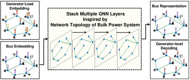
Figure 1: An Overview of the Proposed Architecture with GNN Layers. Encoders encode the input configuration vectors for generators and load units to the latent embedded vectors, then these latent embedded vectors are aggregated into the bus-level features (bus embedding). The GNN propagates the information through neighbors and produces the bus representations. Finally, the commitment decoder outputs the optimal commitment prediction for each bus.

The first component of the RACLearn framework is a novel GNN-based encoder-decoder architecture depicted in Figure 1. Let $\mathcal{B}$ be the set of bus indices, $\mathcal{G}$ the set of generator indices, $\mathcal{L}$ the set of transmission line indices, $\mathcal{D}$ the set of load demand indices, and $\mathcal{T}$ the set of time periods (commitment intervals). The ML model approximating the RAC aims at predicting commitment decisions and active transmission constraints from the problem inputs. The problem inputs include the generator and load configurations $\mathbf{g}_{g}$ and $\mathbf{l}_{l}$, detailed in Table I. It is assumed that the network topology is fixed and the difference between the instances can be described by $\mathbf{g}_{g}$ and $\mathbf{l}_{l}$, which include the forecasting of load demand and renewable generation.

The ML model can be viewed as a parametric function $F_{\theta}$, with trainable parameters $\theta$, that estimates the binary commitment decisions $\tilde{\mathbf{x}}_{g}$ and the active transmission constraints $\tilde{\mathbf{a}}_{l}$ as follows:

$$\left\{\tilde{\mathbf{x}}_{g}\right\}_{g\in\mathcal{G}},\left\{\tilde{\mathbf{a}}_{l}\right\}_{l\in\mathcal{L}}=F_{\theta}\left(\left\{\mathbf{g}_{g}\right\}_{g\in\mathcal{G}},\left\{\mathbf{l}_{l}\right\}_{l\in\mathcal{L}}\right).$$ (2)

To account for the high-dimensional and graph-structured nature of the input data $\left\{\mathbf{g}_{g}\right\}_{g\in\mathcal{G}}$, $\left\{\mathbf{l}_{l}\right\}_{l\in\mathcal{L}}$, this paper proposes a GNN-based encoder-decoder architecture. The proposed architecture consists of three parts:

1. The encoders encode the input configurations of generators and loads into the latent vectors, which are then aggregated at the bus level.

2. The core GNN layers evolve the embedded vectors at the buses, and eventually, generate bus representations.

3. The decoders outputs the optimal commitment estimates and active transmission constraint estimates.

The rest of this section discusses this architecture in detail.

V-A Encoders

Component	Name (BPM notation)	Type	Dimensions
Generator	EnergyStepWidth	continuous	$G\times T\times E$
	EnergyStepPrice	continuous	$G\times T\times E$
	EcoMinLimit	continuous	$G\times T$
	EcoMaxLimit	continuous	$G\times T$
	HotToIntTime	continuous	$G\times 1$
	HotToColdTime	continuous	$G\times 1$
	InitialOnStatus	binary	$G\times 1$
	InitialStatus	continuous	$G\times 1$
	InputRampRate	continuous	$G\times T$
	LTSCUCSDRampRate	continuous	$G\times T$
	LTSCUCSURampRate	continuous	$G\times T$
	MaxOfflineResponse	continuous	$G\times T$
	MinDownTime	continuous	$G\times 1$
	MinRunTime	continuous	$G\times 1$
	MustRunStatus	binary	$G\times T$
	NLOfferPrice	continuous	$G\times T$
	OffLineSupResOfferPrice	continuous	$G\times T$
	RF	binary	$G\times T$
	RegAvailability	binary	$G\times T$
	RegResOfferPrice	continuous	$G\times T$
	SUCOfferPrice	continuous	$G\times 1$
	SUHOfferPrice	continuous	$G\times 1$
	SUIOfferPrice	continuous	$G\times 1$
	ContResOfferPrice	continuous	$G\times T$
Load	LoadForecast	continuous	$D\times T$

TABLE I: Input Configurations for DA-FRAC and LAC. $G$ and $D$ are the number of the generators and load units, respectively. $T$ is the number of time steps, i.e., $24$ for the DA-FRAC and $12$ for the LAC.

Generator Encoder

For each generator, the input feature $\mathbf{g}$ changes from instance to instance. This input feature $\mathbf{g}$ includes the maximum capacity, pricing curve parameters, and so on. This input feature $\mathbf{g}$ is flattened to be a one-dimensional vector and embedded into a higher-dimensional latent vector $\bar{\mathbf{g}}$ through the generator encoder $\text{Enc}_{\text{g}}$, i.e., $\bar{\mathbf{g}}=\text{Enc}_{\text{g}}(\mathbf{g}).$

Load Encoder

Similarly, an input feature for each load unit $\mathbf{l}$ (i.e., the load forecast) is embedded into a latent vector $\bar{\mathbf{l}}$ using the load encoder $\text{Enc}_{\text{l}}$, i.e., $\bar{\mathbf{l}}=\text{Enc}_{\text{l}}(\mathbf{l}).$

The generator and load encoders are Multilayer Perceptron (MLP)-based structures, comprised of fully-connected layers followed by ReLU activations. The generator and load encoder structures are formulated as

$$\mathbf{h}^{(0)} =\mathbf{x},$$

$$\mathbf{\tilde{h}}^{(l)} =\mathbf{h}^{(l-1)}\mathbf{W}^{(l)}+\mathbf{b}^{(l)},$$

$$\mathbf{h}^{(l)} =\max\{\mathbf{\tilde{h}}^{(l)},0\},$$

where $\mathbf{x}$ denotes the generator or load input features. Also, at each layer $l$, $\mathbf{W}^{(l)}$ is a (trainable) weight matrix, and $\mathbf{b}^{(l)}$ is a (trainable) bias vector. Note that the trainable parameters involved in the generator and load encoders are shared across all the generators and load units, yielding an efficient structure.

Generating Bus Feature

Vectors $\bar{\mathbf{g}}$ and $\bar{\mathbf{l}}$ are then $l_{2}$-normalized, and the bus feature $\mathbf{f}_{b}\in\mathbb{R}^{d}$ at bus $b$ is defined by concatenating the sums of the generator and load features into

$$\mathbf{f}_{b}=\left[\sum_{g\in\mathcal{G}_{b}}\bar{\mathbf{g}}_{g}\middle\|\sum_{d\in\mathcal{D}_{b}}\bar{\mathbf{l}}_{d}\right],$$ (3)

where $\left[\cdot\middle\|\cdot\right]$ denotes vector concatenation, and $\mathcal{G}_{b}$ and $\mathcal{D}_{b}$ are the sets of the generator and load indices attached to bus $b$, respectively.

V-B Graph Neural Networks

Once the bus features for every bus are prepared, the whole bus features are denoted as a matrix form of $\mathbf{X}\in\mathbb{R}^{B\times d}$ where each row corresponds to the bus feature $\mathbf{f}$ and $B$ represents the number of buses in the system.

In this paper, to embed the output bus features $\mathbf{Y}$ from the input bus feature $\mathbf{X}$, two types of GNN layer are explored: GCN [50] and SIGN [51].

Graph Convolutional Network (GCN)

The power system is viewed as an unweighted undirected graph $\mathcal{N}=(\mathcal{B},\mathcal{L})$. The symmetric adjacency matrix of this graph is denoted by $\mathbf{A}\in\mathbb{R}^{B\times B}$, i.e., $A_{ij}=A_{ji}=1$ if there is a transmission line between bus $i$ and bus $j$. The self-loop added adjacency matrix $\bar{\mathbf{A}}$ is defined as $\bar{\mathbf{A}}=\mathbf{A}+\mathbf{I}$.

A GCN layer typically utilizes the normalized adjacency matrix $\tilde{\mathbf{A}}$ defined as: $\tilde{\mathbf{A}}=\mathbf{D}^{-1/2}\bar{\mathbf{A}}\mathbf{D}^{-1/2}$, where $\mathbf{D}$ is the degree matrix, i.e., $\mathbf{D}=\text{diag}(\sum_{j=1}^{B}\bar{A}_{1j},\dots,\sum_{j=1}^{B}\bar{A}_{Bj})$. The GCN propagates the information to the neighbor nodes along the edge using graph diffusion operations. Given the matrix form of the input bus features $\mathbf{X}\in\mathbb{R}^{B\times d}$, the $d^{\prime}$-dimensional output bus features $\mathbf{Y}\in\mathbb{R}^{B\times d^{\prime}}$ is obtained as

$$\mathbf{Y}=\text{GCN}(\mathbf{X}|\tilde{\mathbf{A}})=\sigma\left(\tilde{\mathbf{A}}\mathbf{X}\bm{\Theta}\right),$$

where $\sigma(\cdot)$ represents the ReLU activation, and $\bm{\Theta}\in\mathbb{R}^{d\times d^{\prime}}$ is a matrix of trainable parameters.

The GCN layer only propagates messages to neighboring nodes, i.e., 1-hop neighbors. To propagate the message throughout the network, a multiple GCN layers stacked structure can be utilized. Using bus embedding $\mathbf{H}^{(l-1)}\in\mathbb{R}^{B\times d^{(l-1)}}$ as the input of $l^{th}$ GCN layer, the output is given by

$$\mathbf{H}^{(l)}=\text{GCN}_{l}(\mathbf{H}^{(l-1)}|\tilde{\mathbf{A}})=\sigma\left(\tilde{\mathbf{A}}\mathbf{H}^{(l-1)}\bm{\Theta}^{(l)}\right),$$

where $\bm{\Theta}^{(l)}\in\mathbb{R}^{d^{(l-1)}\times d^{(l)}}$ is trainable parameters of the layer $l$ and $\mathbf{H}^{(0)}=\mathbf{X}$. Then, the output of the final GCN layer $\mathbf{H}^{(L)}$ of the $L$-stacked GCN structure is regarded as the output bus feature $\mathbf{Y}$. It is still an open question whether a multiple-stacked GNN structure gives an enhanced performance in general [51]. Thus, recent research has utilized different types of diffusion operators to replace the normalized adjacency matrix and allow messages to propagate beyond 1-hop neighbors [52, 53]. For instance, S-GCN [52] employs the $p^{th}$ power of the normalized adjacency matrix to encompass $p$-hop neighbors in its propagation, i.e., S-GCN is defined as

$$\mathbf{Y}=\sigma\left(\tilde{\mathbf{A}}^{p}\mathbf{X}\bm{\Theta}\right).$$

Scalable Inception Graph Neural Network (SIGN)

Another type of GNN layer, SIGN [51], uses Inception-like architecture [54] on graph-structured data, and generalizes the use of various diffusion operators in the GCN structure. In particular, SIGN concatenates multiple output bus features from various diffusion operators. In addition to the use of the adjacency matrix that only covers the spatial domain, the SIGN architecture considered in this paper uses the personalized PageRank (PPR) based spectral diffusion operator $\mathbf{S}$ [53] and its powers. The SIGN layer can be formalized as

$$\mathbf{Y}=\sigma\left(\text{MLP}\left(\xi\left(\bigparallel_{i=1}^{p}\text{GCN}(\mathbf{X}|\tilde{\mathbf{A}}^{i}),\bigparallel_{i=1}^{s}\text{GCN}(\mathbf{X}|\mathbf{S}^{i})\right)\right)\right),$$

where $\xi$ and $\sigma$ are nonlinear activation functions. In practice, PReLU and ReLU have been used for $\xi$ and $\sigma$, respectively. Also, MLP denotes fully connected layers followed by ReLU activations. $p$ and $s$ are hyperparameters representing the maximum powers used to construct representational features in parallel for the normalized adjacency matrix and the PPR diffusion operator, respectively. The details on the PPR diffusion operator are provided in Appendix C.

V-C Decoders

Denote the output bus feature of bus $j$ from the GNN as $\bar{\mathbf{f}_{j}}$, which corresponds to the $j^{th}$ row of $\mathbf{Y}$. It remains to estimate the optimal commitment decisions and active transmission constraints.

Commitment Decoder

Since multiple generators can be located at the same bus, another generator encoder (independent and distinct from the previous generator encoder) is used to generate another embedded vector $\dot{\mathbf{g}}$. This vector is concatenated to the bus features $\bar{\mathbf{f}_{j}}$ (with $i\in\mathcal{G}_{j}$) to obtain a generator-level representation $\tilde{\mathbf{g}_{i}}$, i.e., $\tilde{\mathbf{g}}_{i}=\left[\bar{\mathbf{f}}_{j}\middle\|\dot{\mathbf{g}}_{i}\right]$, Then, the MLP-based commitment decoder $\text{Dec}_{\text{g}}$ uses $\tilde{\mathbf{g}_{i}}$ as an input and outputs a $|\mathcal{T}|$-dimensional vector $\tilde{\mathbf{x}}_{i}$ that represents the commitment decision likelihood for the generator $i$, i.e., $\tilde{\mathbf{x}}_{i}=\text{Dec}_{\text{g}}(\tilde{\mathbf{g}}_{i})$. The $t^{th}$ element of $\tilde{\mathbf{x}}_{i}$ represents the probability of committing generator $i$ at time step $t\in\mathcal{T}$, This value is the output of a sigmoid function attached to the final layer of the decoder $\text{Dec}_{\text{g}}$.

Transmission Decoder

The vector $\mathbf{e}_{l}$ of transmission line $l$, linking buses $i$ and $j$, can be represented by the permutation-invariant element-wise summation of the associated output bus-representations, i.e., $\mathbf{e}_{l}=\bar{\mathbf{f}}_{i}+\bar{\mathbf{f}}_{j}.$ The MLP-based transmission decoder $\text{Dec}_{\text{t}}$ uses vector $\mathbf{e}_{l}$ to estimate whether the transmission constraints are tight or not, i.e., $\tilde{\mathbf{a}}_{l}=\text{Dec}_{\text{t}}(\mathbf{e}_{l})$ for all transmissions $l\in\mathcal{L}$. Note that $\tilde{\mathbf{a}}$ is a $2|\mathcal{T}|$ dimensional vector where $2$ comes from the lower and upper limits of each transmission constraint. Like the commitment decoders, $\tilde{\mathbf{a}}_{l}$ represents the sigmoid-based binary probabilities that the transmission constraints of transmission $l$ are active.

VI Confidence Measurement

The second component of the RACLearn framework is the confidence measurement of the prediction. Unlike other critical applications such as semantic segmentation for self-driving AI [55] or medical image diagnosis [56], ML approaches in power systems have not been extensively studied through the lens of uncertainty quantification. The RACLearn framework remedies this limitation and provides an epistemic uncertainty-based confidence measure for each output of the ML model. Specifically, to quantify the confidence in each commitment prediction, RACLearn exploits MC-dropout [46], one of the popular tools to measure epistemic uncertainty (also called model uncertainty) by approximating a Bayesian neural network [45]. A dropout layer, at training time, chooses nodes at random, and sets the trainable parameters associated with those nodes to zero in order to prevent overfitting during training. The dropout layer is also used at inference to express the stochasticity involved in the input data. That is, instead of providing a single prediction, MC-dropout generates $T$ of them. The mean $\mu$ of these $T$ predictions is then used as the output prediction, while the variance $\sigma$ serves as a proxy for the epistemic uncertainty, i.e.,

$$\mu(\tilde{x})=\frac{1}{T}\sum_{t=1}^{T}\tilde{x}^{(t)},$$

$$\sigma(\tilde{x})=\frac{1}{T-1}\sqrt{\sum_{t=1}^{T}\left(\tilde{x}^{(t)}-\mu(\tilde{x})\right)},$$

When the model is to estimate on unseen or unfamiliar input instances, $\sigma$ tends to be higher, representing the higher epistemic uncertainty involved in the prediction from the model. Thus, the confidence measure, which has the reciprocal relationship with the epistemic uncertainty, can be defined as

$$\text{Conf}(\tilde{x}):=\frac{1}{\sigma(\tilde{x})}.$$ (5)

RACLearn generates confidence values for the commitment of each generator at each time step. The implementation attaches a dropout layer with a dropout probability of $0.5$ to the penultimate layer of the commitment decoder.

VII The Predict-Repair-Optimize Heuristic

The last component of the RACLearn framework is the feasibility restoration. It is motivated by a key challenge faced in solving RAC (or SCUC in general): to find high-quality feasible solutions quickly [6, 49]. RACLearn addresses this challenge with Predict-Repair-Optimize heuristic involving the feasibility restoration step, which is guaranteed to return a feasible solution. The Predict-Repair-Optimize heuristic consists of four components; 1) estimating the active transmission constraints and add at the beginning of the iterative optimization procedure, 2) fixing generator commitments with high confidence, 3) executing the feasibility restoration step to repair the fixed commitments, and 4) solving the reduced RAC problem w.r.t. the remaining continuous variables.

VII-A Estimating Active Transmission Constraints

The first step in the Predict-Repair-Optimize heuristic is to estimate the active transmission constraints. Figure 2 highlights that few transmission constraints are active in an optimal RAC solution. This justifies the use of the iterative optimization procedure [10] that first solves the relaxed problem where there is no transmission constraints and then adds violated transmission constraints lazily until there is no violation. To accelerate the optimization procedure, akin to the approach suggested in [13], it is desirable to estimate the active likely transmission constraints and add those constraints at the beginning of the iterative procedure in order to decrease the number of iterations. Again, the transmission decoder generates a sigmoid-based binary probability as its output to estimate the activeness of a transmission constraint.

VII-B Fixing Generator Commitments

The second step of the Predict-Repair-Optimize heuristic fixes the binary variables corresponding to confident commitment decisions. The confidence level needed to fix the commitment decisions is a hyper-parameter that is studied in Section VIII.

VII-C Feasibility Restoration

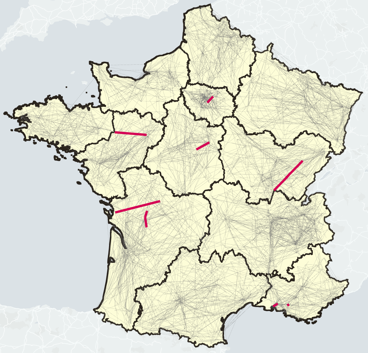
Figure 2: Active Transmission Constraints in the RAC Solution. The red thick lines represent the active constraints, whereas grey thin lines show non-active transmission constraints.

Fixing confident commitments may result in an infeasible RAC problem instance. Specifically, the prediction $\tilde{\mathbf{x}}$ may conflict with the commitment-level constraints (1b) in the RAC formulation. To address this issue, the RACLearn framework repairs the prediction $\tilde{\mathbf{x}}$ to obtain commitment decisions $\hat{\mathbf{x}}$ that satisfy (1b). Then, the commitment decisions are fixed to $\hat{\mathbf{x}}$, and the RAC is re-optimized, yielding $\hat{\mathbf{y}}$ such that $(\hat{\mathbf{x}},\hat{\mathbf{y}})$ is feasible for Problem (1). The rest of this section describes the repair step and proves that it runs in polynomial times.

Let $\tilde{\mathbf{x}}$ be the optimal commitment estimates to a RAC instance. This prediction does not guarantee that $\tilde{\mathbf{x}}$ will satisfy the combinatorial constraints (1b). To alleviate this issue, the paper introduces a repair step which, akin to a projection step, seeks a feasible $\hat{\mathbf{x}}\in\mathcal{X}$ that is close to $\tilde{\mathbf{x}}$. Formally, the repair step solves

$$\hat{\mathbf{x}}\in\arg\min_{\mathbf{x}}\quad \mathcal{H}(\mathbf{x},\tilde{\mathbf{x}})$$ (6a)

s.t. $$\mathbf{x}\in\mathcal{X},$$ (6b)

where $\mathcal{H}(\mathbf{x},\tilde{\mathbf{x}})$ is the Hamming distance between $\mathbf{x}$ and $\tilde{\mathbf{x}}$.

Theorem 1.

Problem (6) can be solved in polynomial time.

Proof.

First, because commitment constraints are formulated at the generator level, Problem (6) can be decomposed into $G$ single-generator problems, where $G$ is the number of generators. Second, because $\mathbf{x},\tilde{\mathbf{x}}$ are binary vectors, objective (6a) is linear. Thus, Problem (6) reduces to optimizing a linear objective over the commitment constraints for a single generator. This is solvable in polynomial time using the dynamic-programming algorithm of Frangioni and Gentile [57]. ∎

Theorem 2.

The Predict-Repair-Optimize heuristic returns a feasible solution $(\hat{\mathbf{x}},\hat{\mathbf{y}})$ in polynomial time.

Proof.

By Theorem 1, a feasible $\hat{\mathbf{x}}$ can be obtained in polynomial. Then, recall that constraints (1d) are soft. In addition, the structure of constraints (1c) is such that, for any $\mathbf{x}$ that satisfies (1b), there exists a vector $\mathbf{y}$ that satisfies (1c). For instance, it suffices to set the reserve dispatch of each generator to zero, and its energy dispatch to its minimum output at every time period. Finally, once the binary variables $\mathbf{x}$ are fixed, Problem (1) reduces to a linear program, which can be solved in polynomial time to obtain $\hat{\mathbf{y}}$. ∎

VIII Experimental Results

VIII-A Experimental Settings

VIII-A1 The Case Studies

Experiments were conducted on the RTE system in France. The system contains 8965 transmission lines and 6708 buses where 1890 generators and 6262 load units are located. Solar/wind power generation and load demand forecast were obtained through LSTM-based models [58] trained on the publicly-available ground truth obtained from RTE [59]. The stochastic forecast scenarios are generated via MC-dropout [46]. Supply offer bids were synthetically generated by the approach proposed in [60].

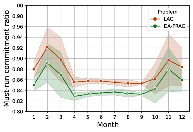
Figure 3: Ratio of the Must-run Commitments ($x_{gh}^{\text{prev}}=1$) in DA-FRAC and LAC Instances. The shaded region represents the standard deviation.

Two distinct types of RAC problems are studied: DA-FRAC and LAC. For gathering DA-FRAC instances, the DA market (DA-SCUC) is first executed. The must-run commitments for the DA-FRAC are then extracted from the DA-SCUC solution. For gathering LAC instances, the DA-FRAC is first executed and the must-run commitments are extracted from its solution. A LAC instance is solved every 15 minutes and it uses all the commitment decisions of the DA-FRAC and prior LAC executions as the must-run commitments. Figure 3 shows that the majority of the commitment decisions are already determined by prior optimization decisions. Ratios of the must-run commitments are above 80% and 85% for DA-FRAC and LAC, respectively.

VIII-A2 Data Generation

The formulations of the DA-FRAC, LAC, and DA-SCUC were modeled with JuMP [61] and solved through Gurobi 9.5 [62]. To gather the instances, the optimizations were solved on Linux machines in the PACE Phoenix cluster at Georgia Tech [63]. The data instances are gathered by setting the optimality gap to $0.1\%$ and using 2 threads and $8GB$ RAM. The time limit was set to 3600 seconds and the parameter MIPFocus was set to 1 for focusing on finding feasible solutions. The remaining parameters use the default values. Only the instances with the optimal solutions that are obtained within the time limit are included in the dataset for stable training. When generating instances, transmission constraints are added in an iterative manner as suggested in [10]. The solution process starts with no transmission constraints. At each iteration, the 15 most violated transmission constraints are added into the formulation sequentially until no violations are observed.

The number of data instances for each month is around 9000 for the DA-FRAC and 8600 for the LAC. The training and testing procedures are performed on a monthly basis, i.e., the training is performed on data instances of a month, and the testing is conducted on the data instances of the following month. Thus, in 2018, 11 independent models for each month (February to December) are trained and tested. Note that this experimental setting inherently features a distribution shift [64], since the data distributions of the training and testing datasets are different. It mimics the natural way of deploying the models in real-world settings, using historical data to infer the upcoming commitment decisions. For each month of training, 100 instances are extracted and used for validation. 1000 testing instances are also sampled from the next month’s instances for measuring and reporting the performance results.

VIII-A3 Training Configuration

The proposed GNN-based architecture and other neural network baselines were implemented and trained using PyTorch. The proposed architecture is trained in an end-to-end manner by minimizing binary cross-entropy loss with respect to the commitment estimates and active transmission constraint estimates in a supervised way. The minibatch size was set to 8 for training. The AdamW optimizer [65] with a learning rate of $1\mathrm{e}{-4}$ and a weight decay of $1\mathrm{e}{-6}$ was used for updating the trainable parameters. Early stopping was applied with a the patience of 5, while the learning rate decayed by $0.95$ when the validation loss was worse than the best validation loss at every epoch. The maximum epoch was set to 20. The training and testing process was performed using Tesla V100 GPU on machines with Intel CPU cores at 2.7GHz. The architectural design of the proposed GNN-based encoder-decoder structure is detailed in Appendix A. Other details on the training process are elaborated in Appendix B.

VIII-B Commitment Prediction Accuracy

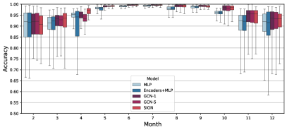
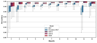
Figure 4: Monthly Performance for DA-FRAC (Left) and LAC (Right).

This section reports the performance of the optimal commitment predictions of the proposed GNN-based models as well as various baselines. The RACLearn framework was tested with several GNN layers: While the encoder and decoder structures remain the same for every architecture, the GNN layers to propagate bus representations are different: they are SIGN, GCN-1 (a single GCN layer), and GCN-5 (5 stacked GCN layers).

VIII-B1 Baselines

The RACLearn architectures are compared to two neural network baselines: MLP has three fully-connected layers of 512 hidden nodes and flattens all the input features; Encoders+MLP uses the encoder structures of RACLearn, flattens the embedded generator/load features, and applies 3 fully-connected layers, followed by ReLU activations, with 512 hidden nodes instead of using the GNN and decoder structures of RACLearn.

The RACLearn framework is also compared to the following shallow models taken from scikit-learn [66]. SVM-poly is an SVM model with a polynomial kernel, SVM-rbf is an SVM model with radial basis function-based kernel, and RF is a random-forest model. All those shallow models use the default parameter settings. Those shallow models are not scalable to the case study and hence a naïve autoencoder (AE) was used to decrease the dimensionality of the input feature space. AE has three MLP layers for each encoder and decoder. The encoder embedding vector has a dimensionality of 0.2% of that of the input features. The number of hidden nodes is set to the mean of dimensions of the input and embedding features. This AE model is also trained using the AdamW optimizer with a learning rate of $5\mathrm{e}{-5}$ up to 20 epochs with a minibatch of 16 instances. When training, must-run commitments are masked out to focus on the non-must-run commitments.

VIII-B2 Accuracy Results

Model	Accuracy	AUROC
SVM-poly	0.895(0.692,0.951)	0.853(0.650,0.960)
SVM-rbf	0.898(0.674,0.949)	0.855(0.651,0.961)
RF	0.896(0.702,0.949)	0.860(0.645,0.968)
MLP	0.960(0.907,0.992)	0.870(0.626,0.955)
Encoders+MLP	0.960(0.905,0.993)	0.870(0.626,0.955)
GCN-1	0.981(0.915,0.996)	0.869(0.748,0.976)
GCN-5	0.980(0.915,0.996)	0.892(0.742,0.983)
SIGN	0.981(0.914,0.996)	0.905(0.776,0.990)

TABLE II: Overall Accuracy and AUROC Performance Results for DA-FRAC. The bounds of the 95% confidence intervals are presented between parenthesis. The best values are in bold.

Model	Accuracy	AUROC
SVM-poly	0.913(0.666,0.949)	0.916(0.640,0.958)
SVM-rbf	0.912(0.692,0.951)	0.883(0.664,0.961)
RF	0.916(0.733,0.948)	0.905(0.683,0.961)
MLP	0.982(0.966,0.991)	0.965(0.678,0.986)
Encoders+MLP	0.986(0.973,0.991)	0.980(0.839,0.993)
GCN-1	0.994(0.990,0.998)	0.995(0.975,1.000)
GCN-5	0.994(0.990,0.998)	0.995(0.973,0.999)
SIGN	0.994(0.990,0.998)	0.995(0.976,0.999)

TABLE III: Overall Accuracy and AUROC Performance Results for LAC. The bounds of the 95% confidence intervals are presented between parenthesis. The best values are in bold.

The prediction results for DA-FRAC and LAC are depicted in Tables II and III. The tables report the mean accuracy together with 95% confidence intervals. The metrics are calculated using bootstrapping with 1000 samples from the testing set with replacement. The performance measures are the averaged accuracy and the area under the receiver operating characteristic curve (AUROC). In all cases, GNN-based models are superior to the swallow and MLP-based models in terms of accuracy and AUROC. There is no significant difference in performance among the GNN-based models. The prediction accuracy is higher for the LAC than for the DA-FRAC, which is explained by the smaller variability in forecasts and the shorter time horizon of the LAC.

Figure 4 depicts the monthly performance of the models (the shallow models are excluded because of their poor performances). It highlights that the winter season (from October to March) is more challenging to predict and has more outliers. The figure also indicates that the GNN-based architectures outperform their MLP-based counterparts by a significant margin.

Initially, it was anticipated that SIGN would exhibit superior performance compared to other GNN-based architectures, as SIGN leverages more comprehensive operators to distill information from the entire power grid’s features. However, the results indicate that there are no notable distinctions among GNN-based architectures. This can be attributed to the fact that the power grid can be characterized as a small-world network [67], where most nodes can be reached from every node with a limited number of hops. As such, the generation commitment can be estimated with the localized features; the loads and the generator’s features from neighboring nodes, rather than from distant nodes.

VIII-C Commitment Prediction Confidence

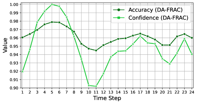
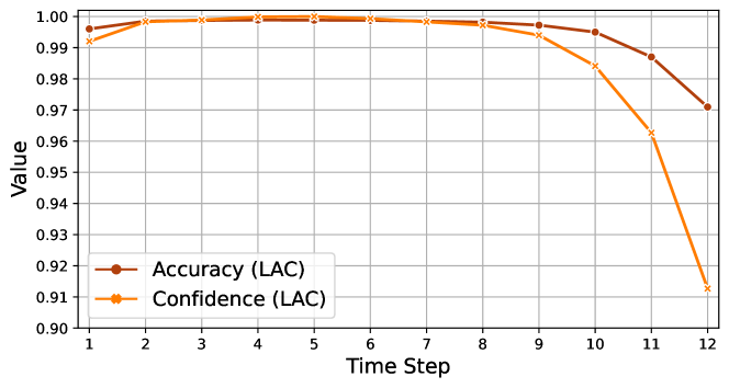
Figure 5: Average Testing Accuracy and Associated Confidence Values for the Commitment Decisions at Each Time Step of DA-FRAC (Top) and the LAC (Bottom). Confidence values are normalized (i.e., divided by the maximum confidence value).

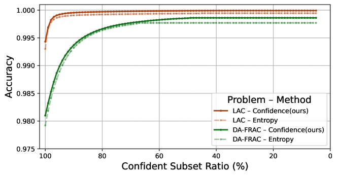
Figure 6: Performance on the Confident Subsets and Whole Set. The x-axis shows the ratio of the number of commitments in the confident subset divided by the total number of commitments (denoted in percentage). Confidence used in this work is compared with the entropy measure.

Among the GNN-based models, the SIGN model was chosen for the rest of the experiments. Figure 5 shows the average testing accuracy and its corresponding normalized confidence values from Eq. (5) of the commitment predictions at each time step for the DA-FRAC and the LAC. Recall that the numbers of time steps for the DA-FRAC and the LAC are 24 and 12. For the LAC, the accuracy of the predictions decreases as the time step increases. This comes from the fact that the LAC is run over a rolling horizon during operations. Earlier steps have more must-run commitments and more accurate forecasts. For the DA-FRAC, each instance predicts the next day, the forecasts for each hour are more consistent, and fewer must-run commitments are imposed. In this case, the accuracy is consistent within the range between $0.95$ and $0.99$. Interestingly, in both cases, the confidence value is high and in agreement with the accuracy. For instance, in LAC, the average confidence value at step 12 is significantly lower than other steps, which is indicative of less accurate results. This is confirmed by the accuracy results. Note that the confidence value is obtained without relying on the ground truth.

The RACLearn framework uses commitment predictions to fix binary variables, reducing the dimensionalities of these optimization problems. Moreover, the confidence values associated with the predictions provide valuable information about which predictions must be used in this process in order to balance the quality of the solutions and the dimensionality reduction. Using lower confidence predictions may deteriorate the quality of the solutions, while only using the predictions with the highest confidence may not provide significant computational benefits. Figure 6 explores this trade-off. The x-axis captures the percentage of highly confident commitment predictions selected to fix variables in the optimization models, which is called the confident subset. The y-axis captures the average accuracy of the selected predictions. The percentages are ranked in decreasing order in Figure 6: a percentage of 100% means that all the predictions will be used; a percentage of 30% means that the confident subset consists of the 30% of predictions with the highest confidence values. The figure shows how fast the average accuracy increases monotonically as the size of the confident subset decreases for both the FRAC and the LAC cases. For the LAC, the accuracy can increase to around $1.000$ as soon as the confident subset contains less than 50% of the predictions. Similarly, for the DA-FRAC, the accuracy increases to around $0.998$ if low-confident commitment estimates are rejected, whereas when all commitment estimates are concerned, the accuracy was $0.981$. These predictions based on the MC-dropout-based confidence measure are likely to be accurate, leading to an attractive tradeoff between solution quality and dimensionality reduction in the reduced optimization.

Figure 6 also includes the binary entropy (denoted as Entropy) for comparison. This measure is directly induced by the softmax-based probability [40], which has been utilized in the previous ML-based approaches in power system applications [14, 13]. The figure shows that the proposed confidence measure (based on MC-dropout) performs better than the binary entropy to classify the confident subset. This coincides with the comparison results in [56] in the medical domain.

VIII-D Prediction of Active Transmission Constraints

Problem	Method	Recall$\uparrow$	#Pred Pos.$\downarrow$	#Pos.
DA-FRAC	Baseline	0.822(0.057)	965.24	125.29
	RACLearn	0.914(0.063)	409.91
LAC	Baseline	0.979(0.008)	242.46	70.94
	RACLearn	0.981(0.034)	141.18

TABLE IV: Recall Performance of Active Transmission Constraint Prediction. Column #Pred Pos. represents the averaged number of predicted active transmission constraints. Column #Pos. denotes the averaged number of actual active transmission constraints.

Actual unit-commitment problems have few active transmission constraints and previous works have shown that they can be predicted with reasonable accuracy by identifying those transmissions [68, 13]. To evaluate the performance of the RACLearn framework in predicting active constraints, this paper adopts baselines that exploit prior runs of the RAC model, i.e., the FRAC of the previous day or the LAC that was run 15 minutes before. In the baseline, all the constraints are considered active if they are included in a transmission line that had at least one active constraint in the prior run. In RACLearn, transmission constraint predictions with above 0.1 probability are regarded as being active.

Table IV presents experimental results showing the benefits of predicting active constraints compared to the baselines. Those predictions are expected to obtain high recall values while having a small number of active constraint predictions. The recall value, i.e., the true positive rate, is the fraction of correctly predicted active constraints among all constraints that are actually active. The recall value is an appropriate measure because the false negatives (the constraints predicted as not active, but active actually) should be added to the formulation subsequently, which leads to excessive time for solving the problem.

On average, there are about 125 active constraints in the DA-FRAC and 71 in the LAC. On average, the baseline isolates 965.24 constraints (DA-FRAC) and 242.46 constraints (LAC) that can be active for recall values of 0.822 (DA-FRAC) and 0.979 (LAC). In contrast, RACLearn identifies 409.91 (DA-FRAC) and 141.18 (LAC) possible active constraints on average. The recall values are 0.914 and 0.981 for the DA-FRAC and LAC, respectively. Hence, compared to the baseline, RACLearn provides better recall values (especially for the DA-FRAC) and adds fewer constraints to the optimization model, demonstrating its practical value. More detailed results are included in Appendix D.

VIII-E Optimization Speedups

				CPU time
Method	%Fixed†	Feas(%)	Gap(%)	Total(s)	Scaled‡
DA-FRAC
Baseline	–	100.00	0.00	126.06	1.00
RACLearn w/o feasibility restoration	30	100.00	0.01	48.93	0.38
	50	100.00	0.02	47.56	0.37
	70	100.00	0.06	45.07	0.35
	90	89.61	0.07	35.82	0.30
	100	31.17	0.12	19.19	0.25
RACLearn	30	100.00	0.01	48.40	0.38
	50	100.00	0.02	47.36	0.37
	70	100.00	0.06	45.03	0.35
	90	100.00	0.16	38.81	0.30
	100	100.00	0.77	31.56	0.24
LAC
Baseline	–	100.00	0.00	42.71	1.00
RACLearn w/o feasibility restoration	30	100.00	0.00	26.44	0.62
	50	100.00	0.00	25.08	0.59
	70	99.53	0.01	25.04	0.59
	90	98.59	0.01	21.87	0.51
	100	84.51	0.09	21.59	0.53
RACLearn	30	100.00	0.00	25.45	0.60
	50	100.00	0.00	24.82	0.58
	70	100.00	0.01	23.67	0.56
	90	100.00	0.01	22.73	0.53
	100	100.00	0.09	20.94	0.49

^†percentage of commitments fixed in RACLearn.
^‡relative to baseline. CPU Time is computed on the feasible instances.

TABLE V: Optimization Speedup Performance of the RACLearn Framework. The baseline is the optimization baseline using [10]; the RACLearn performances are reported for various confidence levels of the commitment estimates fixed (shown in column %Fixed). Column Feas represents the fraction of the feasible instances. Column Gap represents the geometric mean of the optimization gaps. Column Total is the geometric mean of the CPU running times.

The results for the optimization speedups are reported in Table V. The baseline is the iterative optimization procedure [10] with $k=15$ (adding 15 transmission constraints at each iteration of the overall procedure) as suggested in [13]. According to [69], at MISO, the DA-FRAC and LAC have to be solved within 40 and 10 minutes. The results in elapsed times of the baseline for DA-FRAC and LAC are $126.06$ and $42.71$ seconds. These times are higher than those obtained for the MISO system because the RTE system is significantly larger and more congested in general. For RACLearn, Table  V reports the results when the confident subset contains 0%, 30%, 50%, 70%, 90%, and 100% of the predictions. For the LAC, the results show that enforcing the predictions (even all of them) incurs only a small loss in solution quality, e.g., 0.01% for 90% of the predictions and 0.09% for 100%. Moreover, the computing times are reduced by about 50%. For the DA-FRAC, committing up to 90% of the predictions results in a small quality loss and reduces the execution times by more than a factor of 3. It reduces the execution times by a factor of more than 4, if a quality loss of $0.77\%$ is acceptable.

If the feasibility restoration step is not included in the RACLearn framework, fixing the commitment predictions could produce infeasible solutions. In fact, when all commitment variables are fixed to their predictions, only 31.17% of instances are feasible for the DA-FRAC cases. The feasibility restoration step, which takes polynomial time, transforms infeasible solutions into feasible solutions with a slightly worse optimality gap for the DA-FRAC. For the LAC, the feasibility restoration does not affect the optimality gap significantly.

It is important to emphasize that the optimization speedup results rely on the three components of RACLearn: the commitments of generators for which the predictions are highly confident, the predictions of the active transmission constraints, and the feasibility restoration. More detailed results on the quality/performance tradeoffs and the role of each component are given in Appendix E.

IX Conclusion

This paper proposed the RACLearn framework to speed up the solving of RAC problems and, in particular, the DA-FRAC and LAC. RACLearn consists of three key components: (1) a dedicated GNN-based architecture to predict generator commitments and active transmission lines; (2) the use of the GNN-based architecture and MC-dropout to associate a confidence value to each commitment prediction; and (3) a feasibility-restoration procedure that transforms the prediction into a high-quality feasible solution in polynomial time. Experimental results on the French transmission system and the DA-FRAC and LAC formulations used by MISO indicate that RACLearn can provide significant speedups in solving for negligible loss in solution quality. The RACLearn framework sheds light on the use of confidence measurement and uncertainty quantification in ML approaches to power systems. Future research will explore how to further improve the confidence calibration and the architectural design of the GNNs. The RACLearn framework can be generalized to the stochastic optimization versions of the FRAC and the LAC. Additionally, this framework can be further enhanced to address network topology changes, thereby extending its applicability to accelerate optimal transmission planning or generalize transmission contingencies.

Appendix A Details on the Learning Architectures

Problem	Component	Encoder Name	Input Dim.	Output Dim.
DA-FRAC	Generator	Continuous generator encoder	249	176
		Binary generator encoder	55	32
		Energy generator encoder	480	16
	Load	Load encoder	24	32
LAC	Generator	Continuous generator encoder	141	176
		Binary generator encoder	43	32
		Energy generator encoder	240	16
	Load	Load encoder	12	32

TABLE VI: Input/output dimensions of the generator and load encoders for DA-FRAC and LAC

Encoders

The architecture proposed in Section V is described here in detail. The generator encoder $\text{Enc}_{g}$ can be separated into three components; binary encoder, continuous encoder, and energy encoder. The binary encoder only encodes the binary type input configurations to the latent representations. Similarly, the continuous encoder encodes the continuous input configuration parameters. The energy encoder encodes the energy step width and price to the latent representations. The reasons for having three separable encoders for the generator are as follows. First, it allows for a reduction in the number of trainable parameters associated with the MLP structures. Indeed, given $n$ dimensional input features, the number of trainable parameters between two consecutive fully-connected layers is $n^{2}$, which can be reduced to $3\left(\frac{n}{3}\right)^{2}$ when the input features are equally separated to three encoders. Second, the input configurations for the energy step width and price are quite sparse; most of the values are zero, meaning those have less information. Thus, the energy encoder is designed to output a smaller dimensional latent feature than other encoders. Third, trainable parameters for the binary features and continuous features can be affected by each other, thus for better normalization of the weight parameters associated with fully-connected layers, the encoders for binary and continuous features should be separated. Table VI illustrates the dimensions for each binary/continuous/energy input configuration parameters per generator as well as for a load unit. Note that all the trainable parameters of the encoders are shared for all generators and load units. All the encoders are comprised of MLP structures. A continuous generator encoder has $3$ fully-connected layers, whereas others have $2$ fully-connected layers. All the fully-connected layers are followed by one-dimensional batch normalization [70] and a ReLU activation. The number of hidden nodes for all the encoders are the average of the input and output dimensions. Specifically, the nodes for the binary generator encoder are $55-43-32$ and $43-37-32$ for the DA-FRAC and LAC, respectively. Here, the first and last numbers represent, respectively, input and output feature dimensions. The number of nodes for the energy generator encoder are $480-248-16$, and $240-128-16$ for the DA-FRAC and LAC, respectively. The number of nodes for the continuous generator encoder are $249-212-212-176$ and $141-158-158-176$ for the DA-FRAC and LAC, respectively. The output dimension of the encoders is $176+32+32+16=256$ for both cases.

Graph Neural Networks

The GCN-1 architecture uses one GCN layer where the weight has $256\times 256$ trainable parameters. GCN-5 contains five GCN layers that also output a 256-dimensional vector. SIGN has $5$ GCN layers with the normalized adjacency matrix and $3$ GCN layers with the diffusion operator. Each GCN layer outputs a 64-dimensional vector, thus the associated trainable parameters form a $256\times 64$ dimensional matrix. The eight output vectors of individual GCN layers are concatenated and processed by two-layered MLP. The number of nodes for this MLP is $8\times 64-384-256$, and the MLP produces a 256-dimensional vector for each bus of the network structure.

Decoders

The commitment decoder is also an MLP structure with bus configurations of the form $256-210-210-24$, and $256-201-201-12$ for the DA-FRAC and LAC, respectively. Each layer is followed by a ReLU activation. A dropout layer with a dropout probability of $0.5$ is attached at the penultimate layer and is used to measure the confidence of the predictions. Note that the output dimension corresponds to the number of time steps. The sigmoid is attached to the output of the commitment decoder to furnish the probability of committing each generator. The number of nodes for the transmission line decoder are the same as those for the commitment decoder. Each layer is also followed by a ReLU activation.

Total Number of Trainable Parameters

Problem	Model	# Trainable Parameters
DA-FRAC	MLP	859,143,472
	Encoders+MLP	133,980,184
	GCN-1	1,159,896
	GCN-5	1,423,064
	SIGN	2,177,369
LAC	MLP	460,670,104
	Encoders+MLP	122,039,458
	GCN-1	818,733
	GCN-5	1,081,901
	SIGN	1,871,078

TABLE VII: The Number of Trainable Parameters of the Models for DA-FRAC and LAC.

The number of total trainable parameters of the proposed GNN-based architectures and the other two deep baselines are summarized in Table VII. As shown in the table, the number of trainable parameters of the GNN-based architectures is much smaller than that of the dense baselines. This is critical to scale to realistic networks.

Appendix B Details on Training

Denote by $\mathbf{p}$ the input configuration vector that contains the generator input features and load input features for all generators and loads. Denote by $\mathbf{x}^{*}\in\{0,1\}$ the ground-truth optimal commitment decisions that are obtained by solving the optimization problems. The optimal commitment decisions $\mathbf{x}^{*}$ is a $|\mathcal{G}|\!\times\!|\mathcal{T}|$ dimensional matrix in which an element $x_{gt}^{*}$ corresponds to the optimal commitment decision for the generator $g$ at time step $t$. For each generator, recall that there are some must-run commitments, i.e., $x_{gt}^{\text{prev}}=1$ that do not need to be predicted as they are determined by previous commitment decisions.

For instance $i$ and the commitment estimation $\tilde{\mathbf{x}}$ produced by the ML model, the commitment loss function $L_{c}$ minimized during training is the binary cross entropy between $\tilde{\mathbf{x}}$ and $\mathbf{x}^{*}$ defined as

$$L_{c}^{(i)}=-\sum_{\begin{subarray}{c}g\in\mathcal{G},t\in\mathcal{T}\\ |x_{gt}^{\text{prev}}=0\end{subarray}}x_{gt}^{*(i)}\log\tilde{x}_{gt}^{(i)}+(1-x_{gt}^{*(i)})\log(1-\tilde{x}_{gt}^{(i)}).$$

Similarly, if the ground-truth transmission constraint is given by $\mathbf{a}^{*}$ where 1 represents being active, the transmission loss function is defined as

$$L_{t}^{(i)}=-\sum_{t\in\mathcal{L}^{\prime}}a_{t}^{*(i)}\log\tilde{a}_{t}^{(i)}+(1-a_{t}^{*(i)})\log(1-\tilde{a}_{t}^{(i)}),$$

where $\mathcal{L}^{\prime}$ comprises of active transmission constraints and some samples of non active transmission constraints, called negative sampling [71], which is widely used in natural language processing. The use of $\mathcal{L}^{\prime}$ instead of whole transmission set $\mathcal{L}$ is due to the sparsity of active transmissions and maintaining the balance between two classes.

Given $N$ instances in the training dataset, the loss function can be defined as

$$L=\frac{1}{N}\sum_{i=1}^{N}\left(L_{c}^{(i)}+\lambda L_{t}^{(i)}\right),$$ (7)

where $\lambda$ is a hyper-parameter to balance between the two loss terms. By minimizing the loss function (7) with respect to the trainable parameters, the estimations for commitment decisions and active transmission constraints are obtained simultaneously in an end-to-end manner. In the experiments, $\lambda$ is set to $1$ for training.

Appendix C Details on the Diffusion Operator

The generalized graph diffusion matrix used in this study is defined as follows [53]:

$$\mathbf{S}=\sum_{i=0}^{\infty}\theta_{k}\tilde{\mathbf{A}}^{k},$$ (8)

with the weighting coefficients $\theta_{k}$ and the normalized adjacency matrix. The weighting coefficients should ensure that $\sum_{k=0}^{\infty}\theta_{k}=1$ and $\theta_{k}\in[0,1]$. The personalized PageRank (PPR) based diffusion operator exploits $\theta_{k}=\alpha(1-\alpha)^{k}$ with teleport probability $\alpha\in(0,1)$ to satisfy the aforementioned requirements. Because of the boundedness of the eigenvalues of $\tilde{\mathbf{A}}$ and the property of the geometric series, the closed form of the PPR-based diffusion operator can be obtained as

$$\mathbf{S}=\sum_{i=0}^{\infty}\alpha(1-\alpha)^{k}\tilde{\mathbf{A}}^{k}=\alpha\left(\mathbf{I}_{N}+(\alpha-1)\tilde{\mathbf{A}}\right)^{-1},$$ (9)

where $\mathbf{I}_{N}$ is the $N\times N$ identity matrix. Note that $\mathbf{S}$ is now a dense matrix, and should be sparsified to represent the spacial locality using the top-$k$ parameter. The sparse diffusion operator with the top-$k$ parameter distills the $k$ highest entries per column and other entries are set to zero. In the experiment, top-$k$ parameter is set to $256$.

Appendix D Performance Results on Active Transmission Line Constraints

Month	Acc.	AUPR	AUROC	Pos. Ratio	#Pos.
DA-FRAC
Feb.	0.9982(0.0012)	0.3462(0.1619)	0.9548(0.0586)	0.0008(0.0003)	350.4200(142.2894)
Mar.	0.9994(0.0004)	0.2494(0.1485)	0.9515(0.0721)	0.0005(0.0004)	232.3700(173.6947)
Apr.	0.9999(0.0001)	0.5571(0.1935)	0.9901(0.0111)	0.0001(0.0000)	45.2240(16.8886)
May	0.9999(0.0000)	0.5571(0.1935)	0.9901(0.0111)	0.0001(0.0000)	45.2240(16.8886)
June	1.0000(0.0000)	0.9223(0.0652)	0.9985(0.0047)	0.0001(0.0000)	42.4920(12.1598)
July	1.0000(0.0000)	0.7566(0.1136)	0.9875(0.0132)	0.0001(0.0000)	39.1666(10.8016)
Aug.	0.9999(0.0000)	0.8103(0.1137)	0.9887(0.0196)	0.0001(0.0000)	47.5480(15.3757)
Sep.	1.0000(0.0000)	0.8048(0.1365)	0.9867(0.0300)	0.0001(0.0000)	24.3260(9.7112)
Oct.	0.9999(0.0002)	0.4794(0.3129)	0.8826(0.1153)	0.0001(0.0002)	47.2500(69.4714)
Nov.	0.9994(0.0006)	0.2611(0.1493)	0.9317(0.0496)	0.0005(0.0003)	211.7900(140.1693)
Dec.	0.9991(0.0006)	0.4230(0.1056)	0.9820(0.0115)	0.0007(0.0004)	304.0460(160.2599)
Total	0.9996(0.0007)	0.5400(0.2857)	0.9672(0.0592)	0.0003(0.0004)	125.2884(152.1879)
LAC
Feb.	0.9989(0.0006)	0.5621(0.1656)	0.9703(0.0583)	0.0008(0.0003)	164.6520(71.6983)
Mar.	0.9994(0.0006)	0.5436(0.1899)	0.9948(0.0336)	0.0005(0.0007)	107.5860(143.1241)
Apr.	0.9999(0.0001)	0.5026(0.3421)	0.9985(0.0063)	0.0001(0.0001)	19.6750(15.7187)
May	0.9999(0.0000)	0.5883(0.3719)	0.9971(0.0129)	0.0001(0.0001)	26.6875(20.1051)
June	1.0000(0.0000)	0.8631(0.2637)	0.9476(0.1336)	0.0001(0.0001)	27.2336(21.2843)
July	0.9999(0.0000)	0.6861(0.3249)	0.9985(0.0093)	0.0001(0.0001)	28.1809(24.4316)
Aug.	0.9999(0.0000)	0.7415(0.3088)	0.9946(0.0319)	0.0002(0.0001)	33.9729(27.2578)
Sep.	1.0000(0.0000)	0.7104(0.3599)	0.9881(0.0637)	0.0001(0.0001)	21.4605(20.8516)
Oct.	0.9999(0.0003)	0.4614(0.3618)	0.9598(0.0651)	0.0002(0.0003)	36.5758(55.1402)
Nov.	0.9994(0.0007)	0.5904(0.2037)	0.9611(0.0611)	0.0005(0.0005)	105.9457(110.6117)
Dec.	0.9994(0.0004)	0.6168(0.1343)	0.9936(0.0083)	0.0007(0.0003)	143.2720(69.7454)
Total	0.9997(0.0005)	0.6178(0.2993)	0.9818(0.0594)	0.0003(0.0004)	70.9388(88.5095)

TABLE VIII: Performance Results on Active Transmission Constraints in DA-FRAC and LAC. Accuracy (Acc.), area under precision-recall curve (AUPR), and area under receiver operating characteristic curve (AUROC) are presented as performance measures. The standard deviations are shown in parenthesis. Pos. Ratio represents the ratio of the positive labels (active transmissions) and #Pos is the averaged number of active transmissions in each test instance. The results are obtained from 500 instances per month.

The classification performance for active transmission constraints is reported in Table VIII for RAC optimizations. The results are based on SIGN that is also used for reporting the commitment decision performance and speedup results. The results are calculated using 500 test instances per each test month from February to December in 2018. More transmission lines are congested in the winter, leading to a higher number of active transmission lines compared to the summer season. This also makes it harder to predict the active transmission constraints in the winter, mirroring the results for commitment decisions in Fig 4.

The proportion of the active transmission constraints is quite unbalanced, which is around $0.03\%$ for both RACs. Accuracy (Acc.) and AUROC values are relatively high, but those are not adequate measure to denote the performance for imbalanced classification problems. Instead, the area under precision recall curve (AUPR) is the best choice as a measure of classification performance. The baseline AUPR value in this case with a randomized classifier is $0.0003$, which is the same as the ratio of the positive labels. Recall that the prediction of active transmission is less sensitive than commitment decisions. Note that RACLearn could adds false negative predictions in the iterative optimization procedure. These false negative lines do not affect the feasibility of the optimization model, but slow the solver down slightly.

Appendix E Detailed Results on the Optimization Speedups

TABLE IX: Speedup Ablation Study for DA-FRAC. The speedup performances of the proposed approach are denoted in bold.

ADD1	#Added	FIX2	Ratio(%)	FR3	Feasibility(%)	Opt.Gap(%)	Times(s)	Speedup
✗	-	✗	-	✗	100.00	0.00	126.06	1.0000$\times$
✓	147.12	✗	-	✗	100.00	0.00	61.15	2.0581$\times$
✗	-	✓	30	✗	100.00	0.01	94.56	1.3595$\times$
			50		100.00	0.02	91.19	1.4074$\times$
			70		100.00	0.06	83.99	1.5261$\times$
			90		89.61	0.07	63.75	1.8471$\times$
			100		31.17	0.12	32.19	2.4268$\times$
✓	147.12	✓	30	✗	100.00	0.01	48.93	2.6267$\times$
			50		100.00	0.02	47.56	2.6938$\times$
			70		100.00	0.06	45.07	2.8405$\times$
			90		89.61	0.07	35.82	3.2800$\times$
			100		31.17	0.12	19.19	4.0674$\times$
✓	147.12	✓	30	✓	100.00	0.01	48.40	2.6571$\times$
			50		100.00	0.02	47.36	2.7078$\times$
			70		100.00	0.06	45.03	2.8436$\times$
			90		100.00	0.16	38.81	3.3135$\times$
			100		100.00	0.77	31.56	4.1160$\times$

1) ADD: whether to add active transmission constraints prediction at the beginning of the iterative optimization.
2) FIX: whether to fix highly confident commitment decisions to their predictions.
3) FR: whether to use feasibility restoration.

TABLE X: Speedup Ablation Study for LAC. The speedup performances of the proposed approach are denoted in bold.

ADD	#Added	FIX	Ratio(%)	FR	Feasibility(%)	Opt.Gap(%)	Times(s)	Speedup
✗	-	✗	-	✗	100.00	0.00	42.71	1.0000$\times$
✓	119.94	✗	-	✗	100.00	0.00	29.11	1.4472$\times$
✗	-	✓	30	✗	100.00	0.00	35.97	1.2143$\times$
			50		100.00	0.01	34.79	1.2577$\times$
			70		99.53	0.01	32.93	1.3293$\times$
			90		98.58	0.01	30.97	1.4030$\times$
			100		84.91	0.09	25.96	1.6445$\times$
✓	119.94	✓	30	✗	100.00	0.00	26.44	1.6012$\times$
			50		100.00	0.00	25.08	1.6987$\times$
			70		99.53	0.01	25.04	1.6844$\times$
			90		98.59	0.01	21.87	1.9460$\times$
			100		84.51	0.09	21.59	1.8772$\times$
✓	119.94	✓	30	✓	100.00	0.00	25.45	1.6719$\times$
			50		100.00	0.00	24.82	1.7086$\times$
			70		100.00	0.01	23.67	1.8018$\times$
			90		100.00	0.01	22.73	1.8781$\times$
			100		100.00	0.09	20.94	2.0585$\times$

This Appendix analyzes the contributions of each component of RACLearn to the speedups reported in Section VIII-E. It shows that the learning benefits for commitments and active constraints are cumulative. It also shows that feasibility restoration is critical in practice.

The experiments consider four settings for the confident subset: 30%, 50%, 70%, or 90% of the highly confident commitment predictions. For example, in the 30% confident subset, 30% of highly confident commitments will be fixed to their predictions. For the active transmission constraints, RACLearn adds to the optimization algorithm all constraints whose probability of being active is greater than $0.1$ are added to the beginning of the iterative optimization procedure. This is a conservative threshold but it is counteracted by the fact that RACLearn only add at most $400$ constraints.

The results of speedup with some components ablated are depicted in Table IX and Table X for the DA-FRAC and the LAC. In the experiments, 20 instances per month are drawn at random from the monthly test dataset from February to December. The optimality gap (represented as Opt. Gap in tables) is calculated as the geometric mean of relative differences in objective values between the baseline and reduced problem divided by the baseline objective value on the feasible instances. To treat some negative values when calculating the geometric mean, 0.1% is used as a shift value. Also, the time and speedup columns in the tables represent the geometric means of elapsed times for solving the optimization instances and their fractions based on the baseline case.

The baseline (denoted as ‘ADD’, ‘FIX’, and ‘FR’ with ✗) is the iterative method [10] with $k=15$ as suggested in [13]. According to [69], at MISO, the DA-FRAC and LAC must be solved within 40, 10 minutes. The elapsed times of the baseline iterative method for DA-FRAC and LAC is $126.06$ and $42.71$ seconds, respectively, which are around 14-20 times faster than the time limits, meaning that the baseline is quite competitive.

The second row of the result of the tables (denoted as ‘ADD’:✓, ‘FIX’:✗, ‘FR’:✗) shows the computational results when only the active constraint predictions are considered. It is important to note that these predictions do not affect the feasibility of the optimization, since the algorithm will add active constraints as needed. The predictions only affect the running times by reducing the number of iterations. The addition of transmission constraints results in speedups of $2.0581\!\times$ and $1.4472\!\times$ for the DA-FRAC or the LAC, respectively. The total number of the transmission constraints is $2\!\times\!8965\!\times\!24=430,320$ and $2\!\times\!8965\!\times\!12=215,160$ for the DA-FRAC and the LAC, (the $2$ comes from the min/max bounds). The number of added transmission constraints (denoted as ‘#Added’ in the tables) at the beginning of the iterative method is relatively small; $147.12$ or $119.94$ for the DA-FRAC and the LAC in average. By adding around $0.02$-$0.06\%$ of the transmission constraints at the beginning of the iterative optimization procedure, speedups of around $40$-$100\%$ can be obtained over the baseline.

The next lines in the table reports result when only generator commitment predictions are used (the FIX column), which is denoted as ‘ADD’:✗, ‘FIX’:✓, ‘FR’:✗ in the tables. Fixing $90\%$ of highly confident commitment predictions leads to speedups of $1.8471\times$, $1.4030\times$ for the DA-FRAC and the LAC. However, about 10% of the instances become infeasible in the DA-FRAC when doing so. The infeasibility issue is especially severe when fixing all the predictions.

The next results consider the case where both the commitment predictions and the active constraint predictions are used together. This is represented by (‘ADD’:✓, ‘FIX’:✓, ‘FR’:✗). The main result here is that the speedups are cumulative, especially for the DA-FRAC. The infeasibilies are still present obviously.

The last set of lines adds the feasibility restoration to obtain the RACLearn framework (denoted by (‘ADD’:✓, ‘FIX’:✓ and ‘FR’:✓) in the table). Feasibility restoration marginally increases the optimality gaps in general and the RACLearn framework speeds up the optimization by factor of about 4 and 2 for the DA-FRAC and the LAC.

References

- [1] CEC. (2022) New data indicates california remains ahead of clean electricity goals. [Online]. Available: https://www.energy.ca.gov/news/2022-02/new-data-indicates-california-remains-ahead-clean-electricity-goals
- [2] X. Ma, H. Song, M. Hong, J. Wan, Y. Chen, and E. Zak, “The security-constrained commitment and dispatch for midwest iso day-ahead co-optimized energy and ancillary service market,” in 2009 IEEE Power & Energy Society General Meeting. IEEE, 2009, pp. 1–8.
- [3] Y. Chen, V. Ganugula, J. Williams, J. Wan, and Y. Xiao, “Resource transition model under miso mip based look ahead commitment,” in 2012 IEEE Power and Energy Society General Meeting. IEEE, 2012, pp. 1–8.
- [4] Y. Chen, Q. Wang, X. Wang, and Y. Guan, “Applying robust optimization to miso look-ahead commitment,” in 2014 IEEE PES General Meeting— Conference & Exposition. IEEE, 2014, pp. 1–5.
- [5] MISO, “Reliability assessment commitment software formulations and business logic,” Oct-15-2021, business Practices Manual, Energy and Operating Reserve Markets Attachment C, BPM-002-r22.
- [6] Y. Chen, A. Casto, F. Wang, Q. Wang, X. Wang, and J. Wan, “Improving large scale day-ahead security constrained unit commitment performance,” IEEE Transactions on Power Systems, vol. 31, no. 6, pp. 4732–4743, 2016.
- [7] K. Pan and Y. Guan, “A polyhedral study of the integrated minimum-up/-down time and ramping polytope,” arXiv preprint arXiv:1604.02184, 2016.
- [8] P. Damcı-Kurt, S. Küçükyavuz, D. Rajan, and A. Atamtürk, “A polyhedral study of production ramping,” Mathematical Programming, vol. 158, no. 1, pp. 175–205, 2016.
- [9] J. Ostrowski, M. F. Anjos, and A. Vannelli, “Tight mixed integer linear programming formulations for the unit commitment problem,” IEEE Transactions on Power Systems, vol. 27, no. 1, pp. 39–46, 2011.
- [10] A. S. Xavier, F. Qiu, F. Wang, and P. R. Thimmapuram, “Transmission constraint filtering in large-scale security-constrained unit commitment,” IEEE Transactions on Power Systems, vol. 34, no. 3, pp. 2457–2460, 2019.
- [11] K. Kim, A. Botterud, and F. Qiu, “Temporal decomposition for improved unit commitment in power system production cost modeling,” IEEE Transactions on Power Systems, vol. 33, no. 5, pp. 5276–5287, 2018.
- [12] M. J. Feizollahi, M. Costley, S. Ahmed, and S. Grijalva, “Large-scale decentralized unit commitment,” International Journal of Electrical Power & Energy Systems, vol. 73, pp. 97–106, 2015.
- [13] A. S. Xavier, F. Qiu, and S. Ahmed, “Learning to solve large-scale security-constrained unit commitment problems,” INFORMS Journal on Computing, vol. 33, no. 2, pp. 739–756, 2021.
- [14] A. V. Ramesh and X. Li, “Feasibility layer aided machine learning approach for day-ahead operations,” arXiv preprint arXiv:2208.06742, 2022.
- [15] X. Tang, X. Bai, Z. Weng, and R. Wang, “Graph convolutional network-based security-constrained unit commitment leveraging power grid topology in learning,” Energy Reports, vol. 9, pp. 3544–3552, 2023.
- [16] M. I. A. Shekeew and B. Venkatesh, “Learning-assisted variables reduction method for large-scale milp unit commitment,” IEEE Open Access Journal of Power and Energy, 2023.
- [17] A. Velloso and P. Van Hentenryck, “Combining deep learning and optimization for preventive security-constrained dc optimal power flow,” IEEE Transactions on Power Systems, vol. 36, no. 4, pp. 3618–3628, 2021.
- [18] X. Pan, T. Zhao, M. Chen, and S. Zhang, “Deepopf: A deep neural network approach for security-constrained dc optimal power flow,” IEEE Transactions on Power Systems, vol. 36, no. 3, pp. 1725–1735, 2020.
- [19] X. Pan, T. Zhao, and M. Chen, “Deepopf: Deep neural network for dc optimal power flow,” in 2019 IEEE International Conference on Communications, Control, and Computing Technologies for Smart Grids (SmartGridComm). IEEE, 2019, pp. 1–6.
- [20] A. S. Zamzam and K. Baker, “Learning optimal solutions for extremely fast ac optimal power flow,” in 2020 IEEE International Conference on Communications, Control, and Computing Technologies for Smart Grids (SmartGridComm). IEEE, 2020, pp. 1–6.
- [21] B. Donon, Z. Liu, W. Liu, I. Guyon, A. Marot, and M. Schoenauer, “Deep statistical solvers,” Advances in Neural Information Processing Systems, vol. 33, pp. 7910–7921, 2020.
- [22] F. Cengil, H. Nagarajan, R. Bent, S. Eksioglu, and B. Eksioglu, “Learning to accelerate globally optimal solutions to the ac optimal power flow problem,” Electric Power Systems Research, vol. 212, p. 108275, 2022.
- [23] S. Park and P. Van Hentenryck, “Self-supervised primal-dual learning for constrained optimization,” arXiv preprint arXiv:2208.09046, 2022.
- [24] F. Fioretto, T. W. Mak, and P. Van Hentenryck, “Predicting ac optimal power flows: Combining deep learning and lagrangian dual methods,” in Proceedings of the AAAI Conference on Artificial Intelligence, vol. 34, no. 01, 2020, pp. 630–637.
- [25] M. Chatzos, F. Fioretto, T. W. Mak, and P. Van Hentenryck, “High-fidelity machine learning approximations of large-scale optimal power flow,” arXiv preprint arXiv:2006.16356, 2020.
- [26] M. Chatzos, T. W. Mak, and P. Vanhentenryck, “Spatial network decomposition for fast and scalable ac-opf learning,” IEEE Transactions on Power Systems, 2021.
- [27] W. Chen, S. Park, M. Tanneau, and P. Van Hentenryck, “Learning optimization proxies for large-scale security-constrained economic dispatch,” Electric Power Systems Research, vol. 213, p. 108566, 2022.
- [28] K. Baker, “Learning warm-start points for ac optimal power flow,” in 2019 IEEE 29th International Workshop on Machine Learning for Signal Processing (MLSP). IEEE, 2019, pp. 1–6.
- [29] L. Chen and J. E. Tate, “Hot-starting the ac power flow with convolutional neural networks,” arXiv preprint arXiv:2004.09342, 2020.
- [30] F. Diehl, “Warm-starting ac optimal power flow with graph neural networks,” in 33rd Conference on Neural Information Processing Systems (NeurIPS 2019), 2019, pp. 1–6.
- [31] D. Deka and S. Misra, “Learning for dc-opf: Classifying active sets using neural nets,” in 2019 IEEE Milan PowerTech. IEEE, 2019, pp. 1–6.
- [32] A. Robson, M. Jamei, C. Ududec, and L. Mones, “Learning an optimally reduced formulation of opf through meta-optimization,” arXiv preprint arXiv:1911.06784, 2019.
- [33] F. Hasan, A. Kargarian, and J. Mohammadi, “Hybrid learning aided inactive constraints filtering algorithm to enhance ac opf solution time,” IEEE Transactions on Industry Applications, vol. 57, no. 2, pp. 1325–1334, 2021.
- [34] K. Baker, “A learning-boosted quasi-newton method for ac optimal power flow,” arXiv preprint arXiv:2007.06074, 2020.
- [35] S. Zeng, A. Kody, Y. Kim, K. Kim, and D. K. Molzahn, “A reinforcement learning approach to parameter selection for distributed optimization in power systems,” arXiv preprint arXiv:2110.11991, 2021.
- [36] Y. Tang, S. Agrawal, and Y. Faenza, “Reinforcement learning for integer programming: Learning to cut,” in International Conference on Machine Learning. PMLR, 2020, pp. 9367–9376.
- [37] E. Khalil, H. Dai, Y. Zhang, B. Dilkina, and L. Song, “Learning combinatorial optimization algorithms over graphs,” Advances in neural information processing systems, vol. 30, 2017.
- [38] V. Nair, S. Bartunov, F. Gimeno, I. von Glehn, P. Lichocki, I. Lobov, B. O’Donoghue, N. Sonnerat, C. Tjandraatmadja, P. Wang et al., “Solving mixed integer programs using neural networks,” arXiv preprint arXiv:2012.13349, 2020.
- [39] D. Owerko, F. Gama, and A. Ribeiro, “Optimal power flow using graph neural networks,” in ICASSP 2020-2020 IEEE International Conference on Acoustics, Speech and Signal Processing (ICASSP). IEEE, 2020.
- [40] D. Hendrycks and K. Gimpel, “A baseline for detecting misclassified and out-of-distribution examples in neural networks,” arXiv preprint arXiv:1610.02136, 2016.
- [41] D. P. Kingma, T. Salimans, R. Jozefowicz, X. Chen, I. Sutskever, and M. Welling, “Improved variational inference with inverse autoregressive flow,” Advances in neural information processing systems, vol. 29, 2016.
- [42] M. Germain, K. Gregor, I. Murray, and H. Larochelle, “Made: Masked autoencoder for distribution estimation,” in International Conference on Machine Learning. PMLR, 2015, pp. 881–889.
- [43] S. Park and P. M. Pardalos, “Deep data density estimation through donsker-varadhan representation,” arXiv preprint arXiv:2104.06612, 2021.
- [44] S. Liang, Y. Li, and R. Srikant, “Enhancing the reliability of out-of-distribution image detection in neural networks,” arXiv preprint arXiv:1706.02690, 2017.
- [45] Y. Gal et al., “Uncertainty in deep learning,” 2016.
- [46] Y. Gal and Z. Ghahramani, “Dropout as a bayesian approximation: Representing model uncertainty in deep learning,” in international conference on machine learning. PMLR, 2016, pp. 1050–1059.
- [47] S. Park, G. Adosoglou, and P. M. Pardalos, “Interpreting rate-distortion of variational autoencoder and using model uncertainty for anomaly detection,” Annals of Mathematics and Artificial Intelligence, pp. 1–18, 2021.
- [48] B. Knueven, J. Ostrowski, and J.-P. Watson, “On mixed-integer programming formulations for the unit commitment problem,” INFORMS Journal on Computing, vol. 32, no. 4, pp. 857–876, 2020.
- [49] Y. Chen, F. Pan, F. Qiu, A. Xavier, T. Zheng, P. Luh, B. Yan, M. Bragin, H. Zhong, F. F. Li et al., “Security-constrained unit commitment for electricity market: Modeling, solution methods, and future challenges,” 2022.
- [50] T. N. Kipf and M. Welling, “Semi-supervised classification with graph convolutional networks,” arXiv preprint arXiv:1609.02907, 2016.
- [51] E. Rossi, F. Frasca, B. Chamberlain, D. Eynard, M. Bronstein, and F. Monti, “Sign: Scalable inception graph neural networks,” arXiv preprint arXiv:2004.11198, 2020.
- [52] F. Wu, A. Souza, T. Zhang, C. Fifty, T. Yu, and K. Weinberger, “Simplifying graph convolutional networks,” in International conference on machine learning. PMLR, 2019, pp. 6861–6871.
- [53] J. Klicpera, S. Weißenberger, and S. Günnemann, “Diffusion improves graph learning,” arXiv preprint arXiv:1911.05485, 2019.
- [54] C. Szegedy, W. Liu, Y. Jia, P. Sermanet, S. Reed, D. Anguelov, D. Erhan, V. Vanhoucke, and A. Rabinovich, “Going deeper with convolutions,” in Proceedings of the IEEE conference on computer vision and pattern recognition, 2015, pp. 1–9.
- [55] A. Kendall and Y. Gal, “What uncertainties do we need in bayesian deep learning for computer vision?” Advances in neural information processing systems, vol. 30, 2017.
- [56] C. Leibig, V. Allken, M. S. Ayhan, P. Berens, and S. Wahl, “Leveraging uncertainty information from deep neural networks for disease detection,” Scientific reports, vol. 7, no. 1, pp. 1–14, 2017.
- [57] A. Frangioni and C. Gentile, “Solving nonlinear single-unit commitment problems with ramping constraints,” Operations Research, vol. 54, no. 4, pp. 767–775, 2006.
- [58] S. Hochreiter and J. Schmidhuber, “Long short-term memory,” Neural computation, vol. 9, no. 8, pp. 1735–1780, 1997.
- [59] RTE. (2022) eco2mix - all of france’s electricity data in real time. [Online]. Available: https://www.rte-france.com/en/eco2mix
- [60] M. Chatzos, M. Tanneau, and P. Van Hentenryck, “Data-driven time series reconstruction for modern power systems research,” Electric Power Systems Research, vol. 212, p. 108589, 2022.
- [61] I. Dunning, J. Huchette, and M. Lubin, “Jump: A modeling language for mathematical optimization,” SIAM Review, vol. 59, no. 2, pp. 295–320, 2017.
- [62] Gurobi Optimization, LLC, “Gurobi Optimizer Reference Manual,” 2021. [Online]. Available: https://www.gurobi.com
- [63] PACE, Partnership for an Advanced Computing Environment (PACE), 2017. [Online]. Available: http://www.pace.gatech.edu
- [64] J. Quiñonero-Candela, M. Sugiyama, A. Schwaighofer, and N. D. Lawrence, Dataset shift in machine learning. Mit Press, 2008.
- [65] I. Loshchilov and F. Hutter, “Decoupled weight decay regularization,” arXiv preprint arXiv:1711.05101, 2017.
- [66] F. Pedregosa, G. Varoquaux, A. Gramfort, V. Michel, B. Thirion, O. Grisel, M. Blondel, P. Prettenhofer, R. Weiss, V. Dubourg, J. Vanderplas, A. Passos, D. Cournapeau, M. Brucher, M. Perrot, and E. Duchesnay, “Scikit-learn: Machine learning in Python,” Journal of Machine Learning Research, vol. 12, pp. 2825–2830, 2011.
- [67] D. J. Watts and S. H. Strogatz, “Collective dynamics of ‘small-world’networks,” nature, vol. 393, no. 6684, pp. 440–442, 1998.
- [68] L. A. Roald and D. K. Molzahn, “Implied constraint satisfaction in power system optimization: The impacts of load variations,” in 2019 57th Annual Allerton Conference on Communication, Control, and Computing (Allerton). IEEE, 2019, pp. 308–315.
- [69] N. Barry, M. Chatzos, W. Chen, D. Han, C. Huang, R. Joseph, M. Klamkin, S. Park, M. Tanneau, P. Van Hentenryck et al., “Risk-aware control and optimization for high-renewable power grids,” arXiv preprint arXiv:2204.00950, 2022.
- [70] S. Ioffe and C. Szegedy, “Batch normalization: Accelerating deep network training by reducing internal covariate shift,” in International conference on machine learning. PMLR, 2015, pp. 448–456.
- [71] T. Mikolov, I. Sutskever, K. Chen, G. S. Corrado, and J. Dean, “Distributed representations of words and phrases and their compositionality,” Advances in neural information processing systems, vol. 26, 2013.