CWD: A Machine Learning based Approach to Detect Unknown Cloud Workloads

Abstract

Workloads in modern cloud data centers are becoming increasingly complex. The number of workloads running in cloud data centers has been growing exponentially for the last few years, and cloud service providers (CSP) have been supporting on-demand services in real-time. Realizing the growing complexity of cloud environment and cloud workloads, hardware vendors such as Intel and AMD are increasingly introducing cloud-specific workload acceleration features in their CPU platforms. These features are typically targeted towards popular and commonly-used cloud workloads. Nonetheless, uncommon, customer-specific workloads (unknown workloads), if their characteristics are different from common workloads (known workloads), may not realize the potential of the underlying platform. To address this problem of realizing the full potential of the underlying platform, we develop a machine learning based technique to characterize, profile and predict workloads running in the cloud environment. Experimental evaluation of our technique demonstrates good prediction performance. We also develop techniques to analyze the performance of the model in a standalone manner.

I Introduction

Workloads in modern cloud data centers are becoming increasingly complex. Moreover, the number of such workloads is growing at an unprecedented rate. Data Center Industry Survey Results, published by Uptime Institute in 2019 [1] found that although the majority of IT workloads are still on enterprise data centers, data center workloads are becoming both complex and extensive. More importantly, it also found that cloud capacity is growing at a faster rate than the capacity of the enterprise data center and that IT workloads continue to move to the cloud. For instance, software-development paradigms are transitioning from monolithic applications to smaller, finer-grained, and distributed services (microservices), and cloud service providers (CSP) have started offering serverless computing platforms that bill resources at finer granularities (e.g., Function-as-a-services (FaaS)). For example, NetFlix and Salesforce are increasingly adopting cloud-native principles (e.g., cloud-native functions, which is a type of microservice) and architectural design principles to support on-demand services. New specific-purpose models, such as FaaS, add to the complexity of cloud environments that are already supporting more general-purpose models such as infrastructure-as-a-service (IaaS), software-as-a-service (SaaS), platform-as-a-service (PaaS). In addition to workload complexity, even the deployment models are becoming more complex. Specifically, workload consolidation — co-locating different workloads to drive up utilization and improve efficiently (e.g., energy efficiency) — is a common model in most of the public clouds now. At the hardware level, resource disaggregation is a popular approach to avoid resource stranding in data centers.

Realizing the growing trend of workload migration to cloud and the need of accelerating growing diversity of cloud workloads, hardware vendors such as Intel and AMD already offer several performance-oriented features in their cloud-specific platforms. For instance, Intel’s recently launched 3rd generation Xeon Scalable processors are routinely used in cloud environments, and they offer several features (e.g., Intel Total Memory Encryption that protects data and VMs by encrypting their physical memory, Intel Crypto Acceleration that accelerates commonly-used hash functions and encryption protocols, etc.) that accelerate common cloud workloads. Such platform features, when combined with software optimizations, accelerate commonly-used, popular cloud workloads and microservices.

One of the common problems faced by hardware vendors in cloud environments is the inability to analyze performance bottlenecks and resource utilization of cloud workloads. This is partly because of the fact that the hardware vendors have limited access in cloud environments; typically, they have access limited access at the hardware level, let alone the software stack. Lack of such analysis makes it difficult to evaluate impact of different hardware features on workload performance. Operating within such a constrained environment, in this paper, we attempt to answer a question of if it is possible to identify the workload running on a given system in cloud. To answer this question, we develop a machine learning (ML) based system, named CWD (Cloud Workload Detection), that utilizes hardware performance counters to develop workload fingerprints and then employs an efficient approach to compare fingerprints to detect unknown workloads. Intuitively, fingerprint of a workload is its unique signature that distinguishes the execution of that workload from others. Our experimental results demonstrate efficacy of CWD in detecting unknown workloads with a high degree of accuracy.

Although, we do not discuss possible applications of detecting unknown cloud workloads in this paper, it is not difficult to imagine a number of applications. For instance, one can propose possible optimizations to the unknown workload, if the performance of that workload is lower than its expected performance on the hardware platform (e.g., a crypto workload is not using crypto acceleration engine in the hardware). Another application could be of enabling privacy-preserving analysis of cloud workloads — the hardware vendors could apply the approach described in this paper to identify a proxy workload that has similar fingerprint as that of a proprietary cloud workload and then analyze the proxy workload instead of the actual workload.

II Related work

As a new cloud workload continuously emerge, designing and deploying a reliable physical computer hardwares in a data center are extremely vital. The hardware includes storage, networking, processor, memory and etc. Furthermore, without evaluating, analyzing and identifying the characteristics and profile of a workload running in a cloud, it is very difficult to optimize and improve the performance of that workload. To solve this problem, many researchers have proposed various methods. Khanna et al. developed [2] a workload phase forecasting method to evaluate and analyze the run-time behavior of workloads in a cloud. The results obtained that the new model of workload phase shows that 98% accurate in phase identification and 97.15% accurate in forecasting the compute demands. In addition, Jandaghi et al. [3] studied workload profile and resource usage prediction technique to detect a workload in Apache Spark framework using a gaussian mixture model. Furthermore, Elnaffar et al. [4] introduced a new model that characterizing a workload. As the author noted that the method helps to evaluate and predict workload performance. Bhattacharyya et al. [5] proposed a performance modeling technique for cloud workload to evaluate and predict workloads performance by identifying automatically workload phases. The results showed that this method can predict the performance of applications with up to 95% accuracy for previously unseen input configurations at less than 5% overhead. Moreover, [6] introduced for automatic phase detection and characterization applications running in a cloud. The results achieved detecting a phases upto 98.2% accuracy with an average detection delay of less than 0.01 seconds. Besides, Sherwood et al. [7] introduced a unified profiling architecture to capture, classify, and predict phase-based program behavior of workloads. Furthermore, Calheiros et al. [8] presented a cloud workload prediction model for cloud service providers using the autoregressive integrated moving average (ARIMA). As Desprez et al. [9] has proposed that a workload prediction based on a similar past occurrences of the current short-term workload history; present an overall evaluation of this approach and usefulness for enabling efficient auto-scaling of cloud resources.

We develop a machine learning based technique to characterize, profile and predict workloads running in a cloud environment. Experimental evaluation of our technique demonstrates good prediction performance. We also develop techniques to analyze the performance of the model in a standalone manner.

The rest of the paper is laid out as follows.The first section describes the background information, prior art, and related work done in the domain of workload characterization and analysis, workload profile methodologies, and workload phase detection methods. The following section includes a theoretical description of the machine learning methodology and phase classification, phase evaluation, correlation changepoint detection, and probabilistic and statistical models for phase-different workload. The experiment section includes our setup and analysis of observed result data from real dataset. The fourth section proposes the result and analysis. Finally, the conclusion and future work are discussed in the last section.

III Algorithms

In this paper, we combine three algorithms to predict unknown workload running in a cloud: a) change point detection, b) Euclidean distance and c) dynamic time warping (DTW)

III-A Change Point Detection

Change point detection technique can be used to locate the transition between phases or states in a signal or time-series data[13]. The occurrence of the state depends on some underlying dynamic change on the system. For example, when a noise is added into a signal or time series data (hardware and software performance counters), it causes an abrupt change to the sequence of a signal or time series data. The detection of abrupt change(change points) in a signal or time series data is a well studied problem, several authors have proposed several techniques such as outlier detection, relative density ratio estimation and etc. In this research, we use a multivariate change point detection method to identify the state transitions of a time series data for hardware and software performance counters such as L1 cache misses, LLC cache misses, CPU utilization, iTLB misses, etc.

III-A1 Problem Formulation

we assume that the sequence of observations can be expressed as $y_{1:n}$$=(y_{1}$, $y_{2,\cdots,}$$y_{n}$)^T denote $n$ data samples observed. Each data samples lies in $R^{d}$ and $y_{n}$$\epsilon$ $\mathbb{R^{d}}$, $\forall$ $n$$=1,2,\cdots,N.$ Note that $d$ is a dimensional space records hardware and software counter data. $y_{i:j}$ represents the data between time indices $i$ and $j$, where $(y_{i}$,$y_{i+1,\cdots,}$$y_{j}$)^T. In this case, there is some $M$ change points in time series data points sequence, denoted in increasing order based on the following indices such as $t_{1}$,…,$t_{m}$ and let $t_{0}$$=0$ and $t_{M+1}$$=N$. To identify the transition between phases, we apply Bayesian Change Point Detection(BCPD) algorithm[14] which is based on Bayes’ rule [15] that describes the probability of a prior distribution and likelihood distribution and computes the posterior distribution $p\left(x_{t}\mid y_{1:t}\right)$ as shown equation (5).

$$p\left(x_{t}\mid y_{1:t}\right)=\frac{p(y_{1:t}\mid x_{t})\centerdot p(x_{t})}{p(y_{1:t})}$$ (1)

Where $p(x_{t})$ is a vector and prior observation of hardware and software counters of time series data and $x_{t}$ is the run length of the change point detection algorithm. $p(y_{1:t}\mid x_{t})$ is a vector and the current observation and the joint likelihood distribution of hardware and software counters of time series data. The joint likelihood distribution is computed based on each new observation of the counters. We can express the joint distribution over run length and observed data recursively.

$$p\left(x_{t}\mid y_{1:t}\right) =\sum p(x_{t},x_{t-1},y_{1:t})$$ (2)

$$=\sum p(x_{t},y_{t}\mid x_{t-1,}y_{1:t-1})p(x_{t-1},y_{1:t-1})$$ (3)

$$=\sum p(x_{t},x_{t-1})p(y_{t}\mid x_{t-1,}y_{t}^{(x)})p(x_{t-1},x_{1:t-1})$$ (4)

As equ. (4) shows that based on the newly observed and prior data point, the posterior distribution predicts the new change point of a multivariate time series data of hardware and software performance counters.

Moreover, the advantage of using BCPD is that evaluating change point in a multivariate time-series data is better than the other change point detection techniques such as Nonparametric Change Point Detection or Kernel Change Point Detections [18].

III-B Euclidean Distance

Euclidean distance is a well-known distance measurement between two time series data have the same length. In this research, as shown in equation (5), we use the Euclidean distance to compare the similarity between known workload to unknown workload:

$$d(x_{i},x_{j})=\sqrt{\sum_{r=1}^{n}(x_{i}-x_{j})^{2}}$$ (5)

Where known workload vector space is $x_{i}$ $=(c_{1,}c_{2,\cdots,}c_{n})$ and unknown workload vector space is $x_{j}$ $=(b_{1,}b_{2,\cdots,}b_{n})$. If there is a smaller distance between $(x_{i},x_{j})$, the two workloads are similar.

III-C Dynamic Time Warping (DTW)

DTW is also used to measure the similarity between two time series data. Unlike Euclidean distance, DTW measures the distance between two data points that do not have equal lengths. Assume, there are two time series and represent with known workload $P$ and unknown workload $Q$ and have $n$ by $m$ matrix and is constructed based on ($i^{th}$, $j^{th}$) and represented by a warping path $W$ $=(w_{1,}w_{2,\cdots,}w_{n})$. $P$ $=(p_{1,}p_{2,\cdots,}p_{n})$ and $Q$ $=(q_{1,}q_{2,\cdots,}q_{n})$. Thus, known and unknown workloads time series measurement between $P$ and $Q$:

$$DTW(P,Q)=\underset{W=w_{1},...,w_{k}}{arg\ min}\sum_{k=1,w_{k}=(i,j)}^{k}\left(p_{i}-q_{i}\right)^{2}$$ (6)

IV Problem Formulation

As mentioned before, in this paper we aim to identify workloads running on hardware (in cloud, on premise, or on a bare metal), without having any access to the workloads. More specifically, we aim to identify workloads running on hardware by using hardware-level features and without having any knowledge of and access to the software environment (e.g., operating system, libraries, etc.) Given this constrained environment, the only “view” that the hardware can offer is via workload execution. In particular, we can leverage processor-level telemetry information that offers insights into workload’s interactions with CPU, memory, network, and I/O subsystems, etc.

It is important, however, to note that the telemetry information for a program execution could be specific to a particular program input. In other words, the telemetry information could be different for a different program input. This is because different inputs could follow different program execution paths. Similarly, different execution environments (such as opearting system version, configuration of an existing operating system, etc.) could produce different telemetry data. Telemetry data obtained from workload execution is thus dependant on all of such factors. We conceptually model this phenomenon as a mapping function $f$:

$$t=f(w,i,\Sigma)$$

Where $t$ is the telemetry data for the execution of a workload $w$, and $w$ is given $i$ as input and has $\Sigma$ as the execution environment. Note that the definition of $\Sigma$ is not provided as it is vast and encompasses fine-grained details — all the way from software to hardware, such as hardware configuration, versions of software components, etc., — that are required to deterministically product telemetry data $t$ for workload $w$, when given input $i$.

The problem of identifying unknown workload, defined via its execution (and represented as telemetry information $t^{\prime}$), is then finding $w^{\prime}$, $i^{\prime}$, and $\Sigma^{\prime}$, such that:

$$t^{\prime}=f(w^{\prime},i^{\prime},\Sigma^{\prime})$$

Note that the function $f$ is unknown, and in a sense, that is what our ML model learns by synthesizing it from several examples of its input/output mappings.

Although, it is easy to model this problem conceptually, note that it is a complex problem as $\Sigma$ is a set of vast number of parameters. We simplify the problem to make it tractable by keeping some of them fixed: Specifically, we assume that the unknown workload is run on the same hardware platform and the system as those used for the known workloads. That way parameters related to hardware setup need not be part of $\Sigma$.

As a side note, realize that the fundamental assumption in this modelling is that the workload execution is deterministic; if a workload has non-deterministic behavior because of bugs or other reasons, then the current modelling approach does not support identifying such workloads with high degree of accuracy.

V System Design

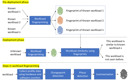
Figure 1: Flow chart: Unknown workload prediction

Figure 1 shows the overall design of our system. At a high-level, our system can be broken into two major phases: a training phase and an inference phase. The purpose of the training phase is essentially to learn the “fingerprints” of the known workloads, while the purpose of the inference phase is to detect an unknown workload by obtaining its “fingerprints” and comparing them to the fingerprints of the known workloads. The approach of comparing the fingerprints relies on the notion of workload similarity.

The steps performed by our system to obtain fingerprints of a workload are as follows: (i) executing the workload on a target system while collecting hardware and (allowed) software counters while running the workload, (ii) detecting changes in the workload phases by using Bayesian change point detection (BCPD), (iii) summarizing workload phases, and (v) generating fingerprints using summarized phases. Given a set of workloads to be used for training phase, we perform these steps on all the workloads sequentially and collect fingerprints for each of them.

V-A Telemetry Data Collection

Given a workload along with its test input, we first execute the workload and collect its profiling information by using certain hardware and software counters. In a nutshell, given a set of $n$ counters and time of $t$ seconds for which the workload is run, the output of this phase is a 2D matrix of size $n{\times}t$ (assuming that the counters were sampled for every one second). In other words, the output is a set of $n$ discrete time series. Note that the absolute values of the counters would have different magnitudes. Hence, each set of time series data is normalized using the following equation:

$$y=\frac{|x-\mu|}{\sigma}$$ (7)

where $y$, $x$, $\mu$ and $\sigma$ are a normalized value, a raw data value, the arithmetic mean and the standard deviation of time series data, respectively.

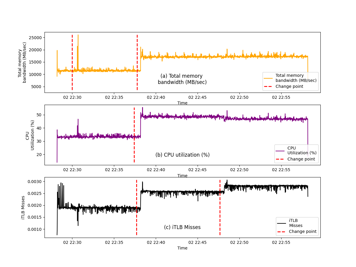
Figure 2: Phase identification using BCPD algorithm

V-B Change Point Detection

In this step, we apply the Bayesian change point detection technique (BCPD) to individual counter’s normalized time series data to locate the changepoints, which essentially represent the endpoints of phases. Intuitively, we breakdown time series for a counter into components (called phases) that are “similar” in nature (statistically). For example, Figure 2 shows the change points (in red dotted line) identified by the BCPD technique for the three different time series of total memory bandwidth, CPU utilization (%), and iTLB misses for MongoDB-ycsb workload. Note that different time series could have different number of changepoints. For instance, time series of total memory bandwidth and iTLB misses have two changepoints, while that of CPU utilization has only one changepoint.

V-C Workload Fingerprinting

The aim of this step is to generate workload-specific (in other words, unique) signature that allows us to identify that workload. We call such a unique signature a fingerprint. Concretely, we define workload fingerprint as the summary of all the phases identified in all the time series data for that workload. In this step, we use statistical measures to summarize every phase. Specifically, for each phase, we calculate the mean, median, variance, augmented Dickey-Fuller test statistics, and the distribution of the phase. If a time series has $p$ phases and $k$ is the number statics measured per phase, then the summary of that time series would be a matrix of size $p{\times}k$. However, the number of phases identified in different time series may not be same. As a result, the time series summary matrix could vary in size from counter to counter based on the number of phases ($p$). We alleviate this issue by applying zero padding to the summary matrices based on the maximum number of phases across all counters for a given workload. For example, if a workload profile data has $n$ counters, and $q$ is the highest number of phases identified across all the counters, then the workload fingerprint would be a table of size $n{\times}q{\times}k$, where $q\leq p$.

V-D Workload Similarity

This step of workload similarity is aimed at evaluating similarity of two workloads, specified using their fingerprints obtained in the previous step. Conceptually, two workloads would be similar (denoted as $\sim$) if (1) they both have same number of phases and (2) all the phases of both the workloads are mutually similar (denoted by $\approx$), meaning phase $i$ of one workload is similar to phase $i$ of the other workload. Formally, if we represent fingerprint of one workload as $(t_{1},t_{2},..,t_{m})$, where $m$ is the number of phases of that workload and $t$ is the fingerprint of a phase, and the fingerprint of another workload is $(t^{\prime}_{1},t^{\prime}_{2},..,t^{\prime}_{n})$, where $n$ is the number of phases of the second workload and $t^{\prime}$ is the fingerprint of its phase, then $(t_{1},..,t_{m})\sim(t^{\prime}_{1},..,t^{\prime}_{n}))$ if:

$$\forall i\in[1,n]\mid t_{i}\approx t^{\prime}_{i}\quad\textit{if }m=n$$

This definition of workload similarity, however, does not consider workloads having different number of phases. A simple approach to handle workloads having different number of phases could be to run them from start to end. It, nonetheless, restricts efficacy of detecting unknown workloads that are not run to completion (in other words, a small window into their execution). We consequently extend the earlier definition of workload similarity to consider this scenario. Specifically, what we need to check for is whether the workload having smaller number of phases is a portion of the workload having larger number of phases (similar to substring matching problem). Formally, we modify the above formulation as $(t_{1},..,t_{m})\sim(t^{\prime}_{1},..,t^{\prime}_{n}))$ if:

$$\begin{cases}\forall i\in[1,m],\exists j\in\mathbb{N}\mid t_{i}\approx t^{\prime}_{i+j}&\quad\text{if }m<n\\ \forall i\in[1,n],\exists j\in\mathbb{N}\mid t_{i+j}\approx t^{\prime}_{i}&\quad\text{if }m>=n\end{cases}$$

In the above equation, $j$ essentially represents an offset into the phases of the workload having larger number of phases. In other words, the workload having smaller number of phases could start at any offset within the workload having larger number of phases.

In this paper, we use Euclidean distance and dynamic time warping (DTW) technique with Manhattan distance to implement phase-level similarity function ($\approx$).

The similarity measurement between the phases of the same workload provides a threshold value to identify similar workloads. For this study, the threshold is defined as mean of phase-level similarity values $\pm$ standard deviation. If an unknown workload’s similarity measurement falls within the threshold values of a particular workload, then we can say the unknown workload is similar to that particular workload. To validate the threshold value, we randomly split the data set 70%-30% ratio to create train and validation data set. Then, we establish the threshold value from the mean and standard deviation of the same types of workloads from the training data. The accuracy of the threshold value will be validated by the validation data. For validation step, a fingerprint data from the validation data set use its phase number to identify first similar workload fingerprints from the training data and then calculate ED and DTW with identified data. The smallest value of ED and DTW will identify the most similar workload. Then, we will check the threshold value of particular workload to confirm.

VI Evaluation

VI-A Experimental Setup

To validate the proposed unknown workload prediction algorithm and ascertain its accuracy, we set up a Kubernetes cluster, known as K8S. Kubernetes is an open-source system for automating deployment, scaling and management of containerized application. As shown in Figure 3 our K8s cluster has 14 worker nodes and 1 master node.

Figure 3: System setup for data collection in Kubernets Cluster

Hardware setup

All the worker nodes and the master node were running on separate Intel Xeon processors (codenamed SkyLake), each having 2 sockets for a total of 28 cores, running at a maximum frequency of 3.9GHz and 512GB of memory. All the servers were running Ubuntu-20.04 server operating system.

Workloads

We ran a total of 6 training workloads in our experiments: mongoDB-ycsb-4.4, MySQL8, Wordpress-5MT, Bayesian inference, AI-benchmark-0.1.2 and Redis-6.0.9. These workloads cover some of the typical applications run in cloud environment. Each workload runs in a docker container.

Telemetry data collection

We used a total of 72 hardware and software counters in our experiment (some of them are shown in Table I). We execute the workloads for a total of 30 (CPU) seconds and sample the counters at every second. We believe that the initial workload execution time contains different phases such as warmup, connection setups, etc., which represent interesting set of phases for experimentation. We use PerfSpect [17] tool to collect hardware telemetry data. The PerfSpect tool, based on Linux perf collects data from the underlying hardware platform, and it has two main functions: 1) collect PMU (Performance Monitoring Unit) counters, and 2) post-processing data and generate a CSV output of performance metrics.

TABLE I: Hardware and software counters

Counter	Type
Load Instructions	Hardware
LLC Cache Misses	Hardware
L1 cache misses	Hardware
iTLB misses	Hardware
L2 cache misses	Hardware
CPU utilization	Software
Page Major Faults	Software
Total Page Cache	Software
Canonical Memory Usage	Software

VI-B Research Questions

In our evaluation, we attempt to answer following research questions:

• RQ1: How accurately can we classify known workloads as similar?

• RQ2: How does CWD perform when classifying unknown workloads?

• RQ3: What could be a threshold for classfying similar workloads?

We answer these questions by simulating 3 case studies.

We answer RQ1 in the first case study by developing an ML based supervised binary classification model that learns to classify workloads using their fingerprints. Specifically, we utilize Gradient Boosting Tree (GBT) algorithm to develop the prediction models due to the high dimensionality of the workload fingerprints We generate a labeled dataset by executing every workload 10 times (and obtaining its 10 fingerprints). For training the prediction model, we split the labeled dataset into training and test set (70%-30%), and later use the test set to evaluate the accuracy. Specifically, we split the dataset entries for every workload in 70%-30% manner; 7 entries per workload for training and 3 for evaluation.

We answer RQ2 in the second case study by training the GBT-based prediction model on the fingerprints of 4 workloads (MySQL, AI-benchmark, Redis and WordPress) and evaluating the model’s performance on 2 unknown workloads (MongoDB-ycsb and Bayesian inference).

For RQ3, we obtain distances between multiple executions of every workload from the set of 6 workloads and present those values (Section V-D).

VI-C Results and Discussion

RQ1

Table II summarizes the result for the first case study. To summarize, the accuracy of GBT-based ML model is 93%. Precision of 95% additionally indicates lower false positive rate.

TABLE II: Case Study 1: Accuracy of classifying known workloads

Name	Precision	Recall	F1 Score	Accuracy (%)
GBT	0.95	0.93	0.93	93

RQ2

For case study 2, the results are presented in Table III. The prediction model identified Bayesian inference workload as similar to AI-benchmark workload 100% of the time. We speculate that this could be because Bayesian inference workload uses Python-based framework for inference, which is also used by AI-benchmark workload as it performs neural network-based inference. In the case of mongoDB-ycsb workload, the prediction model identified it as WordPress 67% of the time and MySQL as 33% of the time. We speculate that this could be because of similar database operations performed by all three workloads. Specifically, WordPress workload runs pre-populated user blogging data with the MariaDB database, a fork of MySQL. Although, MongoDB is a NoSQL database, some of its general database operations probably stress the hardware and software counters similar to the MySQL workload and WordPress’s MariaDB operations.

TABLE III: Case Study 2: Classifying unknown workloads

	AI- benchmark	WordPress	MySQL	Redis
MongoDB-ycsb	0	67%	33%	0
Bayesian Inference	100%	0	0	0

RQ3

To answer the question about appropriate threshold values to classify similar workloads, we run every workload multiple times and calculate the distances between multiple runs of same workload. Table IV presents the mean and standard deviation of the distances for every workload. In general, DTW-based distances are larger compared ED-based distances. For both DTW and ED based distances, the largest and the smallest values are observed in Redis and AI-benchmark workloads respectively. Intuitively, the mean distances represent radius of the workload-specific circles, every point in which would represent a workload similar to that workload. So we can use these mean values as the threshold values to classify similar workloads. Figure 4 shows the visual similarity of different workload phases.

TABLE IV: Workload Similarity Measurement Using Fingerprints (DTW = dynamic time warping; ED = Euclidean distance)

Workload	DTW		ED
	Mean	Standard	Mean	Standard
		deviation		deviation
Redis	211.90	52.74	28.06	6.41
AI-benchmark	131.07	52.66	19.93	7.33
MySQL	181.94	65.53	23.51	8.45
MongoDB-ycsb	166.23	73.30	23.19	9.18
WordPress	145.25	64.47	20.21	6.94
Bayesian inference	181.60	46.69	27.93	6.32

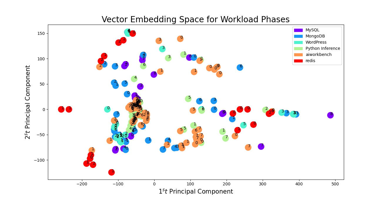
Figure 4: Figure showing different workloads phases

VII Conclusion

In this paper, we present our system named CWD that predicts workloads running in a cloud environment. It profiles and characterizes cloud workload to understand workload performance and phases. We classify cloud workloads using software and hardware performance counters to generate workload-specific fingerprints and develop formulas to measure similarity of workload phases. Our experimental evaluation performed on a set of 6 cloud workloads demonstrates high accuracy of our machine learning based model.

VIII Future work

We plan to improve this work by increasing the number of workloads run in a docker container so that we can improve workload prediction with a higher degree of confidence for our future work. We also plan to implement in production so that we can predict any unknown workload in real time.

References

- [1] Uptime Institute, “2019 Data Center Industry Survey Results” in https://uptimeinstitute.com/2019-data-center-industry-survey-results
- [2] R. Khanna, M. Ganguli, A. Narayan, A. R. and P. Gupta, “Autonomic Characterization of Workloads Using Workload Fingerprinting,” 2014 IEEE International Conference on Cloud Computing in Emerging Markets (CCEM), 2014, pp. 1-8, doi: 10.1109/CCEM.2014.7015482.
- [3] S. Jokar Jandaghi, A. Bhattacharyya and C. Amza, “Phase Annotated Learning for Apache Spark: Workload Recognition and Characterization,” 2018 IEEE International Conference on Cloud Computing Technology and Science (CloudCom), 2018, pp. 9-16, doi: 10.1109/CloudCom2018.2018.00018.
- [4] S. Elnaffar and Pat Martin, “Characterizing Computer Systems’ Workloads”: Technical report 2002-461, School of Computing, Queen’s University, Kingston
- [5] A. Bhattacharyya, C. Amza and E. de Lara, “Phase Aware Performance Modeling for Cloud Applications,” 2020 IEEE 13th International Conference on Cloud Computing (CLOUD), 2020, pp. 507-511, doi: 10.1109/CLOUD49709.2020.00075.
- [6] A. Bhattacharyya, S. Sotiriadis and C. Amza, “Online Phase Detection and Characterization of Cloud Applications,” 2017 IEEE International Conference on Cloud Computing Technology and Science (CloudCom), 2017, pp. 98-105, doi: 10.1109/CloudCom.2017.21.
- [7] T. Sherwood, S. Sair and B. Calder, “Phase tracking and prediction,” 30th Annual International Symposium on Computer Architecture, 2003. Proceedings., 2003, pp. 336-347, doi: 10.1109/ISCA.2003.1207012.
- [8] R. N. Calheiros, E. Masoumi, R. Ranjan and R. Buyya, “Workload Prediction Using ARIMA Model and Its Impact on Cloud Applications’ QoS,” in IEEE Transactions on Cloud Computing, vol. 3, no. 4, pp. 449-458, 1 Oct.-Dec. 2015, doi: 10.1109/TCC.2014.2350475.
- [9] E. Caron, F. Desprez and A. Muresan, “Forecasting for Grid and Cloud Computing On-Demand Resources Based on Pattern Matching,” 2010 IEEE Second International Conference on Cloud Computing Technology and Science, 2010, pp. 456-463, doi: 10.1109/CloudCom.2010.65.
- [10] A. Bhattacharyya, S. Sotiriadis and C. Amza, “Online Phase Detection and Characterization of Cloud Applications,” 2017 IEEE International Conference on Cloud Computing Technology and Science (CloudCom), 2017, pp. 98-105, doi: 10.1109/CloudCom.2017.21.
- [11] F. Song, Z. Guo and D. Mei, “Feature Selection Using Principal Component Analysis,” 2010 International Conference on System Science, Engineering Design and Manufacturing Informatization, 2010, pp. 27-30, doi: 10.1109/ICSEM.2010.14.
- [12] Lin Luo, M. N. S. Swamy and E. I. Plotkin, “A modified PCA algorithm for face recognition,” CCECE 2003 - Canadian Conference on Electrical and Computer Engineering. Toward a Caring and Humane Technology (Cat. No.03CH37436), 2003, pp. 57-60 vol.1, doi: 10.1109/CCECE.2003.1226343.
- [13] C. Truong, L. Oudre, N. Vayatis, “Selective review of offline change point detection methods”, University Paris 13 France https://doi.org/10.1016/j.sigpro.2019.107299
- [14] R. Malladi, G. P. Kalamangalam and B. Aazhang, “Online Bayesian change point detection algorithms for segmentation of epileptic activity,” 2013 Asilomar Conference on Signals, Systems and Computers, 2013, pp. 1833-1837, doi: 10.1109/ACSSC.2013.6810619.
- [15] A. Josang, “Generalising Bayes’ theorem in subjective logic,” 2016 IEEE International Conference on Multisensor Fusion and Integration for Intelligent Systems (MFI), 2016, pp. 462-469, doi: 10.1109/MFI.2016.7849531.
- [16] S. Sun and R. Huang, “An adaptive k-nearest neighbor algorithm,” 2010 Seventh International Conference on Fuzzy Systems and Knowledge Discovery, 2010, pp. 91-94, doi: 10.1109/FSKD.2010.5569740.
- [17] https://github.com/intel/PerfSpect
- [18] Burg, G. J. J., and C. K. I. Williams. “An evaluation of change point detection algorithms.” arXiv preprint arXiv:2003.06222 (2020).
- [19] G. T. Reddy et al., “Analysis of Dimensionality Reduction Techniques on Big Data,” in IEEE Access, vol. 8, pp. 54776-54788, 2020, doi: 10.1109/ACCESS.2020.2980942.