Malign Overfitting: Interpolation Can Provably Preclude Invariance

Abstract

Learned classifiers should often possess certain invariance properties meant to encourage fairness, robustness, or out-of-distribution generalization. However, multiple recent works empirically demonstrate that common invariance-inducing regularizers are ineffective in the over-parameterized regime, in which classifiers perfectly fit (i.e. interpolate) the training data. This suggests that the phenomenon of “benign overfitting,” in which models generalize well despite interpolating, might not favorably extend to settings in which robustness or fairness are desirable.

In this work we provide a theoretical justification for these observations. We prove that—even in the simplest of settings—any interpolating learning rule (with arbitrarily small margin) will not satisfy these invariance properties. We then propose and analyze an algorithm that—in the same setting—successfully learns a non-interpolating classifier that is provably invariant. We validate our theoretical observations on simulated data and the Waterbirds dataset.

1 Introduction

Modern machine learning applications often call for models which are not only accurate, but which are also robust to distribution shifts or satisfy fairness constraints. For example, we might wish to avoid using hospital-specific traces in X-ray images [16, 65], as they rely on spurious correlations that will not generalize to a new hospital, or we might seek “Equal Opportunity” models attaining similar error rates across protected demographic groups, e.g., in the context of loan applications [5, 22]. A developing paradigm for fulfilling such requirements is learning models that satisfy some notion of invariance [40, 41] across environments or sub-populations. For example, in the X-ray case, spurious correlations can be formalized as relationships between a feature and a label which vary across hospitals [65]. Equal Opportunity [22] can be expressed as a statistical constraint on the outputs of the model, where the false negative rate is invariant to membership in a protected group. Many techniques for learning invariant models have been proposed including penalties that encourage invariance [3, 28, 57, 60, 43, 34, 44, 25], data re-weighting [49, 63, 24], causal graph analysis [54, 55], and more [1].

While the invariance paradigm holds promise for delivering robust and fair models, many current invariance-inducing methods often fail to improve over naive approaches. This is especially noticeable when these methods are used with overparameterized deep models capable of interpolating, i.e., perfectly fitting the training data [20, 18, 21, 68, 36, 58, 12]. Existing theory explains why overparameterization hurts invariance for standard interpolating learning rules, such as empirical risk minimization and max-margin classification [50, 37, 15], and also why reweighting and some types of distributionally robust optimization face challenges when used with overparameterized models [6, 49]. In contrast, training overparameterized models to interpolate the training data typically results in good in-distribution generalization, and such “benign overfitting” [26, 63] is considered a key characteristic of modern deep learning [8, 62, 52]. Consequently, a number of works attempt to extend benign overfitting to robust or fair generalization by designing new interpolating learning rules [7, 26, 63, 33].

In this paper, we demonstrate that such attempts face a fundamental obstacle, because all interpolating learning rules (and not just maximum-margin classifiers) fail to produce invariant models in certain high-dimensional settings where invariant learning (without interpolation) is possible. This does not occur because there are no invariant models that separate the data, but because interpolating learning rules cannot find them. In other words, beyond identically-distributed test sets, overfitting is no longer benign. More concretely, we consider linear classification in a basic overparameterized Gaussian mixture model with invariant “core” features as well as environment-dependent “spurious” features, similar to models used in previous work to gain insight into robustness and invariance [51, 45, 50]. We show that any learning rule producing a classifier that separates the data with non-zero margin must necessarily rely on the spurious features in the data, and therefore cannot be invariant. Moreover, in the same setting we analyze a simple two-stage algorithm that can find accurate and nearly invariant linear classifiers, i.e., with almost no dependence on the spurious feature.

Thus, we establish a separation between the level of invariance attained by interpolating and non-interpolating learning rules. We believe that learning rules which fail in the simple over-parameterized linear classification setting we consider are not likely to succeed in more complicated, real-world settings. Therefore, our analysis provides useful guidance for future research into robust and fair machine learning models, as well as theoretical support for the recent success of non-interpolating robust learning schemes [46, 58, 27, 36, 29, 67, 24, 10].

Paper organization. The next section formally states our full result (Theorem 1). In Section 3 we outline the arguments leading to the negative part of Theorem 1, i.e., the failure of interpolating classifiers to be invariant in our model. In Section 4 we establish the positive part Theorem 1, by providing and analyzing a non-interpolating algorithm that, in our model, achieves low robust error. We validate our theoretical findings with simulations and experiments on the Waterbirds dataset in Section 5, and conclude with a discussion of additional related results and directions for future research in Section 6.

2 Statement of Main Result

2.1 Preliminaries

Data model.

Our analysis focuses on learning linear models over covariates ${\mathbf{x}}$ distributed as a mixture of two Gaussian distributions corresponding to the label $y$.

Definition 1.

An environment is a distribution parameterized by $({\bm{\mu}}_{c},{\bm{\mu}}_{s},d,\sigma,\theta)$ where $\theta\in{[-1,1]}$ and ${\bm{\mu}}_{c},{\bm{\mu}}_{s}\in{\mathbb{R}^{d}}$ satisfy ${\bm{\mu}}_{c}\perp{\bm{\mu}}_{s}$ and with samples generated according to:

$${\mathbb{P}}_{\theta}(y)=\textnormal{Unif}{\{-1,1\}},\quad{\mathbb{P}}_{\theta}({\mathbf{x}}|y)=\mathcal{N}(y{\bm{\mu}}_{c}+y\theta{\bm{\mu}}_{s},\sigma^{2}I).$$ (1)

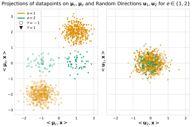
Figure 3: Example of datasets sampled from two training envrionments, where we set $\theta_{1}=1,\theta_{2}=0,$ $N_{1}=800,N_{2}=100,r_{s}=2,r_{c}=1$. Left and right plots show projections of training points on ${\bm{\mu}}_{c},{\bm{\mu}}_{s}\in{\mathbb{R}^{d}}$, and on ${\mathbf{u}}_{1},{\mathbf{u}}_{2}$ drawn uniformly from the $d$-dimensional unit sphere, respectively. As we increase $d$ there are many hyperplanes ${\mathbf{w}}\in{\mathbb{R}^{d}}$ that separate the data, for some $\langle{\mathbf{w}},\mu_{c}\rangle$ is much higher than $\langle{\mathbf{w}},\mu_{s}\rangle$ (i.e. their predictions are invariant) and for some the opposite may hold. We ask whether interpolating learning rules can find the former.

Our goal is to find a (linear) classifier that predicts $y$ from ${\mathbf{x}}$ and is robust to the value of $\theta$ (we discuss the specific robustness metric below). To do so, the classifier will need to have significant inner product with the “core” signal component ${\bm{\mu}}_{c}$ and be approximately orthogonal to the “spurious” component ${\bm{\mu}}_{s}$. We focus on learning problems where we are given access to samples from two environments that share all their parameters other than $\theta$, as we define next. We illustrate our setting with Figure 3 in Appendix A.

Definition 2 (Linear Two Environment Problem).

In a Linear Two Environment Problem we have datasets $S_{1}=\{{\mathbf{x}}_{i}^{(1)},y_{i}^{(1)}\}_{i=1}^{N_{1}}$ and $S_{2}=\{{\mathbf{x}}_{i}^{(2)},y_{i}^{(2)}\}_{i=1}^{N_{2}}$ of sizes $N_{1},N_{2}$ drawn from ${\mathbb{P}}_{\theta_{1}}$ and ${\mathbb{P}}_{\theta_{2}}$ respectively. A learning algorithm is a (possibly randomized) mapping from the tuple $(S_{1},S_{2})$ to a linear classifier ${\mathbf{w}}\in{\mathbb{R}^{d}}$. We let $S=\{{\mathbf{x}}_{i},y_{i}\}_{i=1}^{N}$ denote that dataset pooled from $S_{1}$ and $S_{2}$ where $N=N_{1}+N_{2}$. Finally we let $r_{c}\coloneqq\|{\bm{\mu}}_{c}\|$ and $r_{s}\coloneqq\|{\bm{\mu}}_{s}\|$.

We study settings where $\theta_{1},\theta_{2}$ are fixed and $d$ is large compared to $N$, i.e. the overparameterized regime. We refer to the two distributions ${\mathbb{P}}_{\theta_{e}}$ for $e\in{\{1,2\}}$ as “training environments”, following [40, 3]. In the context of Out-of-Distribution (OOD) generalization, environments correspond to different experimental conditions, e.g., collection of medical data in two hospitals. In a fairness context, we may think of these distributions as subpopulations (e.g., demographic groups).While these are different applications that require specialized methods, the underlying formalism of solutions is often similar [see, e.g., 14, Table 1], where we wish to learn a classifier that in one way or another is invariant to the environment variable.

Robust performance metric.

An advantage of the simple model defined above is that many of the common invariance criteria all boil down to the same mathematical constraint: learning a classifier that is orthogonal to ${\bm{\mu}}_{s}$, which induces a spurious correlation between the environment and the label. These include Equalized Odds [22], conditional distribution matching [31], calibration on multiple subsets of the data [23, 60], Risk Extrapolation [28] and CVaR fairness [64].

In terms of predictive accuracy, the goal of learning a linear model that aligns with ${\bm{\mu}}_{c}$ (the invariant part of the data generating process for the label) and is orthogonal to ${\bm{\mu}}_{s}$ coincides with providing guarantees on the robust error, i.e. the error when data is generated with values of $\theta$ that are different from the $\theta_{1},\theta_{2}$ used to generate training data.

Definition 3 (Robust error).

The robust error of a linear classifier ${\mathbf{w}}\in\mathbb{R}^{d}$ is:

$$\max_{\theta\in{[-1,1]}}{\epsilon_{\theta}({\mathbf{w}})},\ \text{where}\ \epsilon_{\theta}({\mathbf{w}}):={\mathbb{E}_{\begin{subarray}{c}{\mathbf{x}},y\sim{\mathbb{P}}_{\theta}\end{subarray}}\left[\mathrm{sign}(\langle{\mathbf{w}},{\mathbf{x}}\rangle)\neq y\right]}.$$ (2)

Normalized margin.

We study is whether algorithms that perfectly fit (i.e. interpolate) their training data can learn models with low robust error. Ideally, we would like to give a result on all classifiers that attain training error zero in terms of the $0$-$1$ loss. However, the inherent discontinuity of this loss would make any such statement sensitive to instabilities and pathologies. For instance, if we do not limit the capacity of our models, we can turn any classifier into an interpolating one by adding “special cases” for the training points, yet intuitively this is not the type of interpolation that we would like to study. To avoid such issues, we replace the 0-1 loss with a common continuous surrogate, the normalize margin, and require it to be strictly positive.

Definition 4 (Normalized margin).

Let $\gamma>0$, we say a classifier ${\mathbf{w}}\in{\mathbb{R}^{d}}$ separates the set $S=\{{\mathbf{x}}_{i},y_{i}\}_{i=1}^{N}$ with normalized margin $\gamma$ if for every $({\bm{x}},y)\in S$

$$\frac{y_{i}\langle{\mathbf{w}},{\mathbf{x}}_{i}\rangle}{\|{\mathbf{w}}\|}>\gamma\sqrt{\sigma^{2}d}.$$

The $\sqrt{\sigma^{2}d}$ scaling of $\gamma$ is roughly proportional to $\|{\mathbf{x}}\|$ under our data model in Equation (1), and keeps the value of $\gamma$ comparable across growing values of $d$.

2.2 Main Result

Equipped with the necessary definitions, we now state and discuss our main result.

Theorem 1.

For any sample sizes $N_{1},N_{2}>65$, margin lower bound $\gamma\leq\frac{1}{4\sqrt{N}}$, target robust error $\epsilon>0$, and coefficients $\theta_{1}=1$, $\theta_{2}>-\frac{N_{1}\gamma}{\sqrt{288N_{2}}}$, there exist parameters $r_{c},r_{s}>0$, $d>N$, and $\sigma>0$ such that the following holds for the Linear Two Environment Problem (Definition 2) with these parameters.

1. Invariance is attainable. Algorithm 1 maps $(S_{1},S_{2})$ to a linear classifier ${{\mathbf{w}}}$ such that with probability at least $\frac{99}{100}$ (over the draw $S$), the robust error of ${\mathbf{w}}$ is less than $\epsilon$.

2. Interpolation is attainable. With probability at least $\frac{99}{100}$, the estimator ${\mathbf{w}}_{\mathrm{mean}}=N^{-1}\sum_{i\in[N]}{y_{i}{\mathbf{x}}_{i}}$ separates $S$ with normalized margin (Definition 4) greater than $\frac{1}{4\sqrt{N}}$.

3. Interpolation precludes invariance. Given ${\bm{\mu}}_{c}$ uniformly distributed on the sphere of radius $r_{c}$ and ${\bm{\mu}}_{s}$ uniformly distributed on a sphere of radius $r_{s}$ in the subspace orthogonal to ${\bm{\mu}}_{c}$, let ${\mathbf{w}}$ be any classifier learned from $(S_{1},S_{2})$ as per Definition 2. If ${{\mathbf{w}}}$ separates $S$ with normalized margin $\gamma$, then with probability at least $\frac{99}{100}$ (over the draw of ${\bm{\mu}}_{c},{\bm{\mu}}_{s}$, and the sample), the robust error of ${\mathbf{w}}$ is at least $\frac{1}{2}$.

Theorem 1 shows that if a learning algorithm for overparameterized linear classifiers always separates its training data, then there exist natural settings for which the algorithm completely fails to learn a robust classifier, and will therefore fail on multiple other invariance and fairness objectives. Furthermore, in the same setting this failure is avoidable, as there exists an algorithm (that necessarily does not always separate its training data) which successfully learns an invariant classifier. This result has deep implications for theoreticians attempting to prove finite-sample invariant learning guarantees: it shows that—in the fundamental setting of linear classification—no interpolating algorithm can have guarantees as strong as non-interpolating algorithms such as Algorithm 1.

Importantly, Theorem 1 requires interpolating invariant classifiers to exist—and shows that these classifiers are information-theoretically impossible to learn. In particular, the first part of the theorem implies that the Bayes optimal invariant classifier ${\bm{w}}={\bm{\mu}}_{c}$ has robust test error at most $\epsilon$. Therefore, for all $\epsilon<\frac{1}{100N}$ we have that ${\bm{\mu}}_{c}$ interpolates $S$ with probability $>\frac{99}{100}$. Furthermore, a short calculation (see Section C.1) shows that (for $r_{c}$, $r_{s}$, $d$ and $\sigma$ satisfying Theorem 1) the normalized margin of ${\bm{\mu}}_{c}$ is $\Omega(({N+\sqrt{N_{2}}/\gamma})^{-\frac{1}{2}})$. However, we prove that—due to the high-dimensional nature of the problem—no algorithm can use $(S_{1},S_{2})$ to reliably distinguish the invariant interpolator from other interpolators with similar or larger margin. This learnability barrier strongly leverages our random choice of ${\bm{\mu}}_{c}$, ${\bm{\mu}}_{s}$, without which the (fixed) vector ${\bm{\mu}}_{c}$ would be a valid learning output.

We establish Theorem 1 with three propositions, each corresponding to an enumerated claim in the theorem: (1) Proposition 2 (in §4) establishes that invariance is attainable, (2) Proposition 3 (Appendix C) establishes that interpolation is attainable, and (3) Proposition 1 (in §3) establishes that interpolation precludes invariance. We choose to begin with the latter proposition since it is the main conceptual and technical contribution of our paper. Conversely, Proposition 3 is an easy byproduct of the developments leading up to Proposition 1, and we defer it to the appendix.

With Propositions 1, 2 and 3 in hand, the proof of Theorem 1 simply consists of choosing the free parameters in Theorem 1 ($r_{c},r_{s},d$ and $\sigma$) based on these propositions such that all the claims in the theorem hold simultaneously. For convenience we take $\sigma^{2}=1/d$. Then (ignoring constant factors) we pick $r_{s}^{2}\propto\frac{1}{N}$ and $r_{c}^{2}\propto r_{s}^{2}/(1+\frac{\sqrt{N_{2}}}{N_{1}\gamma})$ in order to satisfy requirements in Propositions 1 and 3. Finally, we take $d$ to be sufficiently large so as to satisfy the remaining requirements, resulting in $d\propto\max\left\{N^{2},\frac{N}{\gamma^{2}N_{1}^{2}r_{c}^{2}},\frac{(Q^{-1}(\epsilon))^{2}}{N_{\min}r_{c}^{4}},\frac{1}{N_{\min}^{2}r_{c}^{4}}\right\}$, where $N_{\min}=\min\{N_{1},N_{2}\}$ and $Q$ is the Gaussian tail function (see Appendix E for the full proof).

We conclude this section with remarks on the range of parameters under which Theorem 1 holds. The impossibility results in Theorem 1 are strongest when $N_{2}$ is smaller than $N_{1}^{2}\gamma^{2}$. In particular, when $N_{2}\leq N_{1}^{2}\gamma^{2}/288$, our result holds for all $\theta_{2}\in[-1,1]$ and moreover the core and spurious signal strengths $r_{c}$ and $r_{s}$ can be chosen to be of the same order. The ratio $N_{2}/(N_{1}^{2}\gamma^{2})$ is small either when one group is under-represented (i.e., $N_{2}\ll N_{1}$) or when considering large margin classifiers (i.e., $\gamma$ of the order $1/\sqrt{N}$). Moreover, unlike prior work on barriers to robustness [e.g., 50, 37], our result continue to hold even for balanced data and arbitrarily low margin, provided $\theta_{2}$ is close to $0$ and the core signal is sufficiently weaker than the spurious signal. Notably, the normalized margin $\gamma$ can be arbitrarily small while the maximum achievable margin is always at least of the order of $\frac{1}{\sqrt{N}}$. Therefore, we believe that Theorem 1 essentially precludes any interpolating learning rule from being consistently invariant.

3 Interpolating Models Cannot Be Invariant

In this section we prove the third claim in Theorem 1: for essentially any nonzero value of the normalized margin $\gamma$, there are instances of the Linear Two Environment Problem (Definition 2) where with high probability, learning algorithms that return linear classifiers attaining normalized margin at least $\gamma$ must incur a large robust error. The following proposition formalizes the claim; we sketch the proof below and provide a full derivation in Section B.3.

Proposition 1.

For $\sigma=1/\sqrt{d}$, $\theta_{1}=1$, there are universal constants $c_{r}\in(0,1)$ and $C_{d},C_{r}\in(1,\infty)$, such that, for any target normalized $\gamma$, $\theta_{2}>-N_{1}\gamma/\sqrt{288N_{2}}$, and failure probability $\delta\in(0,1)$, if

$$\max\{r_{s}^{2},r_{c}^{2}\}\leq\frac{c_{r}}{N}~{}~{},~{}~{}\frac{r_{s}^{2}}{r_{c}^{2}}\geq C_{r}\left(1+\frac{\sqrt{N_{2}}}{N_{1}\gamma}\right)~{}~{}\mbox{ and}~{}~{}$$ (3)

$$d\geq C_{d}\frac{N}{\gamma^{2}N_{1}^{2}r_{c}^{2}}\log\frac{1}{\delta},$$ (4)

then with probability at least $1-\delta$ over the drawing of ${\bm{\mu}}_{c},{\bm{\mu}}_{s}$ and $(S_{1},S_{2})$ as described in Theorem  1, any $\hat{{\mathbf{w}}}\in{\mathbb{R}^{d}}$ that is a measurable function of $(S_{1},S_{2})$ and separates the data with normalized margin larger than $\gamma$ has robust error at least $0.5$.

Proof sketch.

We begin by noting that for any fixed $\theta$, the error of a linear classifier ${\mathbf{w}}$ is

$$\epsilon_{\theta}({\mathbf{w}})=Q\left(\frac{\langle{\mathbf{w}},{\bm{\mu}}_{c}\rangle+\theta\langle{\mathbf{w}},{\bm{\mu}}_{s}\rangle}{\sigma\|{\mathbf{w}}\|}\right)=Q\left(\frac{\langle{\mathbf{w}},{\bm{\mu}}_{c}\rangle}{\sigma\|{\mathbf{w}}\|}\left(1+\theta\frac{\langle{\mathbf{w}},{\bm{\mu}}_{s}\rangle}{\langle{\mathbf{w}},{\bm{\mu}}_{c}\rangle}\right)\right),$$ (5)

where $Q(t)\coloneqq\mathbb{P}(\mathcal{N}(0;1)>t)$ is the Gaussian tail function. Consequently, when $\langle{\mathbf{w}},{\bm{\mu}}_{s}\rangle/\langle{\mathbf{w}},{\bm{\mu}}_{c}\rangle\geq 1$ it is easy to see that $\epsilon_{\theta}({\mathbf{w}})=1/2$ for some $\theta\in[-1,1]$ and therefore the robust error is at least $\frac{1}{2}$; we prove that $\langle{\mathbf{w}},{\bm{\mu}}_{s}\rangle/\langle{\mathbf{w}},{\bm{\mu}}_{c}\rangle\geq 1$ indeed holds with high probability under the proposition’s assumptions. Our proof has two key parts: (a) restricting the set of classifiers to the linear span of the data and (b) lower bounding the minimum value of $\langle{\mathbf{w}},{\bm{\mu}}_{s}\rangle/\langle{\mathbf{w}},{\bm{\mu}}_{c}\rangle$ for classifier in that linear span.

For the first part of the proof we use the spherical distribution of ${\bm{\mu}}_{c}$ and ${\bm{\mu}}_{s}$ and concentration of measure to show that (with high probability) any component of ${\mathbf{w}}$ chosen outside the linear span of $\{{\mathbf{x}}_{i}\}_{i\in[N]}$ will have negligible effect on the predictions of the classifier. To explain this fact, let ${\bm{P}}_{\perp}$ denote the projection operator to the orthogonal complement of the data, so that ${\bm{P}}_{\perp}{\mathbf{w}}$ is the component of ${\mathbf{w}}$ orthogonal to the data and $\langle{\bm{P}}_{\perp}{\mathbf{w}},{\bm{\mu}}_{c}\rangle=\left\langle{\mathbf{w}},\frac{{\bm{P}}_{\perp}{\bm{\mu}}_{c}}{\|{\bm{P}}_{\perp}{\bm{\mu}}_{c}\|}\right\rangle\|{\bm{P}}_{\perp}{\bm{\mu}}_{c}\|$. Conditional on $(S_{1},S_{2})$ and the learning rule’s random seed, the vector ${\bm{P}}_{\perp}{\bm{\mu}}_{c}/\|{\bm{P}}_{\perp}{\bm{\mu}}_{c}\|$ is uniformly distributed on a unit sphere of dimension $d-N$ while the vector ${\mathbf{w}}$ is deterministic. Assuming without loss of generality that $\|{\mathbf{w}}\|=1$, concentration of measure on the sphere implies that $|\langle{\mathbf{w}},\frac{{\bm{P}}_{\perp}{\bm{\mu}}_{c}}{\|{\bm{P}}_{\perp}{\bm{\mu}}_{c}\|}\rangle|$ is (with high probability) bounded by roughly $1/\sqrt{d}$, and therefore $|\langle{\bm{P}}_{\perp}{\mathbf{w}},{\bm{\mu}}_{c}\rangle|$ is roughly of the order $r_{c}/\sqrt{d}$. For sufficiently large $d$ (as required by the proposition), this inner product would be negligible, meaning that $\langle{\mathbf{w}},{\bm{\mu}}_{c}\rangle$ is roughly the same as $\langle(I-{\bm{P}}_{\perp}){\mathbf{w}},{\bm{\mu}}_{c}\rangle$, and $(I-{\bm{P}}_{\perp}){\mathbf{w}}$ is in the span of the data. The same argument applies to ${\bm{\mu}}_{s}$ as well.

In the second part of the proof, we consider classifiers of the form ${\mathbf{w}}=\sum_{i\in[N]}\beta_{i}y_{i}{\mathbf{x}}_{i}$ (which parameterizes the linear span of the data) and minimize $\langle{\mathbf{w}},{\bm{\mu}}_{s}\rangle/\langle{\mathbf{w}},{\bm{\mu}}_{c}\rangle$ over $\beta\in\mathbb{R}^{N}$ subject to the constraint that ${\mathbf{w}}$ has normalize margin of at least $\gamma$. To do so, we first use concentration of measure to argue that it is sufficient to lower bound $\sum_{i\in[N_{1}]}\beta_{i}$ subject to the margin constraint and $\|{\mathbf{w}}\|^{2}\leq 1$, which is convex in $\beta$—we obtain this lower bound by analyzing the Lagrange dual of the problem of minimizing $\sum_{i\in[N_{1}]}\beta_{i}$ subject to these constraints.

Overall, we show a high-probability lower bound on $\frac{\langle{\mathbf{w}},{\bm{\mu}}_{s}\rangle}{\langle{\mathbf{w}},{\bm{\mu}}_{c}\rangle}$ that (for sufficiently high dimensions) scales roughly as $\frac{r_{s}^{2}N_{1}\gamma}{r_{c}^{2}\sqrt{N_{2}}}$. For parameters satisfying Equation (3) we thus obtain $\frac{\langle{\mathbf{w}},{\bm{\mu}}_{s}\rangle}{\langle{\mathbf{w}},{\bm{\mu}}_{c}\rangle}\geq 1$, completing the proof. ∎

Implication for invariance-inducing algorithms.

Our proof implies that any interpolating algorithm should fail at learning invariant classifiers. This alone does not necessarily imply that specific algorithms proposed in the literature for learning invariant classifiers fail, as they may not be interpolating. Yet our simulations in Section 5 show that several popular algorithms proposed for eliminating spurious features are indeed interpolating in the overparameterized regime. We also give a formal statement in Appendix G regarding the IRMv1 penalty [3], showing that it is biased toward large margins when applied to separable datasets. Our results may seem discouraging for the development of invariance-inducing techniques using overparameterized models. It is natural to ask what type of methods can provably learn such models, which is the topic of the next section.

4 A Provably Invariant Overparameterized Estimator

We now turn to propose and analyze an algorithm (Algorithm 1) that provably learns an overparametrized linear model with good robust accuracy in our setup. Our approach is a two-staged learning procedure that is conceptually similar to some recently proposed methods [46, 58, 27, 36, 29, 67]. In Section 5 we validate our algorithm on simulations and on the Waterbirds dataset [49], but we leave a thorough empirical evaluation of the techniques described here to future work.

Let us describe the operation of Algorithm 1. First, we evenly split the data from each environment into the sets $S^{\mathrm{train}}_{e},S^{\mathrm{post}}_{e}$, for $e\in\{1,2\}$. The two stages of the algorithm operate on different splits of the data as follows.

1. “Training” stage: We use $\{S^{\mathrm{train}}_{e}\}$ to fit overparameterized, interpolating classifiers $\{{\mathbf{w}}_{e}\}$ separately for each environment $e\in{\{1,2\}}$.

2. “Post-processing” stage: We use the second portion of the data $\left(S^{\mathrm{post}}_{1},S^{\mathrm{post}}_{2}\right)$ to learn an invariant linear classifier over a new representation, which concatenates the outputs of the classifiers in the first stage. In particular, we learn this classifier by maximizing a score (i.e., minimizing an empirical loss), subject to an empirical version of an invariance constraint. For generality we denote this constraint by membership in some set of functions $\mathcal{F}(S^{\mathrm{post}}_{1},S^{\mathrm{post}}_{2})$.

Crucially, the invariance penalty is only used in the second stage, in which we are no longer in the overparamterized regime since we are only fitting a two-dimensional classifier. In this way we overcome the negative result from Section 3.

While our approach is general and can handle a variety of invariance notions (we discuss some of them in Appendix F), we analyze the algorithm under the Equal Opportunity (EOpp) criterion [22]. Namely, for a model $f:\mathbb{R}^{d}\rightarrow\mathbb{R}$ we write:

$$\mathcal{F}(S_{1}^{\mathrm{fine}},S_{2}^{\mathrm{fine}})=\big{\{}f:\hat{T}_{1}(f) =\hat{T}_{2}(f)\big{\}},\quad\text{where}\ \hat{T}_{e}(f):=\frac{4}{N_{e}}\sum_{({\mathbf{x}},y)\in{S_{e}^{\mathrm{fine}}}:y=1}{f({\mathbf{x}})}.$$

This is the empirical version of the constraint $\mathbb{E}_{{\mathbb{P}}_{\theta_{1}}}\left[f(x)|y=1\right]=\mathbb{E}_{{\mathbb{P}}_{\theta_{2}}}\left[f(x)|y=1\right]$. From a fairness perspective (e.g., thinking of a loan application), this constraint ensures that the “qualified” members (i.e., those with $y=1$) of each group receive similar predictions, on average over the entire group.

Algorithm 1 Two Phase Learning of Overparameterized Invariant Classifiers

Datasets $(S_{1},S_{2})$ and an invariance constraint function family $\mathcal{F}(\cdot,\cdot)$

A classifier $f_{{\mathbf{v}}}({\mathbf{x}})$

Draw subsets of data without replacement $S^{\mathrm{train}}_{e}\subset S_{e}$ for $e\in{\{1,2\}}$ where $\left|S^{\mathrm{train}}_{e}\right|=N_{e}/2$

Stage 1: Calculate ${\mathbf{w}}_{e}=2N_{e}^{-1}\sum_{({\mathbf{x}},y)\in{S^{\mathrm{train}}_{e}}}{y{\mathbf{x}}}$ for each $e\in{\{1,2\}}$

Define $S_{e}^{\mathrm{fine}}=S_{e}\setminus S_{e}^{\mathrm{trn}}$ for $e\in{\{1,2\}}$ and $S^{\mathrm{post}}=S_{1}^{\mathrm{fine}}\cup S_{2}^{\mathrm{fine}}$

Stage 2: Return $f_{{\mathbf{v}}}({\mathbf{x}})=\langle v_{1}\cdot{\mathbf{w}}_{1}+v_{2}\cdot{\mathbf{w}}_{2},{\mathbf{x}}\rangle$ that solves

$$\operatorname*{maximize}\sum_{({\mathbf{x}},y)\in{S^{\mathrm{post}}}}{yf_{{\mathbf{v}}}({\mathbf{x}})}\quad\text{subject to}\quad{\|{\mathbf{v}}\|_{\infty}=1}\quad\text{and}\quad f_{\mathbf{v}}\in{\mathcal{F}(S_{1}^{\mathrm{fine}},S_{2}^{\mathrm{fine}})}$$

We now turn to providing conditions under which Algorithm 1 successfully learns an invariant predictor. The full proof for the following proposition can be found in section D.1 of the appendix. While we do not consider the following proposition very surprising, the fact that it gives a finite sample learning guarantee means it does not directly follow from existing work (discussed in §6 below) that mostly assume inifinite sample size.

Proposition 2.

Consider the Linear Two Environment Problem (Definition 2), and further suppose that $|\theta_{1}-\theta_{2}|>0.1$. There exist universal constants $C_{p},C_{c},C_{s}\in(1,\infty)$ such that the following holds for every target robust error $\epsilon>0$ and failure probability $\delta\in(0,1)$. If $N_{\min}\coloneqq\min\{N_{1},N_{2}\}\geq C_{p}\log(4/\delta)$ for some $C_{p}\in(1,\infty),$

$$r_{s}^{2}\geq\ C_{s}\sqrt{\log\frac{68}{\delta}}\frac{\sigma^{2}\sqrt{d}}{N_{\min}},~{}r_{c}^{2}\geq\ C_{c}\sigma^{2}\sqrt{\log\frac{68}{\delta}}\max\left\{Q^{-1}(\epsilon)\sqrt{\frac{d}{N_{\min}}},\frac{\sqrt{d}}{N_{\min}},\frac{r_{s}^{2}}{N_{\min}r_{c}^{2}}\right\},$$ (6)

$$\mbox{and}~{}~{}d\geq\log\frac{68}{\delta}$$ (7)

then, with probability at least $1-\delta$ over the draw of the training data and the split of the data between the two stages of learning, the robust error of the model returned by Algorithm 1 does not exceed $\epsilon$.

Proof sketch.

Writing down the error of $f_{{\mathbf{v}}}=v_{1}\cdot{\mathbf{w}}_{1}+v_{2}\cdot{\mathbf{w}}_{2}$ under $\mathbb{P}_{\theta}$, it can be shown that to obtain the desired bound on the robust error of the classifier returned by Algorithm 1, we must upper bound the ratio

$$\frac{(v_{1}^{\star}\theta_{1}+v_{2}^{\star}\theta_{2})\|{\bm{\mu}}_{s}\|^{2}+\langle{\bm{\mu}}_{s},v_{1}^{\star}\bar{{\mathbf{n}}}_{1}+v_{2}^{\star}\bar{{\mathbf{n}}}_{2}\rangle}{(v_{1}^{\star}+v_{2}^{\star})\|{\bm{\mu}}_{c}\|^{2}+\langle{\bm{\mu}}_{c},v_{1}^{\star}\bar{{\mathbf{n}}}_{1}+v_{2}^{\star}\bar{{\mathbf{n}}}_{2}\rangle},$$

when $\bar{{\mathbf{n}}}_{e}$ is the mean of Gaussian noise vectors, and $v_{1}^{\star}$ and $v_{2}^{\star}$ are the solutions to the optimization problem in Stage 2 of Algorithm 1. The terms involving inner-products with the noise terms are zero-mean and can be bounded using standard Gaussian concentration arguments. Therefore, the main effort of the proof is upper bounding

$$\frac{v_{1}^{\star}\theta_{1}+v_{2}^{\star}\theta_{2}}{v_{1}^{\star}+v_{2}^{\star}}\cdot\frac{\|{\bm{\mu}}_{s}\|^{2}}{\|{\bm{\mu}}_{c}\|^{2}}.$$

To this end, we leverage the EOpp constraint. The population version of this constraint (corresponding to infinite $N_{1}$ and $N_{2}$) implies that $v_{1}^{\star}\theta_{1}+v_{2}^{\star}\theta_{2}=0$. For finite sample sizes, we use standard Gaussian concentration and the Hanson-Wright inequality to show that the empirical EOpp constraint implies that $|v_{1}^{\star}\theta_{1}+v_{2}^{\star}\theta_{2}|$ goes to zero as the sample sizes increase. Furthermore, we argue that $\left|v_{1}^{\star}+v_{2}^{\star}\right|\geq|\theta_{1}-\theta_{2}|/2$, implying that—for appropriately large sample sizes—the above ratio indeed goes to zero. ∎

5 Empirical Validation

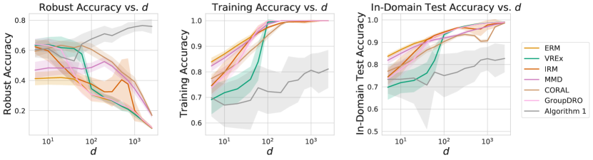
Figure 1: Numerical validation of our theoretical claims. Invariance inducing methods improve robust accuracy compared to ERM in low values of $d$, but their ability to do so is diminished as $d$ grows (top plot) and they enter the interpolation regime, as seen on the bottom plot for $d>10^{2}$. Algorithm 1 learns robust predictors as $d$ grows and does not interpolate.

The empirical observations that motivated this work can be found across the literature. We therefore focus our simulations on validating the theoretical results in our simplified model. We also evaluate Algorithm 1 on the Waterbirds dataset, where the goal is not to show state-of-the-art results, but rather to observe whether our claims hold beyond the Linear Two Environment Problem.

5.1 Simluations

Setup.

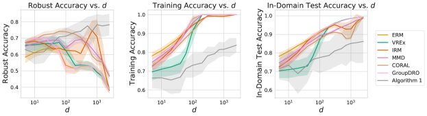
Figure 4: Results of the simulation described in Section 5.1 with $\theta_{2}=-\frac{1}{2}$ (all other parameters are kept at the same value as in Section 5.1)

We generate data as described in Theorem  1 with two environments where $\theta_{1}=1,\theta_{2}=0$ (see Figure 4 in the appendix for results of the same simulation when $\theta=-\frac{1}{2}$). We further fix $r_{c}=1$ and $r_{c}=2$, while $N_{1}=800$ and $N_{2}=100$. We then take growing values of $d$, while adjusting $\sigma$ so that $\left(r_{c}/\sigma\right)^{2}\propto\sqrt{d/N}$. For each value of $d$ we train linear models with IRMv1 [3], VREx [28], MMD [31], CORAL [56], GroupDRO [49], implemented in the Domainbed package [20]. We also train a classifier with the logistic loss to minimize empirical error (ERM), and apply Algorithm 1 where the “post-processing” stage trains a linear model over the two-dimensional representation using the VREx penalty to induce invariance. We repeat this for $15$ random seeds for drawing ${\bm{\mu}}_{c},{\bm{\mu}}_{s}$ and the training set.

Evaluation and results.

We compare the robust accuracy and the train set accuracy of the learned classifiers as $d$ grows. First, we observe that all methods except for Algorithm 1 attain perfect accuracy for large enough $d$, i.e., they interpolate. We further note that while invariance-inducing methods give a desirable effect in low dimensions (the non-interpolating regime)—significantly improving the robust error over ERM—they become aligned with ERM in terms of robust accuracy as they go deeper into the interpolation regime (indeed, IRM essentially coincides with ERM for larger $d$). This is an expected outcome considering our findings in section 3, as we set here $N_{1}$ to be considerably larger than $N_{2}$.

5.2 Waterbirds Dataset

We evaluate Algorithm 1 on the Waterbirds dataset [49], which has been previously used to evaluate the fairness and robustness of deep learning models.

Setup.

Waterbirds is a synthetically created dataset containing images of water- and land-birds overlaid on water and land background. Most of the waterbirds (landbirds) appear in water (land) backgrounds, with a smaller minority of waterbirds (landbirds) appearing on land (water) backgrounds. We set up the problem following previous work [50, 58], where a logistic regression model is trained over random features extract from a fixed pre-trained ResNet-18. Please see Appendix H for details.

Fairness.

We use the image background type (water or land) as the sensitive feature, denoted $A$, and consider the fairness desiderata of Equal Opportunity [22], i.e., the false negative rate (FNR) should be similar for both groups. Towards this, we use the MinDiff penalty term [42]. The

Evaluation.

We compare the following methods: (1) Baseline: Learning a linear classifier ${\mathbf{w}}$ by minimizing $\mathcal{L}_{p}+\lambda\cdot\mathcal{L}_{M}$, where $\mathcal{L}_{p}$ is the standard binary cross entropy loss and $\mathcal{L}_{M}$ is the MinDiff penalty; (2) Algorithm 1: In the first stage, we learn group-specific linear classifiers ${\mathbf{w}}_{0},{\mathbf{w}}_{1}$ by minimizing $\mathcal{L}_{p}$ on the examples from $A=0$ and $A=1$, respectively. In the second stage we learn ${\bm{v}}\in\mathbb{R}^{2}$ by minimizing $\mathcal{L}_{p}+\lambda\cdot\mathcal{L}_{M}$ on examples the entire dataset, where the new representation of the data is $\tilde{X}=[\langle w_{1},X\rangle,\langle w_{2},X\rangle]\in\mathbb{R}^{2}$.

Results.

Our main objective is to understand the effect of the fairness penalty. Toward this, for each method we compare both the test error and the test FNR gap when using either $\lambda=0$ (no regularization) or $\lambda=5$. The results are summarized in Figure 2. We can see that for the baseline approach, the fairness penalty successfully reduces the FNR gap when the classifier is not interpolating. However, as our negative result predicts and as previously reported in [58], the fairness penalty becomes ineffective in the interpolating regime ($d\geq 1000$). On the other hand, for our two-phased algorithm, the addition of the fairness penalty reduces does reduce the FNR gap with an average relative improvement of 20%; crucially, this improvement is independent of $d$.

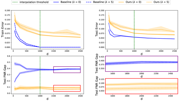
Figure 2: Results for the Waterbirds dataset [49]. Top row: Train error (left) and test error (right). The train error is used to identify the interpolation threshold for the baseline method (approximately $d=1000$). Bottom row: Comparing the FNR gap on the test set (left), with zoomed-in versions on the right.

6 Discussion and Additional Related Work

In terms of formal results, most existing guarantees about invariant learning algorithms rely on the assumption that infinite training data is available [3, 60, 57, 43, 45, 17]. Wang et al. [61], Chen et al. [11] analyze algorithms that bear resemblance to Algorithm 1 as they first project the data to a lower dimension and then fit a classifier. While these algorithms deal with more general assumptions in terms of the number of environments, number of spurious features, and noise distribution, the fact that their guarantees assume infinite data prevents them from being directly applicable to Algorithm 1. A few works with results on finite data are Ahuja et al. [2], Parulekar et al. [38] (and also Efroni et al. [19] who work on related problems in the context of sequential decision making) that characterize the sample complexity of methods that learn invariant classifiers. However, they do not analyze the overparameterized cases we are concerned with.

Negative results about learning overparameterized robust classifiers have been shown for methods based on importance weighting [66] and max-margin classifiers [50]. Our result is more general, applying to any learning algorithm that separates the data with arbitrarily small margins, instead of focusing on max-margin classifiers or specific algorithms. While we focus on the linear case, we believe it is instructive, as any reasonable method is expected to succeed in that case. Nonetheless, we believe our results can be extended to non-linear classifiers, and we leave this to future work.

One take-away from our result is that while low training loss is generally desirable, overfitting to the point of interpolation can significantly hinder invariance-inducing objectives. This means one cannot assume a typical deep learning model with an added invariance penalty will indeed achieve any form of invariance; this fact also motivates using held-out data for imposing invariance, as in our Algorithm 1 as well as several other two-stage approaches mentioned above.

Our work focuses theory underlying a wide array of algorithms, and there are natural follow-up topics to explore. One is to conduct a comprehensive empirical comparison of two-stage methods along with other methods that avoid interpolation, e.g., by subsampling data [24, 10]. Another interesting topic is whether there are other model properties that are incompatible with interpolation. For instance, recent work [9] connects the generalization gap and calibration error on the training distribution. We also note that our focus in this paper was not on types of invariance that are satisfiable by using clever data augmentation techniques (e.g. invariance to image translation), or the design of special architectures (e.g. [13, 30, 35]). These methods carefully incorporate a-priori known invariances, and their empirical success when applied to large models may suggest that there are lessons to be learned for the type of invariant learning considered in our paper. These connections seem like an exciting avenue for future research.

Appendix A Setting and Helper Lemmas

A.1 Notation

Let $\mathbb{U}(\mathrm{O}(d))$ be the uniform distribution over $d\times d$ orthogonal matrices, $\mathrm{Rad}(\alpha)$ the Rademacher distribution with parameter $\alpha$, and $\mathcal{N}({\bm{\mu}},\Sigma)$ the Gaussian and multivariate normal distribution with mean ${\bm{\mu}}$ and covariance $\Sigma$ (the dimension will be clear from context) and $W(\Sigma,d)$ the Wishart distribution with scale matrix $\Sigma$ and $d$ degrees of freedom. For the dataset $S=\{{\mathbf{x}}_{i},y_{i}\}_{i=1}^{N}$ we denote the indices of examples with set $\bar{S}=[N]$, and recalling that $S$ comprises two datasets $S_{1},S_{2}$, we denote the indices of their respective examples within $S$ by $\bar{S}_{1},\bar{S}_{2}\subseteq{\bar{S}}$ where $|\bar{S}_{e}|=N_{e}$ for $e\in{\{1,2\}}$. Our generative process is then:

$${\mathbf{U}} \sim\mathbb{U}(\mathrm{O}(d))$$

$${\bm{\mu}}_{c} =U_{1}\cdot r_{c},{\bm{\mu}}_{s}=U_{2}\cdot r_{s}$$

$$y_{i} =\mathrm{Rad}(\frac{1}{2}),n_{i}\sim\mathcal{N}(0,\sigma^{2}{\mathbf{I}}_{d})\quad\forall i\in{[N]}$$

$${\mathbf{x}}_{i} =y_{i}{\bm{\mu}}_{c}+y_{i}\theta_{e}{\bm{\mu}}_{s}+n_{i}\quad\forall e,i\in{\bar{S}_{e}}.$$

.

The vectors $E_{1},E_{2}\in{\{0,1\}^{N}}$ are binary vectors where $[E_{e}]_{i}=1$ for $i\in{\bar{S}_{e}}$ and $e\in{\{1,2\}}$, while $\mathbf{1}$ is the vector of length $N$ whose entries equal $1$. We also denote ${\mathbf{z}}_{i}={\mathbf{x}}_{i}y_{i}$ for $i\in{\bar{S}}$ and ${\mathbf{Z}}=[{\mathbf{z}}_{1},\ldots,{\mathbf{z}}_{N}]^{\top}\in{\mathbb{R}^{N\times d}}$ the matrix that stacks all these vectors. The $i$-th column of a matrix ${\mathbf{M}}$ is denoted by $M_{i}$, $s_{\min}({\mathbf{M}}),s_{\max}({\mathbf{M}})$ are its smallest and largest singular values accordingly. The unit matrix of size $n$ is denoted by ${\mathbf{I}}_{n}$ and for convenience we denote the direction of any vector ${\mathbf{v}}$ as $\hat{{\mathbf{v}}}:=\frac{{\mathbf{v}}}{\|{\mathbf{v}}\|}$. Finally, for some vector of coefficients ${\bm{\beta}}\in{\mathbb{R}^{N}}$, we will use the form $\hat{{\mathbf{w}}}=\sum_{i\in{\bar{S}}}{\beta_{i}y_{i}{\mathbf{x}}_{i}}+{\mathbf{w}}_{\perp}$ where ${\mathbf{w}}_{\perp}$ is in the orthogonal complement of ${\mathrm{span}(\{{\mathbf{x}}_{i}\}_{i\in{\bar{S}}})}$, to write any linear model (here normalized to unit norm).

For convenience we will write our proofs for the case where $\theta_{1}=1$ and $\sigma^{2}=d^{-1}$, extensions to different settings of these parameters are straightforward but result in a more cumbersome notation.

A.2 Operator Norms of Wishart Matrices

We begin with stating the required events for our results and their occurrence with high-probability:

Lemma 1.

Consider the matrix ${\mathbf{G}}={\mathbf{Z}}-{\mathbf{1}}{\bm{\mu}}_{c}^{\top}-(E_{1}+\theta_{2}E_{2}){\bm{\mu}}_{s}^{\top}$. For any $t>0$, with probability at least $1-6\exp(-t^{2}/2)$ the following hold simultaneously:

$$1-\sqrt{\frac{N}{d}}-\frac{t}{\sqrt{d}}\leq s_{\min}({\mathbf{G}}^{\top}) \leq s_{\max}({\mathbf{G}}^{\top})\leq 1+\sqrt{\frac{N}{d}}+\frac{t}{\sqrt{d}}$$ (8)

$$\|{\mathbf{G}}{\bm{\mu}}_{c}\| \leq t\sqrt{\frac{N}{d}}\|{\bm{\mu}}_{c}\|$$ (9)

$$\|{\mathbf{G}}{\bm{\mu}}_{s}\| \leq t\sqrt{\frac{N}{d}}\|{\bm{\mu}}_{s}\|$$ (10)

Proof.

${\mathbf{G}}$ is a random Gaussian matrix with $G_{i,j}\sim\mathcal{N}(0,d^{-1}{\mathbf{I}}_{N})$. By concentration results for random Gaussian matrices [59, Cor. 5.35] we obtain that with probability at least $1-2\exp(-t^{2}/2)$ Equation (8) holds.

Next we note that ${\mathbf{G}}{\bm{\mu}}_{c}\sim\mathcal{N}(0,d^{-1}\|{\bm{\mu}}_{c}\|^{2}{\mathbf{I}}_{N})$ and similarly for ${\mathbf{G}}{\bm{\mu}}_{s}$. The norm of a Gaussian random vector can be bounded for any $t_{2}>0$:

$${\mathbb{P}}\left[\|{\mathbf{G}}{\bm{\mu}}_{c}\|\geq t_{2}\right]\leq 2\exp\left(-\frac{dt_{2}^{2}}{2N\|{\bm{\mu}}_{c}\|^{2}}\right)$$

Setting $t_{2}=t\sqrt{\frac{N}{d}}\|{\bm{\mu}}_{c}\|$ we get that with probability at least $1-2\exp(-t^{2}/2)$ Equation (9) holds. Repeating the analogous derivation for Equation (10) and taking a union bound over the $3$ events, we arrive at the desired result. ∎

Lemma 2.

Conditioned on the events in Lemma 1 with parameter $t\geq 0$, if

$$\frac{\sqrt{N}+t}{\sqrt{d}}+\sqrt{N}(\|{\bm{\mu}}_{c}\|+\|{\bm{\mu}}_{s}\|)\leq\frac{1}{2},$$ (11)

then

$$\|{\mathbf{Z}}{\mathbf{Z}}^{\top}-\mathbb{E}[{\mathbf{Z}}{\mathbf{Z}}^{\top}]\|_{\mathrm{op}}\leq 3\frac{\sqrt{N}+t}{\sqrt{d}}~{}~{}\mbox{and}~{}~{}\frac{1}{2}I_{N}\preceq{\mathbf{Z}}{\mathbf{Z}}^{\top}\preceq 2I_{N}.$$

We note that we already assume $d\gg N$ and $\|{\bm{\mu}}_{c}\|\ll N^{-1/2}$, hence the additional assumption introduced in the conditions of this lemma is regarding the size of $\|{\bm{\mu}}_{s}\|\sqrt{N_{1}}$.

Proof.

Since ${\mathbf{G}}{\mathbf{G}}^{\top}\sim W(d^{-1}{\mathbf{I}}_{N},d)$ we have that $\mathbb{E}[{\mathbf{G}}{\mathbf{G}}^{\top}]={\mathbf{I}}_{N}$. Then from Equation (8) we can also obtain $(1-\sqrt{\frac{N}{d}}-\frac{t}{\sqrt{d}})^{2}\,{\mathbf{I}}_{n}\preceq{\mathbf{G}}{\mathbf{G}}^{\top}\preceq(1+\sqrt{\frac{N}{d}}+\frac{t}{\sqrt{d}})^{2}\,{\mathbf{I}}_{n}$, which leads to:

$$\left\|{\mathbf{G}}{\mathbf{G}}^{\top}-\mathbb{E}[{\mathbf{G}}{\mathbf{G}}^{\top}]\right\|_{\mathrm{op}}\leq\left(1+\sqrt{\frac{N}{d}}+\frac{t}{\sqrt{d}}\right)^{2}-1.$$

Combining this with Equation (9) and Equation (10)

$$\|{\mathbf{Z}}{\mathbf{Z}}^{\top}-\mathbb{E}\left[{\mathbf{Z}}{\mathbf{Z}}^{\top}\right]\|_{\mathrm{op}} \leq\|{\mathbf{G}}{\mathbf{G}}^{\top}-\mathbb{E}\left[{\mathbf{G}}{\mathbf{G}}^{\top}\right]\|_{\mathrm{op}}+\|{\mathbf{G}}{\bm{\mu}}_{c}{\mathbf{1}}^{\top}\|_{\mathrm{op}}+\|{\mathbf{G}}{\bm{\mu}}_{s}\left(E_{1}+\theta_{2}E_{2}\right)^{\top}\|_{\mathrm{op}}$$

$$\leq\sqrt{\frac{N}{d}}\left(2\frac{\sqrt{N}+t}{\sqrt{N}}+\frac{(\sqrt{N}+t)^{2}}{\sqrt{Nd}}+t\sqrt{N}(\|{\bm{\mu}}_{c}\|+\|{\bm{\mu}}_{s}\|)\right)$$

$$\leq\frac{\sqrt{N}+t}{\sqrt{d}}\left(2+\frac{\sqrt{N}+t}{\sqrt{d}}+\frac{t}{\sqrt{N}+t}\sqrt{N}(\|{\bm{\mu}}_{c}\|+\|{\bm{\mu}}_{s}\|)\right)$$

$$\leq\frac{\sqrt{N}+t}{\sqrt{d}}\cdot 2.5,$$

where the last transition follows from substituting Equation (11). To obtain the spectral bound on ${\mathbf{Z}}{\mathbf{Z}}^{\top}$ we have that ${\mathbf{Z}}={\mathbf{G}}+{\mathbf{1}}{\bm{\mu}}_{c}^{\top}+(E_{1}+\theta_{2}E_{2}){\bm{\mu}}_{s}^{\top}$. From Weyl’s inequality for singular values:

$$|s_{\mathrm{min}}({\mathbf{G}}^{\top}+{\bm{\mu}}_{c}{\mathbf{1}}^{\top}+ {\bm{\mu}}_{s}\left(E_{1}+\theta_{2}E_{2}\right)^{\top})-s_{\mathrm{min}}({\mathbf{G}}^{\top})|\leq$$

$$s_{\mathrm{max}}({\bm{\mu}}_{c}{\mathbf{1}}^{\top}+{\bm{\mu}}_{s}\left(E_{1}+\theta_{2}E_{2}\right)^{\top})\leq\|{\bm{\mu}}_{c}\|\sqrt{N}+\|{\bm{\mu}}_{s}\|\sqrt{N}.$$

Taken together with Equation (8) and the assumption in Equation (11) we get:

$$s_{\mathrm{min}}({\mathbf{Z}}^{\top}) \geq s_{\mathrm{min}}({\mathbf{G}}^{\top})-\|{\bm{\mu}}_{c}\|\sqrt{N}-\|{\bm{\mu}}_{s}\|\sqrt{N}$$

$$\geq 1-\frac{1}{\sqrt{d}}\left(\sqrt{N}+t\right)-\|{\bm{\mu}}_{c}\|\sqrt{N}-\|{\bm{\mu}}_{s}\|\sqrt{N}$$

$$\geq\frac{1}{2}.$$

To prove that ${\mathbf{Z}}{\mathbf{Z}}^{\top}\preceq 2$ we simply need to follow the same steps while taking notice that Weyl’s inequality also holds for $s_{\mathrm{max}}({\mathbf{G}}^{\top})$. This will give us $s_{\mathrm{max}}({\mathbf{Z}}^{\top})\leq 3/2\leq 2$ from which the upper bound follows. ∎

A.3 Sufficiency of Linear Classifiers Spanned by Data Points

We wish to bound $\langle\hat{{\mathbf{w}}}_{\bot},{\bm{\mu}}_{c}\rangle=r_{c}\langle\hat{{\mathbf{w}}}_{\perp},U_{1}\rangle$. To this end let us take an orthonormal basis $\{{\mathbf{v}}_{1},\ldots,{\mathbf{v}}_{N}\}$ and let these vectors form the columns of the orthogonal matrix $V\in\mathbb{R}^{d\times N}$. Let $P_{V}$ be the orthogonal projection matrix on the columns of $V$. We first claim that conditioned on the data, the component of the mean vectors that is not spanned by the data is distributed uniformly.

Lemma 3.

Let ${\bm{\mu}}^{\perp}_{c}\coloneqq(I-P_{V}){\bm{\mu}}_{c}$ and ${\bm{\mu}}^{\perp}_{s}\coloneqq(I-P_{V}){\bm{\mu}}_{c}$. Conditional on the training set $\{{\mathbf{x}}_{i},y_{i}\}_{i\in{S}}$, the vectors $\frac{{\bm{\mu}}^{\perp}_{s}}{\|{\bm{\mu}}^{\perp}_{s}\|}$ and $\frac{{\bm{\mu}}^{\perp}_{c}}{\|{\bm{\mu}}^{\perp}_{c}\|}$ are uniformly distributed on unit spheres a subspace of dimension $d-N$.

Proof.

Recalling the notation ${\mathbf{z}}_{i}=y_{i}{\mathbf{x}}_{i}$, note that $\{{\mathbf{z}}_{i}\}_{i\in\bar{S}}$ are sufficient statistics for ${\bm{\mu}}_{s},{\bm{\mu}}_{c}$ given the training data, i.e., $\mathbb{P}({\bm{\mu}}_{s},{\bm{\mu}}_{c}\mid\{{\mathbf{z}}_{i}\}_{i\in\bar{S}})=\mathbb{P}({\bm{\mu}}_{s},{\bm{\mu}}_{c}\mid\{{\mathbf{x}}_{i},y_{i}\}_{i\in\bar{S}})$. Furthermore, since the joint distribution of ${\bm{\mu}}_{s},{\bm{\mu}}_{c},\{{\mathbf{z}}_{i}\}_{i\in\bar{S}}$ is rotationally invariant, we have

$$\mathbb{P}({\bm{\mu}}_{s},{\bm{\mu}}_{c}\mid\{{\mathbf{z}}_{i}\}_{i\in\bar{S}})=\mathbb{P}({\mathbf{R}}{\bm{\mu}}_{s},{\mathbf{R}}{\bm{\mu}}_{c}\mid\{{\mathbf{R}}{\mathbf{z}}_{i}\}_{i\in\bar{S}})$$

for any orthogonal matrix ${\mathbf{R}}\in\mathbb{R}^{d\times d}$. Focusing on matrices ${\mathbf{R}}$ that presereve that data, i.e., satisfying ${\mathbf{R}}{\mathbf{z}}_{i}={\mathbf{z}}_{i}$ for all $i\in[N]$, we have

$$\mathbb{P}({\bm{\mu}}_{s},{\bm{\mu}}_{c}\mid\{{\mathbf{z}}_{i}\}_{i\in\bar{S}})=\mathbb{P}({\mathbf{R}}{\bm{\mu}}_{s},{\mathbf{R}}{\bm{\mu}}_{c}\mid\{{\mathbf{z}}_{i}\}_{i\in\bar{S}}).$$

We may also write this equality as

$$\mathbb{P}(P_{V}{\bm{\mu}}_{s},P_{V}{\bm{\mu}}_{c},(I-P_{V}){\bm{\mu}}_{s},(I-P_{V}){\bm{\mu}}_{c}\mid\{{\mathbf{z}}_{i}\}_{i\in\bar{S}})$$

$$\hskip 16.0pt=\mathbb{P}(P_{V}{\mathbf{R}}{\bm{\mu}}_{s},P_{V}{\mathbf{R}}{\bm{\mu}}_{c},(I-P_{V}){\mathbf{R}}{\bm{\mu}}_{s},(I-P_{V}){\mathbf{R}}{\bm{\mu}}_{c}\mid\{{\mathbf{z}}_{i}\}_{i\in\bar{S}}).$$

The fact that $R$ preserves $\{{\mathbf{z}}_{i}\}_{i\in\bar{S}}$ implies that $P_{V}{\mathbf{R}}=P_{V}={\mathbf{R}}P_{V}$ and therefore

$$\mathbb{P}(P_{V}{\bm{\mu}}_{s},P_{V}{\bm{\mu}}_{c},{\bm{\mu}}^{\perp}_{s},{\bm{\mu}}^{\perp}_{c}\mid\{{\mathbf{z}}_{i}\}_{i\in\bar{S}})=\mathbb{P}(P_{V}{\bm{\mu}}_{s},P_{V}{\bm{\mu}}_{c},{\mathbf{R}}{\bm{\mu}}^{\perp}_{s},{\mathbf{R}}{\bm{\mu}}^{\perp}_{c}\mid\{{\mathbf{z}}_{i}\}_{i\in\bar{S}}).$$

Marginalizing $P_{V}{\bm{\mu}}_{s},P_{V}{\bm{\mu}}_{c}$, we obtain that, conditional on the training data, the distribution of ${\bm{\mu}}^{\perp}_{s},{\bm{\mu}}^{\perp}_{c}$, is invariant to rotations that preserve the training data. Therefore, the unit vectors in the directions of ${\bm{\mu}}^{\perp}_{s}$ and ${\bm{\mu}}^{\perp}_{c}$ must each be uniformly distributed on the sphere orthogonal to the training data, which has dimension $d-N$. ∎

Now we simply need to derive a bound on $\langle{\mathbf{w}}_{\perp},{\bm{\mu}}_{s}\rangle$:

Corollary 1.

For any $t>0$ as in Lemma 1, with probability at least $1-10\exp(-t^{2}/2)$, all the events in Lemma 1 hold and additionally

$$\left|\langle{\mathbf{w}}_{\perp},{\bm{\mu}}_{s}\rangle\right|<\frac{\|{\bm{\mu}}_{s}\|}{\sqrt{d-N}}t~{}~{}\mbox{and}~{}~{}\left|\langle{\mathbf{w}}_{\perp},{\bm{\mu}}_{c}\rangle\right|<\frac{\|{\bm{\mu}}_{c}\|}{\sqrt{d-N}}t.$$ (12)

Proof.

Note that

$$\left|\langle{\mathbf{w}}_{\perp},{\bm{\mu}}_{s}\rangle\right|=\left|\langle{\mathbf{w}}_{\perp},{\bm{\mu}}^{\perp}_{s}\rangle\right|=\|{\bm{\mu}}^{\perp}_{s}\|\|{\mathbf{w}}_{\perp}\|\left|\left\langle\frac{{\mathbf{w}}_{\perp}}{\|{\mathbf{w}}_{\perp}\|},\frac{{\bm{\mu}}^{\perp}_{s}}{\|{\bm{\mu}}^{\perp}_{s}\|}\right\rangle\right|\leq\|{\bm{\mu}}_{s}\|\left|\left\langle\frac{{\mathbf{w}}_{\perp}}{\|{\mathbf{w}}_{\perp}\|},\frac{{\bm{\mu}}^{\perp}_{s}}{\|{\bm{\mu}}^{\perp}_{s}\|}\right\rangle\right|.$$

Conditional on the training data and the algorithm’s randomness, $\frac{{\mathbf{w}}_{\perp}}{\|{\mathbf{w}}_{\perp}\|}$ is a fixed unit vector in the subspace orthogonal to the training data (of dimension $d-N$), while $\frac{{\bm{\mu}}^{\perp}_{s}}{\|{\bm{\mu}}^{\perp}_{s}\|}$ is a spherically uniform unit vector in that subspace. Therefore, standard concentration bounds [4, Lemma 2.2] imply that, for any $t_{2}>0$

$$\mathbb{P}\left(\left|\left\langle\frac{{\mathbf{w}}_{\perp}}{\|{\mathbf{w}}_{\perp}\|},\frac{{\bm{\mu}}^{\perp}_{s}}{\|{\bm{\mu}}^{\perp}_{s}\|}\right\rangle\right|\geq t_{2}\right)\leq 2\exp(-(d-N)t_{2}^{2}/2).$$

The claimed result follows by taking $t_{2}=t/\sqrt{d-N}$, applying the same argument for ${\bm{\mu}}_{c}$ and taking a union bound. ∎

Appendix B Proofs of Main Result

In this section, we provide the proof of Proposition 1, our main theoretical finding highlighting a fundamental limitation to the robustness of any interpolating classifier. Following the notation of Appendix A, we write a general unit-vector classifier as $\hat{{\mathbf{w}}}=\sum_{i\in S}\beta_{i}{\mathbf{z}}_{i}+{\mathbf{w}}_{\perp}$, where ${\mathbf{z}}_{i}=y_{i}{\mathbf{x}}_{i}$. As explained in the proof sketch at Section 3, in order to show a lower bound on robust accuracy, we show a lower bound on the spurious-to-core ratio $\frac{\langle{\mathbf{w}},{\bm{\mu}}_{s}\rangle}{\langle{\mathbf{w}},{\bm{\mu}}_{c}\rangle}$ or equivalently upper bound $\frac{\langle{\mathbf{w}},{\bm{\mu}}_{s}\rangle}{\langle{\mathbf{w}},{\bm{\mu}}_{c}\rangle}$, which we can write as

$$\frac{\langle{\mathbf{w}},{\bm{\mu}}_{c}\rangle}{\langle{\mathbf{w}},{\bm{\mu}}_{s}\rangle}=\frac{\langle\hat{{\mathbf{w}}},{\bm{\mu}}_{c}\rangle}{\langle\hat{{\mathbf{w}}},{\bm{\mu}}_{s}\rangle}=\frac{\|{\bm{\mu}}_{c}\|^{2}}{\|{\bm{\mu}}_{s}\|^{2}}\cdot\frac{{\mathbf{1}}^{\top}\beta+\frac{1}{\|{\bm{\mu}}_{c}\|^{2}}\left[\sum_{i\in{\bar{S}}}{\beta_{i}\langle n_{i},{\bm{\mu}}_{c}\rangle+\langle{\mathbf{w}}_{\perp},{\bm{\mu}}_{c}\rangle}\right]}{(E_{1}+\theta_{2}E_{2})^{\top}\beta+\frac{1}{\|{\bm{\mu}}_{s}\|^{2}}\left[\sum_{i\in{\bar{S}}}{\beta_{i}\langle n_{i},{\bm{\mu}}_{s}\rangle}+\langle{\mathbf{w}}_{\perp},{\bm{\mu}}_{s}\rangle\right]}.$$ (13)

We develop the lower bound - and prove Proposition 1 - in three steps, each corresponsding to a subsection below. First, we give a lower bound on $(E_{1}+\theta_{2}E_{2})^{\top}{\bm{\beta}}$ using Lagrange duality (Lemma 4). Second, in Lemma 5, we bound the residual terms of the form $\frac{1}{\|{\bm{\mu}}\|^{2}}\left|\sum_{i\in{\bar{S}}}{\beta_{i}\langle n_{i},{\bm{\mu}}\rangle}+\langle{\mathbf{w}}_{\perp},{\bm{\mu}}\rangle\right|$ (for ${\bm{\mu}}\in\{{\bm{\mu}}_{c},{\bm{\mu}}_{s}\}$) using concentration of measure arguments from Appendix A. Finally, we combine these two results with the conditions of Proposition 1 to conclude its proof.

B.1 Lower bounding $(E_{1}+\theta_{2}E_{2})^{\top}{\bm{\beta}}$

The crux of our proof is showing that the term $(E_{1}+\theta_{2}E_{2})^{\top}{\bm{\beta}}$, i.e., the sum of the contributions of elements from the first environment to ${\mathbf{w}}$, must grow roughly as $N_{1}\gamma$ for any interpolating classifier. This will in turn imply a large spurious component in the classifier via manipulation of Equation (13).

Lemma 4.

Conditional on the events in Corollary 1 (with parameter $t>0$), if Equation (11) holds and ${\mathbf{w}}$ has normalized margin at least $\gamma$, we have that

$$(E_{1}+\theta_{2}E_{2})^{\top}{\bm{\beta}}\geq\frac{1}{2}\Bigg{(}(N_{1}+[\theta_{2}]_{+}N_{2})\gamma -\sqrt{2N_{2}}N_{1}\|{\bm{\mu}}_{c}\|^{2}$$

$$-\sqrt{18N}\cdot\frac{\sqrt{N}+t}{\sqrt{d}}-\sqrt{8N_{2}}\left[-\theta_{2}\right]_{+}\Bigg{)},$$ (14)

where $\left[z\right]_{+}=\max\{x,0\}$ denotes the positive part of $x$.

Proof of Lemma 4.

Our strategy for bounding $(E_{1}+\theta_{2}E_{2})^{\top}{\bm{\beta}}$ begins with writing down the smallest value it can reach for any unit-norm classifier $\hat{{\mathbf{w}}}$ with normalized margin at least $\gamma$. Recalling that $\hat{{\mathbf{w}}}={\mathbf{Z}}^{\top}{\bm{\beta}}+{\mathbf{w}}_{\perp}$ (for ${\mathbf{w}}_{\perp}$ such that ${\mathbf{Z}}{\mathbf{w}}_{\perp}=0$), the smallest possible value of $E_{1}^{\top}{\bm{\beta}}$ is the solution to the following optimization problem:

$$\min_{{\bm{\beta}}\in\mathbb{R}^{N},{\mathbf{w}}_{\perp}\in\ker({\mathbf{Z}})} ~{}(E_{1}+\theta_{2}E_{2})^{\top}{\bm{\beta}}$$ (15)

subject to $$\langle{{\mathbf{Z}}^{\top}{\bm{\beta}}+{\mathbf{w}}_{\perp}},y_{i}{\mathbf{x}}_{i}\rangle\geq\gamma~{}~{}\forall i\in[N]$$

$$\|{\mathbf{Z}}^{\top}{\bm{\beta}}+{\mathbf{w}}_{\perp}\|=1.$$

Since ${\mathbf{z}}_{i}=y_{i}{\mathbf{x}}_{i}$ and ${\mathbf{Z}}{\mathbf{w}}_{\perp}=0$, the first constraint is equivalent to the vector inequality $ZZ^{\top}{\bm{\beta}}\geq\gamma{\mathbf{1}}$, and the second constraint is equivalent to ${\bm{\beta}}^{\top}{\mathbf{Z}}{\mathbf{Z}}^{\top}{\bm{\beta}}=1-\|{\mathbf{w}}_{\perp}\|^{2}$. Relaxing the second constraint, the smallest value of $\left(E_{1}+\theta_{2}E_{2}\right)^{\top}{\bm{\beta}}$ is bounded from below by the solution to:

$$\min_{\beta\in{\mathbb{R}^{N}}} ~{}{\bm{\beta}}^{\top}(E_{1}+\theta_{2}E_{2})$$ (16)

subject to $${\mathbf{Z}}{\mathbf{Z}}^{\top}{\bm{\beta}}\geq\gamma\mathbf{1}$$

$${\bm{\beta}}^{\top}{\mathbf{Z}}{\mathbf{Z}}^{\top}\ {\bm{\beta}}\leq 1.$$

We now treat separately the two cases where $\theta_{2}\leq 0$ and $\theta_{2}>0$.

The case where $\theta_{2}\leq 0$.

Take Lagrange multipliers $\lambda\in{\mathbb{R}_{+}^{N}}$ and $\nu\geq 0$, from strong duality the above equals:

$$\max_{\lambda\in{\mathbb{R}_{+}^{N},\nu\geq 0}}\min_{\beta\in{\mathbb{R}^{N}}}{{\bm{\beta}}^{\top}(E_{1}+\theta_{2}E_{2})+\lambda^{\top}({\mathbf{1}}\gamma-{\mathbf{Z}}{\mathbf{Z}}^{\top}{\bm{\beta}})+\frac{1}{2}\nu}({\bm{\beta}}^{\top}{\mathbf{Z}}{\mathbf{Z}}^{\top}{\bm{\beta}}-1)$$

Optimizing the quadratic form over ${\bm{\beta}}$, the above becomes:

$$\max_{\lambda\in{\mathbb{R}_{+}^{N},\nu\geq 0}}{\lambda^{\top}{\mathbf{1}}\gamma-\frac{1}{2}\nu-\frac{1}{2}\left(E_{1}+\theta_{2}E_{2}-{\mathbf{Z}}{\mathbf{Z}}^{\top}\lambda\right)^{\top}\left(\nu{\mathbf{Z}}{\mathbf{Z}}^{\top}\right)^{-1}\left(E_{1}+\theta_{2}E_{2}-{\mathbf{Z}}{\mathbf{Z}}^{\top}\lambda\right)}$$

Maximizing over $\nu$ this becomes:

$$\max_{\lambda\in{\mathbb{R}_{+}^{N}}}{\lambda^{\top}{\mathbf{1}}\gamma-\sqrt{\left(E_{1}+\theta_{2}E_{2}-{\mathbf{Z}}{\mathbf{Z}}^{\top}\lambda\right)^{\top}\left({\mathbf{Z}}{\mathbf{Z}}^{\top}\right)^{-1}\left(E_{1}+\theta_{2}E_{2}-{\mathbf{Z}}{\mathbf{Z}}^{\top}\lambda\right)}}:=\max_{\lambda\in{\mathbb{R}_{+}^{N}}}{\mathcal{L}(\lambda)}$$ (17)

Thus, $(E_{1}+\theta_{2}E_{2})^{\top}{\bm{\beta}}$ is lower bounded by $\mathcal{L}(\lambda)$, for any $\lambda\in\mathbb{R}_{+}^{N}$. Taking $\lambda=\alpha E_{1}$ for $\alpha=\left(1+\left(\|{\bm{\mu}}_{c}\|^{2}+\|{\bm{\mu}}_{s}\|^{2}\right)N_{1}\right)^{-1}$, we obtain:

$$\mathcal{L}(\lambda) =N_{1}\gamma\alpha-\sqrt{\left(E_{1}+\theta_{2}E_{2}-\alpha{\mathbf{Z}}{\mathbf{Z}}^{\top}E_{1}\right)^{\top}\left({\mathbf{Z}}{\mathbf{Z}}^{\top}\right)^{-1}\left(E_{1}+\theta_{2}E_{2}-\alpha{\mathbf{Z}}{\mathbf{Z}}^{\top}E_{1}\right)}$$

$$\geq N_{1}\gamma\alpha-\sqrt{2}\|E_{1}+\theta_{2}E_{2}-\alpha{\mathbf{Z}}{\mathbf{Z}}^{\top}E_{1}\|$$

$$\geq N_{1}\gamma\alpha-\sqrt{2}\|E_{1}-\alpha{\mathbf{Z}}{\mathbf{Z}}^{\top}E_{1}\|-\sqrt{2N_{2}}|\theta_{2}|$$

$$=N_{1}\gamma\alpha-\sqrt{2}\|\left({\mathbf{I}}_{N}-\alpha\left(\mathbb{E}\left[{\mathbf{Z}}{\mathbf{Z}}^{\top}\right]+{\mathbf{Z}}{\mathbf{Z}}^{\top}-\mathbb{E}\left[{\mathbf{Z}}{\mathbf{Z}}^{\top}\right]\right)\right)E_{1}\|-\sqrt{2N_{2}}|\theta_{2}|$$

$$\geq N_{1}\gamma\alpha-\sqrt{2}\|\left({\mathbf{I}}_{N}-\alpha\mathbb{E}\left[{\mathbf{Z}}{\mathbf{Z}}^{\top}\right]\right)E_{1}\|-\sqrt{2}\|\alpha\left({\mathbf{Z}}{\mathbf{Z}}^{\top}-\mathbb{E}\left[{\mathbf{Z}}{\mathbf{Z}}^{\top}\right]\right)E_{1}\|-\sqrt{2N_{2}}|\theta_{2}|$$

Here, the first inequality is from our assumption that Equation (11) holds and hence ${\mathbf{Z}}{\mathbf{Z}}^{\top}\succeq\frac{1}{2}{\mathbf{I}}_{N}$ and the second is a triangle inequality. Recall the bound $\|{\mathbf{Z}}{\mathbf{Z}}^{\top}-\mathbb{E}\left[{\mathbf{Z}}{\mathbf{Z}}^{\top}\right]\|_{\mathrm{op}}\leq 3\frac{\sqrt{N}+t}{\sqrt{d}}$ from Lemma 2 and apply it to obtain:

$$\mathcal{L}(\lambda)\geq N_{1}\gamma\alpha-\sqrt{2}\|\left({\mathbf{I}}_{N}-\alpha\mathbb{E}\left[{\mathbf{Z}}{\mathbf{Z}}^{\top}\right]\right)E_{1}\|-\alpha-\alpha\sqrt{18N_{1}}\cdot\frac{\sqrt{N}+t}{\sqrt{d}}-\sqrt{2N_{2}}|\theta_{2}|$$

$$\geq N_{1}\gamma\alpha-\sqrt{2}\|\left({\mathbf{I}}_{N}-\alpha\mathbb{E}\left[{\mathbf{Z}}{\mathbf{Z}}^{\top}\right]\right)E_{1}\|-\alpha-\alpha\sqrt{18N}\cdot\frac{\sqrt{N}+t}{\sqrt{d}}-\sqrt{2N_{2}}|\theta_{2}|.$$

Let us break down the second term in the bound above:

$$\|\left({\mathbf{I}}_{N}-\alpha\mathbb{E}\left[{\mathbf{Z}}{\mathbf{Z}}^{\top}\right]\right)E_{1}\| =\|\left(1-\alpha-\alpha N_{1}\|{\bm{\mu}}_{s}\|^{2}\right)E_{1}-\alpha N_{1}\|{\bm{\mu}}_{c}\|^{2}{\mathbf{1}}\|$$

$$=\|\left(1-\alpha-\alpha N_{1}\|{\bm{\mu}}_{s}\|^{2}\right)E_{1}-\alpha N_{1}\|{\bm{\mu}}_{c}\|^{2}\left(E_{1}+E_{2}\right)\|$$

$$=\sqrt{\left(1-\alpha\left(1+N_{1}(\|{\bm{\mu}}_{s}\|^{2}+\|{\bm{\mu}}_{c}\|^{2}\right)\right)^{2}N_{1}+\alpha^{2}N_{1}^{2}\|{\bm{\mu}}_{c}\|^{4}N_{2}}$$

$$=\alpha N_{1}\|{\bm{\mu}}_{c}\|^{2}\sqrt{N_{2}},$$

where the final equality used $\alpha\left(1+N_{1}(\|{\bm{\mu}}_{s}\|^{2}+\|{\bm{\mu}}_{c}\|^{2}\right)=1$. Overall, we get:

$${\bm{\beta}}^{\top}(E_{1}+\theta_{2}E_{2})\geq\mathcal{L}(\lambda)\geq\alpha\left(N_{1}\gamma-\sqrt{2N_{2}}N_{1}\|{\bm{\mu}}_{c}\|^{2}-\sqrt{18N}\cdot\frac{\sqrt{N}+t}{\sqrt{d}}\right)-\sqrt{2N_{2}}|\theta_{2}|.$$ (18)

The proof is complete by noting that $\alpha\geq 1/2$ due to Equation (11).

The case where $\theta_{2}>0$.

Before introducing Lagrange multipliers, we revisit Equation 16 and this time we first bound the optimum from below as

$$\min_{{\bm{\beta}}\in{C({\mathbf{Z}},\gamma)}}{{\bm{\beta}}^{\top}(E_{1}+\theta_{2}E_{2})}\geq\theta_{2}\min_{{\bm{\beta}}\in{C({\mathbf{Z}},\gamma)}}{{\bm{\beta}}^{\top}(E_{1}+E_{2})}+(1-\theta_{2})\cdot\min_{{\bm{\beta}}\in{C({\mathbf{Z}},\gamma)}}{{\bm{\beta}}^{\top}E_{1}},$$

where we used $C({\mathbf{Z}},\gamma)$ as a shorthand for the constraints in Equation 16. By our derivation for the case of $\theta_{2}\leq 0$, the second term on the right hand side is readily bounded by the term in Equation 18 with $\theta_{2}=0$. We are left with bounding the first term, which turns out to be simpler since $E_{1}+E_{2}={\mathbf{1}}$. We repeat the process of taking the Lagrangian up until Equation 17, and now choose $\lambda=\alpha{\mathbf{1}}$ for $\alpha=\left(1+\left(\|{\bm{\mu}}_{c}\|^{2}+\|{\bm{\mu}}_{s}\|^{2}\right)N\right)^{-1}$. For completeness, let us rewrite the lower bound on the Lagrangian with these slight changes:

$$\mathcal{L}(\lambda) =N\gamma\alpha-\sqrt{\left({\mathbf{1}}-\alpha{\mathbf{Z}}{\mathbf{Z}}^{\top}{\mathbf{1}}\right)^{\top}\left({\mathbf{Z}}{\mathbf{Z}}^{\top}\right)^{-1}\left({\mathbf{1}}-\alpha{\mathbf{Z}}{\mathbf{Z}}^{\top}{\mathbf{1}}\right)}$$

$$\geq N\gamma\alpha-\sqrt{2}\|{\mathbf{1}}-\alpha{\mathbf{Z}}{\mathbf{Z}}^{\top}{\mathbf{1}}\|$$

$$=N\gamma\alpha-\sqrt{2}\|\left({\mathbf{I}}_{N}-\alpha\left(\mathbb{E}\left[{\mathbf{Z}}{\mathbf{Z}}^{\top}\right]+{\mathbf{Z}}{\mathbf{Z}}^{\top}-\mathbb{E}\left[{\mathbf{Z}}{\mathbf{Z}}^{\top}\right]\right)\right){\mathbf{1}}\|$$

$$\geq N\gamma\alpha-\sqrt{2}\|\left({\mathbf{I}}_{N}-\alpha\mathbb{E}\left[{\mathbf{Z}}{\mathbf{Z}}^{\top}\right]\right){\mathbf{1}}\|-\sqrt{2}\|\alpha\left({\mathbf{Z}}{\mathbf{Z}}^{\top}-\mathbb{E}\left[{\mathbf{Z}}{\mathbf{Z}}^{\top}\right]\right){\mathbf{1}}\|$$

Using again the bound on $\|{\mathbf{Z}}{\mathbf{Z}}^{\top}-\mathbb{E}\left[{\mathbf{Z}}{\mathbf{Z}}^{\top}\right]\|_{\mathrm{op}}$, the above bound becomes

$$\mathcal{L}(\lambda)\geq N\gamma\alpha-\sqrt{2}\|\left({\mathbf{I}}_{N}-\alpha\mathbb{E}\left[{\mathbf{Z}}{\mathbf{Z}}^{\top}\right]\right){\mathbf{1}}\|-\alpha-\alpha\sqrt{18N}\cdot\frac{\sqrt{N}+t}{\sqrt{d}}.$$

This time the chosen value for $\alpha$ makes the second term vanish, since

$$\|\left({\mathbf{I}}_{N}-\alpha\mathbb{E}\left[{\mathbf{Z}}{\mathbf{Z}}^{\top}\right]\right){\mathbf{1}}\| =\|\left(1-\alpha-\alpha N\left(\|{\bm{\mu}}_{s}\|^{2}+\|{\bm{\mu}}_{c}\|^{2}\right)\right){\mathbf{1}}\|=0.$$

Equation 11 again tells us that $\alpha>1/2$ which leads us to the bound:

$${\bm{\beta}}^{\top}(E_{1}+\theta_{2}E_{2})\geq\frac{1}{2}\Bigg{(}\gamma(\theta_{2}N+(1-\theta_{2})N_{1}) -(1-\theta_{2})\sqrt{2N_{2}}N_{1}\|\mu_{c}\|^{2}$$

$$-\sqrt{18}\left(\theta_{2}\sqrt{N}+(1-\theta_{2})\sqrt{N_{1}}\right)\cdot\frac{\sqrt{N}+t}{\sqrt{d}}\Bigg{)}$$

$$\geq\frac{1}{2}\Bigg{(}\gamma(\theta_{2}N_{2}+N_{1})-\sqrt{2N_{2}} N_{1}\|\mu_{c}\|^{2}-\sqrt{18N}\cdot\frac{\sqrt{N}+t}{\sqrt{d}}\Bigg{)}.$$

Combining the two cases for negative and positive $\theta_{2}$, we arrive at the desired bound in Lemma 4. ∎

B.2 Controlling residual terms

We now provide a bound on the terms in Equation (13) associated with quantities that vanish as the problem dimension grows.

Lemma 5.

Conditioned on all the events in Corollary 1 with parameter $t>0$ (which happen with probability at least $1-10\exp(-t^{2}/2)$) and the additional condition of Lemma 2, we have for ${\bm{\mu}}\in{\{{\bm{\mu}}_{c},{\bm{\mu}}_{s}\}}$:

$$\frac{1}{\|{\bm{\mu}}\|^{2}}\left|\sum_{i\in{\bar{S}}}{\beta_{i}\langle n_{i},{\bm{\mu}}\rangle}+\langle{\mathbf{w}}_{\perp},{\bm{\mu}}\rangle\right|\leq\frac{3t}{\|{\bm{\mu}}\|}\sqrt{\frac{{N}}{{d-N}}}$$ (19)

Proof.

We prove the claim for ${\bm{\mu}}_{s}$; the proof for ${\bm{\mu}}_{c}$ is analogous. Recall the random matrix ${\mathbf{G}}={\mathbf{Z}}-{\mathbf{1}}{\bm{\mu}}_{c}^{\top}-E_{1}{\bm{\mu}}_{s}^{\top}\in{\mathbb{R}^{N\times d}}$ from Lemma 1. From Equation (10) we get that $\|{\mathbf{G}}{\bm{\mu}}_{s}\|\leq t\sqrt{\frac{N}{d}}\|{\bm{\mu}}_{s}\|$ and then:

$$\sum_{i\in{\bar{S}}}{\beta_{i}\langle n_{i},{\bm{\mu}}_{s}\rangle}={\bm{\beta}}^{\top}{\mathbf{G}}{\bm{\mu}}_{s}\leq\|{\bm{\beta}}\|\|{\mathbf{G}}{\bm{\mu}}_{s}\|\leq t\|{\bm{\beta}}\|\sqrt{\frac{N}{d}}\|{\bm{\mu}}_{s}\|.$$

To eliminate $\|{\bm{\beta}}\|$ from this bound, we use ${\mathbf{Z}}{\mathbf{Z}}^{\top}\preceq\frac{1}{2}I_{N}$ due to Lemma 2 to write

$$\frac{1}{\sqrt{2}}\|{\bm{\beta}}\|\leq\sqrt{{\bm{\beta}}^{\top}{\mathbf{Z}}{\mathbf{Z}}^{\top}{\bm{\beta}}}\leq\sqrt{{\bm{\beta}}^{\top}{\mathbf{Z}}^{\top}{\mathbf{Z}}{\bm{\beta}}+\|{\mathbf{w}}_{\perp}\|^{2}}=\|\hat{{\mathbf{w}}}\|=1.$$

Finally, we use Equation (12) from Corollary 1 to bound $\left|\langle{\mathbf{w}}_{\perp},{\bm{\mu}}\rangle\right|$. ∎

B.3 Proof of Proposition 1

Proposition 1.

There are universal constants $c_{r}\in(0,1)$ and $C_{d},C_{r}\in(1,\infty)$, such that, for any target normalized $\gamma$, $\theta_{2}$ such that $\theta_{2}>-N_{1}\gamma/\sqrt{288N_{2}}$, and failure probability $\delta\in(0,1)$, if

$$\max\{r_{s}^{2},r_{c}^{2}\}\leq\frac{c_{r}}{N}~{}~{},~{}~{}\frac{r_{s}^{2}}{r_{c}^{2}}\geq C_{r}\left(1+\frac{\sqrt{N_{2}}}{(N_{1}+[\theta_{2}]_{+}N_{2})\gamma}\right)~{}~{}\mbox{ and}~{}~{}$$

$$d\geq C_{d}\frac{N}{\gamma^{2}N_{1}^{2}r_{c}^{2}}\log\frac{1}{\delta},$$

then with probability at least $1-\delta$ over the drawing of ${\bm{\mu}}_{c},{\bm{\mu}}_{s}$ and $(S_{1},S_{2})$ as described in Theorem  1, any $\hat{{\mathbf{w}}}\in{\mathbb{R}^{d}}$ that is a measurable function of $(S_{1},S_{2})$ and separates the data with normalized margin larger than $\gamma$ has robust error at least $0.5$.

Proof of Proposition 1.

Let $t\sqrt{10\log\frac{10}{\delta}}\geq\sqrt{2\log\frac{10}{\delta}}$, so that the events described in the previous lemmas and corollaries all hold with probability at least $1-\delta$. Note that for $c_{r}\leq 1/64$ we have

$$\sqrt{N}(\|{\bm{\mu}}_{c}\|+\|{\bm{\mu}}_{s}\|)\leq\frac{1}{4}$$ (20)

and (since $\gamma\leq\frac{1}{4\sqrt{N}}$)

$$d\geq\frac{C_{d}}{10}\frac{1}{\gamma^{2}}\frac{Nt^{2}}{N_{1}^{2}\|{\bm{\mu}}_{c}\|^{2}}\geq\frac{C_{d}}{10c_{r}}\frac{Nt^{2}}{N_{1}\gamma^{2}}\geq\frac{16C_{d}}{10c_{r}}\frac{N^{2}t^{2}}{N_{1}}N\geq\frac{6}{4}C_{d}Nt^{2}.$$

Consequently, for $C_{d}\geq 1$

$$\frac{\sqrt{N}+t}{\sqrt{d}}\leq 2\sqrt{\frac{1}{64C_{d}}}\leq\frac{1}{4}.$$ (21)

Combining Equations 20 and 21, we see that the condition in Equation (11) holds.

Therefore, we may apply Lemma 4; we now argue that under the assumptions of Proposition 1 the lower bound on $(E_{1}+\theta_{2}E_{2})^{\top}{\bm{\beta}}$ simplifies to a constant multiple of $N_{1}\gamma$. First, taking $c_{r}\leq 1/9$ and $C_{r}\geq 1$, we have

$$\sqrt{2N_{2}}N_{1}\|{\bm{\mu}}_{c}\|^{2}\leq\frac{\sqrt{2N_{2}}N_{1}\|{\bm{\mu}}_{s}\|^{2}}{C_{r}\left(1+\frac{\sqrt{N_{2}}}{N_{1}\gamma}\right)}\leq N_{1}\gamma\frac{\sqrt{2}N_{1}\|{\bm{\mu}}_{s}\|^{2}}{C_{r}}\leq N_{1}\gamma\frac{\sqrt{2}c_{r}}{C_{r}}\leq\frac{1}{6}N_{1}\gamma.$$

Second, using again $c_{r}\leq 1/64$ and taking $C_{d}\geq 180$,

$$\sqrt{18}\left([\theta_{2}]_{+}\sqrt{N}+(1-[\theta_{2}]_{+})\sqrt{N_{1}}\right)\frac{\sqrt{N}+t}{\sqrt{d}}\leq N_{1}\gamma\frac{\sqrt{18}}{\sqrt{C_{d}/10}}\frac{\sqrt{N}+t}{t\sqrt{N}}\sqrt{N}\|{\bm{\mu}}_{c}\|\leq\frac{1}{6}N_{1}\gamma.$$

Finally, due to our condition on $\theta_{2}$ in the proposition statement, we have $\sqrt{8N_{2}}\left[-\theta_{2}\right]_{+}\leq N_{1}\gamma/6$. Substituting all these into Equation (4), we conclude that under our assumptions $(E_{1}+\theta_{2}E_{2})^{\top}{\bm{\beta}}\geq\frac{1}{4}(N_{1}+[\theta_{2}]_{+}N_{2})\gamma$.

Next, we combine the lower bound on $(E_{1}+\theta_{2}E_{2})^{\top}{\bm{\beta}}$ with Lemma 5 to handle the denominator and numerator in the RHS of Equation (13). Beginning with the numerator, we have

$${\mathbf{1}}^{\top}{\bm{\beta}}+\frac{1}{r_{c}^{2}}\left[\sum_{i\in{\bar{S}}}{\beta_{i}\langle n_{i},{\bm{\mu}}_{c}\rangle}+\langle{\mathbf{w}}_{\perp},{\bm{\mu}}_{c}\rangle\right]\leq(E_{1}+\theta_{2}E_{2})^{\top}{\bm{\beta}}+(1-\theta_{2})\|E_{2}\|\|{\bm{\beta}}\|+\frac{3t}{r_{c}}\sqrt{\frac{N}{d-N}}.\\$$

As argued in the proof of Lemma 5, we have $\|{\bm{\beta}}\|\leq\sqrt{2}$ and therefore $(1-\theta_{2})\|E_{2}\|\|{\bm{\beta}}\|\leq\sqrt{8N_{2}}$. Substituting again our assumptions $d$ (which imply $d>2N$), and taking $C_{d}\geq 64\cdot 180$, we have

$$\frac{3t}{r_{c}}\sqrt{\frac{N}{d-N}}\leq\frac{\sqrt{18}t}{\|{\bm{\mu}}_{c}\|}\sqrt{d}\leq N_{1}\gamma\sqrt{\frac{180}{C_{d}}}\leq\frac{1}{8}N_{1}\gamma.$$

For the denominator, noting $\|{\bm{\mu}}_{c}\|\leq\|{\bm{\mu}}_{s}\|$ by our assumption, we may similarly write

$$(E_{1}+\theta_{2}E_{2})^{\top}{\bm{\beta}}+\frac{1}{\|{\bm{\mu}}_{s}\|^{2}}\left[\sum_{i\in{\bar{S}}}{\beta_{i}\langle n_{i},{\bm{\mu}}_{s}\rangle}+\langle{\mathbf{w}}_{\perp},{\bm{\mu}}_{s}\rangle\right]\geq(E_{1}+\theta_{2}E_{2})^{\top}{\bm{\beta}}-\frac{1}{8}N_{1}\gamma.$$

Consequently (since $(E_{1}+\theta_{2}E_{2})^{\top}{\bm{\beta}}\geq\frac{1}{4}N_{1}\gamma$), we have that the denominator is nonnegative. (If the numerator is not positive, ${\mathbf{w}}$ will have error greater than $1/2$ for $\theta=0$). Substituting back to Equation (13) and using the lower bound $(E_{1}+\theta_{2}E_{2})^{\top}{\bm{\beta}}\geq\frac{1}{4}N_{1}\gamma$, we get

$$\frac{\langle{\mathbf{w}},{\bm{\mu}}_{c}\rangle}{\langle{\mathbf{w}},{\bm{\mu}}_{s}\rangle}\frac{\|{\bm{\mu}}_{s}\|^{2}}{\|{\bm{\mu}}_{c}\|^{2}}\leq\frac{(E_{1}+\theta_{2}E_{2})^{\top}{\bm{\beta}}+\sqrt{8N_{2}}+\frac{1}{8}N_{1}\gamma}{(E_{1}+\theta_{2}E_{2})^{\top}{\bm{\beta}}-\frac{1}{8}N_{1}\gamma} \leq\frac{\frac{1}{4}\left(N_{1}+[\theta_{2}]_{+}N_{2}\right)\gamma+\sqrt{8N_{2}}+\frac{1}{8}N_{1}\gamma}{\frac{1}{4}\left(N_{1}+[\theta_{2}]_{+}N_{2}\right)\gamma-\frac{1}{8}N_{1}\gamma}$$

$$\leq 3+\frac{\sqrt{512N_{2}}}{\left(N_{1}+[\theta_{2}]_{+}N_{2}\right)\gamma}.$$

Therefore, for $C_{r}\geq 32$ we have $\frac{\langle{\mathbf{w}},{\bm{\mu}}_{s}\rangle}{\langle{\mathbf{w}},{\bm{\mu}}_{c}\rangle}\geq 1$ as required. Since the error of classifier ${\mathbf{w}}$ in environment with parameter $\theta$ is

$$Q\left(\frac{\langle{\mathbf{w}},{\bm{\mu}}_{c}\rangle}{\sigma\|{\mathbf{w}}\|}\left(1+\theta\frac{\langle{\mathbf{w}},{\bm{\mu}}_{s}\rangle}{\langle{\mathbf{w}},{\bm{\mu}}_{c}\rangle}\right)\right),$$

(where $Q(t):={\mathbb{P}}(\mathcal{N}(0;1)>t)$ is the Gaussian tail function), the fact that $\frac{\langle{\mathbf{w}},{\bm{\mu}}_{s}\rangle}{\langle{\mathbf{w}},{\bm{\mu}}_{c}\rangle}\geq 1$ implies that there exists $\theta\in[-1,1]$ for which the error is $Q(0)=0.5$, implying the stated bound on the robust error. ∎

Appendix C Lower Bounds On the Achievable Margin

We now argue that, in our model, a simple signed-sample-mean estimator interpolates the data with normalized margin scaling as $1/\sqrt{N}$. This fact establishes the first part of Theorem 1.

Proposition 3.

There exist universal constants $c_{r}^{\prime},C_{d}^{\prime}>0$ such that, in the Linear Two Environment Problem with parameters $N_{1},N_{2},d>0$, ${\bm{\mu}}_{c},{\bm{\mu}}_{s}\in\mathbb{R}^{d}$, $\theta_{1},\theta_{2}\in[-1,1]$ and $\sigma^{2}=1/d$, for any $\delta\in(0,1/2)$ if

$$\max\{r_{c},r_{s}\}\leq\frac{c_{r}^{\prime}}{N}~{}~{},~{}~{}\theta_{1}N_{1}\geq-\theta_{2}N_{2}~{}~{}\mbox{and}~{}~{}d\geq C_{d}^{\prime}N^{2}\log\left(\frac{1}{\delta}\right)$$

then with probability at least $1-\delta$, the signed-sample-mean estimator ${\mathbf{w}}_{\mathrm{mean}}=\frac{1}{N}\sum_{i=1}^{N}y_{i}x_{i}$ obtains normalized margin of at least $\frac{1}{\sqrt{8N}}$.

Proof.

Using the notation defined in the beginning of Appendix A, we note that ${\mathbf{w}}_{\mathrm{mean}}=\frac{1}{N}{\mathbf{Z}}^{\top}{\mathbf{1}}$ and (for $\sigma^{2}d=1$) its normalized margin is

$$\min_{i\in[N]}\frac{y_{i}\langle{\mathbf{x}}_{i},{\mathbf{w}}_{\mathrm{mean}}\rangle}{\|{\mathbf{w}}_{\mathrm{mean}}\|}=\min_{i\in[N]}\frac{[{\mathbf{Z}}{\mathbf{w}}_{\mathrm{mean}}]_{i}}{\|{\mathbf{w}}_{\mathrm{mean}}\|}=\min_{i\in[N]}\frac{[{\mathbf{Z}}{\mathbf{Z}}^{\top}{\mathbf{1}}]_{i}}{\|{\mathbf{Z}}^{\top}{\mathbf{1}}\|}.$$

Substituting the assumed bounds on $d$ and $\|{\bm{\mu}}_{c}\|,\|{\bm{\mu}}_{s}\|$ into Lemma 2 (with $t=\sqrt{8\log\frac{1}{\delta}}\geq\sqrt{2\log\frac{6}{\delta}}$), it is easy to verify that for sufficiently small $c_{r}^{\prime}$ and sufficiently large $C_{d}^{\prime}$, the condition in Equation (11) holds, and therefore

$$\|{\mathbf{Z}}{\mathbf{Z}}^{\top}-\mathbb{E}{\mathbf{Z}}{\mathbf{Z}}^{\top}\|_{\mathrm{op}}\leq 3\frac{\sqrt{N}+t}{\sqrt{d}}\leq\frac{1}{\sqrt{4N}},$$

with the final inequality following by choosing $C_{d}^{\prime}$ sufficiently large. Lemma 2 then also implies that ${\mathbf{Z}}{\mathbf{Z}}^{\top}\preceq 2I_{N}$.

Noting that $\mathbb{E}{\mathbf{Z}}{\mathbf{Z}}^{\top}=I_{N}+\|\mu_{c}\|^{2}{\mathbf{1}}{\mathbf{1}}^{\top}+\|\mu_{s}\|^{2}(\theta_{1}E_{1}+\theta_{2}E_{2})(\theta_{1}E_{1}+\theta_{2}E_{2})^{\top}$, we have that, for all $i\in[N]$,

$$[{\mathbf{Z}}{\mathbf{Z}}^{\top}{\mathbf{1}}]_{i}\geq[\mathbb{E}{\mathbf{Z}}{\mathbf{Z}}^{\top}{\mathbf{1}}]_{i}-\|{\mathbf{Z}}{\mathbf{Z}}^{\top}-\mathbb{E}{\mathbf{Z}}{\mathbf{Z}}^{\top}\|_{\mathrm{op}}\|{\mathbf{1}}\|\geq 1-\frac{1}{\sqrt{4N}}\|{\mathbf{1}}\|=\frac{1}{2}.$$

Moreover, ${\mathbf{Z}}{\mathbf{Z}}^{\top}\preceq 2I_{N}$ implies that

$$\|{\mathbf{Z}}^{\top}{\mathbf{1}}\|=\sqrt{{\mathbf{1}}^{\top}{\mathbf{Z}}{\mathbf{Z}}^{\top}{\mathbf{1}}}\leq 2\|{\mathbf{1}}\|=2\sqrt{N}.$$

Combining the above two displays yields the claimed margin bound. ∎

C.1 Margin for invariant classifiers

We now lower bound the margin achieved by the invariant classifier ${\bm{w}}={\bm{\mu}}_{c}$. To that end, note that $y_{i}\langle{\bm{\mu}}_{c},{\mathbf{x}}_{i}\rangle/\|{\bm{\mu}}_{c}\|\sim\mathcal{N}(\|{\bm{\mu}}_{c}\|;\sigma^{2})$ for all $i\in\bar{S}$. Therefore, taking $\sigma^{2}=1/d$, with probability at least $1-\delta$ we have, for all $i\in\bar{S}$

$$\frac{y_{i}\langle{\bm{\mu}}_{c},{\mathbf{x}}_{i}\rangle}{\|{\bm{\mu}}_{c}\|\sqrt{\sigma^{2}d}}\geq\|{\bm{\mu}}_{c}\|-\frac{1}{\sqrt{d}}Q^{-1}\left(\frac{\delta}{N}\right)\geq\|{\bm{\mu}}_{c}\|-\sqrt{\frac{2\log\frac{N}{\delta}}{d}}.$$

Substituting the choices

$$\|{\bm{\mu}}_{c}\|^{2}=\Theta\left(\frac{1}{N\left(1+\frac{\sqrt{N_{2}}}{N_{1}\gamma}\right)}\right)~{}~{}\mbox{and}~{}~{}d=\Omega\left(\frac{\log\frac{1}{\delta}}{N_{\min}^{2}\|{\bm{\mu}}_{s}\|^{4}}\right)\geq\Omega\left(\frac{\log\frac{N}{\delta}}{\|{\bm{\mu}}_{c}\|^{2}}\right)$$

form the proof of Theorem 1 (see Appendix E), we obtain that, with probability at least $1-\delta$, the normalized margin of $\mu_{c}$ is

$$\Omega(\|{\bm{\mu}}_{c}\|)=\Omega\left(\frac{1}{\sqrt{N\left(1+\frac{\sqrt{N_{2}}}{N_{1}\gamma}\right)}}\right)=\Omega\left(\min\left\{\frac{1}{\sqrt{N}},\sqrt{\frac{\gamma}{N_{2}}}\right\}\right).$$

In addition, letting $n_{i}\sim\mathcal{N}(0;\sigma^{2}{\mathbf{I}}_{d})$, we may also consider the invariant classifier

$${\bm{w}}={\bm{\mu}}_{c}+\frac{1}{N}\sum_{i=1}^{N}n_{i}=\frac{1}{N}\sum_{e\in\{1,2\}}\sum_{({\bm{x}},y)\in S_{i}}(y_{i}{\bm{x}}_{i}-\theta_{e}{\bm{\mu}}_{s}).$$

The proof of Proposition 3 (with $\theta_{1}=\theta_{2}=0$) shows that, under the assumptions of that proposition, the classifier ${\bm{w}}$ defined above attains margin of $\frac{1}{4\sqrt{N}}$ with high probability.

We emphasize once more that, while the discussion above shows the existence of invariant classifiers with good margin, our main results proves that these classifiers may be unlearnable from the finite samples $S_{1}$ and $S_{2}$. To show this existence numerically too, we run our simulations from Section 5 and add a model that is fitted on the features where ${\bm{\mu}}_{s}$ is removed (i.e. the new datapoints are ${\mathbf{x}}_{i}-\theta_{e}{\bm{\mu}}_{s}$ for each point ${\mathbf{x}}_{i}\in{S_{e}}$). We observe in Figure 5 that for a sufficiently large dimension the model is both interpolating and has high robust accuracy, demonstrating the existence discussed above. We emphasize again that this model cannot necessarily be learned by an algorithm that receives the original $(S_{1},S_{2})$ (before the removal of ${\bm{\mu}}_{s}$).

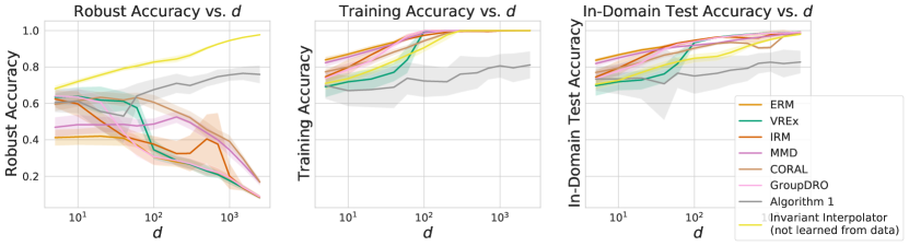
Figure 5: Simulation from Section 5 with an added model trained after removing the spurious feature. This demonstrated the existence of an invariant interpolator, yet our theoretical results suggest that this type of model cannot be learned by an interpolating learning rule

Appendix D Analysis of Algorithm 1

The proof that Algorithm 1 indeed achieves a non-trivial robust error will require some definitions and more mild assumptions which we now turn to describe.
Definitions. Denote the first-stage training set indices by $S$, where $|S|=N$ and second stage “fine-tuning” set by $|D|=M$. Let us denote:

$$\bar{{\mathbf{n}}}_{e} =\frac{1}{N_{e}}\sum_{i\in{S_{e}}}{n_{i}},~{}\bar{{\mathbf{m}}}_{e}=\frac{1}{M_{e}}\sum_{i\in{D_{e}}}{n_{i}},~{}\bar{{\mathbf{m}}}_{e,1}=\frac{1}{M_{e,1}}\sum_{i\in{D_{e,1}}}{n_{i}}.$$

Models will be defined by:

$${\mathbf{w}}_{e}:=\> \frac{1}{N_{e}}{\sum_{i\in{S_{e}}}{y_{i}{\mathbf{x}}_{i}}}=\mu_{c}+\theta_{e}\mu_{s}+\bar{{\mathbf{n}}}_{e},\quad e\in{\{1,2\}},$$

$$f_{{\mathbf{v}}}(x;S)=\> ~{}\langle v_{1}\cdot{\mathbf{w}}_{1}+v_{2}\cdot{\mathbf{w}}_{2},{\mathbf{x}}\rangle.$$

The Equalized Opportunity (EOpp) constraint is:

$$\hat{T}_{1}(f_{\mathbf{v}};D,S) =\hat{T}_{2}(f_{\mathbf{v}};D)$$

$$\hat{T}_{e}(f_{\mathbf{v}};D,S) =\frac{1}{M_{e,1}}\sum_{i\in{D_{e,1}}}{f_{\mathbf{v}}({\mathbf{x}}_{i})}$$

Additional Assumptions We assume w.l.o.g $\theta_{2}>\theta_{1}$, define $\Delta:=\theta_{2}-\theta_{1}>0$ and $r_{\mu}=\frac{\|\mu_{s}\|}{\|\mu_{c}\|}>1$. We consider $r_{\mu},\Delta$ as fixed numbers. That is, they do not depend on $N,d$ and other parameters of the problem. Also define $r:=\frac{\Delta\theta_{\max}}{\Delta+4\theta_{\max}}$, where $\theta_{\max}:=\mathrm{arg}{\max}\{|\theta_{1}|,|\theta_{2}|\}\leq 1$. The following additional assumptions will be required for our concentration bounds.

Assumption 1.

Let $t>0$ be a fixed user specified value, which we define later and will control the success probability of the algorithm. We will assume that for each $e\in{\{1,2\}}$ and some universal constants $c_{c},c_{s}>0$:

$$\|\mu_{s}\|^{2} \geq t\sigma^{2}c_{s}\max\left\{\frac{1}{r^{2}N_{e}},\frac{1}{(r\Delta)^{2}M_{e,1}},\frac{\sqrt{d}}{M_{e,1}r\Delta}\right\}$$

$$\|\mu_{c}\|^{2} \geq t\sigma^{2}c_{c}\max\left\{\frac{1}{\Delta^{2}N_{e}},\frac{r^{2}_{\mu}}{\left(\Delta^{2}M_{e,1}\right)},\frac{r_{\mu}^{2}}{\Delta^{2}M_{e}},\frac{\sqrt{d}}{M_{e,1}\Delta^{2}},\frac{\sqrt{d}}{M_{e}\Delta}\right\}$$

Analyzing the EOpp constraint. Writing the terms defined above in more detailed form gives:

$$\epsilon_{e}({\mathbf{v}})= \langle\bar{{\mathbf{m}}}_{e,1},v_{1}\left(\mu_{c}+\theta_{1}\mu_{s}+\bar{{\mathbf{n}}}_{1}\right)+v_{2}\left(\mu_{c}+\theta_{2}\mu_{s}+\bar{{\mathbf{n}}}_{2}\right)\rangle$$

$$\delta_{e}({\mathbf{v}})= \langle\bar{{\mathbf{m}}}_{e},v_{1}\left(\mu_{c}+\theta_{1}\mu_{s}+\bar{{\mathbf{n}}}_{1}\right)+v_{2}\left(\mu_{c}+\theta_{2}\mu_{s}+\bar{{\mathbf{n}}}_{2}\right)\rangle$$

$$\hat{T}_{e}(f_{{\mathbf{v}}};D,S)= (v_{1}+v_{2})\|\mu_{c}\|^{2}+(v_{1}\theta_{1}+v_{2}\theta_{2})\theta_{e}\|\mu_{s}\|^{2}+$$

$$\langle\mu_{c}+\theta_{e}\mu_{s},v_{1}\bar{{\mathbf{n}}}_{1}+v_{2}\bar{{\mathbf{n}}}_{2}\rangle+\epsilon_{e}({\mathbf{v}})$$

So the EOpp constraint is:

$$v_{1} \left[\theta_{1}\|\mu_{s}\|^{2}+\langle\bar{{\mathbf{n}}}_{1},\mu_{s}\rangle\right]\theta_{1}+v_{2}\left[\theta_{2}\|\mu_{s}\|^{2}+\langle\bar{{\mathbf{n}}}_{2},\mu_{s}\rangle\right]\theta_{1}+\epsilon_{1}({\mathbf{v}})=$$

$$v_{1}\left[\theta_{1}\|\mu_{s}\|^{2}+\langle\bar{{\mathbf{n}}}_{1},\mu_{s}\rangle\right]\theta_{2}+v_{2}\left[\theta_{2}\|\mu_{s}\|^{2}+\langle\bar{{\mathbf{n}}}_{2},\mu_{s}\rangle\right]\theta_{2}+\epsilon_{2}({\mathbf{v}})$$ (22)

Lemma 6.

Consider all the solutions ${\mathbf{v}}=(v_{1},v_{2})$ that satisfy EOpp and have $\|{\mathbf{v}}\|_{\infty}=1$. With probability $1$ there are exactly two such solutions ${\mathbf{v}}_{\mathrm{pos}},{\mathbf{v}}_{\mathrm{neg}}$, where ${\mathbf{v}}_{\mathrm{pos}}=-{\mathbf{v}}_{\mathrm{neg}}$.

We will consider ${\mathbf{v}}_{\mathrm{pos}}$ as the solution that satisfies $v_{\mathrm{pos},1}+v_{\mathrm{pos},2}>0$.

Proof.

Is it easy to see that the EOpp constraint is a linear equation in $v_{1},v_{2}$ and with probability $1$ the coefficients in this linear equations are nonzero. Therefore the solutions to this equation form a line in $\mathbb{R}^{2}$ that passes through the origin. Consequently, this line intersects the $l_{\infty}$ unit ball at two points, that we denote ${\mathbf{v}}_{\mathrm{pos}},{\mathbf{v}}_{\mathrm{neg}}$, which are negations of one another. ∎

The proposed algorithm. Now we can restate our algorithm in terms of $v_{\mathrm{pos}}$ and $v_{\mathrm{neg}}$ and analyze its retrieved solution.

• Calculate ${\mathbf{w}}_{1}$ and ${\mathbf{w}}_{2}$ according to their definitions.

• Consider the solutions $\{{\mathbf{v}}_{\mathrm{pos}},{\mathbf{v}}_{\mathrm{neg}}\}$ that satisfy EOpp and also $\|{\mathbf{v}}\|_{\infty}=1$.

• Return the solution: ${\mathbf{v}}\in{\{{\mathbf{v}}_{\mathrm{pos}},{\mathbf{v}}_{\mathrm{neg}}\}}$ which has the higher score, where the score is:

  $${\mathbf{v}}^{*}\in{\mathrm{arg}\max_{{\mathbf{v}}\in{\{{\mathbf{v}}_{\mathrm{pos}},{\mathbf{v}}_{\mathrm{neg}}\}}}{\sum_{i\in{D}}{\langle v_{1}{\mathbf{w}}_{1}+v_{2}{\mathbf{w}}_{2},y_{i}{\mathbf{x}}_{i}\rangle}}}$$

We first analyze the two possible solution $v_{\mathrm{pos}}$ and $v_{\mathrm{neg}}$ and show that their coordinates cannot be negations of each other. Intuitively, in an ideal scenario with infinite data, the EOpp constraint will enforce $v_{1}\theta_{1}=-v_{2}\theta_{2}$. Then $v_{1}=-v_{2}$ is only possible if $\theta_{1}=\theta_{2}$, which we assume is not the case (if it is, we cannot identify the spurious correlation from data). The assumption of a fixed $\Delta>0$, will let us show that indeed with high probability $v_{1}=-v_{2}$ does not occur.

Lemma 7.

Let $t>0$ and consider the solutions $v_{\mathrm{neg}},v_{\mathrm{pos}}$ that the algorithm may return. With probability at least $1-34\exp(-t^{2})$ , the solutions satisfy $|v_{1}+v_{2}|\geq\frac{\Delta}{2}$.

Proof.

Assume that for $e\in{\{1,2\}}$ the following events occur:

$$|\langle\bar{{\mathbf{n}}}_{e},\mu_{s}\rangle| \leq r\|\mu_{s}\|^{2}$$ (23)

$$|\langle\bar{{\mathbf{m}}}_{1,1}-\bar{{\mathbf{m}}}_{2,1},\mu_{c}+\theta_{e}\mu_{s}+\bar{{\mathbf{n}}}_{e}\rangle| \leq r\Delta\|\mu_{s}\|^{2}$$ (24)

Corollary 3 will show that they occur with the desired probability in our statement. Let us incorporate these events into the EOpp constraint. We group the items multiplied by $v_{1}$ and those multiplied by $v_{2}$:

$$-v^{*}_{1}\big{[}\theta_{1}\|\mu_{s}\|^{2}\Delta+\langle\bar{{\mathbf{n}}}_{1},\mu_{s}\rangle \Delta+\langle\bar{{\mathbf{m}}}_{1,1}-\bar{{\mathbf{m}}}_{2,1},\mu_{c}+\theta_{1}\mu_{s}+\bar{{\mathbf{n}}}_{1}\rangle\big{]}=$$

$$v^{*}_{2}\left[\theta_{2}\|\mu_{s}\|^{2}\Delta+\langle\bar{{\mathbf{n}}}_{2},\mu_{s}\rangle\Delta+\langle\bar{{\mathbf{m}}}_{2,1}-\bar{{\mathbf{m}}}_{1,1},\mu_{c}+\theta_{2}\mu_{s}+\bar{{\mathbf{n}}}_{2}\rangle\right]$$

Let us denote for convenience (where we drop the dependence on parameters in the notation):

$$a=\|\mu_{s}\|^{-2}\Delta\left(\langle\bar{{\mathbf{n}}}_{1},\mu_{s}\rangle+\Delta^{-1}\langle\bar{{\mathbf{m}}}_{1,1}-\bar{{\mathbf{m}}}_{2,1},\mu_{c}+\theta_{1}\mu_{s}+\bar{{\mathbf{n}}}_{1}\rangle\right)$$

$$b=\|\mu_{s}\|^{-2}\Delta\left(\langle\bar{{\mathbf{n}}}_{2},\mu_{s}\rangle+\Delta^{-1}\langle\bar{{\mathbf{m}}}_{2,1}-\bar{{\mathbf{m}}}_{1,1},\mu_{c}+\theta_{2}\mu_{s}+\bar{{\mathbf{n}}}_{2}\rangle\right)$$

Now the EOpp constraint can be written as $-v_{1}^{*}\|\mu_{s}\|^{2}\Delta\left(\theta_{1}+a\right)=v_{2}^{*}\|\mu_{s}\|^{2}\Delta\left(\theta_{2}+b\right)$. Plugging in Equation (23) and Equation (24), we see that $\max\{|a|,|b|\}\leq r$.

Assume that $|\theta_{1}+b|\geq|\theta_{2}+a|$, and note that since $\|{\mathbf{v}}^{*}\|_{\infty}=1$ we have that $|v_{1}^{*}|=1$ (the proof for the other case is analogous). We note that by definition $\Delta\leq 2\theta_{\max}$, hence if $v_{2}^{*}=0$ we have $|v_{1}^{*}+v_{2}^{*}|=1\geq\frac{\Delta}{2\theta_{\max}}$ and our claim holds. Otherwise, we can write:

$$|v_{1}^{*}+v_{2}^{*}| =\left|1-\frac{\theta_{2}+b}{\theta_{1}+a}\right|=\left|\frac{\Delta+a-b}{\theta_{1}+a}\right|\geq\frac{\Delta-2r}{\theta_{\max}+r}=\frac{\Delta-2\frac{\Delta\theta_{\max}}{\Delta+4\theta_{\max}}}{\theta_{\max}+\frac{\Delta\theta_{\max}}{\Delta+4\theta_{\max}}}$$

$$=\frac{\Delta\left(\Delta+4\theta_{\max}-2\theta_{\max}\right)}{\theta_{\max}\left(\Delta+4\theta_{\max}+\Delta\right)}=\frac{\Delta}{2\theta_{\max}}\geq\frac{\Delta}{2}$$

∎

The result above will be useful for proving the rest of our claims towards the performance guarantees of the algorithm. We first show that the retrieved solution is the one that is positively aligned with $\mu_{c}$.

Lemma 8.

With probability at least $1-34\exp(-t^{2})$ , between the two solutions considered at the second stage of our algorithm, the one with $v_{1}+v_{2}\geq 0$ achieves a higher score.

Proof.

Let’s write down the score on environment $e\in{\{1,2\}}$ in detail:

$$\sum_{i\in{D_{e}}}{{\mathbf{w}}^{\top}{\mathbf{x}}_{i}y_{i}}= (v_{1}+v_{2})\|\mu_{c}\|^{2}+\langle\mu_{c},v_{1}\bar{{\mathbf{n}}}_{1}+v_{2}\bar{{\mathbf{n}}}_{2}\rangle+$$ (25)

$$(v_{1}\theta_{1}+v_{2}\theta_{2})\theta_{e}\|\mu_{s}\|^{2}+\langle\mu_{s},\theta_{e}\left(v_{1}\bar{{\mathbf{n}}}_{1}+v_{2}\bar{{\mathbf{n}}}_{2}\right)\rangle+$$

$$\langle\bar{{\mathbf{m}}}_{e},(v_{1}+v_{2})\mu_{c}+(\theta_{1}v_{1}+\theta_{2}v_{2})\mu_{s}+v_{1}\bar{{\mathbf{n}}}_{1}+v_{2}\bar{{\mathbf{n}}}_{2}\rangle$$

We will bound all the items other than $(v_{1}+v_{2})\|\mu_{s}\|^{2}$ with concentration inequalities, and for the second line also use the EOpp constraint. Regrouping items in Equation (D) we have:

$$\left|\left(v_{1}\theta_{1}+v_{2}\theta_{2}\right)\|\mu_{s}\|^{2}+\langle\mu_{s},v_{1}\bar{{\mathbf{n}}}_{1}+v_{2}\bar{{\mathbf{n}}}_{2}\rangle\right|\cdot\Delta=|\epsilon_{2}({\mathbf{v}})-\epsilon_{1}({\mathbf{v}})|$$

In Corollary 3 we will prove that with probability at least $1-34\exp(-t^{2})$ , it holds that $|\epsilon_{2}({\mathbf{v}})-\epsilon_{1}({\mathbf{v}})|\leq\frac{\Delta}{6}|v_{1}+v_{2}|\cdot\|\mu_{c}\|^{2}$. Combined with $|\theta_{e}|<1$, we get that the magnitude of the terms in the second line of Equation (25) is bounded by $\frac{1}{6}|v_{1}+v_{2}|\cdot\|\mu_{c}\|^{2}$. We will also show in Corollary 3 that the other two terms in Equation (25) besides $(v_{1}+v_{2})\|\mu_{c}\|^{2}$, are bounded by $\frac{1}{6}|v_{1}+v_{2}|\cdot\|\mu_{c}\|^{2}$. Hence we have for some $b$ such that $|b|\leq\frac{1}{2}|(v_{1}+v_{2})|\cdot\|\mu_{c}\|^{2}$ that:

$$\sum_{i\in{D_{e}}}{{\mathbf{w}}^{\top}{\mathbf{x}}_{i}y_{i}}=(v_{1}+v_{2})\|\mu_{c}\|^{2}+b$$

We note that the score in the algorithm is a weighted average of the scores over the training environments, yet the derivation above holds regardless of $e$. That is, $\theta_{e}$ did not play a role in the derivation other than the assumption that its magnitude is smaller than $1$. Hence it is clear that the solution ${\mathbf{v}}^{*}={\mathbf{v}}_{\mathrm{pos}}$ will be chosen over ${\mathbf{v}}_{\mathrm{neg}}$. ∎

Once we have characterized our returned solution, it is left to show its guaranteed performance over all environments $\theta\in{[-1,1]}$. We can draw a similar argument to Lemma 8 to reason about the expected score obtained in each environment.

Lemma 9.

Let $t>0$ and consider the retrieved solution ${\mathbf{v}}^{*}$. With probability at least $1-34\exp(-t^{2})$ , the expected score of ${\mathbf{v}}^{*}$ over any environment corresponding to $\theta\in{[-1,1]}$ is larger than $\frac{\Delta}{3}\|\mu_{c}\|^{2}$.

Proof.

The expected score can be written same as in Equation (25), except we can drop the last item since it has expected value $0$. We let $\theta\in{[-1,1]}$ and write:

$$\mathbb{E}_{{\mathbf{x}},y\sim P_{\theta}}\left[{\mathbf{w}}^{\top}{\mathbf{x}}y\right]= (v^{*}_{1}+v^{*}_{2})\|\mu_{c}\|^{2}+\langle\mu_{c},v^{*}_{1}\bar{{\mathbf{n}}}_{1}+v^{*}_{2}\bar{{\mathbf{n}}}_{2}\rangle+$$

$$(v^{*}_{1}\theta_{1}+v^{*}_{2}\theta_{2})\theta\|\mu_{s}\|^{2}+\langle\mu_{s},\theta\left(v^{*}_{1}\bar{{\mathbf{n}}}_{1}+v^{*}_{2}\bar{{\mathbf{n}}}_{2}\right)\rangle\geq\frac{2}{3}(v^{*}_{1}+v^{*}_{2})\|\mu_{c}\|^{2}.$$

The inequality follows from the arguments already stated in Lemma 8, where the second and third items in the above expression have magnitude at most $\frac{1}{6}(v_{1}^{*}+v_{2}^{*})\|\mu_{c}\|^{2}$. Now it is left to conclude that $(v_{1}^{*}+v_{2}^{*})\geq\frac{\Delta}{2}$, which is a direct consequence of Lemma 7 and Lemma 8. ∎

D.1 Proof of Proposition 2

Now we are in place to prove the guarantee given in the main paper on the robust error of the model returned by the algorithm. We will restate it here with compatible notation to the earlier parts of this section which slightly differ from those in the main paper (e.g. by incorporating $\Delta$). We also note that to obtain the statement in the main paper we should eliminate the dependence of Assumption  1 on $M_{e,1}$. We do this by assuming that our algorithm draws $M_{e}$ as half of the original dataset for environment $e$. Then we have that ${\mathbb{P}}(M_{e,1}\leq N_{\min}/8)$ is bounded by the cumulative probability of a Binomial variable with $k=N_{\min}/8$ successes and at least $N_{\min}$ trials. This may be bounded with a Hoeffding bound by $1-2\exp(\frac{1}{2}N_{\min})$ and with a union bound over the two environments. To absorb this into our failure probability we require $N_{\min}>c_{eo}\log(1/\delta)$, leading to this added constraint in the main paper.

Proposition 4.

Under Assumption 1, let $\epsilon>0$ be the target maximum error of the model and $t>0$. If $\|\mu_{c}\|^{2}\geq tQ^{-1}(\epsilon)\frac{15}{\Delta}\sigma^{2}\sqrt{\frac{d}{N_{\min}}}$, then with probability at least $1-34\exp(-t^{2})$ the robust accuracy error of the model is at most $\epsilon$.

Proof.

The error of the model in the environment defined by $\theta\in{[-1,1]}$ is given by the Gaussian tail function:

$$Q\left(\frac{\langle{\mathbf{w}},\mu_{c}+\theta\mu_{s}\rangle}{\sigma\|{\mathbf{w}}\|}\right)$$

The nominator of this expression is simply the expected score from Lemma 9, which we already proved is at least $\frac{\Delta}{3}\|\mu_{c}\|^{2}$. Then we need to bound $\|{\mathbf{w}}\|$ from above to get a bound on the robust accuracy. According to Corollary 3, if we denote $N_{\min}=\min\{N_{1},N_{2}\}$, this upper bound can be taken as $5t\sqrt{\sigma^{2}d/N_{\min}}$. We plug this in to get:

$$\frac{\langle{\mathbf{w}},\mu_{c}+\theta\mu_{s}\rangle}{\sigma\|{\mathbf{w}}\|}\geq\frac{\Delta}{15t}\|\mu_{c}\|^{2}\frac{1}{\sigma^{2}}\sqrt{\frac{N_{\min}}{d}}$$

Since $Q$ is a monotonically decreasing function, if $\|\mu_{c}\|^{2}\geq tQ^{-1}(\mathrm{\epsilon})\frac{15}{\Delta}\sigma^{2}\sqrt{\frac{d}{N_{\min}}}$ our model achieves the desired performance. ∎

D.2 Required Concentration Bounds

To conclude the proof we now show all the concentration results used in the above derivation. Note that ${\mathbf{v}}^{*}$ is determined by all the other random factors in the problem, hence we should be careful when using them in our bounds. We will only use the fact that $\|{\mathbf{v}}^{*}\|_{\infty}=1$ and hence $\|{\mathbf{v}}^{*}\|_{1}\leq 2$.

To bound the inner product of noise vectors, we use [48, Theorem 1.1]:

Theorem 2.

(Hanson-Wright inequality). Let $X=\left(X_{1},\ldots,X_{n}\right)\in\mathbb{R}^{n}$ be a random vector with independent components $X_{i}$ which satisfy $\mathbb{E}X_{i}=0$ and $\left\|X_{i}\right\|_{\psi_{2}}\leq$ $K$. Let $A$ be an $n\times n$ matrix. Then, for every $t\geq 0$,

$$\mathbb{P}\left\{\left|X^{\top}AX-\mathbb{E}[X^{\top}AX\right]|>t\right\}\leq 2\exp\left[-c\min\left(\frac{t^{2}}{K^{4}\|A\|_{\mathrm{HS}}^{2}},\frac{t}{K^{2}\|A\|}\right)\right]$$

We can apply this theorem to get the following result.

Corollary 2.

for some universal constant $c>0$ (when we assume w.l.o.g that $M_{e^{\prime}}\leq N_{e}$):

$${\mathbb{P}}\left\{|\langle\bar{{\mathbf{n}}}_{e},\bar{{\mathbf{m}}}_{e^{\prime}}\rangle|>t\right\}\leq 2\exp\left[-c\min\left(\frac{M_{e^{\prime}}^{2}t^{2}}{\sigma^{4}d},\frac{M_{e^{\prime}}t}{\sigma^{2}\sqrt{d}}\right)\right]$$ (26)

Proof.

We take $X$ as the concatenation of $\bar{{\mathbf{n}}}_{e}$ and $\bar{{\mathbf{m}}}_{e^{\prime}}$, then $A$ is set such that $X^{\top}AX=\langle\bar{{\mathbf{n}}}_{e},\bar{{\mathbf{m}}}_{e^{\prime}}\rangle$ (e.g. $A_{i,i+d}=1$ for $1\leq i\leq d$ and $0$ elsewhere). Then $\|A\|_{HS}^{2}=d$ and $\|A\|=\sqrt{d}$. Since entries in $\bar{{\mathbf{n}}}_{e},\bar{{\mathbf{m}}}_{e^{\prime}}$ are distributed as $\mathcal{N}(0,\frac{\sigma^{2}}{N_{e}}),\mathcal{N}(0,\frac{\sigma^{2}}{M_{e}})$ respectively, we have $K\leq C\frac{\sigma}{\sqrt{\min{\{N_{e},M_{e^{\prime}}\}}}}$ (assume w.l.o.g that $M_{e^{\prime}}<N_{e}$) for some universal constant $C$ which we can incorporate into the constant $c$ in the theorem. This gives:

$${\mathbb{P}}\left\{|\langle\bar{{\mathbf{n}}}_{e},\bar{{\mathbf{m}}}_{e^{\prime}}\rangle|>t\right\}\leq 2\exp\left[-c\min\left(\frac{M_{e^{\prime}}^{2}t^{2}}{\sigma^{4}d},\frac{M_{e^{\prime}}t}{\sigma^{2}\sqrt{d}}\right)\right]$$

∎

The next statement collects all of the concentration results we require for the other parts of the proof.

Lemma 10.

Define $r:=\frac{\Delta\theta_{\max}}{\Delta+4\theta_{\max}}$ where $\theta_{\max}:=\mathrm{arg}\max_{e\in{\{1,2\}}}\{|\theta_{e}|\}$, denote by $v^{*}$ the solution retrieved by the algorithm, and let $t>0$. When Assumption 1 holds, then with probability at least $1-34\exp(-t^{2})$ we have that all the following events occur simultaneously (for all $e,e^{\prime}\in{\{1,2\}}$):

$$|\langle\bar{{\mathbf{n}}}_{e},\mu_{s}\rangle|\leq r\|\mu_{s}\|^{2}$$ (27)

$$|\langle\bar{{\mathbf{n}}}_{e},\mu_{c}\rangle|\leq \frac{\Delta}{24}\|\mu_{c}\|^{2}$$ (28)

$$|\langle\bar{{\mathbf{m}}}_{e,1},\mu_{c}+\theta_{e^{\prime}}\mu_{s}\rangle|\leq \min\left\{\frac{1}{4}r\Delta\|\mu_{s}\|^{2},\frac{\Delta}{36}\|\mu_{c}\|^{2}\right\}$$ (29)

$$|\langle\bar{{\mathbf{m}}}_{e,1},\mu_{s}\rangle|\leq \frac{\Delta}{64}\|\mu_{c}\|^{2}$$ (30)

$$|\langle\bar{{\mathbf{n}}}_{e},\bar{{\mathbf{m}}}_{e^{\prime},1}\rangle|\leq \min\left\{\frac{1}{4}r\Delta\|\mu_{s}\|^{2},\frac{\Delta^{2}}{288}\|\mu_{c}\|^{2}\right\}$$ (31)

$$\left|\langle\bar{{\mathbf{m}}}_{e},\left(\mu_{c}+\theta_{e^{\prime}}\mu_{s}\right)\rangle\right|\leq \frac{1}{48}\Delta\cdot{\|\mu_{c}\|}^{2}$$ (32)

$$\left|\langle\bar{{\mathbf{n}}}_{e},\bar{{\mathbf{m}}}_{e^{\prime}}\rangle\right|\leq \frac{1}{48}\Delta\cdot{\|\mu_{c}\|}^{2}$$ (33)

$$\|\bar{{\mathbf{n}}}_{e}\|\leq t\sqrt{\frac{2\sigma^{2}d}{N_{e}}}$$ (34)

Proof.

We first treat Equation (27) with a tail bound for Gaussian variables:

$$\langle\bar{{\mathbf{n}}}_{e},\mu_{s}\rangle\sim\mathcal{N}(0,\frac{\sigma^{2}\|\mu_{s}\|^{2}}{N_{e}})\Rightarrow{\mathbb{P}}\left(|\langle\bar{{\mathbf{n}}}_{e},\mu_{s}\rangle|>t_{2}\right)\leq 2\exp\left(-\frac{t_{2}^{2}N_{e}}{2\sigma^{2}\|\mu_{s}\|^{2}}\right)$$

Hence as long as $\|\mu_{s}\|^{2}\geq t\frac{2\sigma^{2}}{r^{2}N_{e}}$, Equation (27) holds with probability at least $1-4\exp\{-t^{2}\}$ (since we take a union bound on the two environments). Following the same inequality and taking a union bound, Equation (28) also hold with probability at least $1-8\exp\{-t^{2}\}$ if $\|\mu_{c}\|^{2}\geq t\frac{1152\sigma^{2}}{\Delta^{2}N_{e}}$.

We use the same bound for Equation (29), Equation (30) and Equation (32) while using $|\theta_{e}|\leq 1$. Hence for $t_{2}=\frac{1}{4}r\Delta\|\mu_{s}\|^{2}$ and $t_{2}=\frac{\Delta}{36}\|\mu_{c}\|^{2}$:

$${\mathbb{P}}\left(|\langle\bar{{\mathbf{m}}}_{e,1},\mu_{c}+\theta_{e^{\prime}}\mu_{s}\rangle|>t_{2}\right) \leq 2\exp\left(-\frac{t_{2}^{2}M_{e,1}}{2\sigma^{2}\|\mu_{c}+\theta_{e^{\prime}}\mu_{s}\|^{2}}\right)=2\exp\left(-\frac{(r\Delta)^{2}\|\mu_{s}\|^{4}M_{e,1}}{32\sigma^{2}\|\mu_{c}+\theta_{e^{\prime}}\mu_{s}\|^{2}}\right)$$

$$\leq 2\exp\left(-\frac{(r\Delta)^{2}\|\mu_{s}\|^{2}M_{e,1}}{128\sigma^{2}}\right)$$

$${\mathbb{P}}\left(|\langle\bar{{\mathbf{m}}}_{e,1},\mu_{c}+\theta_{e^{\prime}}\mu_{s}\rangle|>t_{2}\right) \leq 2\exp\left(-\frac{\Delta^{2}\|\mu_{c}\|^{4}M_{e,1}}{2592\sigma^{2}\|\mu_{c}+\theta_{e^{\prime}}\mu_{s}\|^{2}}\right)=2\exp\left(-\frac{\Delta^{2}\|\mu_{c}\|^{2}M_{e,1}}{10368\sigma^{2}r^{2}_{\mu}}\right)$$

Similarly with $t_{2}=\frac{1}{48}\Delta\cdot\|\mu_{c}\|^{2}$:

$${\mathbb{P}}\left(\left|\langle\bar{{\mathbf{m}}}_{e},\left(\mu_{c}+\theta_{e^{\prime}}\mu_{s}\right)\rangle\right|>t_{2}\right)\leq 2\exp\left(-\frac{\Delta^{2}\|\mu_{c}\|^{4}M_{e}}{(48\sigma\|\mu_{c}+\theta_{e^{\prime}}\mu_{s}\|)^{2}}\right)$$

Taking the required union bounds we get that with probability at least $1-24\exp{\left(-t^{2}/2\right)}$ Equation (29), Equation (30) and Equation (32) hold, as long as $\|\mu_{s}\|^{2}\geq t\cdot 128\sigma^{2}((r\Delta)^{2}M_{e,1})^{-1}$ and $\|\mu_{c}\|^{2}\geq t\cdot\max\left\{10368\sigma^{2}r^{2}_{\mu}\left(\Delta^{2}M_{e,1}\right)^{-1},(96\sigma r_{\mu})^{2}(\Delta^{2}M_{e})^{-1}\right\}$.

For Equation (31) and Equation (33) we use Corollary 2:

$${\mathbb{P}}\left\{|\langle\bar{{\mathbf{n}}}_{e},\bar{{\mathbf{m}}}_{e^{\prime},1}\rangle|\geq t_{2}\right\}\leq 2\exp\left[-c\frac{M^{2}_{e^{\prime},1}t_{2}^{2}}{\sigma^{4}d}\right]$$

Setting $t_{2}=\frac{r\Delta}{4}\|\mu_{s}\|^{2}$ or $t_{2}=\frac{\Delta^{2}}{288}\|\mu_{c}\|^{2}$ we will get that:

$${\mathbb{P}}\left(|\langle\bar{{\mathbf{n}}}_{e},\bar{{\mathbf{m}}}_{e^{\prime},1}\rangle|\geq\min\left\{\frac{r\Delta}{4}\|\mu_{s}\|^{2},\frac{\Delta^{2}}{288}\|\mu_{c}\|^{2}\right\}\right)\leq$$

$$\qquad\qquad 2\exp\left(-c\frac{M^{2}_{e^{\prime},1}}{\sigma^{4}d}\min\left\{\frac{(r\Delta)^{2}}{16}\|\mu_{s}\|^{4},\frac{\Delta^{4}}{288^{2}}\|\mu_{c}\|^{4}\right\}\right)$$

Hence we require $\|\mu_{c}\|^{2}\geq t\cdot c\cdot(M_{e^{\prime},1}\Delta^{2})^{-1}\cdot(288\sigma^{2}\sqrt{d})$ and $\|\mu_{s}\|^{2}\geq t\cdot c\cdot(M_{e^{\prime},1}r\Delta)^{-1}\cdot(4\sigma^{2}\sqrt{d})$ for Equation (31) to hold. For Equation (33) we can get in a similar manner that it holds in case that $\|\mu_{c}\|^{2}\geq t\cdot c\cdot(M_{e^{\prime}}\Delta)^{-1}(48\sigma^{2}\sqrt{d})$. The probability for all the events listed so far to occur is at last $1-32\exp\left(-t^{2}/2\right)$. Finally, for Equation (34) we simply use the bound on a norm of Gaussian vector:

$${\mathbb{P}}\left(\|\bar{{\mathbf{n}}}_{e}\|\geq t_{2}\right)\leq 2\exp\left(-\frac{t_{2}^{2}N_{e}}{2\sigma^{2}d}\right)$$

Plugging in $t\sqrt{\frac{2\sigma^{2}d}{N_{e}}}$ we arrive at the desired result with a final union bound that give the overall probability of at least $1-34\exp\left(-t^{2}/2\right)$. ∎

We now use the bounds above to write down the specific bounds on expressions that we used during proof.

Corollary 3.

Conditioned on all the events in Lemma 10, we have for $e\in{\{1,2\}}$ that:

$$\frac{\Delta}{6}|v_{1}+v_{2}|\cdot\|\mu_{c}\|^{2} \geq|\epsilon_{2}({\mathbf{v}})-\epsilon_{1}({\mathbf{v}})|$$ (35)

$$\frac{1}{6}|v_{1}+v_{2}|\cdot\|\mu_{c}\|^{2} \geq|\langle\mu_{c},v_{1}\bar{{\mathbf{n}}}_{1}+v_{2}\bar{{\mathbf{n}}}_{2}\rangle|$$ (36)

$$\frac{1}{6}|v_{1}+v_{2}|\cdot\|\mu_{c}\|^{2} \geq|\langle\bar{{\mathbf{m}}}_{e},(v_{1}+v_{2})\mu_{c}+(\theta_{1}v_{1}+\theta_{2}v_{2})\mu_{s}+v_{1}\bar{{\mathbf{n}}}_{1}+v_{2}\bar{{\mathbf{n}}}_{2}\rangle|$$ (37)

$$r\Delta\|\mu_{s}\|^{2} \geq|\langle\bar{{\mathbf{m}}}_{1,1}-\bar{{\mathbf{m}}}_{2,1},\mu_{c}+\theta_{e}\mu_{s}+\bar{{\mathbf{n}}}_{e}\rangle|$$ (38)

$$r\|\mu_{s}\|^{2} \geq|\langle\bar{{\mathbf{n}}}_{e},\mu_{s}\rangle|$$ (39)

$$5t\sqrt{\frac{\sigma^{2}d}{\min_{e}{N_{e}}}} \geq\|{\mathbf{w}}\|$$ (40)

Proof.

Equation (39) is just Equation (27) restated for convenience. Equation (38) is a combination of Equation (29) and Equation (31):

$$|\langle\bar{{\mathbf{m}}}_{1,1}-\bar{{\mathbf{m}}}_{2,1},\mu_{c}+\theta_{e}\mu_{s}+\bar{{\mathbf{n}}}_{e}\rangle|\leq\sum_{e^{\prime}}|\langle\bar{{\mathbf{m}}}_{e^{\prime},1},\mu_{c}+\theta_{e}\mu_{s}\rangle|+|\langle\bar{{\mathbf{m}}}_{e^{\prime},1},\bar{{\mathbf{n}}}_{e}\rangle|\leq r\Delta\|\mu_{s}\|^{2}$$

These are the events required for Lemma 7, hence from now on we can now assume that:

$$|v_{1}+v_{2}|\geq\frac{\Delta}{2}=\frac{\Delta}{4}\cdot 2\geq\frac{\Delta}{4}\|{\mathbf{v}}\|_{1}$$

Now we can combine with Equation (28) to prove Equation (36):

$$\langle\mu_{c},v_{1}\bar{{\mathbf{n}}}_{1}+v_{2}\bar{{\mathbf{n}}}_{2}\rangle\leq\sum_{e}{|v_{e}|\cdot|\langle\mu_{c},\bar{{\mathbf{n}}}_{e}\rangle|}\leq\|{\mathbf{v}}\|_{1}\frac{\Delta}{24}\|\mu_{c}\|^{2}\leq\frac{1}{6}|v_{1}+v_{2}|\cdot\|\mu_{c}\|^{2}$$

Next we prove Equation (37) in a similar manner using Equation (32) and Equation (33):

$$|\langle\bar{{\mathbf{m}}}_{e}, (v_{1}+v_{2})\mu_{c}+(\theta_{1}v_{1}+\theta_{2}v_{2})\mu_{s}+v_{1}\bar{{\mathbf{n}}}_{1}+v_{2}\bar{{\mathbf{n}}}_{2}\rangle|\leq$$

$$\sum_{e^{\prime}}{|v_{e^{\prime}}|\cdot\left(|\langle\bar{{\mathbf{m}}}_{e},\mu_{c}+\theta_{e^{\prime}}\mu_{s}\rangle|+|\langle\bar{{\mathbf{m}}}_{e},\bar{{\mathbf{n}}}_{e^{\prime}}\rangle|\right)}\leq\|{\mathbf{v}}\|_{1}\cdot 2\cdot\frac{1}{48}\Delta\|\mu_{c}\|^{2}\leq\frac{1}{6}|v_{1}+v_{2}|\cdot\|\mu_{c}\|^{2}$$

For Equation (35), let us write the right hand side:

$$\left|\epsilon_{2}({\mathbf{v}})-\epsilon_{1}({\mathbf{v}})\right| =\left|\langle\bar{{\mathbf{m}}}_{2,1}-\bar{{\mathbf{m}}}_{1,1},v_{1}(\mu_{c}+\theta_{1}\mu_{s}+\bar{{\mathbf{n}}}_{1})+v_{2}(\mu_{c}+\theta_{2}\mu_{s}+\bar{{\mathbf{n}}}_{2})\rangle\right|$$

$$=|(v_{1}+v_{2})\cdot\langle\bar{{\mathbf{m}}}_{2,1}-\bar{{\mathbf{m}}}_{1,1},\mu_{c}+\frac{1}{2}(\theta_{1}+\theta_{2})\mu_{s}\rangle$$

$$+\langle\bar{{\mathbf{m}}}_{2,1}-\bar{{\mathbf{m}}}_{1,1},v_{1}\bar{{\mathbf{n}}}_{1}+v_{2}\bar{{\mathbf{n}}}_{2}\rangle+\frac{1}{2}(v_{1}-v_{2})\langle\bar{{\mathbf{m}}}_{2,1}-\bar{{\mathbf{m}}}_{1,1},\Delta\mu_{s}\rangle|$$

$$\leq|v_{1}+v_{2}|\cdot\sum_{e}{|\langle\bar{{\mathbf{m}}}_{e,1},\mu_{c}+\frac{1}{2}(\theta_{1}+\theta_{2}\mu_{s})\rangle|}+\|{\mathbf{v}}\|_{1}\sum_{e,e^{\prime}}{|\langle\bar{{\mathbf{m}}}_{e,1},\bar{{\mathbf{n}}}_{e^{\prime}}\rangle|}$$

$$+\frac{1}{2}\Delta\|{\mathbf{v}}\|_{1}\sum_{e}{|\langle\bar{{\mathbf{m}}}_{e,1},\mu_{s}\rangle|}$$

$$\leq|v_{1}+v_{2}|\cdot\sum_{e}{|\langle\bar{{\mathbf{m}}}_{e,1},\mu_{c}+\frac{1}{2}(\theta_{1}+\theta_{2}\mu_{s})\rangle|}+\frac{4}{\Delta}|v_{1}+v_{2}|\sum_{e,e^{\prime}}{|\langle\bar{{\mathbf{m}}}_{e,1},\bar{{\mathbf{n}}}_{e^{\prime}}\rangle|}$$

$$+2|v_{1}+v_{2}|\sum_{e}{|\langle\bar{{\mathbf{m}}}_{e,1},\mu_{s}\rangle|}$$

$$\leq\frac{1}{6}\Delta|v_{1}+v_{2}|$$

The first inequality is simply a triangle inequality, the second plugs in the bound we obtained for $\|{\mathbf{v}}\|_{1}$ and the last uses the relevant inequalities from Lemma 10.

For Equation (40), we write the weights of the returned linear classifier as:

$${\mathbf{w}}=v^{*}_{1}(\mu_{c}+\theta_{1}\mu_{s}+\bar{{\mathbf{n}}}_{1})+v^{*}_{2}(\mu_{c}+\theta_{2}\mu_{s}+\bar{{\mathbf{n}}}_{2})$$

Hence we can bound:

$$\|{\mathbf{w}}\|- (v^{*}_{1}+v^{*}_{2})\|\mu_{c}\|\leq\|(v^{*}_{1}\theta_{1}+v^{*}_{2}\theta_{2})\mu_{s}+v^{*}_{1}\bar{{\mathbf{n}}}_{1}+v^{*}_{2}\bar{{\mathbf{n}}}_{2}\|$$

$$=\sqrt{(v_{1}^{*}\theta_{1}+v_{2}^{*}\theta_{2})^{2}\|\mu_{s}\|^{2}+2\langle v_{1}^{*}\bar{{\mathbf{n}}}_{1}+v_{2}^{*}\bar{{\mathbf{n}}}_{2},(v_{1}^{*}\theta_{1}+v_{2}^{*}\theta_{2})\mu_{s}\rangle+\|v_{1}^{*}\bar{{\mathbf{n}}}_{1}+v_{2}^{*}\bar{{\mathbf{n}}}_{2}\|^{2}}$$

$$=\sqrt{(v_{1}^{*}\theta_{1}+v_{2}^{*}\theta_{2})\left((v_{1}^{*}\theta_{1}+v_{2}^{*}\theta_{2})\|\mu_{s}\|^{2}+2\langle v_{1}^{*}\bar{{\mathbf{n}}}_{1}+v_{2}^{*}\bar{{\mathbf{n}}}_{1},\mu_{s}\rangle\right)+\|v_{1}^{*}\bar{{\mathbf{n}}}_{1}+v_{2}^{*}\bar{{\mathbf{n}}}_{2}\|^{2}}$$

We also proved in Lemma 8, that under the events we assumed and the EOpp constraint:

$$(v_{1}^{*}\theta_{1}+v_{2}^{*}\theta_{2})\|\mu_{s}\|^{2}+2\langle v_{1}^{*}\bar{{\mathbf{n}}}_{1}+v_{2}^{*}\bar{{\mathbf{n}}}_{2},\mu_{s}\rangle \leq 2\left((v_{1}^{*}\theta_{1}+v_{2}^{*}\theta_{2})\|\mu_{s}\|^{2}+|\langle v_{1}^{*}\bar{{\mathbf{n}}}_{1}+v_{2}^{*}\bar{{\mathbf{n}}}_{2},\mu_{s}\rangle|)\right)$$

$$\leq\frac{1}{3}(v_{1}^{*}+v_{2}^{*})\|\mu_{c}\|^{2}$$

Incorporating with $v_{1}^{*}\theta_{1}+v_{2}^{*}\theta_{2}\leq 2(v_{1}^{*}+v_{2}^{*})$, the concavity of the square root and Equation (34), we get:

$$\|{\mathbf{w}}\| \leq\left(1+\sqrt{2/3}\right)(v_{1}^{*}+v_{2}^{*})\|\mu_{c}\|+\|v_{1}^{*}\bar{{\mathbf{n}}}_{1}+v_{2}^{*}\bar{{\mathbf{n}}}_{2}\|$$

$$\leq\left(1+\sqrt{2/3}\right)(v_{1}^{*}+v_{2}^{*})\|\mu_{c}\|+\|\bar{{\mathbf{n}}}_{1}\|+\|\bar{{\mathbf{n}}}_{2}\|$$

$$\leq\left(1+\sqrt{2/3}\right)(v_{1}^{*}+v_{2}^{*})\|\mu_{c}\|+t\cdot\sqrt{\frac{\sigma^{2}d}{\min_{e}{N_{e}}}}$$

$$\leq 4\|\mu_{c}\|+t\cdot\sqrt{\frac{\sigma^{2}d}{\min_{e}{N_{e}}}}$$

$$\leq 5t\cdot\sqrt{\frac{\sigma^{2}d}{\min_{e}{N_{e}}}}$$

∎

Appendix E Proof of Theorem 1

Proof of Theorem 1.

Our proof simply consists of choosing the free parameters in Theorem 1 ($r_{c},r_{s},d$ and $\sigma$) based on Propositions 1, 2 and 3 such that all the claims in the theorem hold simultaneously. Keeping in line with the setting of Propositions 1 and 3, we take $\sigma^{2}=1/d$. Next, our strategy is to pick $r_{s}$ and $r_{c}$ so as to satisfy the requirements of Propositions 1 and 3, and then pick a sufficiently large $d$ so that the requirements of Proposition 2 hold as well. Throughout, we set $\delta=99/100$ so as to meet the failure probability requirement stated in the theorem; it is straightforward to adjust the proof to guarantee lower error probabilities.

Starting with the value of $r_{s}$, we let

$$r_{s}^{2}=\frac{\min\{c_{n},c_{n}^{\prime}\}}{N}$$

where the parameters $c_{n},c_{m}$ and $c_{n}^{\prime}$ are as given by Propositions 1 and 3, respectively. Next, we pick $r_{c}$ to be

$$r_{c}^{2}=\frac{r_{s}^{2}}{C_{r}\left(1+\frac{\sqrt{N_{2}}}{N_{1}\gamma}\right)}=\frac{\min\{c_{n},c_{n}^{\prime}\}}{C_{r}N\left(1+\frac{\sqrt{N_{2}}}{N_{1}\gamma}\right)}$$

with $C_{r}$ from Proposition 1 (this setting guarantees $r_{c}\leq r_{s}$ as $C_{r}\geq 1$). Thus, we have satisfied the requirements in Equation (3) in Proposition 1, as well as the requirement $\max\{r_{c},r_{s}\}\leq\frac{c_{n}^{\prime}}{N}$ in Proposition 3; it remains to choose $d$ so that the remaining requirements hold.

Proposition 1 requires the dimension to satisfy $d\geq C_{d}\frac{N}{\gamma^{2}N_{1}^{2}r_{c}^{2}}\log\frac{1}{\delta}$ and Proposition 3 requires $d\geq C_{d}^{\prime}N^{2}\log\frac{1}{\delta}$. Substituting our choices of $\sigma^{2}=1/d$, $r_{s}$ and $r_{c}$ above, let us rewrite the requirements of Proposition 2 as lower bounds on $d$. The requirement in Equation (6) reads

$$d\geq C_{s}^{2}\frac{\log\frac{1}{\delta}}{N_{\min}^{2}r_{s}^{4}},$$

while the requirement in (with minor simplifications) reads

$$d\geq\frac{C_{c}^{2}\log\frac{1}{\delta}}{N_{\min}r_{c}^{4}}\max\left\{(Q^{-1}(\epsilon))^{2},\frac{1}{N_{\min}},r_{s}^{2}\right\}.$$

Using $r_{s}\geq r_{c}$ and $r_{s}^{2}\leq\frac{1}{N_{\min}}$, the above two displays simplify to

$$d\geq\frac{\max\{C_{c},C_{s}\}^{2}\log\frac{1}{\delta}}{N_{\min}r_{c}^{4}}\max\left\{(Q^{-1}(\epsilon))^{2},\frac{1}{N_{\min}}\right\}.$$

Therefore, taking

$$d=\max\{C_{d},C_{d}^{\prime},C_{s}^{2},C_{c}^{2}\}\max\left\{N^{2},\frac{N}{\gamma^{2}N_{1}^{2}r_{c}^{2}},\frac{(Q^{-1}(\epsilon))^{2}}{N_{\min}r_{c}^{4}},\frac{1}{N_{\min}^{2}r_{c}^{4}}\right\}\log\frac{1}{\delta}$$

fulfills all the requirements and completes the proof. ∎

Appendix F Definitions of Invariance and Their Manifestation In Our Model

In section 4 we show that the Equalized Odds principle in our setting reduces to the demand that $\langle{\mathbf{w}},{\bm{\mu}}_{s}\rangle=0$. Here we provide short derivations that show this is also the case for some other invariance principles from the literature. We will show this in the population setting, that is in expectation over the training data. We also assume that $\theta_{1}\neq\theta_{2}$.

Calibration over environments [60]

Assume $\sigma(\langle{\mathbf{w}},{\mathbf{x}}\rangle)$ is a probabilistic classifier with some invertible function $\sigma:\mathbb{R}\rightarrow[0,1]$ such as a sigmoid, that maps the output of the linear function to a probability that $y=1$. Calibration can be written as the condition that:

$${\mathbb{P}}_{\theta}(y=1\mid\sigma(\langle{\mathbf{w}},{\mathbf{x}}\rangle-b)=\hat{p})=\hat{p}\quad\forall\hat{p}\in{[0,1]}.$$

Calibration on training environments in our setting then requires that this holds simultaneously for ${\mathbb{P}}_{\theta_{1}}$ and ${\mathbb{P}}_{\theta_{2}}$. We can write the conditional probability of $y$ on the prediction (when the prior over $y$ is uniform) as:

$${\mathbb{P}}_{\theta_{e}}(y=1\mid\langle{\mathbf{w}},{\mathbf{x}}\rangle-b=\alpha)=\frac{\exp\left(\frac{\left(\alpha-\langle{\mathbf{w}},{\bm{\mu}}_{c}+\theta_{1}{\bm{\mu}}_{s}\rangle+b\right)^{2}}{2\sigma^{2}\|{\mathbf{w}}\|^{2}}\right)}{\exp\left(\frac{\left(\alpha-\langle{\mathbf{w}},{\bm{\mu}}_{c}+\theta_{1}{\bm{\mu}}_{s}\rangle+b\right)^{2}}{2\sigma^{2}\|{\mathbf{w}}\|^{2}}\right)+\exp\left(\frac{\left(\alpha+\langle{\mathbf{w}},{\bm{\mu}}_{c}+\theta_{1}{\bm{\mu}}_{s}\rangle+b\right)^{2}}{2\sigma^{2}\|{\mathbf{w}}\|^{2}}\right)}$$

Now it is easy to see that if the classifier is calibrated across environments, we must have equality in the log-odds ratio for the above with $e=1$ and $e=2$ and all $\alpha\in{\mathbb{R}}$:

$$\frac{\left(\alpha-\langle{\mathbf{w}},{\bm{\mu}}_{c}+\theta_{1}{\bm{\mu}}_{s}\rangle+b\right)^{2}}{2\sigma^{2}\|{\mathbf{w}}\|^{2}}-\frac{\left(\alpha+\langle{\mathbf{w}},{\bm{\mu}}_{c}+\theta_{1}{\bm{\mu}}_{s}\rangle+b\right)^{2}}{2\sigma^{2}\|{\mathbf{w}}\|^{2}}=$$

$$\frac{\left(\alpha-\langle{\mathbf{w}},{\bm{\mu}}_{c}+\theta_{2}{\bm{\mu}}_{s}\rangle+b\right)^{2}}{2\sigma^{2}\|{\mathbf{w}}\|^{2}}-\frac{\left(\alpha+\langle{\mathbf{w}},{\bm{\mu}}_{c}+\theta_{2}{\bm{\mu}}_{s}\rangle+b\right)^{2}}{2\sigma^{2}\|{\mathbf{w}}\|^{2}}.$$

After dropping all the terms that cancel out in the subtractions we arrive at:

$$\langle{\mathbf{w}},{\bm{\mu}}_{c}+\theta_{1}{\bm{\mu}}_{s}\rangle=\langle{\mathbf{w}},{\bm{\mu}}_{c}+\theta_{2}{\bm{\mu}}_{s}\rangle.$$

Clearly this holds if and only if $\langle{\mathbf{w}},{\bm{\mu}}_{s}\rangle=0$, hence calibration on both environments entails invariance in the context of the data generating process of Definition 2.

Conditional Feature Matching [31, 57]

Treating the environment index as a random variable, the conditional independence relation $\langle{\mathbf{w}},{\mathbf{x}}\rangle\mathbin{\mathchoice{\hbox to0.0pt{\hbox{\set@color$\displaystyle\perp$}\hss}\kern 3.46875pt{}\kern 3.46875pt\hbox{\set@color$\displaystyle\perp$}}{\hbox to0.0pt{\hbox{\set@color$\textstyle\perp$}\hss}\kern 3.46875pt{}\kern 3.46875pt\hbox{\set@color$\textstyle\perp$}}{\hbox to0.0pt{\hbox{\set@color$\scriptstyle\perp$}\hss}\kern 2.36812pt{}\kern 2.36812pt\hbox{\set@color$\scriptstyle\perp$}}{\hbox to0.0pt{\hbox{\set@color$\scriptscriptstyle\perp$}\hss}\kern 1.63437pt{}\kern 1.63437pt\hbox{\set@color$\scriptscriptstyle\perp$}}}e\mid y$ is a popular invariance criterion in the literature. Other works besides the ones mentioned in the title of this paragraph have used this, like the Equalized Odds criterion [22]. This independence is usually enforced w.r.t available training distributions, hence in our case w.r.t ${\mathbb{P}}_{\theta_{1}},{\mathbb{P}}_{\theta_{2}}$. Writing this down we can see that:

$${\mathbb{P}}_{\theta_{e}}(\langle{\mathbf{w}},{\mathbf{x}}\rangle\mid y=1)=\mathcal{N}(\langle{\mathbf{w}},\mu_{c}+\theta_{e}\mu_{s}\rangle,\|{\mathbf{w}}\|^{2}\sigma^{2}I).$$

Hence requiring conditional independence in the sense of ${\mathbb{P}}_{\theta_{1}}(\langle{\mathbf{w}},{\mathbf{x}}\rangle\mid y=1)={\mathbb{P}}_{\theta_{2}}(\langle{\mathbf{w}},{\mathbf{x}}\rangle\mid y=1)$ means we need to have equality of the expectations, i.e. $\langle{\mathbf{w}},\mu_{c}+\theta_{1}\mu_{s}\rangle=\langle{\mathbf{w}},\mu_{c}+\theta_{2}\mu_{s}\rangle$ which happens only if $\langle{\mathbf{w}},\mu_{s}\rangle=0$.

Other notions of invariance.

It is easy to see that even without conditioning on $y$, the independence relation $\langle{\mathbf{w}},{\mathbf{x}}\rangle\mathbin{\mathchoice{\hbox to0.0pt{\hbox{\set@color$\displaystyle\perp$}\hss}\kern 3.46875pt{}\kern 3.46875pt\hbox{\set@color$\displaystyle\perp$}}{\hbox to0.0pt{\hbox{\set@color$\textstyle\perp$}\hss}\kern 3.46875pt{}\kern 3.46875pt\hbox{\set@color$\textstyle\perp$}}{\hbox to0.0pt{\hbox{\set@color$\scriptstyle\perp$}\hss}\kern 2.36812pt{}\kern 2.36812pt\hbox{\set@color$\scriptstyle\perp$}}{\hbox to0.0pt{\hbox{\set@color$\scriptscriptstyle\perp$}\hss}\kern 1.63437pt{}\kern 1.63437pt\hbox{\set@color$\scriptscriptstyle\perp$}}}e$ used in Veitch et al. [57] among many others will also require that $\langle{\mathbf{w}},{\bm{\mu}}_{s}\rangle=0$. For the last invariance principle we discuss here, we note that VREx and CVaR Fairness essentially require equality in distribution of losses [64, 28] under both environments. Examining the expression for the error of ${\mathbf{w}}$ under our setting (Equation (5)) reveals immediately that these conditions will also impose $\langle{\mathbf{w}},{\bm{\mu}}_{s}\rangle=0$.

Appendix G Invariant Risk Minimization and Maximum Margin

In the main paper we note that the IRMv1 penalty of Arjovsky et al. [3] can be shown to prefer large margins when applied with linear models to separable datasets. This can be shown when we apply the IRMv1 principle with exponentially decaying losses such as the logistic or the exponential loss. We characterize the condition on the losses below and then give the result using a technique similar to [47] who prove that exponentially decaying losses maximize margins under separable datasets.

For generality we do not assume anything about the data generating process (specifically, we do not assume the data is Gaussian as we do in the main paper) and also allow for more than two training environments. We do assume for simplicity that the datasets for each environment are of the same size, yet the proof can be easily adjusted to account for varying sizes. Let $S_{e}=\{({\mathbf{x}}^{e}_{i},y^{e}_{i})\}_{i=1}^{m}$ be datasets for each environment $e\in{E_{\text{train}}}$, with $\mathcal{X}=\mathbb{R}^{d},\mathcal{Y}=\{-1,1\}$. Assume the pooled dataset $S=\{({\mathbf{x}}_{i}^{e},y_{i}^{e})\}_{i,e}$ is linearly separable and we are learning with an $l_{2}$ regularized IRM, that is

$$\mathcal{L}({\mathbf{w}};S)+\lambda_{1}\sum_{e}{\|\nabla_{v:v=1}\mathcal{L}(v\cdot{\mathbf{w}};S^{e})\|}+\lambda_{2}\|{\mathbf{w}}\|_{2}^{2}.$$ (41)

Here we defined the average loss over a dataset as $\mathcal{L}({\mathbf{w}};\tilde{S})=\frac{1}{|\tilde{S}|}\sum_{({\mathbf{x}},y)\in{\tilde{S}}}{l({\mathbf{w}}^{\top}{\mathbf{x}}y)}$. Our result holds for losses that satisfy the following conditions for any $\epsilon>0$:

$$\lim_{t\rightarrow\infty}{\frac{l(t\cdot[1-\epsilon])}{l(t)}} =\infty,$$ (42)

$$\lim_{t\rightarrow\infty}{\frac{\nabla_{s:s=t\cdot[1-\epsilon]}l(s)}{\nabla_{s=t}l(s)}} =\infty.$$ (43)

Relation to Previous Formal Results.

Previous works [68, 32] have noted that the IRMv1 penalty cannot distinguish between solutions that achieve $0$ loss. That is, they prove that the solution of the IRMv1 problem is not unique when $0$ loss is achievable and that the set of possible solutions coincides with the set of possible solutions for ERM. Yet here we are interested in the implicit bias of learning algorithms, hence we are interested in a more specific characterization of the IRMv1 solutions that is not provided by prior works. We ask whether out of the hyperplanes that separate $S$, will the IRMv1 principle find one that attains a margin that is considerably smaller than the attainable margin (hence our negative result would not imply its failure), or instead it finds a large-margin separator and hence our theory predicts its failure in learning a robust classifier?

While ideally we would like to give a characterization of the solutions towards SGD will converge, as in e.g. Soudry et al. [53], the techniques used to gain such results are inapplicable to non-convex losses such as the IRMv1 penalty. Hence we turn to prove a different type of result, concerning the convergence of solutions for an $\ell_{2}$ regularized problem, as the regularization term vanishes. This has been used in previous work to gain intuition on the type of losses that lead to margin-maximizing solutions [47].

Claim 1.

Let $\hat{{\mathbf{w}}}(\lambda_{2})$ be a minimizer of Equation (41) with $\lambda_{2}>0$, where we assume that the empirical loss $l:\mathbb{R}\rightarrow(0,\infty)$ is monotone non-increasing, and satisfies Equation (42) and Equation (43). Any convergence point of $\frac{\hat{{\mathbf{w}}}(\lambda_{2})}{\|\hat{{\mathbf{w}}}(\lambda_{2})\|_{2}}$ as $\lambda_{2}\rightarrow 0$ is a maximum margin classifier on $S$.

Proof.

We prove the claim in three steps.

Showing that $\lim_{\lambda_{2}\rightarrow 0}{\|\hat{{\mathbf{w}}}(\lambda_{2})\|_{2}^{2}}=\infty$.

To this end we note that the loss is strictly positive and due to Equation (42) it approaches $0$ if and only if the margin approaches $\infty$. The margin can only grow unboundedly large if the weights also do. Therefore if a sequence $\hat{{\mathbf{w}}}(\lambda_{2})$ approaches loss $0$ as $\lambda_{2}\rightarrow 0$ then also $\|\hat{{\mathbf{w}}}(\lambda_{2})\|\rightarrow\infty$. Now we will show that this must happen, thus concluding this part of the proof. Due to Equation (43) we can also observe that the IRMv1 regularizer approaches $0$ as the margin approaches $\infty$. This holds since for any dataset $\tilde{S}$,

$$\left\|\nabla_{v:v=1}\mathcal{L}\left(v\cdot{\mathbf{w}};\tilde{S}\right)\right\|=\left\|\frac{1}{|\tilde{S}|}\sum_{({\mathbf{x}}_{i},y_{i})\in{\tilde{S}}}{\langle{\mathbf{w}},{\mathbf{x}}_{i}\cdot y_{i}\rangle\cdot\nabla_{s:s=\langle{\mathbf{w}},{\mathbf{x}}_{i}\cdot y_{i}\rangle}\ell\left(s\right)}\right\|.$$

Invoking Equation (43), we may gather that for any $\epsilon>0$ it holds that

$$\lim_{t\rightarrow\infty}{\frac{t\cdot[1-\epsilon]\cdot\nabla_{s:s=t\cdot[1-\epsilon]}l(s)}{t\cdot\nabla_{s:s=t}l(s)}}=(1-\epsilon)\cdot\lim_{t\rightarrow\infty}{\frac{\nabla_{s:s=t\cdot[1-\epsilon]}l(s)}{\nabla_{s:s=t}l(s)}}=\infty.$$

Due to non-increasing monotonicity of the loss, we see that $t\cdot\nabla_{s:s=t}l(s)<0$ any $t>t_{0}$ for some $t_{0}$ and approaches $0$ as $t\rightarrow\infty$. This means that if the margin attained by some series of hyperplanes approaches $\infty$, then the value of the IRMv1 regularizer also approaches $0$. Now to see that $\|\hat{{\mathbf{w}}}(\lambda_{2})\|\rightarrow\infty$ as $\lambda_{2}\rightarrow 0$, we observe that the objective of this series as given by Equation (41) must approach $0$. This holds since there is a series of hyperplanes whose objective approaches $0$ (e.g. any series whose norm grows sub-linearly with $\lambda^{-1}_{2}$ and separates the dataset with margin that grows to infinity). Hence any series whose objective does not approach $0$ cannot be a series of minimizers. As mentioned before, the loss can only approach $0$ if $\|\hat{{\mathbf{w}}}(\lambda_{2})\|$ approaches $\infty$.

Maximum margin separators approach $0$ faster than others.

Let ${\mathbf{w}}_{1}$ and ${\mathbf{w}}_{2}$ be vectors on the unit sphere that define separating hyperplanes, and assume ${\mathbf{w}}_{1}$ achieves a larger margin than ${\mathbf{w}}_{2}$. That is, if we define for $k\in{\{1,2\}}$

$$s^{(k)}_{i,e}={\mathbf{w}}_{k}^{\top}{\mathbf{x}}^{e}_{i}y^{e}_{i},~{}s^{(k)}_{e}=\min_{i}{s^{(k)}_{i,e}},\text{ and }s^{(k)}=\min_{e}{s^{(k)}_{e}},$$

then our assumption on the margins is that $s^{(1)}>s^{(2)}$. We will show that the direction of $\hat{{\mathbf{w}}}(\lambda_{2})$ cannot approach ${\mathbf{w}}_{2}$ as $\lambda_{2}\rightarrow 0$. To this end, note that for some $t_{0}$ it holds that for all $t>t_{0}$ we have simultaneously that:

$$t\cdot s^{(1)}\nabla_{s:s=t\cdot s^{(1)}}l(s) <(m^{2}|E_{\text{train}}|)^{-1}t\cdot s^{(2)}\nabla_{s:s=t\cdot s^{(2)}}l(s)$$ (44)

$$t\cdot s^{(1)}_{i,e}\nabla_{s:s=t\cdot s^{(1)}_{i,e}}l(s) \geq t\cdot s^{(1)}\nabla_{s:s=t\cdot s^{(1)}}l(s)\quad\forall i,e$$ (45)

This is true since $s^{(1)}>s^{(2)}$, $s^{(1)}_{i,e}\geq s^{(1)}$ for all $i,e$, and Equation (43) holds. We will now show that the value of the IRMv1 regularizer under $t{\mathbf{w}}_{1}$ is lower than that under $t{\mathbf{w}}_{2}$:

$$\sum_{e}{\|\nabla_{v:v=1}\mathcal{L}(v\cdot{\mathbf{w}}_{1};S^{e})\|} =\sum_{e}\left(\frac{1}{m}\sum_{i=1}^{m}t\cdot s^{(1)}_{i,e}\nabla_{s:s=t\cdot s^{(1)}_{i,e}}l(s)\right)^{2}$$

$$\leq|E_{\text{train}}|\cdot{(t\cdot s^{(1)}\nabla_{s:s=t\cdot s^{(1)}}l(s))^{2}}$$

$$<{(m^{-1}\cdot t\cdot s^{(2)}\nabla_{s:s=t\cdot s^{(2)}}l(s))^{2}}$$

$$\leq\sum_{e}\left(\frac{1}{m}\sum_{i=1}^{m}t\cdot s^{(2)}_{i,e}\nabla_{s:s=t\cdot s^{(2)}_{i,e}}l(s)\right)^{2}$$

$$=\sum_{e}{\|\nabla_{v:v=1}\mathcal{L}(v\cdot{\mathbf{w}}_{2};S^{e})\|}.$$

The third inequality is true since for a separating hyperplane, all the summands are negative, thus if we only add summands then the square of the entire sum becomes larger. The second one is due to Equation (44), while the first inequality is due to Equation (45) when we again use the negativity of the summands.

Following the proof of [47], we can gather that the above also holds when we replace the multiplication between gradients of the loss and the margin, simply to the value the loss. Taken together, this means that $t{\mathbf{w}}_{1}$ achieves a lower loss than $t{\mathbf{w}}_{2}$ for all $t>t_{0}$ for some $t_{0}$.

Showing that only max-margin classifiers can be limit points.

To finish the proof we simply note that if ${\mathbf{w}}_{1}$ is a convergence point of $\hat{{\mathbf{w}}}(\lambda_{2})/\|\hat{{\mathbf{w}}}(\lambda_{2})\|$ and it achieves margin $\gamma_{1}$, while ${\mathbf{w}}_{2}$ is another vector on the unit sphere that attains margin $\gamma_{2}>\gamma_{1}$. Then there is also a neighborhood around ${\mathbf{w}}_{1}$, $N_{{\mathbf{w}}_{1}}=\{{\mathbf{w}}:\|{\mathbf{w}}\|=1,\|{\mathbf{w}}-{\mathbf{w}}_{1}\|\leq\delta\}$ with sufficiently small $\delta$, such that each ${\mathbf{w}}\in{N_{{\mathbf{w}}_{1}}}$ attains margin at most $\gamma_{2}-\epsilon>\gamma_{1}$. Therefore by our previous paragraph we know that for some $t_{0}$ and all $t>t_{0}$ then $t{\mathbf{w}}_{2}$ attains a lower loss than $t{\mathbf{w}}$ for all ${\mathbf{w}}\in{N_{{\mathbf{w}}_{1}}}$, which means ${\mathbf{w}}_{1}$ cannot be a convergence point of $\hat{{\mathbf{w}}}(\lambda_{2})/\|\hat{{\mathbf{w}}}(\lambda_{2})\|$ (since the items of this series are kept out of a neighborhood $N_{{\mathbf{w}}_{1}}$ around ${\mathbf{w}}_{1}$). This is a contradiction to ${\mathbf{w}}_{1}$ being a convergence point, meaning ${\mathbf{w}}_{2}$ cannot attain a larger margin than ${\mathbf{w}}_{1}$. ∎

Our simulations indicate that indeed, when we apply unregularized IRMv1 to the synthetic setting we study, it finds a separator that is very close to the max-margin solution. This also holds for some other penalties such as VREx and we believe that the proof above can be adapted to this loss and several other ones, which we leave for future work. We illustrate this in ref by plotting the cosine similarity of the learned hyperplane with the hyperplane found by an SVM classifier (trained with a hinge loss using LinearSVC from sklearn [39] with $C=1000$) as $d$ grows and we approach the interpolating regime. We note that while some other methods such as CORAL and MMD do not maximize margin, they still separate the data with non-vanishing margin and indeed fail achieve worst robust accuracy as the dimension grows.

Appendix H Experimental Details for Waterbirds Dataset

Here we elaborate on experimental details in our Waterbirds experiment that were left out from the main paper due to lack of space. The dataset is split into training, validation and test sets with 4795, 1199 and 5794 images in each set, respectively. We follow previous work [50, 58] in defining a binary task in which waterbirds is the positive class and landbirds are the negative class, and using the following random features setup: for every image, a fixed pre-trained ResNet-18 model is used to extract a $d_{\mathrm{rep}}$-dimensional feature vector ${\mathbf{x}}^{\prime}$ ($d_{\mathrm{rep}}=512$). This feature vector is then converted into an $d$-dimensional feature vector ${\mathbf{x}}=\text{ReLU}(U{\mathbf{x}}^{\prime})$, where $U\in\mathbb{R}^{d\times d_{\mathrm{rep}}}$ is a random matrix with Gaussian entries. Finally, a logistic regression classifier is trained on ${\mathbf{x}}$. The extent of over-parameterization in this setup is controlled by varying $d$, the dimensionality of ${\mathbf{x}}$. In our experiments we vary $d$ from $50$ to $2500$, with interpolation empirically observed at $d=1000$ (which we refer to as the interpolation threshold).

For all the experiments we use the Adam optimizer, a batch size of 128 and a learning rate schedule with initial rate of 0.01 and a decay factor of 10 for every 10,000 gradient steps. Every experiment is repeated 25 times and results are reported over all runs. For the baseline model we train for a total of 30,000 gradient steps whereas for our two-phased algorithm we use 15,000 gradient steps for each model in Phase A and an additional 250 steps for Phase B.

References

• Ahuja et al. [2020] Kartik Ahuja, Karthikeyan Shanmugam, Kush Varshney, and Amit Dhurandhar. Invariant risk minimization games. In International Conference on Machine Learning, pp. 145–155. PMLR, 2020.
• Ahuja et al. [2021] Kartik Ahuja, Jun Wang, Amit Dhurandhar, Karthikeyan Shanmugam, and Kush R. Varshney. Empirical or invariant risk minimization? a sample complexity perspective. In International Conference on Learning Representations, 2021. URL https://openreview.net/forum?id=jrA5GAccy_.
• Arjovsky et al. [2019] Martin Arjovsky, Léon Bottou, Ishaan Gulrajani, and David Lopez-Paz. Invariant risk minimization. arXiv preprint arXiv:1907.02893, 2019.
• Ball et al. [1997] Keith Ball et al. An elementary introduction to modern convex geometry. Flavors of geometry, 31(1-58):26, 1997.
• Byanjankar et al. [2015] Ajay Byanjankar, Markku Heikkilä, and Jozsef Mezei. Predicting credit risk in peer-to-peer lending: A neural network approach. In 2015 IEEE symposium series on computational intelligence, pp.  719–725. IEEE, 2015.
• Byrd & Lipton [2019] Jonathon Byrd and Zachary Lipton. What is the effect of importance weighting in deep learning? In Kamalika Chaudhuri and Ruslan Salakhutdinov (eds.), Proceedings of the 36th International Conference on Machine Learning, volume 97 of Proceedings of Machine Learning Research, pp.  872–881. PMLR, 09–15 Jun 2019. URL https://proceedings.mlr.press/v97/byrd19a.html.
• Cao et al. [2019] Kaidi Cao, Colin Wei, Adrien Gaidon, Nikos Arechiga, and Tengyu Ma. Learning imbalanced datasets with label-distribution-aware margin loss. Advances in neural information processing systems, 32, 2019.
• Cao et al. [2021] Yuan Cao, Quanquan Gu, and Misha Belkin. Risk bounds for over-parameterized maximum margin classification on sub-gaussian mixtures. In A. Beygelzimer, Y. Dauphin, P. Liang, and J. Wortman Vaughan (eds.), Advances in Neural Information Processing Systems, 2021. URL https://openreview.net/forum?id=ChWy1anEuow.
• Carrell et al. [2022] A. Michael Carrell, Neil Mallinar, James Lucas, and Preetum Nakkiran. The calibration generalization gap, 2022. URL https://arxiv.org/abs/2210.01964.
• Chatterji et al. [2022] Niladri S. Chatterji, Saminul Haque, and Tatsunori Hashimoto. Undersampling is a minimax optimal robustness intervention in nonparametric classification, 2022. URL https://arxiv.org/abs/2205.13094.
• Chen et al. [2022] Yining Chen, Elan Rosenfeld, Mark Sellke, Tengyu Ma, and Andrej Risteski. Iterative feature matching: Toward provable domain generalization with logarithmic environments. In Alice H. Oh, Alekh Agarwal, Danielle Belgrave, and Kyunghyun Cho (eds.), Advances in Neural Information Processing Systems, 2022. URL https://openreview.net/forum?id=CF1ThuQ8vpG.
• Cherepanova et al. [2021] Valeriia Cherepanova, Vedant Nanda, Micah Goldblum, John P Dickerson, and Tom Goldstein. Technical challenges for training fair neural networks. arXiv preprint arXiv:2102.06764, 2021.
• Cohen & Welling [2016] Taco Cohen and Max Welling. Group equivariant convolutional networks. In International conference on machine learning, pp. 2990–2999. PMLR, 2016.
• Creager et al. [2021] Elliot Creager, Joern-Henrik Jacobsen, and Richard Zemel. Environment inference for invariant learning. In Marina Meila and Tong Zhang (eds.), Proceedings of the 38th International Conference on Machine Learning, volume 139 of Proceedings of Machine Learning Research, pp.  2189–2200. PMLR, 18–24 Jul 2021. URL https://proceedings.mlr.press/v139/creager21a.html.
• D’Amour et al. [2022] Alexander D’Amour, Katherine Heller, Dan Moldovan, Ben Adlam, Babak Alipanahi, Alex Beutel, Christina Chen, Jonathan Deaton, Jacob Eisenstein, Matthew D. Hoffman, Farhad Hormozdiari, Neil Houlsby, Shaobo Hou, Ghassen Jerfel, Alan Karthikesalingam, Mario Lucic, Yian Ma, Cory McLean, Diana Mincu, Akinori Mitani, Andrea Montanari, Zachary Nado, Vivek Natarajan, Christopher Nielson, Thomas F. Osborne, Rajiv Raman, Kim Ramasamy, Rory Sayres, Jessica Schrouff, Martin Seneviratne, Shannon Sequeira, Harini Suresh, Victor Veitch, Max Vladymyrov, Xuezhi Wang, Kellie Webster, Steve Yadlowsky, Taedong Yun, Xiaohua Zhai, and D. Sculley. Underspecification presents challenges for credibility in modern machine learning. Journal of Machine Learning Research, 23(226):1–61, 2022. URL http://jmlr.org/papers/v23/20-1335.html.
• DeGrave et al. [2021] Alex J DeGrave, Joseph D Janizek, and Su-In Lee. Ai for radiographic covid-19 detection selects shortcuts over signal. Nature Machine Intelligence, 3(7):610–619, 2021.
• Diskin et al. [2021] Tzvi Diskin, Yonina C. Eldar, and Ami Wiesel. Learning to estimate without bias, 2021. URL https://arxiv.org/abs/2110.12403.
• Dranker et al. [2021] Yana Dranker, He He, and Yonatan Belinkov. Irm—when it works and when it doesn't: A test case of natural language inference. In M. Ranzato, A. Beygelzimer, Y. Dauphin, P.S. Liang, and J. Wortman Vaughan (eds.), Advances in Neural Information Processing Systems, volume 34, pp.  18212–18224. Curran Associates, Inc., 2021.
• Efroni et al. [2022] Yonathan Efroni, Dylan J Foster, Dipendra Misra, Akshay Krishnamurthy, and John Langford. Sample-efficient reinforcement learning in the presence of exogenous information. In Po-Ling Loh and Maxim Raginsky (eds.), Proceedings of Thirty Fifth Conference on Learning Theory, volume 178 of Proceedings of Machine Learning Research, pp.  5062–5127. PMLR, 02–05 Jul 2022. URL https://proceedings.mlr.press/v178/efroni22a.html.
• Gulrajani & Lopez-Paz [2021] Ishaan Gulrajani and David Lopez-Paz. In search of lost domain generalization. In International Conference on Learning Representations, 2021. URL https://openreview.net/forum?id=lQdXeXDoWtI.
• Guo et al. [2022] Lin Lawrence Guo, Stephen R. Pfohl, Jason Fries, Alistair E. W. Johnson, Jose Posada, Catherine Aftandilian, Nigam Shah, and Lillian Sung. Evaluation of domain generalization and adaptation on improving model robustness to temporal dataset shift in clinical medicine. Scientific Reports, 12(1):2726, 2022.
• Hardt et al. [2016] Moritz Hardt, Eric Price, and Nati Srebro. Equality of opportunity in supervised learning. Advances in neural information processing systems, 29, 2016.
• Hébert-Johnson et al. [2018] Ursula Hébert-Johnson, Michael Kim, Omer Reingold, and Guy Rothblum. Multicalibration: Calibration for the (computationally-identifiable) masses. In International Conference on Machine Learning, pp. 1939–1948. PMLR, 2018.
• Idrissi et al. [2022] Badr Youbi Idrissi, Martin Arjovsky, Mohammad Pezeshki, and David Lopez-Paz. Simple data balancing achieves competitive worst-group-accuracy. In Conference on Causal Learning and Reasoning, pp. 336–351. PMLR, 2022.
• Kaur et al. [2022] Jivat Neet Kaur, Emre Kiciman, and Amit Sharma. Modeling the data-generating process is necessary for out-of-distribution generalization. In ICML 2022: Workshop on Spurious Correlations, Invariance and Stability, 2022. URL https://openreview.net/forum?id=KfB7QnuseT9.
• Kini et al. [2021] Ganesh Ramachandra Kini, Orestis Paraskevas, Samet Oymak, and Christos Thrampoulidis. Label-imbalanced and group-sensitive classification under overparameterization. Advances in Neural Information Processing Systems, 34, 2021.
• Kirichenko et al. [2022] Polina Kirichenko, Pavel Izmailov, and Andrew Gordon Wilson. Last layer re-training is sufficient for robustness to spurious correlations, 2022. URL https://arxiv.org/abs/2204.02937.
• Krueger et al. [2021] David Krueger, Ethan Caballero, Joern-Henrik Jacobsen, Amy Zhang, Jonathan Binas, Dinghuai Zhang, Remi Le Priol, and Aaron Courville. Out-of-distribution generalization via risk extrapolation (rex). In International Conference on Machine Learning, pp. 5815–5826. PMLR, 2021.
• Kumar et al. [2022] Ananya Kumar, Tengyu Ma, Percy Liang, and Aditi Raghunathan. Calibrated ensembles can mitigate accuracy tradeoffs under distribution shift. In James Cussens and Kun Zhang (eds.), Proceedings of the Thirty-Eighth Conference on Uncertainty in Artificial Intelligence, volume 180 of Proceedings of Machine Learning Research, pp.  1041–1051. PMLR, 01–05 Aug 2022. URL https://proceedings.mlr.press/v180/kumar22a.html.
• Lee et al. [2019] Juho Lee, Yoonho Lee, Jungtaek Kim, Adam Kosiorek, Seungjin Choi, and Yee Whye Teh. Set transformer: A framework for attention-based permutation-invariant neural networks. In International conference on machine learning, pp. 3744–3753. PMLR, 2019.
• Li et al. [2018] Ya Li, Xinmei Tian, Mingming Gong, Yajing Liu, Tongliang Liu, Kun Zhang, and Dacheng Tao. Deep domain generalization via conditional invariant adversarial networks. In Proceedings of the European Conference on Computer Vision (ECCV), pp.  624–639, 2018.
• Lin et al. [2022] Yong Lin, Hanze Dong, Hao Wang, and Tong Zhang. Bayesian invariant risk minimization. In Proceedings of the IEEE/CVF Conference on Computer Vision and Pattern Recognition, pp.  16021–16030, 2022.
• Lu et al. [2022] Yiping Lu, Wenlong Ji, Zachary Izzo, and Lexing Ying. Importance tempering: Group robustness for overparameterized models. arXiv preprint arXiv:2209.08745, 2022.
• Makar et al. [2022] Maggie Makar, Ben Packer, Dan Moldovan, Davis Blalock, Yoni Halpern, and Alexander D’Amour. Causally motivated shortcut removal using auxiliary labels. In International Conference on Artificial Intelligence and Statistics, pp.  739–766. PMLR, 2022.
• Maron et al. [2019] Haggai Maron, Ethan Fetaya, Nimrod Segol, and Yaron Lipman. On the universality of invariant networks. In International conference on machine learning, pp. 4363–4371. PMLR, 2019.
• Menon et al. [2021] Aditya Krishna Menon, Ankit Singh Rawat, and Sanjiv Kumar. Overparameterisation and worst-case generalisation: friend or foe? In International Conference on Learning Representations, 2021. URL https://openreview.net/forum?id=jphnJNOwe36.
• Nagarajan et al. [2021] Vaishnavh Nagarajan, Anders Andreassen, and Behnam Neyshabur. Understanding the failure modes of out-of-distribution generalization. In International Conference on Learning Representations, 2021. URL https://openreview.net/forum?id=fSTD6NFIW_b.
• Parulekar et al. [2022] Advait Parulekar, Karthikeyan Shanmugam, and Sanjay Shakkottai. Pac generalization via invariant representations, 2022. URL https://arxiv.org/abs/2205.15196.
• Pedregosa et al. [2011] F. Pedregosa, G. Varoquaux, A. Gramfort, V. Michel, B. Thirion, O. Grisel, M. Blondel, P. Prettenhofer, R. Weiss, V. Dubourg, J. Vanderplas, A. Passos, D. Cournapeau, M. Brucher, M. Perrot, and E. Duchesnay. Scikit-learn: Machine learning in Python. Journal of Machine Learning Research, 12:2825–2830, 2011.
• Peters et al. [2016] Jonas Peters, Peter Bühlmann, and Nicolai Meinshausen. Causal inference by using invariant prediction: identification and confidence intervals. Journal of the Royal Statistical Society. Series B (Statistical Methodology), pp.  947–1012, 2016.
• Peters et al. [2017] Jonas Peters, Dominik Janzing, and Bernhard Schölkopf. Elements of causal inference: foundations and learning algorithms. The MIT Press, 2017.
• Prost et al. [2019] Flavien Prost, Hai Qian, Qiuwen Chen, Ed H Chi, Jilin Chen, and Alex Beutel. Toward a better trade-off between performance and fairness with kernel-based distribution matching. arXiv preprint arXiv:1910.11779, 2019.
• Puli et al. [2021] Aahlad Manas Puli, Lily H Zhang, Eric Karl Oermann, and Rajesh Ranganath. Out-of-distribution generalization in the presence of nuisance-induced spurious correlations. In International Conference on Learning Representations, 2021.
• Rame et al. [2022] Alexandre Rame, Corentin Dancette, and Matthieu Cord. Fishr: Invariant gradient variances for out-of-distribution generalization. In Kamalika Chaudhuri, Stefanie Jegelka, Le Song, Csaba Szepesvari, Gang Niu, and Sivan Sabato (eds.), Proceedings of the 39th International Conference on Machine Learning, volume 162 of Proceedings of Machine Learning Research, pp.  18347–18377. PMLR, 17–23 Jul 2022. URL https://proceedings.mlr.press/v162/rame22a.html.
• Rosenfeld et al. [2021] Elan Rosenfeld, Pradeep Kumar Ravikumar, and Andrej Risteski. The risks of invariant risk minimization. In International Conference on Learning Representations, 2021. URL https://openreview.net/forum?id=BbNIbVPJ-42.
• Rosenfeld et al. [2022] Elan Rosenfeld, Pradeep Ravikumar, and Andrej Risteski. Domain-adjusted regression or: Erm may already learn features sufficient for out-of-distribution generalization, 2022. URL https://arxiv.org/abs/2202.06856.
• Rosset et al. [2003] Saharon Rosset, Ji Zhu, and Trevor Hastie. Margin maximizing loss functions. In S. Thrun, L. Saul, and B. Schölkopf (eds.), Advances in Neural Information Processing Systems, volume 16. MIT Press, 2003. URL https://proceedings.neurips.cc/paper/2003/file/0fe473396242072e84af286632d3f0ff-Paper.pdf.
• Rudelson & Vershynin [2013] Mark Rudelson and Roman Vershynin. Hanson-wright inequality and sub-gaussian concentration. Electronic Communications in Probability, 18:1–9, 2013.
• Sagawa et al. [2020a] Shiori Sagawa, Pang Wei Koh, Tatsunori B. Hashimoto, and Percy Liang. Distributionally robust neural networks. In International Conference on Learning Representations, 2020a. URL https://openreview.net/forum?id=ryxGuJrFvS.
• Sagawa et al. [2020b] Shiori Sagawa, Aditi Raghunathan, Pang Wei Koh, and Percy Liang. An investigation of why overparameterization exacerbates spurious correlations. In Hal Daumé III and Aarti Singh (eds.), Proceedings of the 37th International Conference on Machine Learning, volume 119 of Proceedings of Machine Learning Research, pp.  8346–8356. PMLR, 13–18 Jul 2020b. URL https://proceedings.mlr.press/v119/sagawa20a.html.
• Schmidt et al. [2018] Ludwig Schmidt, Shibani Santurkar, Dimitris Tsipras, Kunal Talwar, and Aleksander Madry. Adversarially robust generalization requires more data. Advances in neural information processing systems, 31, 2018.
• Shamir [2022] Ohad Shamir. The implicit bias of benign overfitting. In Po-Ling Loh and Maxim Raginsky (eds.), Proceedings of Thirty Fifth Conference on Learning Theory, volume 178 of Proceedings of Machine Learning Research, pp.  448–478. PMLR, 02–05 Jul 2022. URL https://proceedings.mlr.press/v178/shamir22a.html.
• Soudry et al. [2018] Daniel Soudry, Elad Hoffer, Mor Shpigel Nacson, Suriya Gunasekar, and Nathan Srebro. The implicit bias of gradient descent on separable data. Journal of Machine Learning Research, 19(70):1–57, 2018. URL http://jmlr.org/papers/v19/18-188.html.
• Subbaswamy et al. [2019] Adarsh Subbaswamy, Peter Schulam, and Suchi Saria. Preventing failures due to dataset shift: Learning predictive models that transport. In The 22nd International Conference on Artificial Intelligence and Statistics, pp.  3118–3127. PMLR, 2019.
• Subbaswamy et al. [2022] Adarsh Subbaswamy, Bryant Chen, and Suchi Saria. A unifying causal framework for analyzing dataset shift-stable learning algorithms. Journal of Causal Inference, 10(1):64–89, 2022.
• Sun & Saenko [2016] Baochen Sun and Kate Saenko. Deep coral: Correlation alignment for deep domain adaptation. In European conference on computer vision, pp.  443–450. Springer, 2016.
• Veitch et al. [2021] Victor Veitch, Alexander D’Amour, Steve Yadlowsky, and Jacob Eisenstein. Counterfactual invariance to spurious correlations in text classification. In A. Beygelzimer, Y. Dauphin, P. Liang, and J. Wortman Vaughan (eds.), Advances in Neural Information Processing Systems, 2021. URL https://openreview.net/forum?id=BdKxQp0iBi8.
• Veldanda et al. [2022] Akshaj Kumar Veldanda, Ivan Brugere, Jiahao Chen, Sanghamitra Dutta, Alan Mishler, and Siddharth Garg. Fairness via in-processing in the over-parameterized regime: A cautionary tale. arXiv preprint arXiv:2206.14853, 2022.
• Vershynin [2012] Roman Vershynin. Introduction to the non-asymptotic analysis of random matrices, pp.  210–268. Cambridge University Press, 2012. doi: 10.1017/CBO9780511794308.006.
• Wald et al. [2021] Yoav Wald, Amir Feder, Daniel Greenfeld, and Uri Shalit. On calibration and out-of-domain generalization. Advances in neural information processing systems, 34:2215–2227, 2021.
• Wang et al. [2022] Haoxiang Wang, Haozhe Si, Bo Li, and Han Zhao. Provable domain generalization via invariant-feature subspace recovery. In Kamalika Chaudhuri, Stefanie Jegelka, Le Song, Csaba Szepesvari, Gang Niu, and Sivan Sabato (eds.), Proceedings of the 39th International Conference on Machine Learning, volume 162 of Proceedings of Machine Learning Research, pp.  23018–23033. PMLR, 17–23 Jul 2022. URL https://proceedings.mlr.press/v162/wang22x.html.
• Wang & Thrampoulidis [2021] Ke Wang and Christos Thrampoulidis. Benign overfitting in binary classification of gaussian mixtures. In ICASSP 2021-2021 IEEE International Conference on Acoustics, Speech and Signal Processing (ICASSP), pp.  4030–4034. IEEE, 2021.
• Wang et al. [2021] Ke Alexander Wang, Niladri Shekhar Chatterji, Saminul Haque, and Tatsunori Hashimoto. Is importance weighting incompatible with interpolating classifiers? In NeurIPS 2021 Workshop on Distribution Shifts: Connecting Methods and Applications, 2021. URL https://openreview.net/forum?id=pEhpLxVsd03.
• Williamson & Menon [2019] Robert Williamson and Aditya Menon. Fairness risk measures. In Kamalika Chaudhuri and Ruslan Salakhutdinov (eds.), Proceedings of the 36th International Conference on Machine Learning, volume 97 of Proceedings of Machine Learning Research, pp. 6786–6797. PMLR, 09–15 Jun 2019. URL https://proceedings.mlr.press/v97/williamson19a.html.
• Zech et al. [2018] John R Zech, Marcus A Badgeley, Manway Liu, Anthony B Costa, Joseph J Titano, and Eric Karl Oermann. Variable generalization performance of a deep learning model to detect pneumonia in chest radiographs: a cross-sectional study. PLoS medicine, 15(11):e1002683, 2018.
• Zhai et al. [2022] Runtian Zhai, Chen Dan, Zico Kolter, and Pradeep Ravikumar. Understanding why generalized reweighting does not improve over erm. arXiv preprint arXiv:2201.12293, 2022.
• Zhang et al. [2022] Jianyu Zhang, David Lopez-Paz, and Leon Bottou. Rich feature construction for the optimization-generalization dilemma. In Kamalika Chaudhuri, Stefanie Jegelka, Le Song, Csaba Szepesvari, Gang Niu, and Sivan Sabato (eds.), Proceedings of the 39th International Conference on Machine Learning, volume 162 of Proceedings of Machine Learning Research, pp.  26397–26411. PMLR, 17–23 Jul 2022. URL https://proceedings.mlr.press/v162/zhang22u.html.
• Zhou et al. [2022] Xiao Zhou, Yong Lin, Weizhong Zhang, and Tong Zhang. Sparse invariant risk minimization. In International Conference on Machine Learning, pp. 27222–27244. PMLR, 2022.