Inferencing Progenitor and Explosion Properties of Evolving Core-collapse Supernovae from
Zwicky Transient Facility Light Curves
Abstract
We analyze a sample of 45 Type II supernovae from the Zwicky Transient Facility (ZTF) public survey using a grid of hydrodynamical models in order to assess whether theoretically-driven forecasts can intelligently guide follow up observations supporting all-sky survey alert streams. We estimate several progenitor properties and explosion physics parameters including zero-age-main-sequence (ZAMS) mass, mass-loss rate, kinetic energy, 56Ni mass synthesized, host extinction, and the time of explosion. Using complete light curves we obtain confident characterizations for 34 events in our sample, with the inferences of the remaining 11 events limited either by poorly constraining data or the boundaries of our model grid. We also simulate real-time characterization of alert stream data by comparing our model grid to various stages of incomplete light curves ( 25 days, days, all data), and find that some parameters are more reliable indicators of true values at early epochs than others. Specifically, ZAMS mass, time of explosion, steepness parameter , and host extinction are reasonably constrained with incomplete light curve data, whereas mass-loss rate, kinetic energy and 56Ni mass estimates generally require complete light curves spanning days. We conclude that real-time modeling of transients, supported by multi-band synthetic light curves tailored to survey passbands, can be used as a powerful tool to identify critical epochs of follow up observations. Our findings are relevant to identify, prioritize, and coordinate efficient follow up of transients discovered by Vera C. Rubin Observatory.
1 Introduction
The upcoming Legacy Survey of Space and Time (LSST) to be conducted by the Vera C. Rubin Observatory is highly anticipated to revolutionize time domain astronomy (LSST Science Collaboration et al., 2009). Its sensitivity ( 24 mag), six broadband filters (-----), regular southern-sky patrolling (cadences anticipated between hourly and every few days; LSST Science Collaboration et al. 2017), and prompt reporting of transient activity (latency of seconds from exposure read-out to alert distribution) will provide opportunities to discover and investigate millions of supernovae (SNe) over its planned ten year lifetime (Ivezić et al., 2019).
However, managing the massive data sets associated with LSST will be demanding. It will produce 20 TB of raw images every single night, which will be processed rapidly via template subtraction to send out real-time alerts of residual source variability (approximately ten million alerts nightly). Moreover, because LSST photometry alone will generally be insufficient to adequately investigate the transients it will discover (Alves et al., 2022), the survey’s success will be partially dependent on other telescopes for supporting observations (see, e.g., Najita et al. 2016), with electromagnetic and multi-messenger facilities (Huerta et al., 2019).
The LSST Corporation (LSSTC) architects along with emerging alert stream data brokers are developing the processes, cyberinfrastructure, and software needed to confront this challenge and help manage upcoming LSST discoveries (Borne, 2008; Narayan et al., 2018). Data brokers utilize transient classification methods that often employ machine learning (Möller & de Boissière, 2020; Förster et al., 2021; Sooknunan et al., 2021; García-Jara et al., 2022). Current data brokers include ALeRCE111Automatic Learning for the Rapid Classification of Events, http://alerce.science/ (Sánchez-Sáez et al., 2021), ANTARES222Arizona–NOIRLab Temporal Analysis and Response to Events System, https://antares.noirlab.edu/ (Matheson et al., 2021), Lasair333https://lasair.roe.ac.uk/ (Smith, 2019), MARS444Make Alerts Really Simple, https://mars.lco.global/, and FINK555https://fink-broker.org/ (Möller et al., 2021), Babamul and PITT-Google. These data brokers are taking on different responsibilities to promptly process, value-add, cross-reference, and classify survey alert streams, which in turn permits users to filter and prioritize targets.
Working downstream of these data brokers are additional services to coordinate follow up observations, including Target and Observation Managers (TOMs) that permit observers to sort through broker alert streams to plan and trigger follow up (Street et al., 2018). TOMs have some level of automation, but generally rely largely on humans to make decisions about target prioritization and coordination. The Recommender Engine For Intelligent Transient Tracking (REFITT; Sravan et al. 2020) is an attempt to completely automate transient follow up as an Object Recommender for Augmentation and Coordinating Liaison Engine (ORACLE). REFITT uses data ingested from surveys to predict the light curve evolution of transients, prioritize events based on confidence in its prediction, and finally makes recommendations to observers on targets that need follow up, specific to their observing facility and coordinated among all observing agents.
To date, decisions about which transients to prioritize for follow up observations with supporting facilities are generally data-driven; i.e., based on comparisons to data sets of previously observed events. In this paper, we explore the feasibility of guiding follow-up of core–collapse supernovae (CCSNe) using parameters of theoretically-driven forecasts. Our expectation is that prioritizing the underlying physics of transients will make it possible to 1) rapidly recognize transients of desired physical parameter spaces, and 2) identify information-rich epochs in transient evolution for efficient follow-up with limited facilities.
To this end, in this paper we characterize a sample of 45 light curves of Type II supernovae using publicly available data from the Zwicky Transient Facility (ZTF) (Bellm et al., 2019) survey with a grid of theoretical hydrodynamical models spanning various progenitor properties (zero-age-main-sequence (ZAMS) mass, mass-loss history, etc.) and explosion physics (e.g., kinetic energy, 56Ni synthesized). We compare results between model fits with both complete and incomplete light curves in order to assess whether theoretically-driven forecasts can intelligently guide follow up observations supporting all-sky survey alert streams. ZTF data is used because, among currently operating all-sky surveys that include ATLAS666Asteroid Terrestrial-impact Last Alert System (Tonry et al., 2018) and ASAS–SN777All-Sky Automated Survey for Supernovae (Shappee et al., 2014), ZTF’s functioning alert stream best mimics LSST data flow, but at a more manageable scale (Masci et al., 2019). Given that ZTF’s cadence, depth, and filters differ from those of LSST, it still serves as an excellent testing ground for developing the infrastructure and software that LSST will require as it starts operating.
The paper is organized as follows: Section 2 describes the treatment of ZTF data in multiple passbands with forced photometry and extinction. In Section 3, we describe our hydrodynamical models with circumstellar material (CSM) structure constructed using the stellar evolutionary code KEPLER and the radiative transfer code STELLA. Section 4 outlines the results from our fitting method and trends in the parameters derived from the fits, and Section 5 describes our real-time fitting analysis for ZTF events and an assessment of how model parameters evolve as a function of time. The implications and utility of this work in the backdrop of current and upcoming all–sky surveys including LSST are discussed in Section 6.
2 Survey Data from ZTF
We used data from the public ZTF alert stream, available as photometry in the ztf– and ztf– passbands. We selected 45 ZTF events from Garretson et al. (2021) that are spectroscopically classified as Type II or IIP (Table 1). For the events that were classified as Type II, we confirmed that the light curves clearly demonstrated some portion of the plateau phase through visual inspection, differentiating them from Type IIL supernovae. The events span across the first four years of ZTF survey starting from 2018–2021. All events in this sample have a minimum of 5 detections, as defined below, in each ztf– and ztf– passbands. We treat this as a representative test sample as the light curves represent a variety of phases in evolution, reasonably span expected redshifts of the survey (), and span peak apparent magnitudes approximately between 18–20 mag.
| ZTF ID | TNS | TNS | RA | Dec | Redshift | No. -band | No. -band |
|---|---|---|---|---|---|---|---|
| Classification | Name | (J2000) | (J2000) | () | detections | detections | |
| ZTF18abcpmwh$*$$*$The reported number of measurements in ztf– and ztf– obtained within 150 days of first detection, after running forced photometry for each ZTF event. Additional detections beyond 150 days not included in the analysis are quoted in parenthesis for each band. | IIP | SN 2018cur | 12:59:09.12 | +37:19:00.19 | 0.015 | 8(12) | 8(40) |
| ZTF18acbvhit | II | SN 2018hle | 3:39:28.11 | 13:07:02.50 | 0.014 | 16 | 15 |
| ZTF18acbwasc$\dagger$$\dagger$footnotemark: | IIP | SN 2018hfc | 11:01:58.61 | +45:13:39.26 | 0.020 | 51 | 65 |
| ZTF18acrtvmm$*$$*$The reported number of measurements in ztf– and ztf– obtained within 150 days of first detection, after running forced photometry for each ZTF event. Additional detections beyond 150 days not included in the analysis are quoted in parenthesis for each band. | II | SN 2018jfp | 3:17:56.27 | 0:10:10.82 | 0.023 | 17 | 20(2) |
| ZTF18acuqskr | II | SN 2018jrb | 8:09:33.69 | +15:31:10.55 | 0.045 | 7 | 10 |
| ZTF19aakiyed | II | SN 2019awk | 15:07:02.58 | +61:13:42.37 | 0.044 | 17 | 23 |
| ZTF19aaqdkrm | II | SN 2019dod | 13:25:49.97 | +34:29:43.58 | 0.034 | 27 | 30 |
| ZTF19aauqwna | IIP | SN 2019fem | 19:44:46.13 | +44:42:49.13 | 0.041 | 20 | 47 |
| ZTF19aavbkly | IIP | SN 2019fmv | 12:29:33.80 | +35:46:12.15 | 0.041 | 31 | 29 |
| ZTF19aavhblr | II | SN 2019fuo | 15:31:43.38 | +16:42:49.30 | 0.050 | 19 | 27 |
| ZTF19aavkptg | IIP | SN 2019gqs | 11:36:15.78 | +49:09:12.55 | 0.038 | 30 | 22 |
| ZTF19abguqsi | II | SN 2019lsh | 22:52:58.52 | +0:26:50.53 | 0.052 | 14 | 20 |
| ZTF19abhduuo$\dagger$$\dagger$footnotemark: | II | SN 2019lre | 1:58:50.79 | 9:35:05.65 | 0.018 | 14 | 16 |
| ZTF19abiahko | IIP | SN 2019lsj | 19:36:59.13 | 11:57:13.63 | 0.023 | 8 | 11 |
| ZTF19abqyouo$\dagger$$\dagger$footnotemark: | IIP | SN 2019pbk | 7:46:23.89 | +64:13:23.79 | 0.045 | 11 | 13 |
| ZTF19abvbrve | IIP | SN 2019puv | 19:12:36.67 | 19:25:01.67 | 0.020 | 14 | 42 |
| ZTF19acbvisk$*$$*$The reported number of measurements in ztf– and ztf– obtained within 150 days of first detection, after running forced photometry for each ZTF event. Additional detections beyond 150 days not included in the analysis are quoted in parenthesis for each band. | II | SN 2019rms | 9:00:45.39 | +19:44:42.32 | 0.037 | 19 | 37(1) |
| ZTF19ackjvtl$\dagger$$\dagger$footnotemark: | IIP | SN 2019uwd | 13:16:20.75 | +30:40:48.72 | 0.019 | 53 | 99 |
| ZTF19acmwfli$\dagger$$\dagger$footnotemark: | II | SN 2019tza | 13:14:04.68 | +59:15:04.91 | 0.028 | 39 | 59 |
| ZTF19acszmgx | II | SN 2019vew | 5:27:49.43 | 5:21:39.88 | 0.042 | 22 | 22 |
| ZTF20aahqbun | II | SN 2020alg | 14:27:10.55 | +35:55:20.22 | 0.028 | 26 | 41 |
| ZTF20aamlmec | II | SN 2020chv | 7:46:27.78 | +1:57:34.73 | 0.034 | 8 | 9 |
| ZTF20aamxuwl | II | SN 2020ckv | 11:03:26.48 | 1:32:27.04 | 0.037 | 13 | 12 |
| ZTF20aatqgeo | II | SN 2020fcx | 13:40:10.01 | +23:20:29.56 | 0.032 | 25 | 16 |
| ZTF20aatqidk | II | SN 2020fbj | 12:47:47.03 | +22:17:10.44 | 0.034 | 26 | 29 |
| ZTF20aaullwz | II | SN 2020fch | 11:33:24.03 | 9:20:55.94 | 0.027 | 12 | 10 |
| ZTF20aausahr | II | SN 2020hgm | 8:31:22.09 | +49:13:35.43 | 0.043 | 9 | 10 |
| ZTF20aazcnrv | II | SN 2020jjj | 14:31:19.63 | 25:39:31.04 | 0.023 | 12 | 13 |
| ZTF20aazpphd | II | SN 2020jww | 16:10:51.58 | +27:09:42.02 | 0.046 | 36 | 43 |
| ZTF20abekbzp | II | SN 2020meu | 15:34:44.68 | +6:38:53.35 | 0.041 | 9 | 11 |
| ZTF20abuqali | II | SN 2020rht | 2:30:17.30 | +28:36:02.64 | 0.040 | 13 | 12 |
| ZTF20abwdaeo$\dagger$$\dagger$footnotemark: | II | SN 2020rvn | 21:06:36.34 | +17:59:34.86 | 0.021 | 28 | 29 |
| ZTF20abyosmd$\dagger$$\dagger$footnotemark: | II | SN 2020toc | 8:28:30.14 | +17:28:08.52 | 0.021 | 20 | 26 |
| ZTF20acjqksf$\dagger$$\dagger$footnotemark: | IIP | SN 2020tfb | 6:08:52.14 | 26:24:46.02 | 0.048 | 17 | 18 |
| ZTF20acnvtxy$\dagger$$\dagger$footnotemark: | IIP | SN 2020zkx | 11:18:31.84 | +6:44:28.84 | 0.030 | 10 | 13 |
| ZTF20acptgfl | IIP | SN 2020zjk | 5:22:00.02 | 7:11:20.81 | 0.037 | 22 | 27 |
| ZTF21aabygea$*$$*$The reported number of measurements in ztf– and ztf– obtained within 150 days of first detection, after running forced photometry for each ZTF event. Additional detections beyond 150 days not included in the analysis are quoted in parenthesis for each band. | II | SN 2021os | 12:02:54.08 | +5:36:53.15 | 0.019 | 31 | 49(2) |
| ZTF21aaevrjl | II | SN 2021arg | 4:31:18.78 | 10:23:46.95 | 0.031 | 14 | 15 |
| ZTF21aafkktu | II | SN 2021avg | 11:39:59.00 | +14:31:40.65 | 0.031 | 31 | 32 |
| ZTF21aafkwtk | II | SN 2021apg | 13:41:19.24 | +24:29:43.88 | 0.027 | 26 | 37 |
| ZTF21aagtqpn$\dagger$$\dagger$footnotemark: $*$$*$The reported number of measurements in ztf– and ztf– obtained within 150 days of first detection, after running forced photometry for each ZTF event. Additional detections beyond 150 days not included in the analysis are quoted in parenthesis for each band. | II | SN 2021bkq | 18:20:34.83 | +40:56:36.28 | 0.036 | 33(4) | 44(6) |
| ZTF21aaigdly$\dagger$$\dagger$footnotemark: | II | SN 2021cdw | 14:05:31.80 | 25:21:54.51 | 0.040 | 17 | 28 |
| ZTF21aaluqkp | II | SN 2021dhx | 11:05:10.38 | 15:21:10.13 | 0.025 | 34 | 25 |
| ZTF21aamzuxi | II | SN 2021dvl | 7:49:56.10 | +71:15:42.11 | 0.034 | 27 | 29 |
| ZTF21acchbmn | II | SN 2021zaa | 23:46:41.12 | +26:44:45.11 | 0.032 | 22 | 19 |
We utilize point spread function (PSF)–fit photometry measurements using difference imaging as provided by the ZTF forced-photometry service(IRSA, 2022). Complete light curves were constructed from the differential flux measurements (forcediffimflux and forcediffimfluxunc) that the service returns in each band along with upper limits. A signal-to-noise threshold (SNT) and a signal-to-noise ratio (SNU) were used to declare the measurements as a detection versus an upper-limit (Masci et al., 2019). The photometric zero-points in each passband were used to calculate the differential magnitudes.
We use the redshift reported by the Transient Name Server (TNS) (Gal-Yam, 2021) to calculate the distance modulus using astropy (Astropy Collaboration et al., 2013, 2018) for every ZTF event assuming standard flat CDM cosmology model with and . The measurements are corrected for Milky Way extinction using dust maps as prescribed by Schlegel et al. 1998 for each passband, assuming a . In our analysis, for each ZTF event, we only use measurements up to 150 days in the rest-frame from the first detection. We do not account for cosmological K-corrections in this work since we use a sample of low-redshift events. However, because LSST is expected to discover events at higher redshifts, K-corrections for a similar analysis of LSST events would be non-negligible.
3 Model Fitting
3.1 Model grid using STELLA
The hydrodynamic models used in this work are specific to Type IIP, constructed using the multi-group radiation hydrodynamics code STELLA (Blinnikov et al., 1998, 2000, 2006; Moriya et al., 2017, 2018; Ricks & Dwarkadas, 2019). In this work, our models have the following parameters: ZAMS mass, kinetic energy of explosion (), mass-loss rate (), steepness of velocity law () associated with the stellar wind, and 56Ni mass synthesized. The model parameters along with their corresponding values in the grid are described in Table 2. Red supergiant (RSG) pre-supernova progenitors from Sukhbold et al. (2016) were used, which were calculated using the KEPLER code (Weaver et al., 1978), with physics previously discussed (e.g., Woosley et al. 2002). A neutron star remnant mass of 1.4 is assumed and the SN explosions are triggered by putting thermal energy above the mass cut. 56Ni is assumed to be uniformly mixed up to half of the hydrogen-rich envelope in the mass coordinate.
| Parameter | Hydrodynamical Model Values | In steps | Prior Distribution | Units |
|---|---|---|---|---|
| – | – | day | ||
| ZAMS | 12 – 16 | 2 | ||
| 0.5 – 5.0 | 0.5 | erg | ||
| 56Ni | 0.01 – 0.1 | 0.01 (0.001,0.2,0.3) | ||
| 1 – 5 | 1 | – | ||
| 1 – 5 | 0.5 | |||
| – | – | mag |
Note. — The “In steps” values in parentheses for 56Ni are the additional values for the parameters present in the model grid.
Our hydrodynamical model grid also incorporates an associated circumstellar material (CSM) density structure attached to these RSG progenitors. The CSM density is given by
| (1) |
where is the mass-loss rate and is the velocity structure associated with the stellar wind. The radial dependency of is given by the velocity law
| (2) |
where is the initial wind velocity with a value km s-1, is the terminal wind velocity km s-1, is the wind launching radius set to the photosphere of the star, and is the steepness parameter that gives a measure of wind acceleration. RSG progenitors typically have , owing to slower acceleration of the stellar winds (Mauron & Josselin, 2011). A fixed CSM radius of cm is assumed in our models.
The RSG progenitors with associated CSM density structures were then exploded as thermal bombs with energies ranging from – erg using STELLA. The code calculates the resulting light curve of the explosion following the evolution of spectral energy distributions (SEDs) with time at every epoch. The light curves in various passbands are obtained by convolving the ZTF filter transmission functions to the numerical SEDs. Our final grid of varying progenitor, explosion, and CSM properties is made up of 4206 unique models. A similar model grid used in this work can be found in Förster et al. (2018) for further reference. The full details of the numerical model grid will be presented in a separate paper (T.J. Moriya, in prep.).
3.2 Fast Interpolation Method
Using Bayesian Inference methods requires the models to be finely sampled within the parameter space. However, because our model grid is neither complete nor uniform, a scale–independent fast interpolation process that can use a non–uniform grid of models was incorporated into our Monte Carlo sampling method following Förster et al. (2018) and Martinez et al. (2020). This allowed us to quickly interpolate between the models in the grid to sample any combination of values in the parameter space. For a given parameter vector , the method finds the closest models and weighs them appropriately using
| (3) |
where is the magnitude for a given at time and the normalized weights are given by
| (4) |
where
| (5) |
Equation 5 uses a very small vector with the same units as , which ensures that the weights do not diverge when a given parameter combination exactly matches a model in the grid. This fast interpolation method can be used to calculate light curves for any combination of parameter vector bound by the limits of our model grid.
3.3 Explosion date and host extinction
Along with fitting for the parameters of our models, we also fit for the explosion date and host extinction. The time of explosion is calculated as the number of days before the first photometric measurement in each passband. We defined an informed prior distribution for the time of explosion leveraging the constraints given by the upper limits in each passband for each event. The priors are more constraining if upper limits preceding the first detection are well defined. To calculate the approximate bounds of time of explosion priors, the deepest upper limit available before the first detection is identified. If no upper-limits are available for an event, we allow a wider distribution for the prior.
Observed Type II SN light curves can be significantly affected by host extinction (Kasen & Woosley, 2009; Mattila et al., 2012; Kochanek et al., 2012). We fit for total extinction in the visual band assuming a prior distribution listed in Table 2. We do this by simultaneously fitting ztf– and ztf– passbands to infer host extinction. The derived extinction is used to calculate for the host of each event assuming = 3.1.
3.4 Nested Sampling Methods for Parameter Inference
We derive posterior distributions of the parameters involved using the python based MIT-licensed Dynamic Nested Sampling package dynesty (Skilling, 2004) that estimates the Bayesian target distributions. We assigned a combination of uniform and Gaussian distributions as our priors for different parameters. The prior distributions considered in this work are listed in Table 2. The likelihood function incorporates fast interpolation and evaluates how close the observations are with a sample model drawn. Using the above framework, multi-band ZTF observations in ztf– and ztf– passbands in their absolute magnitudes are fit to the hydrodynamical models.
Nested sampling methods require all the samples to be identically and independently distributed (i.i.d) random variables drawn from the prior distribution. We use uniform sampling method widely used for dimensions in the dynesty package (Skilling, 2006). In the Bayesian framework all of the inference is contained in the final multi-dimensional posterior, which can be marginalised over each parameter to obtain constraints. The Bayesian evidence is represented by the overall normalisation of this posterior. The nested sampling algorithm converges until the evidence has been estimated to a desired accuracy after accepting or rejecting the samples that are drawn from the prior distribution.
| ZTF ID | ZAMS | -log | MNi56 | ||||
|---|---|---|---|---|---|---|---|
| () | ( ergs) | () | () | (days) | (mag) | ||
| ZTF18abcpmwh | |||||||
| ZTF18acbvhit$\S$$\S$Events with relatively less confident inferences due to poor data quality (including missing phases of light curve along with no constraints on upper limits) | |||||||
| ZTF18acbwasc$\S$$\S$Events with relatively less confident inferences due to poor data quality (including missing phases of light curve along with no constraints on upper limits) | |||||||
| ZTF18acrtvmm | |||||||
| ZTF18acuqskr | |||||||
| ZTF19aakiyed | |||||||
| ZTF19aaqdkrm | |||||||
| ZTF19aauqwna | |||||||
| ZTF19aavbkly | |||||||
| ZTF19aavhblr | |||||||
| ZTF19aavkptg | |||||||
| ZTF19abguqsi | |||||||
| ZTF19abhduuo$\S$$\S$Events with relatively less confident inferences due to poor data quality (including missing phases of light curve along with no constraints on upper limits) | |||||||
| ZTF19abiahko | |||||||
| ZTF19abqyouo$\S$$\S$Events with relatively less confident inferences due to poor data quality (including missing phases of light curve along with no constraints on upper limits) | |||||||
| ZTF19abvbrve${\ddagger}$${\ddagger}$Fits to explosion energies are very close to the model grid parameter boundaries. | |||||||
| ZTF19acbvisk | |||||||
| ZTF19ackjvtl$\S$$\S$Events with relatively less confident inferences due to poor data quality (including missing phases of light curve along with no constraints on upper limits) | |||||||
| ZTF19acmwfli | |||||||
| ZTF19acszmgx | |||||||
| ZTF20aahqbun | |||||||
| ZTF20aamlmec | |||||||
| ZTF20aamxuwl | |||||||
| ZTF20aatqgeo | |||||||
| ZTF20aatqidk | |||||||
| ZTF20aaullwz | |||||||
| ZTF20aausahr | |||||||
| ZTF20aazcnrv | |||||||
| ZTF20aazpphd | |||||||
| ZTF20abekbzp | |||||||
| ZTF20abuqali | |||||||
| ZTF20abwdaeo | |||||||
| ZTF20abyosmd$\S$$\S$Events with relatively less confident inferences due to poor data quality (including missing phases of light curve along with no constraints on upper limits) | |||||||
| ZTF20acjqksf$\S$$\S$Events with relatively less confident inferences due to poor data quality (including missing phases of light curve along with no constraints on upper limits) | |||||||
| ZTF20acnvtxy$\S$$\S$Events with relatively less confident inferences due to poor data quality (including missing phases of light curve along with no constraints on upper limits) | |||||||
| ZTF20acptgfl${\ddagger}$${\ddagger}$Fits to explosion energies are very close to the model grid parameter boundaries. | |||||||
| ZTF21aabygea | |||||||
| ZTF21aaevrjl | |||||||
| ZTF21aafkktu | |||||||
| ZTF21aafkwtk${\ddagger}$${\ddagger}$Fits to explosion energies are very close to the model grid parameter boundaries. | |||||||
| ZTF21aagtqpn | |||||||
| ZTF21aaigdly | |||||||
| ZTF21aaluqkp | |||||||
| ZTF21aamzuxi | |||||||
| ZTF21acchbmn |
4 Parameter Inference and Trends of Complete Light Curves
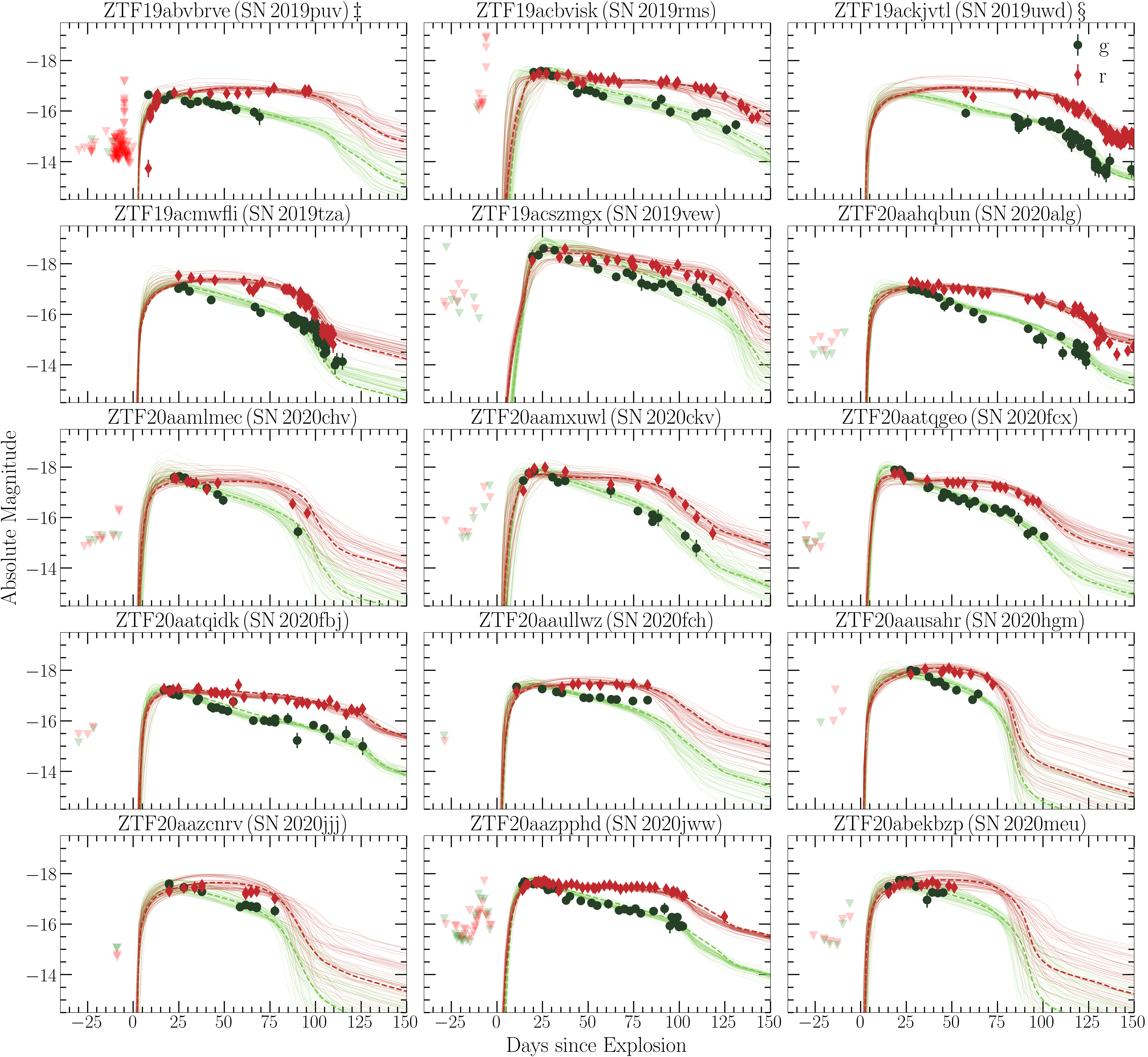
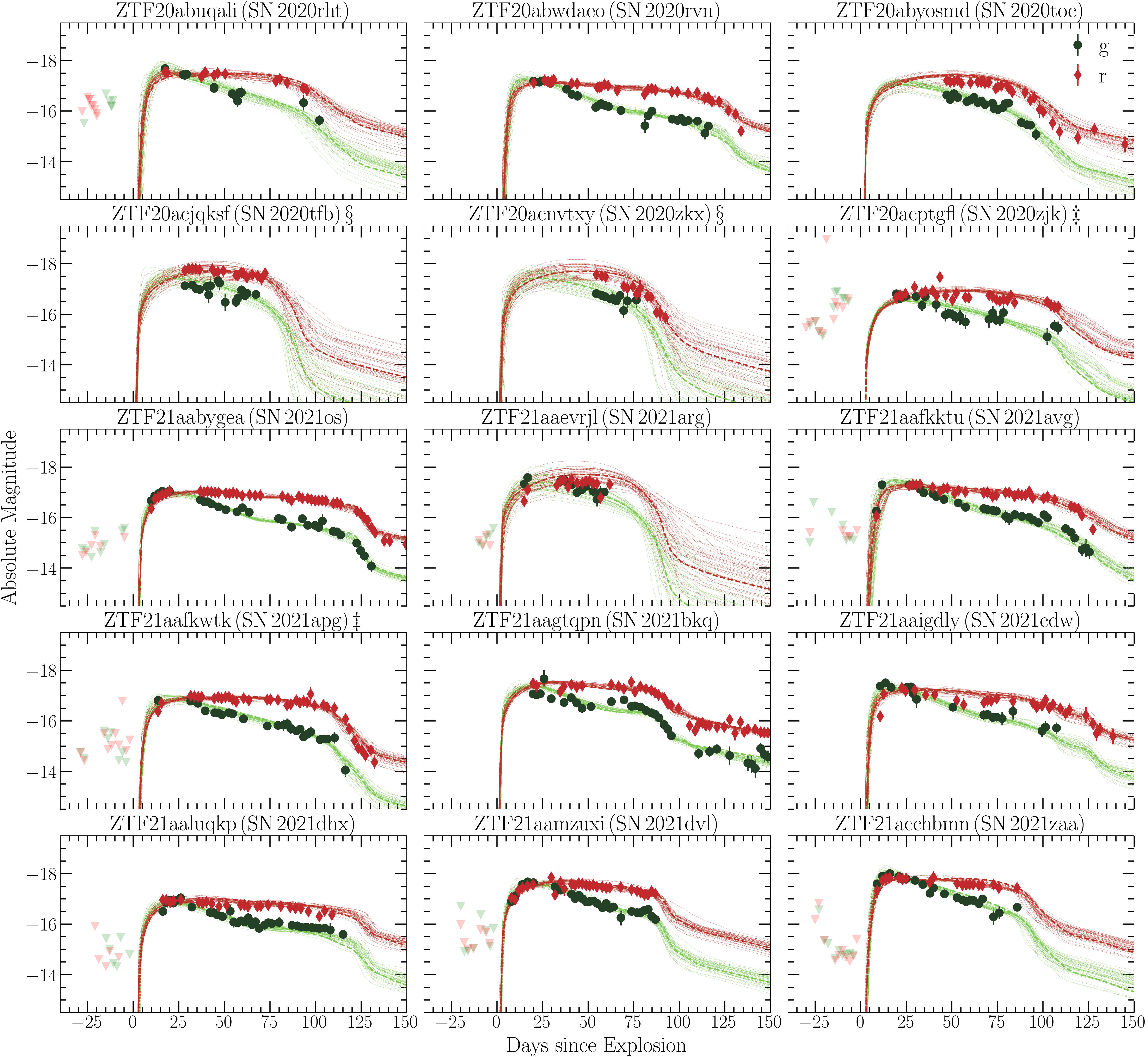
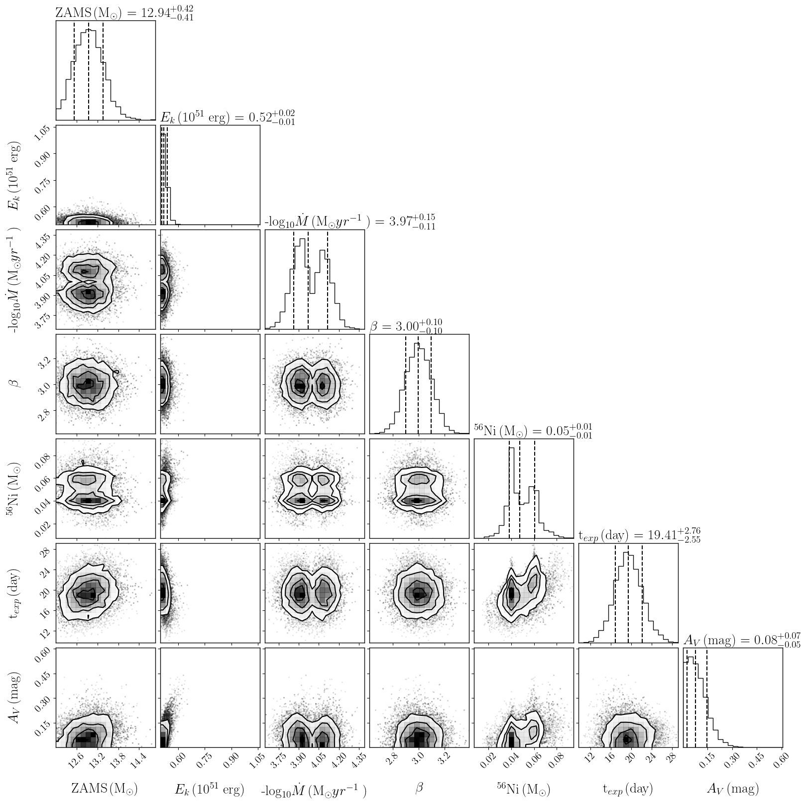
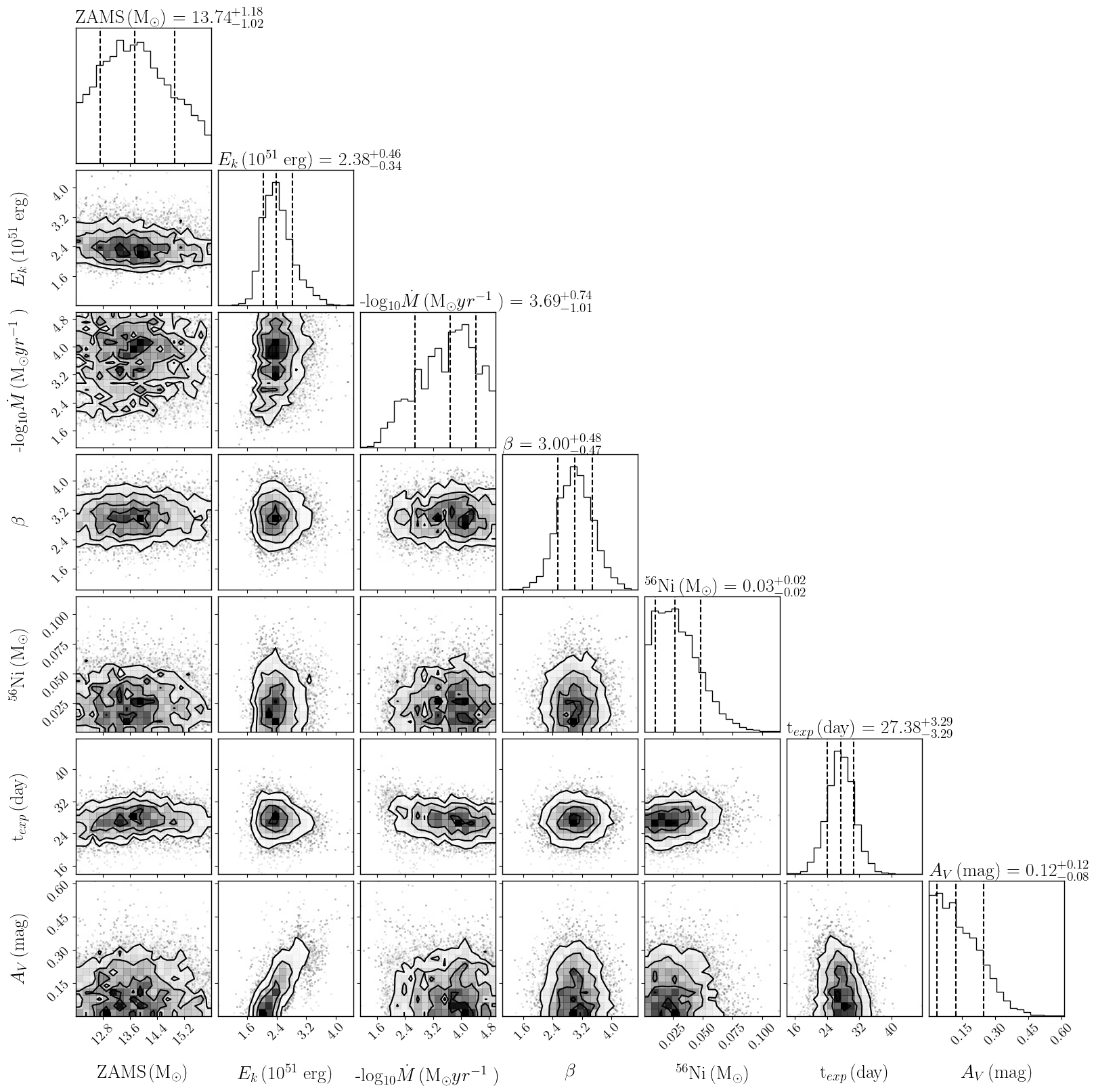
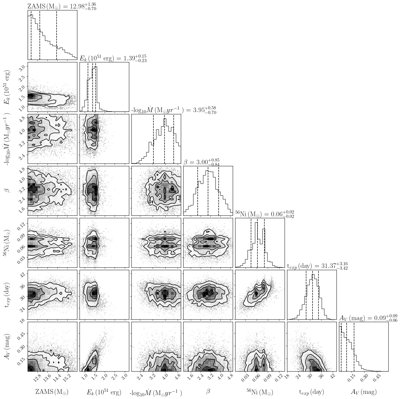
Using our Bayesian inference procedure to fit all ZTF events with our model grid, we derived the posterior probability distribution for all parameters of each Type II supernova. Our models were fit confidently to 34 events. The fits for the remaining 11 events were limited by poor upper limits prior to first detection (flagged with ) and the hydrodynamical model grid boundaries (flagged with ). Figure 1 shows the samples of the posterior probability distributions for the first 15 ZTF events. The light curve fits for the remaining events are plotted in an extended version of Figure 1 in Appendix. The observed data points are shifted with respect to the inferred explosion date and corrected for host extinction derived from the fits. The uncertainity in host extinction and explosion date is not represented in Figure 1. The dashed line in each passband represents the best fit model. Table 3 lists the inferred median values for the seven parameters with their 16th and 84th percentile confidence regions. We note that these uncertainities of the parameters only reflect how well the model fits the observed data and do not take into account any uncertainties related to the assumptions used to create the model grid itself. Representative corner plots of posterior probability distributions are shown in the Appendix.
ZTF21aabygea (SN 2021os) and ZTF18abcpmwh (SN 2018cur) yielded the highest ZAMS masses ( M⊙ and M⊙, respectively), while ZTF21aagtqpn (SN 2021bkq) has the lowest ( M⊙). The highest explosion energies are seen for ZTF18acuqskr (SN 2018jrb) and ZTF20aausahr (SN 2020hgm) ( erg and erg , respectively). Shown in Figure 1, these two events correspond to steeper and early declines in the light curves as compared to low energetic events ( erg ) including ZTF19ackjvtl (SN 2019uwd) and ZTF19acbvisk (SN 2019rms). These observed short-lived plateaus and fast declines are in agreement with previous results for other high energy CCSNe (Valenti et al., 2016; Rubin & Gal-Yam, 2017; de Jaeger et al., 2019; Barker et al., 2021). The more energetic events in our sample also show increased peak luminosity in both ztf– and ztf– bands (Galbany et al., 2016; Valenti et al., 2016; Sanders et al., 2015).
For seven events, our estimates of kinetic energy favor the minimum parameter value of our grid (0.5 erg). We flag these events as ones for which our model fits are less confident, since the actual kinetic energy may be significantly lower.
Most events (37 out of 45) in our sample tend to favor mass–loss rates between . However, a non-negligible number of events (8 out of 45) yield higher mass-loss rate estimates . This finding is consistent with Förster et al. (2018), who reported higher mass loss rates to be correlated with early and steep rises in the light curves of many Type II SNe from the High cadence Transient Survey (HiTS) (Förster et al., 2016), possibly due to shock-breakout in dense CSM (Moriya et al., 2011; Morozova et al., 2015; Moriya et al., 2017; Morozova et al., 2018; Moriya et al., 2018; Bruch et al., 2021; Haynie & Piro, 2021). We find that the fits for the steepness parameter are most likely prior dominated and favour values closer to , consistent with slowly accelerating winds found in red supergiants (Baade et al., 1996).
ZTF19abguqsi (SN 2019lsh) produced the least 56Ni mass of . Other ZTF events in the sample have estimates of 56Ni mass ranging from 0.02–0.1 . ZTF19aabvkly (SN 2019fmv), ZTF19abiahko (SN 2019lsj) and ZTF20aazcnrv (SN 2020jjj) have relatively short-lived plateau regions in their light curves and are associated with lower estimates of synthesized 56Ni mass (see Figure 1). Events with higher estimates of 56Ni mass have long–lived plateaus as compared to the the events with lower 56Ni mass estimates and faster declines in their light curves. These results are in agreement with previous analyses of SNe Type II that consider how 56Ni mass affects light curve evolution (Eastman et al., 1994; Bersten, 2013; Faran et al., 2014; Kozyreva et al., 2019).
ZTF20abyosmd (SN 2020toc) has the highest host extinction ( mag), followed by ZTF21aaevrjl (SN 2021arg) ( mag). ZTF18acbwasc (SN 2018hfc) and ZTF21aabygea (SN 2021os) have negligible host extinction values (both mag). All ZTF events in our sample show host extinction values ranging from mag, typical for CCSNe hosts (Pastorello et al., 2006; Maguire et al., 2010; Faran et al., 2014).
4.1 Correlations between physical parameters
We plot our inferred values with comparison to other similar works in literature (Förster et al., 2018; Martinez et al., 2020) in Figure 2. Förster et al. (2018) in their work uses hydrodynamical models on HiTS Type II supernovae that include estimates of circumstellar environment, while Martinez et al. (2020) do not include CSM structure in their models. Figure 2 shows the bounds of our model grid with grey dotted lines for each parameter in the plot. The ZTF events whose energy value fits approached the bounds of the model grid are marked in Table 3. We represent events that had relatively narrower prior distribution for explosion date inside the purple circle in Figure 2. These events had either constraining upper limits before first detection or enough rise time data to make an educated guess on the upper bound of prior distribution for explosion date.
Generally, our parameter estimates are less confident for ZTF events with poor data quality, such as those missing phases of light curves combined with unavailable upper limit constraints and whose parameter values approached the parameter boundaries of the model grid (see Table 3). These events are represented by green circles in Figure 2 as flagged events. Among 7 out of 11, ZTF18acbwasc (SN 2018hfc), ZTF19abhduuo (SN 2019lre), ZTF19abqyouo (SN 2019pbk), ZTF19ackjvtl (SN 2019uwd), ZTF20abyosmd (SN 2020toc), ZTF20acjqksf (SN 2020tfb) and ZTF20acnvtxy (SN 2020zkx) can be grouped together as events that have higher values for time of explosion ( 25 days). This could be attributed to the fact that the prior distribution was too broad as there were no upper limits for these events as provided by the ZTF survey. The remaining 4 ZTF events whose fits approached model boundaries are ZTF18acbvhit (SN 2018hle), ZTF19abvbrve (SN 2019puv), ZTF20acptgfl (SN 2020zjk), and ZTF21aafkwtk (SN 2021apg).
Moreover, we performed a Pearson correlation analysis to check if we can find any correlations between the physical parameters. However, we were unable to find any significant correlations (r or r ) within the sample studied. The correlation matrix is shown in Figure 3. The modest mass range in our model grid (12 - 16 M⊙) limits our ability to make strong claims on any potential ZAMS dependencies. For example, in Figure 2, the correlations in Martinez et al. (2020) becomes only clear when the ZAMS range is extended to 10 M⊙. Our hydrodynamical grid explores new parameter spaces that include mass-loss properties and this can possibly introduce additional degeneracies.
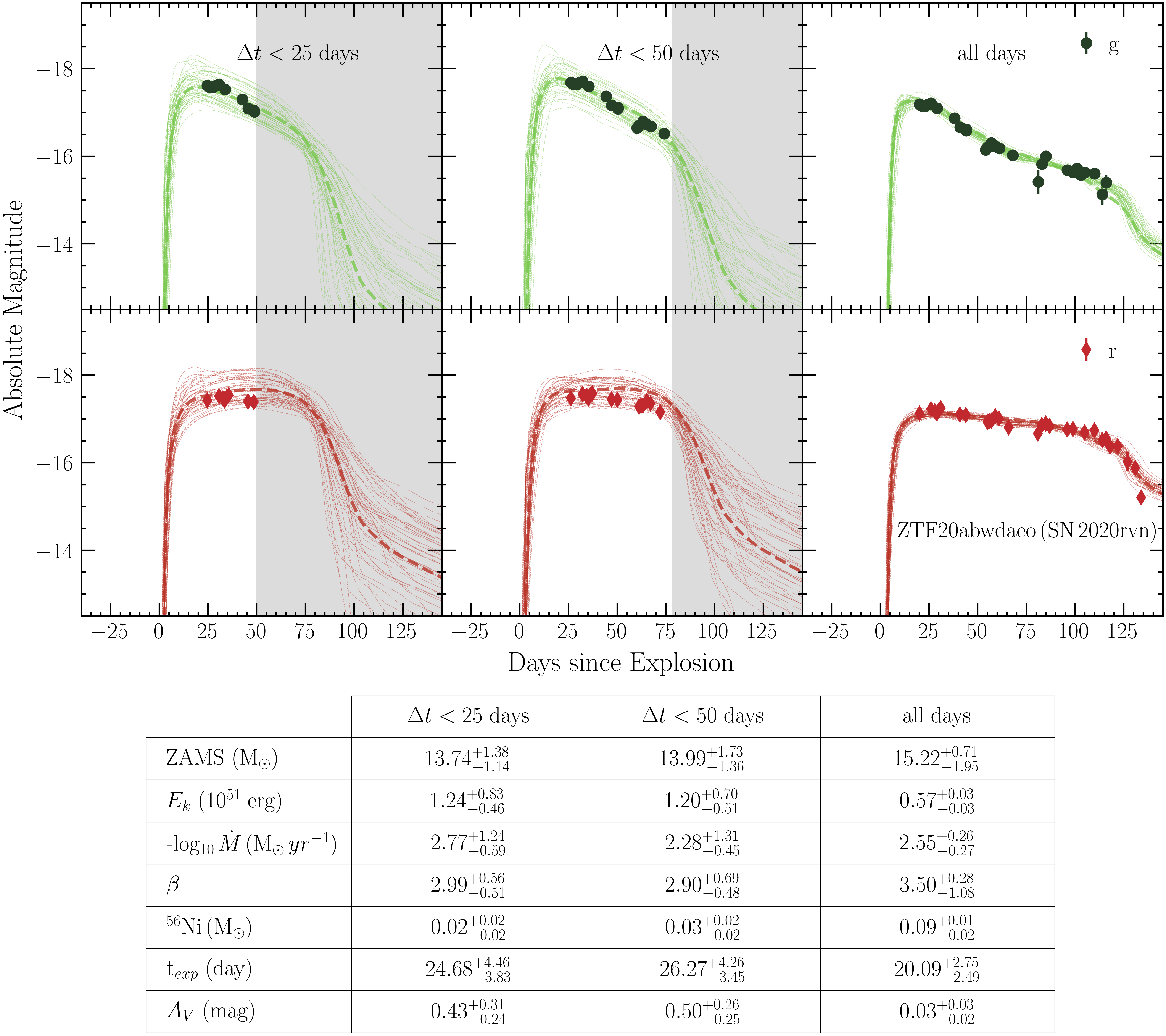
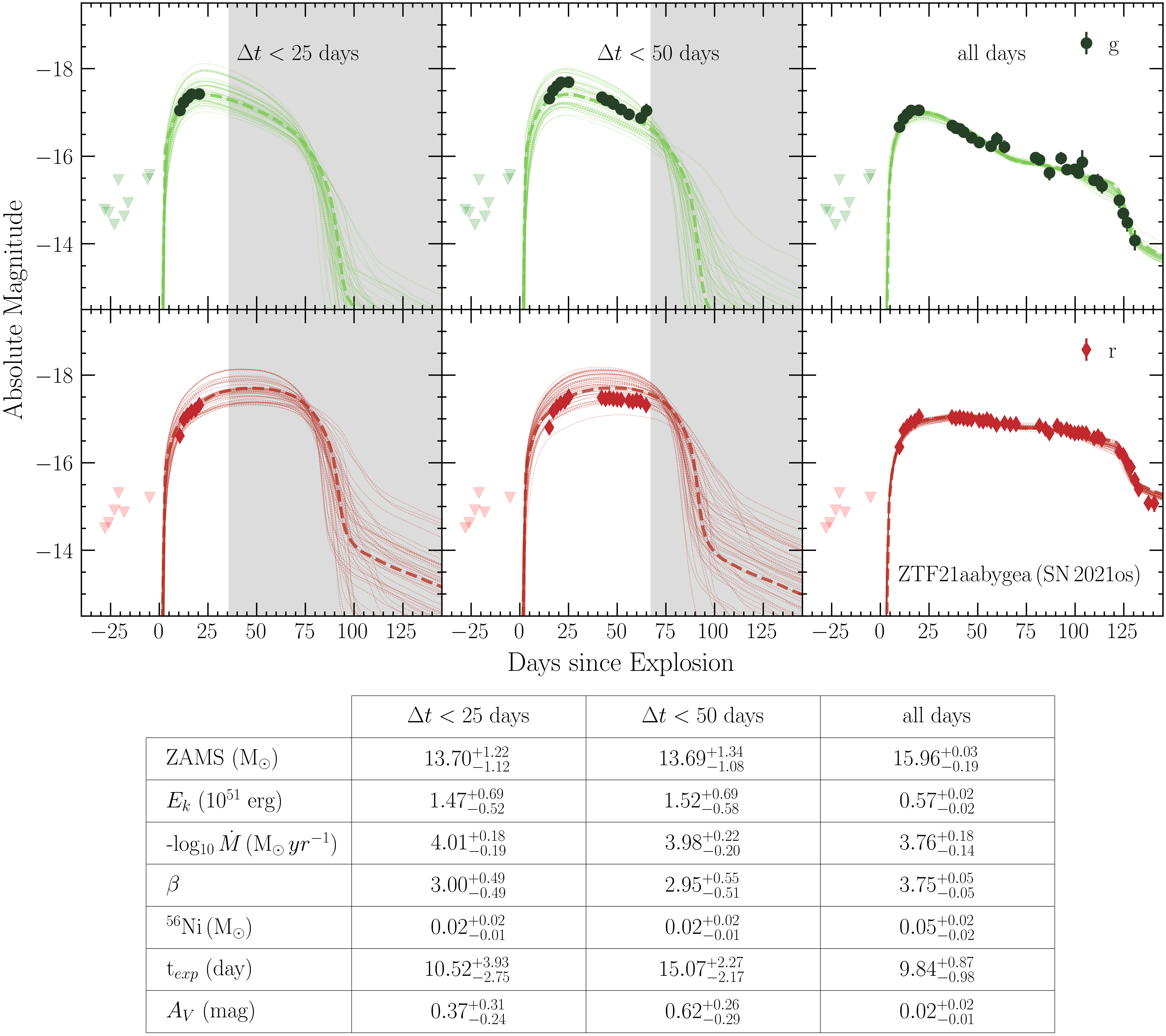
5 Real-time Parameter Evolution
We analyzed how each of the parameter fits evolved as a function of time, termed real-time characterization. We were motivated to characterize how well or poorly the model parameter fits and their uncertainties at fractional light curve stages anticipated the values found from complete light curves. We compared our model grid to three regimes of incomplete light curves with respect to the first detection: 1) days; 2) days; 3) all available data.
Figure 4 shows a detailed evolving characterization for the event ZTF19aaqdkrm (SN 2019dod). As expected, the fits and estimates of the parameters change with time as the supernova evolves and additional measurements are incorporated into the fitting process. Within days and days, the fits favor lower 56Ni masses and higher energies. As data in both bands accumulate, the fits favor higher 56Ni masses and lower energies. At days, the portion of the light curve powered by hydrogen recombination of the event starts to fall off, giving better estimates on ZAMS and 56Ni masses.
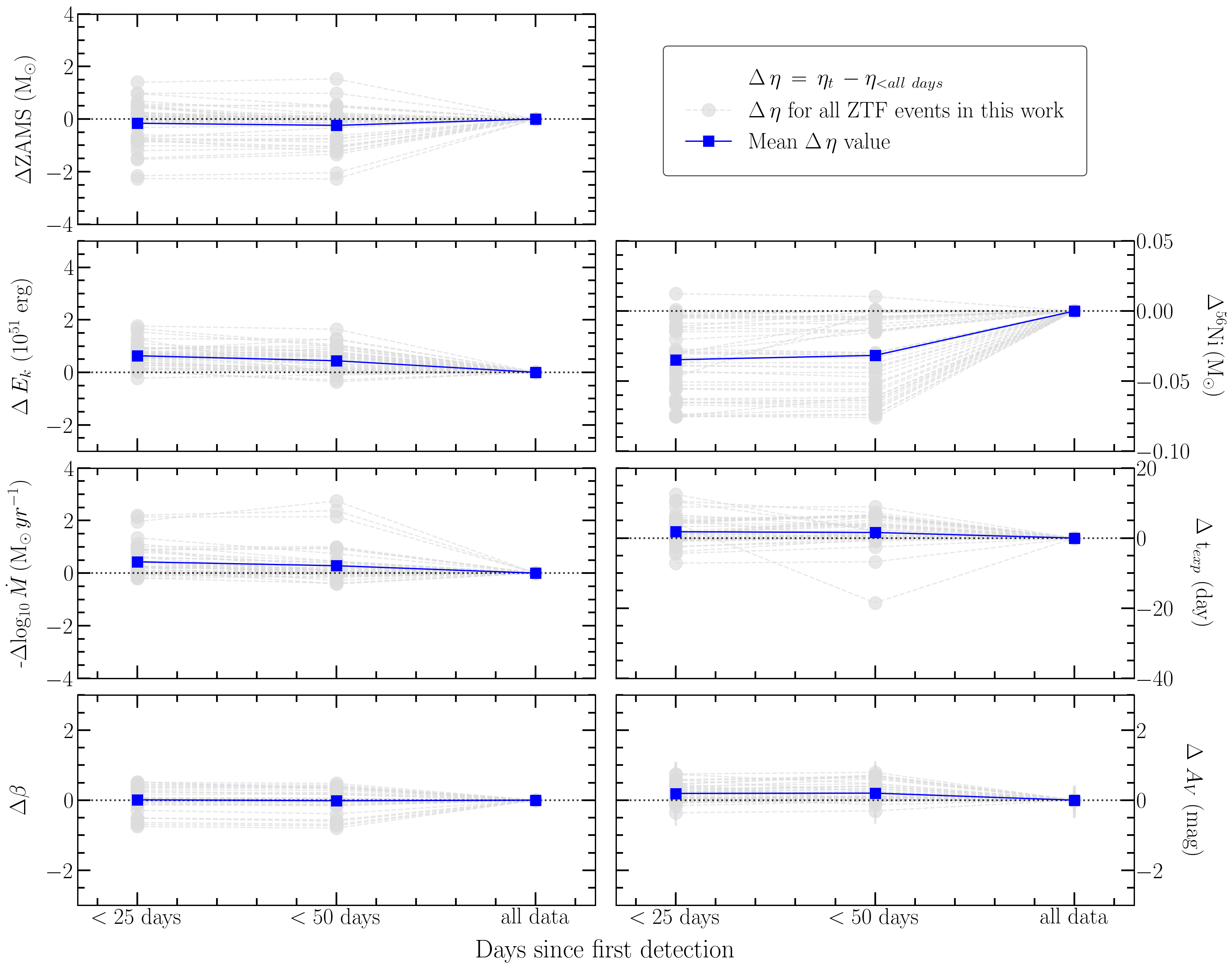
We performed this same analysis on all 45 ZTF events, where similar trends are seen. Figure 5 shows the difference in parameter values of our fits with respect to the final epoch with all the data as the event unfolds. Our analysis shows that the explosion energies and mass–loss rates for the events are initially overestimated and tend to favor lower final values when all data is included in the fit. This is opposite to what we see in case of 56Ni mass, as it is underestimated with only few measurements and consistently favors higher values for many events during later stages of light curve evolution as the recombination drop–off starts to unfold.
The most confident estimate of 56Ni mass is inferred when the hydrogen recombination phase ends and the radioactive decay phase starts. This results in epochs with all the data yielding higher estimates of 56Ni mass. With kinetic energy, the peak luminosity and decline rate of the light curve plays a significant role in estimating the energetics of the event. As a result, as more data become available at later epochs, more reliable estimates of kinetic energy are seen. The inferred values of ZAMS, host extinction, explosion date and the remain nearly constant as the light curve evolves.
6 Discussion
6.1 Parameter Space Degeneracy
A major challenge encountered when modelling only two passbands provided by public ZTF light curves was model degeneracy. Specifically, the probability that different combinations of explosion and progenitor parameters can potentially lead to the same light curve posed difficulties in converging to a unique solution in our fitting method. As noted in previous works, the hydrodynamical modelling approach has led to larger estimates of progenitor properties, especially ZAMS estimates, when compared to other approaches like pre-SN explosion imaging (Utrobin & Chugai, 2008, 2009; Maguire et al., 2010; Sanders et al., 2015). In the Appendix, posterior distribution of three ZTF events at various epochs are examined using kernel density estimation (KDE) analysis, along with a calculation of the number of modes. In a similar analysis for all 45 events, we find that all the ZTF events have multi-modal posteriors and temporal evolution of modes cannot be generalized.
Goldberg et al. (2019) recognize the challenges involved in breaking the degeneracies between ejecta mass, explosion energy and progenitor radius, and argue that in order to do so requires an independent measurement of one of the parameters. The scaling relationships used in their work yield families of explosions with varied parameters that can reproduce similar light curves. Hillier & Dessart (2019) also highlight calculations of similar photospheric phases for well-sampled Type II supernovae in their multi-band and spectroscopic modelling.
Martinez et al. (2020) attempt to partially lift this degeneracy issue by fitting photospheric velocity information from their models to velocity measurements obtained of SNe during the plateau phase. However, Goldberg et al. (2019) argue that only the ejecta velocities measured during the initial shock cooling phase can be useful to break these degeneracies seen in the parameters. Our analysis focused on photometry only, and future work can investigate whether use of kinematic information from spectroscopy can better constrain parameter selection.
6.2 Bolometric vs Pre-computed Multi-band Inference
Our analysis adopts the approach of fitting observations to synthetic multi-band photometry derived from theoretical hydrodynamical models. Similar works like Nicholl et al. (2017) and Guillochon et al. (2018) use semi-analytical, black body spectral energy distribution (SED) models to fit multi-band photometry for transients. These procedures contrast with typical methods that first construct bolometric light curves from multi-filter and/or multi–wavelength observations, that are in turn compared to model bolometric light curves. Each method has associated uncertainties. In the case of synthetic model photometry, uncertainties arise from assumptions in opacity treatment at different frequencies in STELLA. In the case of creating bolometric light curves from interpolated observed data sets, the uncertainties stem from potential gaps in photometry cadence, limited passbands, and potentially few data points overall to fit against.
For real time characterization of events, we found that a proper Bayesian inferencing of explosion parameters for large numbers of supernovae is most efficiently conducted with pre-computed grids of models. Computing models in real-time per event will lead to duplicative efforts and incur computational time costs. With our method, the fitting is more rapid, is more flexible, and the associated uncertainties are less significant.
6.3 Intelligent Augmentation
Our analysis only uses ZTF public data in ztf– and ztf– passbands to make inferences about Type II explosion parameters. Our parameter fits could be further constrained with observations at other passbands, and it is worthwhile to consider which passbands at which epochs are most constraining. To this end, inferencing transients in real time in order to make on-the-fly decisions about optimal follow-up in complementary passbands is needed (Carbone & Corsi, 2020; Sravan et al., 2021). Generally, most constraining for inferring Type II properties are observations at early and late phases of light curve evolution. At early phases, UV observations best sample shock breakout and circumstellar interaction (Gezari et al., 2015; Ganot et al., 2016; Soumagnac et al., 2020; Haynie & Piro, 2021; Jacobson-Galán et al., 2022). At late phases, near- and mid-infrared passbands provide diagnostics that best follow ejecta cooling and dust formation (Szalai & Vinkó, 2013; Bianco et al., 2014; Tinyanont et al., 2016). Optimally augmenting all-sky survey photometry in real-time in this way can enhance opportunities to generate large samples of core-collapse supernovae sufficiently observed to perform population and host-environment studies (D’Andrea et al., 2010; Anderson et al., 2014; Sanders et al., 2015; Schulze et al., 2021).
6.4 Anomaly Detection
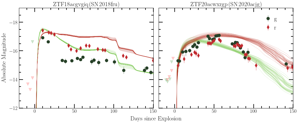
Our work uncovered two examples of anomalous Type II supernovae, which are not included in our sample of 45 events. We present the unusual light curves of ZTF18acgvgiq (SN 2018fru) and ZTF20acwxrgp (SN 2020acjg) in Figure 6. The fits for the entire light curves converged to a model solution with very poor likelihood scores resulting in inaccurate inferences. Consequently, we were unable to characterize these events with our current model grid. The anomalous nature of these events could be identified via poor model fits as early as days. The cumulative log-evidence (logZ) inferred for these two events were above -200 indicating very poor likelihood estimates when comparing the models with the data. For the events with good fits, the logZ estimates were under -20. These high logZ values indicate that the models were unable to converge to a target distribution of the parameters for the two anomalous events.
This experience shows that real-time inferencing can be used as a way to identify targets that deviate from normal theoretical predictions. Such real-time analyses for detecting anomalies (Pruzhinskaya et al., 2019; Soraisam et al., 2020; Villar et al., 2020; Ishida et al., 2021; Villar et al., 2021; Martínez-Galarza et al., 2021) can be automated into an ORACLE such as REFITT to motivate rapid spectroscopic follow–up of non-traditional CCSNe.
7 Conclusions
In this paper we have characterized 45 Type II supernovae using only products from the public ZTF survey (i.e., in ztf- and ztf- passbands) using a grid of theoretical hydrodynamical models. Our grid parameters span multiple supernova progenitor and explosion properties, as well as the time of explosion with respect to the first detection and host extinction. We compare results between complete and fractional light curves to determine which parameters are most robust to incomplete photometric data sets. This effort is to assess whether opportunities exist for theoretically-driven forecasts to inform when follow up observations are needed to support all-sky survey alert streams. The following conclusions are made:
-
•
We obtain confident characterizations for 34 SNe II in our sample. Inferences of the remaining 11 events are limited either by poorly constraining data or the boundaries of our model grid. The properties of these well-fitted events broadly follow those reported in previous analyses of SNe II.
-
•
In cases where fitted parameters derived from complete vs. incomplete data sets are compared, some parameters are more reliably determined at early epochs than others. The explosion energy, host extinction and mass-loss rate parameters are overestimated during initial phases of evolution, while the 56Ni mass is underestimated. The ZAMS mass and estimates do not change significantly at different phases.
-
•
The explosion date is a very sensitive parameter that requires well–constrained pre-explosion upper–limits from the survey for confident inferences. Generally, we found parameter estimates to be less reliable for ZTF events with poor data quality, such as missing phases of the light curve along with poor upper limit constraints.
-
•
Real-time Bayesian inferencing of progenitor and explosion parameters for large numbers of CCSNe from all-sky surveys demands a pre-computed grid of models. Creating synthetic model light curves in respective all-sky survey passbands catalyzes real-time characterization of evolving transients by avoiding challenges associated with constructing bolometric light curves with sparse and incomplete photometry.
Our work has demonstrated that hydrodynamical model grids for CCSNe along with statistical analyses can provide opportunities to enhance scientific return from all-sky surveys that provide live alert streams. Theoretically-driven predictions can be leveraged to efficiently coordinate worldwide observing facilities to conduct follow up observations that augment survey light curves to optimally achieve scientific objectives (Bianco et al., 2014; Modjaz et al., 2019; Kennamer et al., 2020; Sravan et al., 2020; Anand et al., 2021).
For example, real-time characterization can identify and prioritize transients that fall within certain parameter spaces of interest, including the extreme high and low ends of kinetic energy or 56Ni mass. Likewise, theoretical forecasts can identify and prioritize follow up photometry at critical phases of transient evolution, including monitoring the plateau drop-off of SNe II light curves that provides information needed to improve estimates of kinetic energy and ZAMS and 56Ni masses. Ideally, predicting transient evolution using the underlying physics of transients can be incorporated into a TOM or ORACLE that can efficiently recommend targets for follow-up at information-rich epochs (Djorgovski et al., 2016; Street et al., 2018; Kasliwal et al., 2019; Sravan et al., 2020; Agayeva et al., 2021).
Our future work relies on an expanded grid of hydrodynamical models exploring larger parameter ranges, including varying degrees of 56Ni mixing within the inner layers of the progenitors, and information on photospheric velocity that can be used to potentially break degeneracies between parameters. It will also expand synthetic photometry to all six passbands of LSST. Although our work focuses on Type II CCSNe, our methods can be easily applied to identify, prioritize and coordinate follow-up of other transients discovered by Vera C. Rubin Observatory.
Acknowledgements
The authors would like to thank the anonymous referee for helpful comments that have significantly improved this paper. We also acknowledge helpful discussions with Thomas Matheson, Mariana Orellana, and Melina Bersten. The ZTF forced-photometry service was funded under the Heising-Simons Foundation grant #12540303 (PI: Graham). Numerical computations were in part carried out on PC cluster at Center for Computational Astrophysics (CfCA), National Astronomical Observatory of Japan. D. M. acknowledges NSF support from grants PHY-1914448, PHY- 2209451, AST-2037297, and AST-2206532.
Appendix A Multi-epoch Evolution of Posterior Distribution of Parameters
We performed a kernel density estimation (KDE) analysis in order to find the modality of the posterior distributions at various epochs. The samples in the posterior distribution were collected and smoothed using Silverman’s bandwidth with a gaussian kernel. The KDE approximated distribution was then used to calculate the number of modes at every epoch. The modes were found by identifying inflection points in the distribution i.e positions where the first derivative changes the sign.
We found that all the objects have multi-modal posteriors for at least one parameter in our analysis. From this analysis, we conclude that the change in the posteriors for physical parameters over different epochs cannot be generalized for all the events. Figure 14 shows examples of multi-modal posteriors for ZAMS, Kinetic Energy and 56Ni for three ZTF events The red circles represent different modes found in the distribution using inflection point analysis. We note that the modes of the distribution for kinetic energy shift from higher to lower values as time proceeds in Figure 14 for each event as discussed in the paper. The trend in 56Ni with time is reflected in the modes with earlier epochs favouring lower values as compared with final epochs. The degeneracies in parameter space as discussed in 6.1 are clearly reflected in these distributions through multi-modality.
References
- Agayeva et al. (2021) Agayeva, S., Alishov, S., Antier, S., et al. 2021, in Revista Mexicana de Astronomia y Astrofisica Conference Series, Vol. 53, Revista Mexicana de Astronomia y Astrofisica Conference Series, 198–205, doi: 10.22201/ia.14052059p.2021.53.39
- Alves et al. (2022) Alves, C. S., Peiris, H. V., Lochner, M., et al. 2022, ApJS, 258, 23, doi: 10.3847/1538-4365/ac3479
- Anand et al. (2021) Anand, S., Coughlin, M. W., Kasliwal, M. M., et al. 2021, Nature Astronomy, 5, 46, doi: 10.1038/s41550-020-1183-3
- Anderson et al. (2014) Anderson, J. P., González-Gaitán, S., Hamuy, M., et al. 2014, ApJ, 786, 67, doi: 10.1088/0004-637X/786/1/67
- Astropy Collaboration et al. (2013) Astropy Collaboration, Robitaille, T. P., Tollerud, E. J., et al. 2013, A&A, 558, A33, doi: 10.1051/0004-6361/201322068
- Astropy Collaboration et al. (2018) Astropy Collaboration, Price-Whelan, A. M., Sipőcz, B. M., et al. 2018, AJ, 156, 123, doi: 10.3847/1538-3881/aabc4f
- Baade et al. (1996) Baade, R., Kirsch, T., Reimers, D., et al. 1996, ApJ, 466, 979, doi: 10.1086/177569
- Barker et al. (2021) Barker, B. L., Harris, C. E., Warren, M. L., O’Connor, E. P., & Couch, S. M. 2021, arXiv e-prints, arXiv:2102.01118. https://arxiv.org/abs/2102.01118
- Bellm et al. (2019) Bellm, E. C., Kulkarni, S. R., Graham, M. J., et al. 2019, PASP, 131, 018002, doi: 10.1088/1538-3873/aaecbe
- Bersten (2013) Bersten, M. C. 2013, arXiv e-prints, arXiv:1303.0639. https://arxiv.org/abs/1303.0639
- Bianco et al. (2014) Bianco, F. B., Modjaz, M., Hicken, M., et al. 2014, ApJS, 213, 19, doi: 10.1088/0067-0049/213/2/19
- Blinnikov et al. (2000) Blinnikov, S., Lundqvist, P., Bartunov, O., Nomoto, K., & Iwamoto, K. 2000, ApJ, 532, 1132, doi: 10.1086/308588
- Blinnikov et al. (1998) Blinnikov, S. I., Eastman, R., Bartunov, O. S., Popolitov, V. A., & Woosley, S. E. 1998, ApJ, 496, 454, doi: 10.1086/305375
- Blinnikov et al. (2006) Blinnikov, S. I., Röpke, F. K., Sorokina, E. I., et al. 2006, A&A, 453, 229, doi: 10.1051/0004-6361:20054594
- Borne (2008) Borne, K. D. 2008, Astronomische Nachrichten, 329, 255, doi: 10.1002/asna.200710946
- Bruch et al. (2021) Bruch, R. J., Gal-Yam, A., Schulze, S., et al. 2021, ApJ, 912, 46, doi: 10.3847/1538-4357/abef05
- Carbone & Corsi (2020) Carbone, D., & Corsi, A. 2020, ApJ, 889, 36, doi: 10.3847/1538-4357/ab6227
- D’Andrea et al. (2010) D’Andrea, C. B., Sako, M., Dilday, B., et al. 2010, ApJ, 708, 661, doi: 10.1088/0004-637X/708/1/661
- de Jaeger et al. (2019) de Jaeger, T., Zheng, W., Stahl, B. E., et al. 2019, MNRAS, 490, 2799, doi: 10.1093/mnras/stz2714
- Djorgovski et al. (2016) Djorgovski, S. G., Graham, M. J., Donalek, C., et al. 2016, arXiv e-prints, arXiv:1601.04385. https://arxiv.org/abs/1601.04385
- Eastman et al. (1994) Eastman, R. G., Woosley, S. E., Weaver, T. A., & Pinto, P. A. 1994, ApJ, 430, 300, doi: 10.1086/174404
- Faran et al. (2014) Faran, T., Poznanski, D., Filippenko, A. V., et al. 2014, MNRAS, 442, 844, doi: 10.1093/mnras/stu955
- Förster et al. (2016) Förster, F., Maureira, J. C., San Martín, J., et al. 2016, ApJ, 832, 155, doi: 10.3847/0004-637X/832/2/155
- Förster et al. (2018) Förster, F., Moriya, T. J., Maureira, J. C., et al. 2018, Nature Astronomy, 2, 808, doi: 10.1038/s41550-018-0563-4
- Förster et al. (2021) Förster, F., Cabrera-Vives, G., Castillo-Navarrete, E., et al. 2021, AJ, 161, 242, doi: 10.3847/1538-3881/abe9bc
- Gal-Yam (2021) Gal-Yam, A. 2021, in American Astronomical Society Meeting Abstracts, Vol. 53, American Astronomical Society Meeting Abstracts, 423.05
- Galbany et al. (2016) Galbany, L., Hamuy, M., Phillips, M. M., et al. 2016, The Astronomical Journal, 151, 33, doi: 10.3847/0004-6256/151/2/33
- Ganot et al. (2016) Ganot, N., Gal-Yam, A., Ofek, E. O., et al. 2016, ApJ, 820, 57, doi: 10.3847/0004-637X/820/1/57
- García-Jara et al. (2022) García-Jara, G., Protopapas, P., & Estévez, P. A. 2022, arXiv e-prints, arXiv:2205.06758. https://arxiv.org/abs/2205.06758
- Garretson et al. (2021) Garretson, B., Milisavljevic, D., Reynolds, J., et al. 2021, Research Notes of the American Astronomical Society, 5, 283, doi: 10.3847/2515-5172/ac416e
- Gezari et al. (2015) Gezari, S., Jones, D. O., Sanders, N. E., et al. 2015, ApJ, 804, 28, doi: 10.1088/0004-637X/804/1/28
- Goldberg et al. (2019) Goldberg, J. A., Bildsten, L., & Paxton, B. 2019, ApJ, 879, 3, doi: 10.3847/1538-4357/ab22b6
- Guillochon et al. (2018) Guillochon, J., Nicholl, M., Villar, V. A., et al. 2018, ApJS, 236, 6, doi: 10.3847/1538-4365/aab761
- Haynie & Piro (2021) Haynie, A., & Piro, A. L. 2021, ApJ, 910, 128, doi: 10.3847/1538-4357/abe938
- Hillier & Dessart (2019) Hillier, D. J., & Dessart, L. 2019, A&A, 631, A8, doi: 10.1051/0004-6361/201935100
- Huerta et al. (2019) Huerta, E. A., Allen, G., Andreoni, I., et al. 2019, Nature Reviews Physics, 1, 600, doi: 10.1038/s42254-019-0097-4
- IRSA (2022) IRSA. 2022, Zwicky Transient Facility Image Service, IPAC, doi: 10.26131/IRSA539
- Ishida et al. (2021) Ishida, E. E. O., Kornilov, M. V., Malanchev, K. L., et al. 2021, A&A, 650, A195, doi: 10.1051/0004-6361/202037709
- Ivezić et al. (2019) Ivezić, Ž., Kahn, S. M., Tyson, J. A., et al. 2019, ApJ, 873, 111, doi: 10.3847/1538-4357/ab042c
- Jacobson-Galán et al. (2022) Jacobson-Galán, W. V., Dessart, L., Jones, D. O., et al. 2022, ApJ, 924, 15, doi: 10.3847/1538-4357/ac3f3a
- Kasen & Woosley (2009) Kasen, D., & Woosley, S. E. 2009, ApJ, 703, 2205, doi: 10.1088/0004-637X/703/2/2205
- Kasliwal et al. (2019) Kasliwal, M. M., Cannella, C., Bagdasaryan, A., et al. 2019, PASP, 131, 038003, doi: 10.1088/1538-3873/aafbc2
- Kennamer et al. (2020) Kennamer, N., Ishida, E. E. O., Gonzalez-Gaitan, S., et al. 2020, arXiv e-prints, arXiv:2010.05941. https://arxiv.org/abs/2010.05941
- Kochanek et al. (2012) Kochanek, C. S., Khan, R., & Dai, X. 2012, ApJ, 759, 20, doi: 10.1088/0004-637X/759/1/20
- Kozyreva et al. (2019) Kozyreva, A., Nakar, E., & Waldman, R. 2019, MNRAS, 483, 1211, doi: 10.1093/mnras/sty3185
- LSST Science Collaboration et al. (2009) LSST Science Collaboration, Abell, P. A., Allison, J., et al. 2009, arXiv e-prints, arXiv:0912.0201. https://arxiv.org/abs/0912.0201
- LSST Science Collaboration et al. (2017) LSST Science Collaboration, Marshall, P., Anguita, T., et al. 2017, arXiv e-prints, arXiv:1708.04058. https://arxiv.org/abs/1708.04058
- Maguire et al. (2010) Maguire, K., Di Carlo, E., Smartt, S. J., et al. 2010, MNRAS, 404, 981, doi: 10.1111/j.1365-2966.2010.16332.x
- Martinez et al. (2020) Martinez, L., Bersten, M. C., Anderson, J. P., et al. 2020, A&A, 642, A143, doi: 10.1051/0004-6361/202038393
- Martínez-Galarza et al. (2021) Martínez-Galarza, J. R., Bianco, F. B., Crake, D., et al. 2021, MNRAS, 508, 5734, doi: 10.1093/mnras/stab2588
- Masci et al. (2019) Masci, F. J., Laher, R. R., Rusholme, B., et al. 2019, PASP, 131, 018003, doi: 10.1088/1538-3873/aae8ac
- Matheson et al. (2021) Matheson, T., Stubens, C., Wolf, N., et al. 2021, AJ, 161, 107, doi: 10.3847/1538-3881/abd703
- Mattila et al. (2012) Mattila, S., Dahlen, T., Efstathiou, A., et al. 2012, ApJ, 756, 111, doi: 10.1088/0004-637X/756/2/111
- Mauron & Josselin (2011) Mauron, N., & Josselin, E. 2011, A&A, 526, A156, doi: 10.1051/0004-6361/201013993
- Modjaz et al. (2019) Modjaz, M., Gutiérrez, C. P., & Arcavi, I. 2019, Nature Astronomy, 3, 717, doi: 10.1038/s41550-019-0856-2
- Möller & de Boissière (2020) Möller, A., & de Boissière, T. 2020, MNRAS, 491, 4277, doi: 10.1093/mnras/stz3312
- Möller et al. (2021) Möller, A., Peloton, J., Ishida, E. E. O., et al. 2021, MNRAS, 501, 3272, doi: 10.1093/mnras/staa3602
- Moriya et al. (2011) Moriya, T., Tominaga, N., Blinnikov, S. I., Baklanov, P. V., & Sorokina, E. I. 2011, MNRAS, 415, 199, doi: 10.1111/j.1365-2966.2011.18689.x
- Moriya et al. (2018) Moriya, T. J., Förster, F., Yoon, S.-C., Gräfener, G., & Blinnikov, S. I. 2018, MNRAS, 476, 2840, doi: 10.1093/mnras/sty475
- Moriya et al. (2017) Moriya, T. J., Yoon, S.-C., Gräfener, G., & Blinnikov, S. I. 2017, MNRAS, 469, L108, doi: 10.1093/mnrasl/slx056
- Morozova et al. (2015) Morozova, V., Piro, A. L., Renzo, M., et al. 2015, ApJ, 814, 63, doi: 10.1088/0004-637X/814/1/63
- Morozova et al. (2018) Morozova, V., Piro, A. L., & Valenti, S. 2018, ApJ, 858, 15, doi: 10.3847/1538-4357/aab9a6
- Najita et al. (2016) Najita, J., Willman, B., Finkbeiner, D. P., et al. 2016, arXiv e-prints, arXiv:1610.01661. https://arxiv.org/abs/1610.01661
- Narayan et al. (2018) Narayan, G., Zaidi, T., Soraisam, M. D., et al. 2018, ApJS, 236, 9, doi: 10.3847/1538-4365/aab781
- Nicholl et al. (2017) Nicholl, M., Guillochon, J., & Berger, E. 2017, ApJ, 850, 55, doi: 10.3847/1538-4357/aa9334
- Pastorello et al. (2006) Pastorello, A., Sauer, D., Taubenberger, S., et al. 2006, MNRAS, 370, 1752, doi: 10.1111/j.1365-2966.2006.10587.x
- Pruzhinskaya et al. (2019) Pruzhinskaya, M. V., Malanchev, K. L., Kornilov, M. V., et al. 2019, MNRAS, 489, 3591, doi: 10.1093/mnras/stz2362
- Ricks & Dwarkadas (2019) Ricks, W., & Dwarkadas, V. V. 2019, arXiv e-prints, arXiv:1906.07311. https://arxiv.org/abs/1906.07311
- Rubin & Gal-Yam (2017) Rubin, A., & Gal-Yam, A. 2017, ApJ, 848, 8, doi: 10.3847/1538-4357/aa8465
- Sánchez-Sáez et al. (2021) Sánchez-Sáez, P., Reyes, I., Valenzuela, C., et al. 2021, AJ, 161, 141, doi: 10.3847/1538-3881/abd5c1
- Sanders et al. (2015) Sanders, N. E., Soderberg, A. M., Gezari, S., et al. 2015, ApJ, 799, 208, doi: 10.1088/0004-637X/799/2/208
- Schlegel et al. (1998) Schlegel, D. J., Finkbeiner, D. P., & Davis, M. 1998, ApJ, 500, 525, doi: 10.1086/305772
- Schulze et al. (2021) Schulze, S., Yaron, O., Sollerman, J., et al. 2021, ApJS, 255, 29, doi: 10.3847/1538-4365/abff5e
- Shappee et al. (2014) Shappee, B. J., Prieto, J. L., Grupe, D., et al. 2014, ApJ, 788, 48, doi: 10.1088/0004-637X/788/1/48
- Skilling (2004) Skilling, J. 2004, in American Institute of Physics Conference Series, Vol. 735, Bayesian Inference and Maximum Entropy Methods in Science and Engineering: 24th International Workshop on Bayesian Inference and Maximum Entropy Methods in Science and Engineering, ed. R. Fischer, R. Preuss, & U. V. Toussaint, 395–405, doi: 10.1063/1.1835238
- Skilling (2006) Skilling, J. 2006, Bayesian Analysis, 1, 833 , doi: 10.1214/06-BA127
- Smith (2019) Smith, K. 2019, in The Extragalactic Explosive Universe: the New Era of Transient Surveys and Data-Driven Discovery, 51, doi: 10.5281/zenodo.3478098
- Sooknunan et al. (2021) Sooknunan, K., Lochner, M., Bassett, B. A., et al. 2021, MNRAS, 502, 206, doi: 10.1093/mnras/staa3873
- Soraisam et al. (2020) Soraisam, M. D., Saha, A., Matheson, T., et al. 2020, ApJ, 892, 112, doi: 10.3847/1538-4357/ab7b61
- Soumagnac et al. (2020) Soumagnac, M. T., Ofek, E. O., Liang, J., et al. 2020, ApJ, 899, 51, doi: 10.3847/1538-4357/ab94be
- Sravan et al. (2021) Sravan, N., Graham, M. J., Fremling, C., & Coughlin, M. W. 2021, arXiv e-prints, arXiv:2112.05897. https://arxiv.org/abs/2112.05897
- Sravan et al. (2020) Sravan, N., Milisavljevic, D., Reynolds, J. M., Lentner, G., & Linvill, M. 2020, ApJ, 893, 127, doi: 10.3847/1538-4357/ab8128
- Street et al. (2018) Street, R. A., Bowman, M., Saunders, E. S., & Boroson, T. 2018, in Society of Photo-Optical Instrumentation Engineers (SPIE) Conference Series, Vol. 10707, Software and Cyberinfrastructure for Astronomy V, ed. J. C. Guzman & J. Ibsen, 1070711, doi: 10.1117/12.2312293
- Sukhbold et al. (2016) Sukhbold, T., Ertl, T., Woosley, S. E., Brown, J. M., & Janka, H. T. 2016, ApJ, 821, 38, doi: 10.3847/0004-637X/821/1/38
- Szalai & Vinkó (2013) Szalai, T., & Vinkó, J. 2013, A&A, 549, A79, doi: 10.1051/0004-6361/201220015
- Tinyanont et al. (2016) Tinyanont, S., Kasliwal, M. M., Fox, O. D., et al. 2016, ApJ, 833, 231, doi: 10.3847/1538-4357/833/2/231
- Tonry et al. (2018) Tonry, J. L., Denneau, L., Heinze, A. N., et al. 2018, PASP, 130, 064505, doi: 10.1088/1538-3873/aabadf
- Utrobin & Chugai (2008) Utrobin, V. P., & Chugai, N. N. 2008, A&A, 491, 507, doi: 10.1051/0004-6361:200810272
- Utrobin & Chugai (2009) —. 2009, A&A, 506, 829, doi: 10.1051/0004-6361/200912273
- Valenti et al. (2016) Valenti, S., Howell, D. A., Stritzinger, M. D., et al. 2016, MNRAS, 459, 3939, doi: 10.1093/mnras/stw870
- Villar et al. (2021) Villar, V. A., Cranmer, M., Berger, E., et al. 2021, ApJS, 255, 24, doi: 10.3847/1538-4365/ac0893
- Villar et al. (2020) Villar, V. A., Cranmer, M., Contardo, G., Ho, S., & Yao-Yu Lin, J. 2020, arXiv e-prints, arXiv:2010.11194. https://arxiv.org/abs/2010.11194
- Weaver et al. (1978) Weaver, T. A., Zimmerman, G. B., & Woosley, S. E. 1978, ApJ, 225, 1021, doi: 10.1086/156569
- Woosley et al. (2002) Woosley, S. E., Heger, A., & Weaver, T. A. 2002, Reviews of Modern Physics, 74, 1015, doi: 10.1103/RevModPhys.74.1015