Quantum Gravitational Sensor for Space Debris

Abstract

Matter-wave interferometers have fundamental applications for gravity experiments such as testing the equivalence principle and the quantum nature of gravity. In addition, matter-wave interferometers can be used as quantum sensors to measure the local gravitational acceleration caused by external massive moving objects, thus lending itself for technological applications. In this paper, we will establish a three dimensional model to describe the gravity gradient signal from an external moving object, and theoretically investigate the achievable sensitivities using the matter-wave interferometer based on the Stern-Gerlach set-up. As an application we will consider the Mesoscopic Interference for Metric and Curvature (MIMAC) and Gravitational wave detection scheme [New J. Phys. 22, 083012 (2020)] and quantify its sensitivity to gravity gradients using frequency-space analysis. We will consider objects near Earth-based experiments and space debris in proximity of satellites and estimate the minimum detectable mass of the object as a function of their distance, velocity, and orientation.

I Introduction

Interferometry has many salient applications Bongs_2004 in gravity experiments such as testing the equivalence principle PhysRevLett.120.183604 ; PhysRevLett.125.191101 ; Bose:2022czr and measuring the Earth’s gravitational acceleration Peters1999 ; Marshman:2018upe ; Chiao:2003sa ; Roura:2004se ; Foffa:2004up ; Dimopoulos:2008sv ; Dimopoulos:2007cj ; Tino:2019tkb ; Asenbaum:2020era ; Graham:2012sy . The seminal works on neutron interferometry PhysRevLett.34.1472 ; werner1979effect ; 9780198712510.001.0001 motivated a series of matter-wave interferometers Nesvizhevsky2002 ; science.1135459 ; asenbaum2017phase ; overstreet2022observation as well as led to more recent developments in photon interferometry Bertocchi_2006 ; Fink2017 ; PhysRevLett.123.110401 ; torovs2020revealing ; cromb2022controlling ; torovs2022generation .

One of the latest quests is to build a matter-wave interferometer with nanoparticles to test the quantum nature of gravity in a laboratory PhysRevLett.119.240401 ; ICTS (for a related work see PhysRevLett.119.240402 ). The scheme relies on two masses, each prepared in a spatial superposition, and placed at distances where they couple gravitationally, but still sufficiently far apart that all other interactions remain suppressed. If gravity is a bonafide quantum entity, and not a classical real-valued field, then the two masses will entangle Marshman:2019sne ; Bose:2022uxe ; Christodoulou:2022vte ; Danielson:2021egj . To test the quantum nature of gravity we will need particles of mass $\sim 10^{-14}-10^{-15}$ kg, an interferometric scheme for preparing large superposition sizes $\sim 100\,\rm\mu m$, and exquisite experimental control to guarantee coherence times of $\sim 1$ s PhysRevLett.119.240401 ; Pino_2018 ; PhysRevA.102.062807 ; Toros:2020dbf ; Tilly:2021qef ; Schut:2021svd ; Nguyen2020 ; PhysRevA.102.022428 .

One of the most promising approaches towards interferometry with nanoparticles is based on the Stern-Gerlach (SG) apparatus friedrich2021molecular . SG interferometers have been already experimentally realized using an atom chip Keil2021 , with the half-loop Machluf2013 and full-loop SGI_experiment configurations achieving the superposition size of 3.93 $\rm\mu m$ and $0.38\,\rm\mu m$ in the experimental time of 21.45 ms and 7 ms, respectively SGI_experiment . This basic SG scheme can be adapted to the mass range of nanoparticles using nanodiamond like materials with embedded nitrogen vacancy (NV) centers. Such a system has an internal spin degree of freedom and can thus be placed in a large spatial superposition using the SG setup PhysRevLett.119.240401 ; Marshman:2021wyk ; Zhou:2022frl ; Zhou:2022jug ; Zhou:2022epb .

One of the main challenges of nanocrystal matter-wave interferometry is to tame the numerous decoherence and noise sources. Common sources for the loss of visibility, such as the ones arising from residual gas collisions and environmental photons, can be attenuated by vacuum and low-temperature technologies Pino_2018 ; PhysRevA.102.062807 ; Toros:2020dbf ; Tilly:2021qef ; Schut:2021svd ; Nguyen2020 ; PhysRevA.102.022428 . In addition, the spin decoherence should also been taken into account, i.e., the Humpty-Dumpty effect Englert1988 ; Schwinger1988 ; PMID:9902333 ; Zhou:2022frl ; Japha:2022xyg , with methods to extend the spin coherence time, as well as tackle the Majorana spin-flip, under development Inguscio:2007xi ; Marshman:2021wyk ; Zhou:2022frl . Moreover, there are also a series of gravitational channels for decoherence; the emission of gravitons is negligible torovs2020loss , decoherence induced by the gravitational interaction with the experimental apparatus can be reduced using a hierarchy of distances Gunnink:2022ner , and gravity gradient noise (GGN) can be mitigated with an exclusion zone Toros:2020dbf . GGN is equally important for the gravitational wave observatories Harms2019 ; PhysRevD.103.103017 such as LIGO PhysRevD.58.122002 ; PhysRevD.60.082001 ; PhysRevD.98.083019 , Virgo Beccaria:1998ap ; Acernese_2014 , KAGRA KAGRA , LISA Lisa406065 ; PhysRevD.70.063512 ; PhysRevD.106.063015 ; Adams:2004pk and Einstein TelescopeBader_2022 , in particular at the low frequencies.

In this work, we will investigate the possibility of using the nanoparticle matter-wave interferometer as a gravity gradient quantum sensor. We will estimate the required sensitivities to detect the motion of external objects flying at small and large impact parameters and with varying velocities. Such a device can be regarded as a quantum sensor, such as accelerometers, gravimeters and gradiometers doi:10.1063/1.1150092 ; Marshman_2020 ; Qvarfort2018 ; PhysRevA.96.043824 ; rademacher2020quantum .

We will first make a brief review about sensing with matter-wave interferometers in the language of Feynman’s path integral approach (Sec. II). As will be shown, the phase fluctuation density in the frequency space can be factorized into a noise part (described by the corresponding power spectrum density) multiplied by the trajectory part (described by the so-called transfer function). Then, we will establish a three dimensional model for the GGN as a signal caused by moving the external objects, in particular, obtaining the relation between the local acceleration noise and phase fluctuation (Sec. IV). We will also show that it recovers the two-dimensional model of Ref. PhysRevD.30.732 in a specific limit (see Appendix A). We will apply our model to evaluate the possibility of tracking slow moving matter in an earth-based laboratories and space debris in the proximity of satellites using the Mesoscopic Interference for Metric and Curvature (MIMAC) and Gravitational wave interferometer Marshman:2018upe (Sec. V), and give a comparison to the quantum gravity induced-entanglement of masses (QGEM) which involves dual interferometer PhysRevLett.119.240401 ; ICTS ; Toros:2020dbf (see Appendix B).

II Noises in the Matter-wave Interferometry

In this section, we will give a brief pedagogical introduction to the matter-wave sensing with a nanoparticles. According to Feynman’s path integral method, the quantum phase along each path can be obtained from the action, and the signal in the experiment is described by the phase difference storey1994feynman :

$$\begin{split}\phi_{0}&=\phi_{R}-\phi_{L}\\ &=\frac{1}{\hbar}\int_{t_{i}}^{t_{f}}L_{\rm R}\left[x_{\rm R},\dot{x}_{\rm R}\right]-L_{\rm L}\left[x_{\rm L},\dot{x}_{\rm L}\right]dt,\end{split}$$ (1)

where $t_{i}$ and $t_{f}$ are the time of splitting and recombination of the two beams, $L_{\rm L,R}$ is the Lagrangian of the left and right arm which is a functional of the coordinate $x_{\rm L,R}\equiv x_{\rm L,R}(t)$ and the velocity $\dot{x}_{\rm L,R}\equiv x_{\rm L,R}(t)$. Supposing that the Lagrangian can be expanded as a Taylor series in $x_{\rm L,R}$, and that the noises can be described as the fluctuation of the coefficients, we find:

$$\begin{split}L_{L,R}\left[x_{\rm L,R},\dot{x}_{\rm L,R}\right]&=\frac{1}{2}m_{0}\dot{x}_{\rm L,R}^{2}\\ &-m_{0}a_{0;\rm L,R}x_{\rm L,R}-\frac{1}{2}m_{0}\omega_{0;\rm L,R}^{2}x_{\rm L,R}^{2}\\ &-m_{0}a_{\rm noise}x_{\rm L,R}-\frac{1}{2}m_{0}\omega_{\rm noise}^{2}x_{\rm L,R}^{2}\\ &+\mathcal{O}(x_{\rm L,R}^{3}),\end{split}$$ (2)

where $m_{0}$ is the mass of the interferometer, $a_{0;\rm L,R}$ and $\omega_{0;\rm L,R}^{2}$ are controlled by the experiment, and $a_{\rm noise}\equiv a_{\rm noise}(t)$ and $\omega_{\rm noise}^{2}\equiv\omega_{\rm noise}^{2}(t)$ are time-varying stochastic quantities. In particular, the GGN will be described by the quadratic term, so we will focus on $\omega_{\rm noise}^{2}$ in the rest of this section. In principle, $a_{\rm noise}$ and noises coupling higher order terms $\mathcal{O}(x_{\rm L,R}^{3})$ can be studied in the same way. Since the noise can be modelled as a fluctuation in the Lagrangian, it will contribute to a fluctuation in the phase difference $\phi_{0}=\phi_{R}-\phi_{L}$, given by

$$\delta\phi_{0}=\frac{m_{0}}{2\hbar}\int_{t_{i}}^{t_{f}}\omega_{\rm noise}^{2}(x_{R}^{2}-x_{L}^{2})dt.$$ (3)

Experimentally measurable statistical quantities are obtained by taking the average value $\mathbb{E}[\;\cdot\;]$ . The mean value of the noise $\mathbb{E}[\omega_{\rm noise}^{2}(t)]$ can be assumed to be zero by adding an offset on the baseline of the signal in experiments . The autocorrelation function $\mathbb{E}[\omega_{\rm noise}^{2}(t_{1})\omega_{\rm noise}^{2}(t_{2})]$ can be related to the Fourier transformation of the corresponding power spectrum density (PSD) of the noise, denoted as $S_{\rm noise}(\omega,t)$, using the Wiener-Khinchin theorem. We further suppose the noise is stationary (i.e., its properties do not change over time), such that the PSD becomes time-independent $S_{\rm noise}(\omega,t)=S_{\rm noise}(\omega)$ (see for example  chatfield10analysis ).

Summarizing, the noise $\omega_{\rm noise}^{2}(t)$ is characterised by the following statistical quantities:

$$\mathbb{E}[\omega_{\rm noise}^{2}(t)] =0,$$ (4)

$$\mathbb{E}[\omega_{\rm noise}^{2}(t_{1})\omega_{\rm noise}^{2}(t_{2})] =\frac{1}{2\pi}\int_{\omega_{\rm min}}^{\infty}S_{\rm noise}(\omega)e^{i\omega(t_{1}-t_{2})}d\omega.$$

Here, we have introduced a lower bound on the integral as $\omega_{\rm min}$ as a cut-off to avoid possible divergence in the integral. This lower bound can be assumed to be determined by the total experiment time $t_{\rm exp}=t_{f}-t_{i}$, i.e. $\omega_{\rm min}=2\pi/t_{\rm exp}$, which physically means that the interferometer is not sensitive to the frequencies with a period longer than the total experimental time. This infrared dependency on the cut-off relies also on a specific PSD. For our purpose, as we shall see we can take $\omega_{\rm min}\approx 0$.

By using Eqs. (3) and (4), we can find the average value of the phase fluctuation vanishes, while the variance is given by

$$\Gamma_{\rm noise}\equiv\mathbb{E}[(\delta\phi_{0})^{2}]=\frac{1}{2\pi}\left(\frac{m_{0}}{2\hbar}\right)^{2}\int_{\omega_{\rm min}}^{\infty}S_{\rm noise}(\omega)F(\omega)d\omega,$$ (5)

where $F(\omega)$ is defined by

$$F(\omega)= \int dt_{1}\int dt_{2}\left(x_{R}^{2}(t_{2})-x_{L}^{2}(t_{2})\right)$$

$$\left(x_{R}^{2}(t_{1})-x_{L}^{2}(t_{1})\right)e^{i\omega(t_{1}-t_{2})}.$$ (6)

Since $F(\omega)$ only depends on the trajectories of the two arms, we will call it the transfer function of the interferometerGreve2022 , which means it transfers the PSD of the noise into the phase fluctuation of the interferometer. Mathematically, the double integral in $t_{1}$ and $t_{2}$ in Eq. (II) can be transformed to a product of two single integrals, so the transfer function $F(\omega)$ can be simplified as

$$F(\omega)=\left|\int\mathrm{e}^{\mathrm{i}\omega t}(x_{R}^{2}(t)-x_{L}^{2}(t))dt\right|^{2}$$ (7)

According to expression Eq. (7), the transfer function $F(\omega)$ is the modulus square of a complex number integration, so it is always a real valued function.

In the low-frequency regime, $\omega\ll 2\pi/t_{\rm exp}$ (although this region is negligible according to the lower cut-off of the Fourier transformation), the factor $e^{i\omega t}$ in the first expression approximately equals one, then $F(\omega)$ approximately equals $\left(\int(x_{R}^{2}(t)-x_{L}^{2}(t))dt\right)^{2}$, which is independent of the frequency $\omega$.

For the high-frequency noise, we can write the integrand $x_{R}^{2}(t)-x_{L}^{2}(t)$ into a polynomial series of $t$, i.e., $x_{R}^{2}(t)-x_{L}^{2}(t)=\sum_{n}^{\infty}c_{n}t^{n}$ of which each term will contribute a factor $\omega^{-n}$ after the integration in Eq. (7). So, $F(\omega)$ decreases in the high-frequency region as $\omega^{-k}$, where $k$ depends on the leading order $n$ of the polynomial expansion of $x_{R}^{2}(t)-x_{L}^{2}(t)$.

Therefore, the total phase fluctuation, $\Gamma_{\rm noise}$, is dominated by the lower frequency region, and sensitive to the lower bound $\omega_{\rm min}=2\pi/t_{\rm exp}$ of the integration, see Eq.(5). In particular, the shorter experimental time $t_{\rm exp}$ is, the larger the integral bound $\omega_{\rm min}$ is, and hence the smaller will be the total phase fluctuation, $\Gamma_{\rm noise}$.

Figure 1: The figures is the illustration of the paths of the two arms of the interferometer. The acceleration direction of the right arm is along ”+” direction of the x-axis during the time range $[0,t_{a}]$ and $[3t_{a}+t_{e},4t_{a}+t_{e}]$, while it is along ”-” direction during $[t_{a},2t_{a}]$ and $[2t_{a}+t_{e},3t_{a}+t_{e}]$. In the interval $[2t_{a},2t_{a}+t_{e}]$ the right paths follow geodesic motion, while the motion of the left arm is purely geodesic. A single interferometer must be asymmetric to be sensitive to the GGN as one can always choose the origin of the harmonic trap generated by the GGN to be at the center of the two paths (a single symmetric interferometer would thus acquire only a global phase from any harmonic perturbation as the two paths would acquire exactly the same phase). We also assume that the setup is freely falling under gravity.

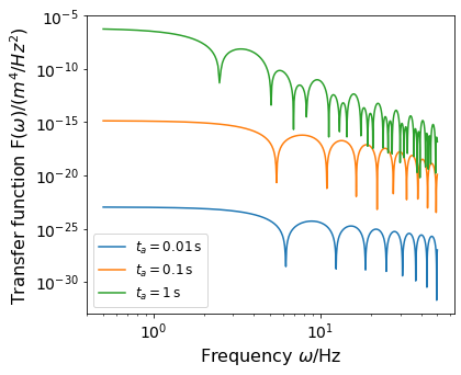
(a) (a)

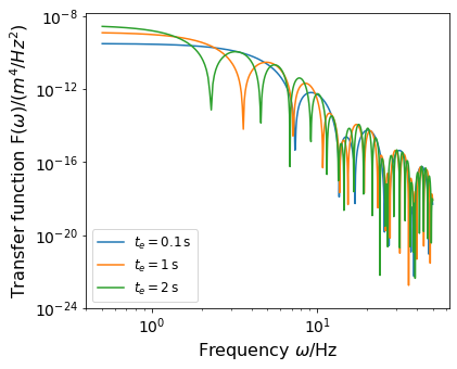
(b) (b)

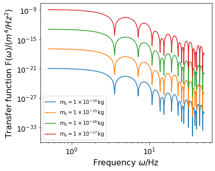
(c) (c)

Figure 2: We have shown the transfer function for the interferometer shown in Fig. 1 for different experimental parameters. The fixed parameters is $\nabla B=10^{4}$ T/m in all the figures. The other parameters are set to be: $m_{0}=10^{-17}$ kg (corresponds to $a_{m}=1.8\times 10^{-2}\rm\,m/s^{2}$) and $t_{e}=1$ s in the sub-figure (a), $m_{0}=10^{-17}$ kg and $t_{a}=0.5$ s in the sub-figure (b), and $t_{a}=0.5$ s and $t_{e}=1$ s in the sub-figure (c). As we have shown in all the figures, the transfer function $F(\omega)$ approaches a constant value in the low-frequency range, and decreases as a polynomial of $\omega$ in the high-frequency rregime. By comparing the sub-figures (a) with (b), we can find that the transfer function $F(\omega)$ is more sensitive to the value of the splitting time $t_{a}$, than the free-falling time $t_{e}$, especially in the low-frequency range. As we can see from the sub-figure (c), the transfer function $F(\omega)\propto m_{0}^{-4}$.

We consider the specific configuration shown in Fig. 1  Marshman:2018upe . The interferometer is set to freely fall, and the creation and recombination stages control the superposition along the $x$-axis. For simplicity, the acceleration during the splitting and recombining parts is assumed to be constant, which can be achieved in a Stern-Gerlach apparatus with constant magnetic field gradient. The absolute value of the acceleration is given by, see PhysRevLett.119.240401 ; Toros:2020dbf .

$$a_{m}=\frac{g\mu_{B}}{m_{0}}|\nabla B|,$$ (8)

where $g=2$ is the Lande g-factor, $\mu_{B}=9\times 10^{-24}$ J/T is the Bohr magneton, $m_{0}$ is the mass of the interferometer and $\nabla B=10^{4}$ T/m Nat.Commun.4.2424 ; Marshman:2021wyk ; Henkel:2021wmj is the gradient of the magnetic field. The direction of the acceleration $a_{m}$ depends on the gradient of the magnetic field, and the value of the spin in each arm. The magnetic field gradient makes the system on the right path accelerate during $[0,t_{a}]$ and $[2t_{a}+t_{e},3t_{a}+t_{e}]$, decelerate during $[t_{a},2t_{a}]$ and $[3t_{a}+t_{e},4t_{a}+t_{e}]$, while in the intermediate interval $[2t_{a},2t_{a}+t_{e}]$ it is vanishingly small, while the part of the system on the left path is in free-fall. The transfer function for such an interferometer is given by :

$$F(\omega)= 16\frac{a_{m}^{4}}{\omega^{10}}\bigg{(}-t_{a}^{2}\omega^{2}\sin\left(\omega(t_{a}+t_{e}/2)\right)$$

$$+\left(t_{a}^{2}\omega^{2}+3\right)\sin\left(t_{e}\omega/2\right)-3\sin\left(\omega(2t_{a}+t_{e}/2)\right)$$

$$+6t_{a}\omega\cos\left(\omega(t_{a}+t_{e}/2)\right)\bigg{)}^{2}.$$ (9)

The transfer function $F(\omega)$ is plotted in Fig. 2 with different values for the splitting time $t_{a}$, the free-falling time $t_{e}$, and the interferometer mass $m_{0}$.

As we have shown in sub-figures (a) and (b) of Fig. 2, the splitting time, $t_{a}$, and the free-falling time, $t_{e}$, significantly affect on the behaviour of the transfer function $F(\omega)$. The splitting time has a greater impact on the absolute value of $F(\omega)$, while the free-falling time has a greater impact on the oscillatory behaviour of $F(\omega)$.

At low frequency, $\omega\ll 2\pi/(4t_{a}+t_{e})$, one can find that $F(\omega)$ reaches the constant value  $\Delta x^{4}(23t_{a}+15t_{e})^{2}/225$, which is much more sensitive to the value of $t_{a}$ than to the value of $t_{e}$. Setting $t_{e}=0$, we find a simple formula for the transfer function in the low frequency regime:

$$\bar{F}\equiv\lim_{\omega\rightarrow 0}F(\omega)=\frac{529}{225}\Delta x^{4}t_{a}^{2}.$$ (10)

In the high-frequency region, $\omega\gg 2\pi/(4t_{a}+t_{e})$, the transfer function $F(\omega)$ decreases rapidly as $\propto\omega^{-6}$.

As we have shown in Fig. 2 (c), the influence of the mass on the transfer function is a simple rescaling as $F(\omega)\propto m_{0}^{-4}$ according to Eqs. (8) and (9). However, an interesting result is that for the configuration discussed in Appendix B, the corresponding transfer function $F(\omega)\propto m_{0}^{-2}$, which leads to $\Gamma_{\rm noise}\propto m_{0}^{2}F(\omega)$, a mass-independent phase fluctuation.

III GGN in matter-wave interferometers

In this section, we will analyse the phase fluctuation density due to the GGN. In the Fermi normal coordinate system, constructed near the worldline of the laboratory Poisson2011 , the Lagrangian in a non-relativistic limit is given by Toros:2020dbf

$$L_{\rm free-falling}=\frac{1}{2}m_{0}v^{2}-m_{0}a_{0}x-\frac{1}{2}m_{0}\underbrace{R_{0101}c^{2}}_{\equiv\omega_{gg}^{2}(t)}x^{2},$$ (11)

where the superposition direction is defined along the $x$-axis as shown in Fig. 1. The first term on the right-hand side of Eq. (11) corresponds to a free-falling particle in a flat spacetime, and the other terms $m_{0}a_{0}x$ and $\frac{1}{2}m_{0}R_{0101}c^{2}x^{2}$ can be regarded as the acceleration noise and the GGN caused by the fluctuations in the metric, respectively Toros:2020dbf .

For a free-falling experiment, the acceleration term $a_{0}$ will vanish according to the properties of the Fermi normal coordinates (in line with Einstein’s equivalence principle), so this noise will be neglected in this paper. Therefore, we will solely focus on the noise $\omega_{gg}^{2}(t)$ in Eq. (11), which corresponds to the noise $\omega_{\rm noise}^{2}$ in Sec. II. As discussed, we characterize such a stochastic quantity by the noise PSD (see Eq. (4)). In particular, we introduce the GGN PSD, $S_{gg}(\omega)$, by the inverse-Fourier transformation, that is

$$S_{gg}(\omega)= \int\mathbb{E}[\omega_{gg}^{2}(t)\omega_{gg}^{2}(t+\tau)]\mathrm{e}^{i\omega\tau}d\tau$$

$$\int\mathbb{E}[R_{0101}(t)R_{0101}(t+\tau)]c^{4}\mathrm{e}^{i\omega\tau}d\tau,$$ (12)

which has units of [$\rm Hz^{4}/Hz$] . There are many sources of GGN as noted inPhysRevD.58.122002 ; PhysRevD.60.082001 ; Beccaria:1998ap ; Harms2019 , but in this paper we will focus on one particular source of GGN due to the smooth motion of external objects. In the next section we first adapt the two-dimensional classical analysis from  PhysRevD.30.732 to matter-wave interferometry in three-spatial dimensions.

IV Three dimensional GGN

Figure 3: Three-dimensional GGN caused by the smooth motion of an external object. The external object is located at a point $(x,\ y,\ z)$ at time $t$, and moves with a constant velocity $\vec{v}=(v_{x},v_{y},v_{z})$, while the interferometer of mass $m_{0}$ is located at the origin, with the superposition along the $x$-axis. The impact parameter is denoted here as $b$, and the projection angles are defined as $\cos\alpha=x_{0}/b$ and $\cos\beta=v_{x}/v$, where $x_{0}$ is the x-coordinate at $t=0$ and $v_{x}$ is the x-component of the constant velocity $\vec{v}$.

To quantify the achievable sensitivity for measuring the GGN in three spatial dimensions, we first compute the corresponding PSD $S_{gg}(\omega)$. Consider the model shown in Fig. 3, and suppose that the external object whose coordinate is denoted by $\vec{r}=(x,\ y,\ z)$ moves with a uniform velocity $\vec{v}=(v_{x},\ v_{y},\ v_{z})$, and with an impact parameter $b$. Then the local acceleration of the interferometer caused by the external mass at a given time, $t$, will be given by:

$$\begin{split}\vec{a}(t)&=\frac{GM}{r^{2}(t)}\frac{\vec{r}(t)}{r(t)}\\ &=\frac{GM}{r^{3}(t)}x(t)\vec{e}_{x}+\frac{GM}{r^{3}(t)}y(t)\vec{e}_{y}+\frac{GM}{r^{3}(t)}z(t)\vec{e}_{z},\end{split}$$ (13)

where $\vec{e}_{j}$ ($j=x,y,z$) are the unit basis vectors. Since the external mass is assumed to be moving with a uniform velocity, one can write down $r^{2}(t)=b^{2}+v^{2}t^{2}$ and $x(t)=x_{0}+v_{x}t$ if $t=0$ is defined as the time when the external object is at the closest point. Further, if we introduce the projection angles

$$\cos\alpha=x_{0}/b,~{}~{}\cos\beta=v_{x}/v,$$ (14)

then the $x$-direction component of the acceleration $\vec{a}$ can be written as

$$\begin{split}a_{x}(t)&=\frac{GM}{b^{2}}\frac{x_{0}/b+v_{x}t/b}{(1+v^{2}t^{2}/b^{2})^{3/2}}\\ &=\frac{GM}{b^{2}}\frac{\cos\alpha+(vt/b)\cos\beta}{(1+v^{2}t^{2}/b^{2})^{3/2}}.\end{split}$$ (15)

Then in the frequency space, the Fourier transform of $a_{x}(t)$ is given by 

$$\begin{split}a_{x}(\omega)=&\frac{GM}{b^{2}}\left(\frac{\omega b}{v}\right)\left[\frac{x_{0}}{v}K_{1}\left(\frac{\omega b}{v}\right)+i\frac{b}{v}\frac{v_{x}}{v}K_{0}\left(\frac{\omega b}{v}\right)\right]\\ =&\frac{a_{\text{loc}}}{\omega}u_{\omega}^{2}\left[\cos\alpha K_{1}\left(u_{\omega}\right)+i\cos\beta K_{0}\left(u_{\omega}\right)\right],\end{split}$$ (16)

where $K_{0}(\;\cdot\;)$ and $K_{1}(\;\cdot\;)$ are the modified Bessel functions. In the second line of Eq. (16) we have introduced the local acceleration, $a_{\rm loc}$, and the frequency-dependent dimensionless ratio, $u_{\omega}$, defined as

$$a_{\rm loc}\equiv GM/b^{2},\;\;\;u_{\omega}\equiv\omega b/v,$$ (17)

which, as we will see, control the behaviour of the GGN.

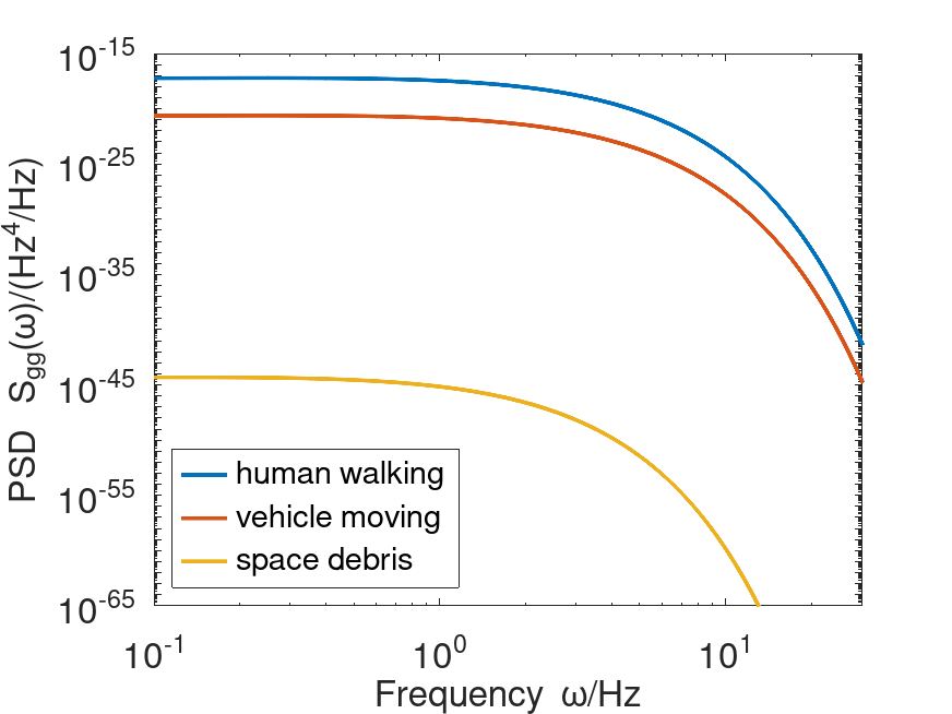
Figure 4: We have shown the PSD of the GGN for several sources, including human walking, vehicles moving, and space debris according to Eq. (20). The masses are set as $50$ kg, $10^{3}$ kg and $10^{3}$ kg in respect, the speeds are $1$ m/s, $10$ m/s and $5\times 10^{4}$ m/s respectively, and the impact parameter is set as $1$ m, $10$ m and $10^{5}$ m in respect. As shown in the gravitational-wave literature Harms2019 ; Acernese_2014 ; Bader_2022 , the GGN usually has a dominant contribution in the low-frequency range. The PSD for the GGN is usually smaller than $10^{-20}\,\rm Hz^{4}/Hz$ Acernese_2014 ; Bader_2022 , while it can reach $10^{-15}\,\rm Hz^{4}/Hz$ level for the human walking, and this is the reason why an ultra-sensitive experiment requires an exclusion zone for human activities PhysRevD.30.732 ; PhysRevD.60.082001 ; Toros:2020dbf . In this work, we, however, propose to detect such a tiny GGN as a signal by designing a suitable interferometer, i.e., by optimising the transfer function in Eq. (9). As we discuss in the text, by tuning the interferometric times, we can obtain a transfer function which can induce a detectable phase fluctuation, $\Gamma_{gg}$, in the specific frequency range.

The PSD of the acceleration noise on $a_{x}(\omega)$ can be computed as  

$$S_{aa}(\omega)=\frac{|a_{x}(\omega)|^{2}}{T},$$ (18)

where $T$ is the scattering time between the external mass and the interferometer (in this context, playing the role of the signal and sensor, respectively). A rough estimation of $T\sim b/v$, because the moving object is at a distance, ($r(t)=\sqrt{v^{2}t^{2}+b^{2}}$), that the interaction becomes negligible after $T\geq b/v$. An exact estimation of $T\sim b/v$ was also made in Ref. PhysRevD.30.732 . We have particularly chosen the same estimation to match those results for two and three dimensions, discussed in the Appendix A. By combining Eqs. (16) and (18), we can obtain the PSD for the acceleration noise,

$$S_{aa}(\omega)=\frac{a_{\rm loc}^{2}}{\omega}u_{\omega}^{3}\big{[}\cos^{2}\alpha K_{1}^{2}\left(u_{\omega}\right)+\cos^{2}\beta K_{0}^{2}\left(u_{\omega}\right)\big{]}.$$ (19)

Since the local acceleration $a_{\rm loc}$ is caused by the fluctuation of the local spacetime curvature, one may have the relation $a_{\rm loc}\sim R_{0101}c^{2}b$ , then the PSD for the local acceleration satisfies $S_{aa}(\omega)\sim S_{gg}(\omega)b^{2}$. Finally, the PSD of the GGN is given by

$$S_{gg}(\omega)=\frac{a_{\rm loc}^{2}}{\omega b^{2}}u_{\omega}^{3}\left[\cos^{2}\alpha K_{1}^{2}\left(u_{\omega}\right)+\cos^{2}\beta K_{0}^{2}\left(u_{\omega}\right)\right].$$ (20)

For example, the PSD of several sources such as human walking, vehicles moving, and space debris moving with a constant velocity is shown in Fig. 4. In gravitational-wave interferometers, $S_{gg}(\omega)$ is regarded as a source of noise, and is mitigated from $10^{-15}\,\rm Hz^{4}/Hz$ down to about $10^{-20}\,\rm Hz^{4}/Hz$ for human walking by setting a suitable exclusion zonesAcernese_2014 ; Bader_2022 ; PhysRevD.30.732 ; PhysRevD.60.082001 ; Toros:2020dbf .

We want to devise an interferometer that is capable of detecting weak GGN as signals in the low-frequency range by optimising the interferometric parameters. From Eqs. (5) and (20), we find that the the corresponding phase fluctuation is given by

$$\Gamma_{gg}= \left(\frac{2m_{0}a_{\rm loc}}{\hbar b}\right)^{2}\ \int\frac{u_{\omega}^{3}F(\omega)}{\omega}$$

$$\left[\cos^{2}\alpha K_{1}^{2}\left(u_{\omega}\right)+\cos^{2}\beta K_{0}^{2}\left(u_{\omega}\right)\right]d\omega.$$ (21)

Note that the PSD for the GGN $S_{gg}(\omega)$ approximately converges to zero in the low-frequency limit $\omega\to 0^{+}$, while the transfer function $F(\omega)$ converges to a non-zero constant, so the lower bound $\omega_{\rm min}=2\pi/t_{\rm exp}$ of the integration is not so relavant for the total phase fluctuation, $\Gamma_{gg}$. However, it still matters for some other sources of noise which diverges in the low frequency region, see  Toros:2020dbf .

In experiments, the minimum measurable value of $\Gamma_{gg}$ will be determined by the the overall phase sensitivity. In the following we will assume $\Gamma_{gg}=0.01$ as a threshold value below which we can no longer reliably measure the phase fluctuations. Given such a threshold value for $\Gamma_{gg}$ we can then ask what should be the characteristic of the interferometer, such that it can discern a particular GGN as a signal. The interferometer mass, $m_{0}$, and the the superposition size, $\Delta x$, control the overall amplitude of the signal, while the beam-splitting time, $t_{a}$, and the free-fall time, $t_{e}$, control the sensitivity in a particular frequency range.

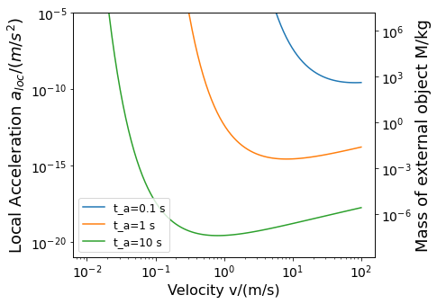
(a) (a)

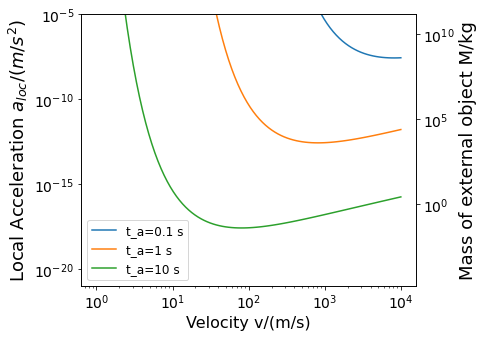
(b) (b)

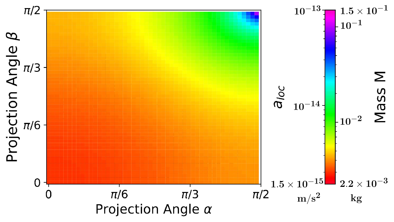
(c) (c)

Figure 5: (a) The left-most panel shows the plot of the minimum detectable local acceleration, $a_{\text{loc}}=GM/b^{2}$ (left vertical-axis), or equivalently, the minimum detectable mass of the GGN source (right vertical-axis). The GGN source has an impact parameter $b=10$ m and velocity v (horizontal-axis). The GGN sensitivity increases by increasing the beam-splitting time $t_{a}$ (the free-falling time $t_{e}=0$ s for simplicity such that the total interferometric time is $4t_{a}$. The beam-splitting acceleration $a_{m}$ is set as $1.8\times 10^{-2}\rm\,m/s^{2}$ (the corresponding magnetic field gradient we have used here is $\nabla B=10^{4}$ T/m), and the mass of the interferometer is $m_{0}=10^{-17}$ kg. (b) The middle panel shows similar to (a) but with the impact parameter set to $b=1000$ m, requiring longer beam-splitting times $t_{a}$ to achieve the same sensitivity for the minimum detectable mass (corresponding to a better sensitivity of the minimum detectable local acceleration). (c) The right most panel shows the colour map for the minimum detectable local acceleration as a function of the projection angles $\alpha$ (horizontal-axis) and $\beta$ (vertical-axis) quantifying the relative orientation of the interferometer and the motion of the external object (see Fig. 3). The impact factor has been set to $b=10$ m and the velocity to $v=10$ m/s. The optimal sensitivity is achieved when the motion of the external object is aligned with the axis of the interferometer ($\alpha=0$ and $\beta=0$).

From Eq. (21) we can find the local gravitational acceleration

$$a_{\rm loc}(M)=\frac{\hbar b\sqrt{\Gamma_{gg}}}{2m_{0}}\bigg{(} \int\frac{u_{\omega}^{3}F(\omega)}{\omega}\big{(}\cos^{2}\alpha K_{1}^{2}\left(u_{\omega}\right)$$

$$+\cos^{2}\beta K_{0}^{2}\left(u_{\omega}\right)\big{)}d\omega\bigg{)}^{-1/2},$$ (22)

where the right-hand side fixes all the parameters, except the mass $M$ of the external object. Eq. (IV) thus provides a simple expression to estimate the minimum acceleration that one can sense given the threshold phase sensitivity $\Gamma_{gg}$. Since the impact parameter, $b$ is also fixed on the right-hand side of Eq. (IV) we find from Eq. (17) that the minimum detectable mass $M$ of the external object with impact factor $b$ (moving with velocity $v$, and with its direction parametrised by the angles $\alpha$ and $\beta$), is given by $M=a_{\rm loc}b^{2}/G$.

V Sensing GGN sources in an earth-based laboratories and space-debris in the vicinity of satellites

We now apply the model developed in the previous sections to sense GGN from two different types of sources. For simplicity we will set the free-fall time to $t_{e}=0$ and vary only the beam-splitting time $t_{a}$. We will focus on sensing GGN in the vicinity of Earth-based laboratories and sensing space-debris in the vicinity of satellites (Sec. V). The goal of this section is to check the feasibility of tracking the motion of the objects, ideally in real-time, and hence we consider the total experimental time to be the smallest possible, i.e., $t_{\text{exp}}=4t_{a}$. To make a statistically significant number of experimental runs we would thus need to consider an array of interferometers operating simultaneously.

Now we quantify the sensitivity to GGN signals caused by the motion of small objects in the proximity of experiments. As we will see, unknown light objects, even if moving at slow speeds, can be a significant source of GGN for state-of-the-art experiments, which become sensitive to tiny local accelerations.

We first focus on GGN sources that could be present inside earth-based laboratories. In particular, we will consider external objects in the velocity range $(10^{-2}-10^{2})\,{\rm m/s}$, and with masses in the range from $(10^{-5}-10^{3})$ kg. We will further assume that the external object, acting as the GGN source, has an impact factor $b=10$ m.

As discussed in Sec. IV we will set the GGN phase to the value $\Gamma_{gg}\geq 0.01$ . If one fixes also the beam-splitting time $t_{a}$ one can then evaluate the local acceleration $a_{\rm loc}$. Using Eq. (17) one can then readily determine also the minimum detectable mass $M$ of the GGN source.

As shown in Fig. 5 (a), when $v\to 0$ or $v\to\infty$, the local acceleration $a_{\rm loc}$ tends to infinity and the minimum detectable mass $M$ becomes extremely large. Indeed, when the external object moves too slowly or too fast, its GGN signal decreases as the frequency range of the interferometer $\sim t_{a}^{-1}$ is no longer compatible with the characteristic frequency of the GGN source given by $v/b$. The interferometer performs optimally as a GGN sensor when $t_{a}$ is comparable to $b/v$.

A similar analysis as discussed above can be also adapted for sensing space debris in the vicinity of satellites article ; Cowardin2017CharacterizationOO . For illustration, we will consider the debris at impact factor $b=1000$ m and with velocity in the range $(10^{0}-10^{4})\,{\rm m/s}$. We consider the same beam-splitting times as in the previous section, although the beam-splitting time could be significantly extended in space aveline2020observation ; gasbarri2021testing . In Fig. 5 (b) we show the measurable local acceleration, or equivalently, the minimum detectable mass of the GGN source.

In Fig. 5 (c) we also show the minimum detectable mass as a function of the projection, $\cos\alpha$ and $\cos\beta$, defined in Eq. (14) evaluated for a fixed beam-splitting time $t_{a}$, fixed velocity $v=10$ m/s, and fixed impact factor $b=10$ m. The optimal sensitivity is achieved for $\cos\alpha=\cos\beta=1$ corresponding the external object moving along the $x$-axis.

VI Summary

In this paper, we first made a brief review of frequency-space analysis for matter-wave interferometry. We pointed out that the spectral density of the phase fluctuation caused by a noise can be always factorized into the noise part (described by the corresponding PSD) and the trajectory part (described by the so-called transfer function defined by Eq. (II)). Although we have primarily focused on a SG scheme with nanoparticles, a similar analysis could be readily adapted to other types of matter-wave interferometers, such as those based on ultra-cold atom Bose-Einstein Condensate (BEC)Peters1999 ; PhysRevLett.120.183604 ; PhysRevLett.125.191101 ; gravitational_AB_effect ; science.abm6854 .

We have developed a 3D model for the GGN signal of a moving external object, and obtained the corresponding PSD in Eq. (20), generalizing the two dimensional model in PhysRevD.30.732 . Based on the PSD of gravity gradient signal, we then derived the expression Eq. (IV) and Eq. (26), which quantifies the local gravitational acceleration, or equivalently, the minimum detectable mass of the GGN source.

Finally, we applied the developed model to investigate two distinct GGN sources, namely, slow moving objects in Earth-based laboratories and space debris near satellites, and studied how the GGN signal varies with the velocity, distance, and orientation.

Of course, there are numerous challenges to be met before we can realize experimentally such a quantum sensor. Creating large spatial superpositions and achieving the required coherence time with large masses is a formidable challenge. Nonetheless, we foresee that a nanoparticle matter-wave interferometer can have many novel technological applications, complementing the fundamental tests of Newton’s law or detecting the quantum gravity induced entanglement.

Appendix A Three Dimensional GGN and Reduction to two Dimensions

The model established in Sec. IV is a generalisation of a well-known model discussed in Ref. PhysRevD.30.732 . In this appendix, we will discuss the special cases of the 3 dimensional model, and show how it reduces to the results of 1-dimensional model of Ref. PhysRevD.30.732 .

A.1 Three dimensional model

When $\omega b/v\gg 1$, we can make some approximations which are useful to investigate the slowly moving external objects (see Sec. V). In this latter regime, the modified Bessel functions can be approximated as

$$K_{0}\left(u_{\omega}\right)\approx K_{1}\left(u_{\omega}\right)\approx\sqrt{\frac{\pi}{2}}\frac{e^{-u_{\omega}}}{\sqrt{u_{\omega}}}.$$ (23)

Then the PSD for the GGN in Eq. (20) can be reduced to:

$$S_{gg}(\omega)=\frac{a_{\text{loc}}^{2}}{\omega b^{2}}u_{\omega}^{2}(\cos^{2}\alpha+\cos^{2}\beta)e^{-2u_{\omega}}.$$ (24)

Note that when, $\alpha=0$, and, $\beta=\pi/2$, the PSD can be further reduced to

$$S_{gg}(\omega)=\frac{a_{\text{loc}}^{2}}{\omega b^{2}}u_{\omega}^{2}e^{-2u_{\omega}},$$ (25)

which is the same result in Ref. PhysRevD.30.732 . Based on the reduced PSD in Eq. (24), the local acceleration, Eq. (IV), can be simplified to

$$a_{\rm loc}=\frac{\hbar v}{2m_{0}}\sqrt{\frac{\Gamma_{gg}}{(\cos^{2}\alpha+\cos^{2}\beta)\int\omega F(\omega)e^{-2u_{\omega}}d\omega}}.$$ (26)

Physically, the condition, $\omega b/v\geq 1$, gives, $b/v\geq 1/\omega_{\rm min}\sim t_{\rm exp}$, which constrains the interaction time, $T\sim b/v$, to be longer than the interferometric times, $t_{a},~{}t_{e}$. For example, a walking person who is moving with the speed $\sim 1$ m/s, at a distance, $\sim 1$ m, so the corresponding ratio $b/v\sim 1$ s satisfies the condition $b/v\geq t_{\rm e},t_{\rm a}\sim 1$ s.

However, the approximation in Eq. (26) gives reasonable values as long as we are in the regime $\tilde{\omega}_{j}b/v\gg 1$, where $\tilde{\omega}_{j}=2\pi/t_{j}$ ($j=a,e$) denotes the characteristic frequencies of the interferometer. The latter regime has the following hierarchy of times:

$$t_{a},t_{e}\ll b/v\ll t_{\text{exp}},$$ (27)

where we recall that $t_{\text{exp}}$ is the total experimental time, $b/v$ can be interpreted as the interaction time, and $t_{a},t_{e}$ are the beam-splitting time and free-evolution time of a single interferometric loop, respectively. In such a regime we can make the approximation $F(\omega)\approx\bar{F}$, where $\bar{F}$ is defined in Eq. (10). The integrations in Eq. (IV) then reduce to

$$\int_{0}^{\infty}u_{\omega}^{2}K_{0}^{2}\left(u_{\omega}\right)du_{\omega} =\frac{\pi^{2}}{32}\approx 0.31,$$ (28)

$$\int_{0}^{\infty}u_{\omega}^{2}K_{1}^{2}\left(u_{\omega}\right)du_{\omega} =\frac{3\pi^{2}}{32}\approx 0.93,$$ (29)

where we have changed the integration variable to $u_{\omega}=b\omega/v$ defined in Eq. (17). On the other hand, using the approximation in Eq. (23), the relevant integration in Eq. (IV) evaluates to:

$$\int_{0}^{\infty}u_{\omega}\left(\sqrt{\frac{\pi}{2}}\frac{e^{-u_{\omega}}}{\sqrt{u_{\omega}}}\right)^{2}du_{\omega}=\frac{\pi}{8}\approx 0.40.$$ (30)

which is of the same order of magnitude as the results obtained in Eqs. (28) and (29). Since in this work we are primarily interested in the order of magnitude estimates, we will thus use the approximation in Eq. (26) also for the regime given in Eq. (27).

A.2 GGN in two dimensions

Figure 6: The two dimensional model for the GGN caused by a smooth motion. The external object is originally located at point $(b,\ \theta_{0})$, and moves with a constant speed $v$.

Now we will show how the three dimensional model developed in Sec. IV reduces to a two-dimensional model when the external object and the quantum sensor are confined to a plane (see Fig. 6). Comparing to the three dimensional model from the main text, we only need one polar angle $\theta$ to describe the motion of the external object moving at impact factor $b$. As we will see below, if we further set the angle to $\theta_{0}=0$, then the two dimensional model reduces to the original model proposed in PhysRevD.30.732 . The acceleration caused by the Newtonian force in the x-direction is given by:

$$a_{x}(t)=\frac{GM}{b^{2}}\frac{1}{(1+(vt/b)^{2})^{3/2}}(\cos\theta_{0}+(vt/b)\sin\theta_{0}),$$ (31)

so in the frequency space, the local acceleration is

$$a_{x}(\omega)=\frac{GM}{b^{2}\omega}u_{\omega}^{2}\left(\cos\theta_{0}K_{1}\left(u_{\omega}\right)+i\sin\theta_{0}K_{0}\left(u_{\omega}\right)\right),$$ (32)

where $K_{\alpha}(\;\cdot\;)$ is the modified Bessel function, and we have introduced $u_{\omega}=b\omega/v$ (see Eq. (17) in the main text). Comparing to the three dimensional result in Eq. (16), the projection angle $\alpha$ and $\beta$ becomes $\theta_{0}$ and $\pi/2-\theta_{0}$, respectively.

According to $S_{aa}(\omega)=|a_{x}(\omega)|^{2}/T$, $T=b/v$, and $S_{gg}(\omega)=S_{aa}(\omega)/b^{2}$, the PSD for the GGN in the two dimensional case is given by:

$$S_{gg}(\omega)=\frac{a_{\text{loc}}^{2}u_{\omega}^{3}}{\omega b^{2}}\left[\cos^{2}\theta_{0}K_{1}^{2}\left(u_{\omega}\right)+\sin^{2}\theta_{0}K_{0}^{2}\left(u_{\omega}\right)\right],$$ (33)

where we have introduced, $a_{\text{loc}}=GM/b^{2}$ (see Eq. (17) in the main text). The corresponding phase fluctuation is given by:

$$\Gamma_{gg}= \left(\frac{2m_{0}a_{\rm loc}}{\hbar b}\right)^{2}\ \int\frac{u_{\omega}^{3}F(\omega)}{\omega}$$

$$\left[\cos^{2}\theta_{0}K_{1}^{2}\left(u_{\omega}\right)+\sin^{2}\theta_{0}K_{0}^{2}\left(u_{\omega}\right)\right]d\omega.$$ (34)

From Eq. (34) we then readily find the local acceleration:

$$a_{\rm loc}(M)=\frac{\hbar b\sqrt{\Gamma_{gg}}}{2m_{0}}\bigg{(} \int\frac{u_{\omega}^{3}F(\omega)}{\omega}\big{(}\cos^{2}\theta_{0}K_{1}^{2}\left(u_{\omega}\right)$$

$$+\sin^{2}\theta_{0}K_{0}^{2}\left(u_{\omega}\right)\big{)}d\omega\bigg{)}^{-1/2}.$$ (35)

If we now set $\theta_{0}=0$, we recover the result presented in PhysRevD.30.732 . In the regime, $u_{\omega}\gg 1$, the modified Bessel’s function can be approximated as $K_{0}(u_{\omega})\sim K_{1}(u_{\omega})\sim e^{-u_{\omega}}/u_{\omega}^{1/2}$ (see Eq. (23)). In this regime, the PSD for the GGN in Eq. (33) reduces to

$$S_{gg}(\omega)=\frac{a_{\text{loc}}^{2}}{b^{2}\omega}u_{\omega}^{2}e^{-2\omega b/v}.$$ (36)

The GGN formula Eq. (36) remains a decent approximation even when $u_{\omega}\sim 1$ which is the regime considered in  PhysRevD.30.732 where they have omitted the dimensionless prefactor $u_{\omega}^{2}$. Besides, as is seen in (36), the choice of $T$ should be $b/v$ to match the result in PhysRevD.30.732 , otherwise there will be an additional factor. Finally, using Eq. (36) we find that the local acceleration simplifies to the simple expression:

$$a_{\rm loc}=\frac{\hbar v}{2m_{0}}\sqrt{\frac{\Gamma_{gg}}{\int\omega F(\omega)e^{-2u_{\omega}}d\omega}},$$ (37)

which matches Eq. (26) for $\alpha=0$ and $\beta=\pi/2$.

Appendix B GGN with two symmetric interferometers

Figure 7: Illustration of the paths of the dual interferometer. A single symmetric interferometer is by itself not susceptible to sense GGN, because one can always choose the origin of the coordinate system, corresponding to the origin of the harmonic GGN metric perturbation, such that the paths are located symmetrically on each side (for example, the paths of the right interferometer are symmetric with respect to $x=d/2$ and the phases on each arm would become proportional to $\propto(\pm\Delta x/2)^{2}$ – one only generates an undetectable global phase on an individual interferometer). However, if one is considering joint observables of multiple interferometers placed along the $x$-axis, one can no longer make the phases on an individual interferometer $\propto x^{2}$ equal, leading to a nonzero GGN signal. Indeed, in the picture the phases on the two arms of the left (right) interferometer are given by $\propto(-d/2\pm\Delta x/2)^{2}$ ($\propto(d/2\pm\Delta x/2)^{2}$). More generally, two or more adjacent symmetric interferometers can become sensitive to GGN when the two arms of an individual individual interferometer are placed asymmetrically with respect to the origin of the local GGN metric pertubation Toros:2020dbf . $d$ is the distance between the two interferometers, and $\Delta x$ is the superposition size, assumed equal for both interferometers.

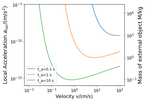
(a) (a)

(b) (b)

(c) (c)

Figure 8: Same as Fig. 5 but for the dual interferometer in Fig. 7 with the transfer function given in Eq. (38). The mass of an individual interferometer is $m_{0}=10^{-17}$ kg, and we have set the distance between the two interferometers to $d=100\,\mu$m, the splitting time $t_{a}=1$ s, the free-falling time $t_{e}=$0 s and the beam-splitting acceleration $a_{m}=1.8\times 10^{-2}\rm\,m/s^{2}$ corresponding to the magnetic field gradient $\nabla B=10^{4}$ T/m. (a) Plot of minimum detectable local acceleration, or equivalently, of the minimum detectable mass of the GGN source. The impact factor is set to $b=10$ m. (b) Same as (a) but with the impact parameter set to $b=1000$ m. (c) Colour map for the minimum detectable local acceleration as a function of the projection angles $\alpha$ and $\beta$. The impact factor of the external object has been set to $b=10$ m and the velocity to $v=10$ m/s.

For completeness we discuss the dual QGEM interferometer depicted in Fig. 7. Each individual interferometer (the left one or the right one) has the paths located asymmetrically with respect to the origin – as such, the two paths of an individual interferometer acquire a nonzero phase difference from the harmonic trap generated by a GGN signal centered at the origin. In case, one is looking at joint properties of the two interferometers, such as an entanglement witness, the dual interferometer becomes sensitive to GGN Toros:2020dbf .

The transfer function for symmetric interferometer is given by Toros:2020dbf :

$$F(\omega)=64d^{2}a_{m}^{2}\frac{\sin^{4}(\frac{\omega t_{a}}{2})\sin^{2}(\frac{1}{2}\omega(2t_{a}+t_{e}))}{\omega^{6}}.$$ (38)

where $d$ denotes the distance between the centers of two interferometers (the rest of the parameters have the same meaning to the ones defined in the main text).

An interesting observation is that the transfer function for this configuration is proportional to $m_{0}^{-2}$ rather than $m_{0}^{-4}$ in Eq. (9). As a consequence the corresponding phase fluctuation density $\Gamma_{\rm noise}$ will be independent of $m_{0}$, according to Eq. (5). Thus, the mass of the superposition can be chosen arbitrarily for this configuration, which is an advantage. We have discussed the minimum local acceleration, or equivalently, the minimum detectable mass, from sensing GGN in Fig. 8. We note that the dual QGEM interferometer is less sensitive to sense the GGN in comparison to the asymmetric MIMAC interferometer.

References

- (1) Kai Bongs and Klaus Sengstock. Physics with coherent matter waves. Reports on Progress in Physics, 67(6):907–963, may 2004.
- (2) Chris Overstreet, Peter Asenbaum, Tim Kovachy, Remy Notermans, Jason M. Hogan, and Mark A. Kasevich. Effective inertial frame in an atom interferometric test of the equivalence principle. Phys. Rev. Lett., 120:183604, May 2018.
- (3) Peter Asenbaum, Chris Overstreet, Minjeong Kim, Joseph Curti, and Mark A. Kasevich. Atom-interferometric test of the equivalence principle at the level. Phys. Rev. Lett., 125:191101, Nov 2020.
- (4) Sougato Bose, Anupam Mazumdar, Martine Schut, and Marko Toroš. Entanglement Witness for the Weak Equivalence Principle. 3 2022.
- (5) Achim Peters, Keng Yeow Chung, and Steven Chu. Measurement of gravitational acceleration by dropping atoms. Nature, 400(6747):849–852, Aug 1999.
- (6) Ryan J. Marshman, Anupam Mazumdar, Gavin W. Morley, Peter F. Barker, Steven Hoekstra, and Sougato Bose. Mesoscopic Interference for Metric and Curvature (MIMAC) Gravitational Wave Detection. New J. Phys., 22(8):083012, 2020.
- (7) Raymond Y. Chiao and Achilles D. Speliotopoulos. Towards MIGO, the Matter wave Interferometric Gravitational wave Observatory, and the intersection of quantum mechanics with general relativity. J. Mod. Opt., 51:861, 2004.
- (8) Albert Roura, Dieter R. Brill, B. L. Hu, and Charles W. Misner. Gravitational wave detectors based on matter wave interferometers (MIGO) are no better than laser interferometers (LIGO). Phys. Rev. D, 73:084018, 2006.
- (9) Stefano Foffa, Alice Gasparini, Michele Papucci, and Riccardo Sturani. Sensitivity of a small matter-wave interferometer to gravitational waves. Phys. Rev. D, 73:022001, 2006.
- (10) Savas Dimopoulos, Peter W. Graham, Jason M. Hogan, Mark A. Kasevich, and Surjeet Rajendran. An Atomic Gravitational Wave Interferometric Sensor (AGIS). Phys. Rev. D, 78:122002, 2008.
- (11) Savas Dimopoulos, Peter W. Graham, Jason M. Hogan, Mark A. Kasevich, and Surjeet Rajendran. Gravitational Wave Detection with Atom Interferometry. Phys. Lett. B, 678:37–40, 2009.
- (12) Guglielmo M. Tino et al. SAGE: A Proposal for a Space Atomic Gravity Explorer. Eur. Phys. J. D, 73(11):228, 2019.
- (13) Peter Asenbaum, Chris Overstreet, Minjeong Kim, Joseph Curti, and Mark A. Kasevich. Atom-Interferometric Test of the Equivalence Principle at the Level. Phys. Rev. Lett., 125(19):191101, 2020.
- (14) Peter W. Graham, Jason M. Hogan, Mark A. Kasevich, and Surjeet Rajendran. A New Method for Gravitational Wave Detection with Atomic Sensors. Phys. Rev. Lett., 110:171102, 2013.
- (15) R. Colella, A. W. Overhauser, and S. A. Werner. Observation of gravitationally induced quantum interference. Phys. Rev. Lett., 34:1472–1474, Jun 1975.
- (16) SA Werner, J-L Staudenmann, and R Colella. Effect of earth’s rotation on the quantum mechanical phase of the neutron. Physical Review Letters, 42(17):1103, 1979.
- (17) Helmut Rauch and Samuel A. Werner. Neutron Interferometry: Lessons in Experimental Quantum Mechanics, Wave-Particle Duality, and Entanglement. Oxford University Press, 01 2015.
- (18) Valery V. Nesvizhevsky, Hans G. Börner, Alexander K. Petukhov, Hartmut Abele, Stefan Baeßler, Frank J. Rueß, Thilo Stöferle, Alexander Westphal, Alexei M. Gagarski, Guennady A. Petrov, and Alexander V. Strelkov. Quantum states of neutrons in the earth’s gravitational field. Nature, 415(6869):297–299, Jan 2002.
- (19) J. B. Fixler, G. T. Foster, J. M. McGuirk, and M. A. Kasevich. Atom interferometer measurement of the newtonian constant of gravity. Science, 315(5808):74–77, 2007.
- (20) Peter Asenbaum, Chris Overstreet, Tim Kovachy, Daniel D Brown, Jason M Hogan, and Mark A Kasevich. Phase shift in an atom interferometer due to spacetime curvature across its wave function. Physical review letters, 118(18):183602, 2017.
- (21) Chris Overstreet, Peter Asenbaum, Joseph Curti, Minjeong Kim, and Mark A Kasevich. Observation of a gravitational aharonov-bohm effect. Science, 375(6577):226–229, 2022.
- (22) G Bertocchi, O Alibart, D B Ostrowsky, S Tanzilli, and P Baldi. Single-photon sagnac interferometer. Journal of Physics B: Atomic, Molecular and Optical Physics, 39(5):1011–1016, feb 2006.
- (23) Matthias Fink, Ana Rodriguez-Aramendia, Johannes Handsteiner, Abdul Ziarkash, Fabian Steinlechner, Thomas Scheidl, Ivette Fuentes, Jacques Pienaar, Timothy C. Ralph, and Rupert Ursin. Experimental test of photonic entanglement in accelerated reference frames. Nature Communications, 8(1):15304, May 2017.
- (24) Sara Restuccia, Marko Toroš, Graham M. Gibson, Hendrik Ulbricht, Daniele Faccio, and Miles J. Padgett. Photon bunching in a rotating reference frame. Phys. Rev. Lett., 123:110401, Sep 2019.
- (25) Marko Toroš, Sara Restuccia, Graham M Gibson, Marion Cromb, Hendrik Ulbricht, Miles Padgett, and Daniele Faccio. Revealing and concealing entanglement with noninertial motion. Physical Review A, 101(4):043837, 2020.
- (26) Marion Cromb, Sara Restuccia, Graham M Gibson, Marko Toros, Miles J Padgett, and Daniele Faccio. Controlling photon entanglement with mechanical rotation. arXiv preprint arXiv:2210.05628, 2022.
- (27) Marko Toroš, Marion Cromb, Mauro Paternostro, and Daniele Faccio. Generation of entanglement from mechanical rotation. arXiv preprint arXiv:2207.14371, 2022.
- (28) Sougato Bose, Anupam Mazumdar, Gavin W. Morley, Hendrik Ulbricht, Marko Toroš, Mauro Paternostro, Andrew A. Geraci, Peter F. Barker, M. S. Kim, and Gerard Milburn. Spin entanglement witness for quantum gravity. Phys. Rev. Lett., 119:240401, Dec 2017.
- (29) https://www.youtube.com/watch?v=0Fv-0k13s_k, 2016. Accessed 1/11/22.
- (30) C. Marletto and V. Vedral. Gravitationally induced entanglement between two massive particles is sufficient evidence of quantum effects in gravity. Phys. Rev. Lett., 119:240402, Dec 2017.
- (31) Ryan J. Marshman, Anupam Mazumdar, and Sougato Bose. Locality and entanglement in table-top testing of the quantum nature of linearized gravity. Phys. Rev. A, 101(5):052110, 2020.
- (32) Sougato Bose, Anupam Mazumdar, Martine Schut, and Marko Toroš. Mechanism for the quantum natured gravitons to entangle masses. Phys. Rev. D, 105(10):106028, 2022.
- (33) Marios Christodoulou, Andrea Di Biagio, Markus Aspelmeyer, Časlav Brukner, Carlo Rovelli, and Richard Howl. Locally mediated entanglement through gravity from first principles. 2 2022.
- (34) Daine L. Danielson, Gautam Satishchandran, and Robert M. Wald. Gravitationally mediated entanglement: Newtonian field versus gravitons. Phys. Rev. D, 105(8):086001, 2022.
- (35) H Pino, J Prat-Camps, K Sinha, B Prasanna Venkatesh, and O Romero-Isart. On-chip quantum interference of a superconducting microsphere. Quantum Science and Technology, 3(2):025001, jan 2018.
- (36) Thomas W. van de Kamp, Ryan J. Marshman, Sougato Bose, and Anupam Mazumdar. Quantum gravity witness via entanglement of masses: Casimir screening. Phys. Rev. A, 102:062807, Dec 2020.
- (37) Marko Toroš, Thomas W. Van De Kamp, Ryan J. Marshman, M. S. Kim, Anupam Mazumdar, and Sougato Bose. Relative acceleration noise mitigation for nanocrystal matter-wave interferometry: Applications to entangling masses via quantum gravity. Phys. Rev. Res., 3(2):023178, 2021.
- (38) Jules Tilly, Ryan J. Marshman, Anupam Mazumdar, and Sougato Bose. Qudits for witnessing quantum-gravity-induced entanglement of masses under decoherence. Phys. Rev. A, 104(5):052416, 2021.
- (39) Martine Schut, Jules Tilly, Ryan J. Marshman, Sougato Bose, and Anupam Mazumdar. Improving resilience of quantum-gravity-induced entanglement of masses to decoherence using three superpositions. Phys. Rev. A, 105(3):032411, 2022.
- (40) H. Chau Nguyen and Fabian Bernards. Entanglement dynamics of two mesoscopic objects with gravitational interaction. The European Physical Journal D, 74(4):69, Apr 2020.
- (41) Hadrien Chevalier, A. J. Paige, and M. S. Kim. Witnessing the nonclassical nature of gravity in the presence of unknown interactions. Phys. Rev. A, 102:022428, Aug 2020.
- (42) B. Friedrich and H. Schmidt-Böcking. Molecular Beams in Physics and Chemistry: From Otto Stern’s Pioneering Exploits to Present-Day Feats. Springer International Publishing, 2021.
- (43) Mark Keil, Shimon Machluf, Yair Margalit, Zhifan Zhou, Omer Amit, Or Dobkowski, Yonathan Japha, Samuel Moukouri, Daniel Rohrlich, Zina Binstock, Yaniv Bar-Haim, Menachem Givon, David Groswasser, Yigal Meir, and Ron Folman. Stern-Gerlach Interferometry with the Atom Chip, pages 263–301. Springer International Publishing, Cham, 2021.
- (44) Shimon Machluf, Yonathan Japha, and Ron Folman. Coherent stern–gerlach momentum splitting on an atom chip. Nature Communications, 4(1):2424, Sep 2013.
- (45) Yair Margalit, Or Dobkowski, Zhifan Zhou, Omer Amit, Yonathan Japha, Samuel Moukouri, Daniel Rohrlich, Anupam Mazumdar, Sougato Bose, Carsten Henkel, and Ron Folman. Realization of a complete stern-gerlach interferometer: Toward a test of quantum gravity. Science Advances, 7(22):eabg2879, 2021.
- (46) Ryan J. Marshman, Anupam Mazumdar, Ron Folman, and Sougato Bose. Constructing nano-object quantum superpositions with a Stern-Gerlach interferometer. Phys. Rev. Res., 4(2):023087, 2022.
- (47) Run Zhou, Ryan J. Marshman, Sougato Bose, and Anupam Mazumdar. Catapulting towards massive and large spatial quantum superposition. 6 2022.
- (48) Run Zhou, Ryan J. Marshman, Sougato Bose, and Anupam Mazumdar. Mass Independent Scheme for Large Spatial Quantum Superpositions. 10 2022.
- (49) Run Zhou, Ryan J. Marshman, Sougato Bose, and Anupam Mazumdar. Gravito-diamagnetic forces for mass independent large spatial quantum superpositions. 11 2022.
- (50) Berthold-Georg Englert, Julian Schwinger, and Marlan O. Scully. Is spin coherence like humpty-dumpty? i. simplified treatment. Foundations of Physics, 18(10):1045–1056, Oct 1988.
- (51) J. Schwinger, M. O. Scully, and B.-G. Englert. Is spin coherence like humpty-dumpty? Zeitschrift für Physik D Atoms, Molecules and Clusters, 10(2):135–144, Jun 1988.
- (52) MO Scully, BG Englert, and J Schwinger. Spin coherence and humpty-dumpty. iii. the effects of observation. Physical review. A, General physics, 40(4):1775—1784, August 1989.
- (53) Yonathan Japha and Ron Folman. Role of rotations in Stern-Gerlach interferometry with massive objects. 2 2022.
- (54) Massimo Inguscio. Majorana ”spin-flip” and ultra-low temperature atomic physics. PoS, EMC2006:008, 2007.
- (55) Marko Toroš, Anupam Mazumdar, and Sougato Bose. Loss of coherence of matter-wave interferometer from fluctuating graviton bath. arXiv preprint arXiv:2008.08609, 2020.
- (56) Fabian Gunnink, Anupam Mazumdar, Martine Schut, and Marko Toroš. Gravitational decoherence by the apparatus in the quantum-gravity induced entanglement of masses. 10 2022.
- (57) Jan Harms. Terrestrial gravity fluctuations. Living Reviews in Relativity, 22(1):6, Oct 2019.
- (58) Fedderke, Michael A. and Graham, Peter W. and Rajendran, Surjeet Gravity gradient noise from asteroids Phys. Rev. D, 103(10):103017, 2021.
- (59) Scott A. Hughes and Kip S. Thorne. Seismic gravity-gradient noise in interferometric gravitational-wave detectors. Phys. Rev. D, 58:122002, Nov 1998.
- (60) Kip S. Thorne and Carolee J. Winstein. Human gravity-gradient noise in interferometric gravitational-wave detectors. Phys. Rev. D, 60:082001, Sep 1999.
- (61) Hall, Evan D. and Adhikari, Rana X. and Frolov, Valery V. and Müller, Holger and Pospelov, Maxim Laser interferometers as dark matter detectors Phys. Rev. D, 98(8):083019, 2018.
- (62) M. Beccaria et al. Relevance of Newtonian seismic noise for the VIRGO interferometer sensitivity. Class. Quant. Grav., 15:3339–3362, 1998.
- (63) et.al. F. Acernese. Advanced virgo: a second-generation interferometric gravitational wave detector. Classical and Quantum Gravity, 32(2):024001, dec 2014.
- (64) T. Akutsu, M. Ando, Sakae Araki, Akito Araya, T. Arima, N. Aritomi, H. Asada, Yoichi Aso, S. Atsuta, K. Awai, Luca Baiotti, M. Barton, Dan Chen, Kyuman Cho, K. Craig, Riccardo Desalvo, K. Doi, K. Eda, Y. Enomoto, and A. Yanagida. Construction of kagra: an underground gravitational wave observatory. 11 2017.
- (65) LISA Collaboration. Pre-Phase A report, second edition https://lisa.nasa.gov/archive2011/Documentation/ppa2.08.pdf
- (66) Naoki Seto and Asantha Cooray. Search for small-mass black-hole dark matter with space-based gravitational wave detectors. Phys. Rev. D, 70:063512, Sep 2004.
- (67) Sebastian Baum, Michael A. Fedderke, and Peter W. Graham. Searching for dark clumps with gravitational-wave detectors. Phys. Rev. D, 106:063015, Sep 2022.
- (68) Adams, A. W. and Bloom, J. S. Direct detection of dark matter with space-based laser interferometers arXiv preprint arXiv:astro-ph/0405266, 2004.
- (69) Maria Bader, Soumen Koley, Jo van den Brand, Xander Campman, Henk Jan Bulten, Frank Linde, and Bjorn Vink. Newtonian-noise characterization at terziet in limburg—the euregio meuse–rhine candidate site for einstein telescope. Classical and Quantum Gravity, 39(2):025009, jan 2022.
- (70) John M. Goodkind. The superconducting gravimeter. Review of Scientific Instruments, 70(11):4131–4152, 1999.
- (71) Ryan J Marshman, Anupam Mazumdar, Gavin W Morley, Peter F Barker, Steven Hoekstra, and Sougato Bose. Mesoscopic interference for metric and curvature and gravitational wave detection. New Journal of Physics, 22(8):083012, aug 2020.
- (72) Sofia Qvarfort, Alessio Serafini, P. F. Barker, and Sougato Bose. Gravimetry through non-linear optomechanics. Nature Communications, 9(1):3690, Sep 2018.
- (73) F. Armata, L. Latmiral, A. D. K. Plato, and M. S. Kim. Quantum limits to gravity estimation with optomechanics. Phys. Rev. A, 96:043824, Oct 2017.
- (74) Markus Rademacher, James Millen, and Ying Lia Li. Quantum sensing with nanoparticles for gravimetry: when bigger is better. Advanced Optical Technologies, 9(5):227–239, 2020.
- (75) Peter R. Saulson. Terrestrial gravitational noise on a gravitational wave antenna. Phys. Rev. D, 30:732–736, Aug 1984.
- (76) Pippa Storey and Claude Cohen-Tannoudji. The feynman path integral approach to atomic interferometry. a tutorial. Journal de Physique II, 4(11):1999–2027, 1994.
- (77) Vinay Ingle, Stephen Kogon, and Dimitris Manolakis. Statisical and adaptive signal processing. Artech, 2005.
- (78) Chris Chatfield. The analysis of time series: an introduction. Chapman and hall/CRC, 2003.
- (79) Graham P. Greve, Chengyi Luo, Baochen Wu, and James K. Thompson. Entanglement-enhanced matter-wave interferometry in a high-finesse cavity. Nature, 610(7932):472–477, Oct 2022.
- (80) Machluf, S., Japha, Y. Folman, R. Coherent Stern–Gerlach momentum splitting on an atom chip. Nat Commun, 4, 2424 (2013)
- (81) C. Henkel, R. Folman AVS Quantum Sci. 4, 025602 (2022)
- (82) Eric Poisson, Adam Pound, and Ian Vega. The motion of point particles in curved spacetime. Living Reviews in Relativity, 14(1):7, Sep 2011.
- (83) Gurudas Ganguli, Chris Crabtree, Leonid Rudakov, and Scott Chappie. A concept for elimination of small orbital debris. TRANSACTIONS OF THE JAPAN SOCIETY FOR AERONAUTICAL AND SPACE SCIENCES, AEROSPACE TECHNOLOGY JAPAN, 10, 04 2011.
- (84) Heather Mae Cowardin, J. c. Liou, P. Krisko, John N. Opiela, Norman G. Fitz-Coy, Marlon E. Sorge, and T. Huynh. Characterization of orbital debris via hyper-velocity laboratory-based tests. 2017.
- (85) David C Aveline, Jason R Williams, Ethan R Elliott, Chelsea Dutenhoffer, James R Kellogg, James M Kohel, Norman E Lay, Kamal Oudrhiri, Robert F Shotwell, Nan Yu, et al. Observation of bose–einstein condensates in an earth-orbiting research lab. Nature, 582(7811):193–197, 2020.
- (86) Giulio Gasbarri, Alessio Belenchia, Matteo Carlesso, Sandro Donadi, Angelo Bassi, Rainer Kaltenbaek, Mauro Paternostro, and Hendrik Ulbricht. Testing the foundation of quantum physics in space via interferometric and non-interferometric experiments with mesoscopic nanoparticles. Communications Physics, 4(1):1–13, 2021.
- (87) Chris Overstreet, Peter Asenbaum, Joseph Curti, Minjeong Kim, and Mark A. Kasevich. Observation of a gravitational aharonov-bohm effect. Science, 375(6577):226–229, 2022.
- (88) Albert Roura. Quantum probe of space-time curvature. Science, 375(6577):142–143, 2022.