Anisotropic Photon and Electron Scattering without Ultrarelativistic Approximation

Abstract

Interactions between photons and electrons are ubiquitous in astrophysics. Photons can be down scattered (Compton scattering) or up scattered (inverse Compton scattering) by moving electrons. Inverse Compton scattering, in particular, is an essential process for the production of astrophysical gamma rays. Computations of inverse Compton emission typically adopts an isotropic or an ultrarelativistic assumption to simplify the calculation, which makes them unable to broadcast the formula to the whole phase space of source particles. In view of this, we develop a numerical scheme to compute the interactions between anisotropic photons and electrons without taking ultrarelativistic approximations. Compared to the ultrarelativistic limit, our exact results show major deviations when target photons are down scattered or when they possess energy comparable to source electrons. We also consider two test cases of high-energy inverse Compton emission to validate our results in the ultrarelativistic limit. In general, our formalism can be applied to cases of anisotropic electron-photon scattering in various energy regimes, and for computing the polarizations of the scattered photons.

I Introduction

Interactions between electrons and photons are responsible for a variety of astrophysical phenomena. In particular, inverse Compton (IC) scattering—the up scattering of low-energy photons by high-energy electrons—is one of the main mechanisms for the production of astrophysical X-rays and gamma rays. For example, cosmic-ray electrons can IC scatter with the interstellar radiation field Hunter et al. (1997); Moskalenko and Strong (1999); Strong et al. (2000) and produce part of the Galactic diffuse gamma-ray emission Thompson et al. (1997); Strong et al. (2004a, b); Ackermann et al. (2011). Cosmic-ray electrons can interact with solar photons and produce a gamma-ray halo around the Sun Orlando and Strong (2007); Moskalenko et al. (2006); Zhou et al. (2017); Orlando and Strong (2008); Orlando et al. (2008); Abdo et al. (2011); Ng et al. (2016); Orlando and Strong (2021); Tang et al. (2018); Linden et al. (2022, 2018). Gamma rays can be produced in astrophysical sources, such as pulsars, Blazars, and gamma-ray bursts, via external IC emission or synchrotron self-Compton (SSC) emission Chiang and Dermer (1999); Meszaros et al. (1994); Yuksel et al. (2009); Linden et al. (2017); Sudoh et al. (2019). The up scattering of Cosmic Microwave Background (CMB) radiation is also responsible for the Sunyaev–Zeldovich (SZ) effect Sunyaev and Zeldovich (1970).

The IC emission formulation was studied in detail by Jones Jones (1968). Analytic expressions were obtained by considering isotropic distributions of electrons and photons for arbitrary electron energies. Jones also derived the photon spectrum from IC scattering in the ultrarelativistic limit, which was further developed by Blumenthal & Gould (BG70 Hereafter)BLUMENTHAL and GOULD (1970) and Rybicki & Lightman Rybicki and Lightman (1986) by considering electrons with a power-law energy spectrum. These results have found numerous applications in high-energy astrophysics, such as the calculation of SSC emission associated with relativistic jets Inoue et al. (2019); Banik and Bhadra (2019) and remnants from binary neutron star mergers Takami et al. (2014), etc. While the ultrarelativistic results work well, the general formalism by Jones suffers from numerical instability over a broad range of photon and electron energies due to large number subtraction Belmont (2009).

Substantial efforts have been devoted to mitigating the numerical instability in Jones’ expression, including reformulations of or corrections to Jones’ formula  Nagirner and Poutanen (1994); Pe’er and Waxman (2005), as well as interpolation from ultrarelativistic limit Coppi and Blandford (1990). These improvements have been applied to numerical calculations of radiative processes Pe’er et al. (2006); Vurm and Poutanen (2009) and CMB spectral distortions Sarkar et al. (2019). Nevertheless, these works only considered isotropic scattering, and usually focused on specific kinematic regimes and target energy distributions. (E.g., ultrarelativistic electrons or thermal photons/electrons.)

For the more general cases of anisotropic photon-electron scatterings, Aharonian & Atoyan Aharonian and Atoyan (1981) derived the differential cross section for the scattering between anisotropic photons and isotropic electrons, and was applied in Chen and Bastian (2012); Murase et al. (2010). These were also later rederived by Nagirner and Poutanen (1993) and Brunetti (2000). In addition, Poutanen & Vurm Poutanen and Vurm (2010) considered electrons in the weak anisotropic approximation scattering with isotropic photons. Kelner et. al. Kelner et al. (2014) studied anisotropic electrons scattering with isotropic photons but took the ultrarelativistic limit. Alternatively, a Monte Carlo approach was proposed to tackle the anisotropic scattering Molnar and Birkinshaw (1999). The scattering between anisotropic photon and isotropic electrons, in the ultrarelativistic limit, was also considered by Moskalenko & Strong (MS hereafter) Moskalenko and Strong (2000), which is often applied in computing the IC emission from cosmic-ray interactions in the galaxy Strong et al. (2000) and in the solar system Moskalenko et al. (2006); Orlando and Strong (2007). However, these analytic expressions were sometimes found to be numerically unstable (Vurm and Poutanen (2009); Belmont (2009)). A general formalism for anisotropic electron-photon scatterings that is applicable in all kinematic regimes remains unavailable.

In this paper, we present a numerical integration approach that solves the general anisotropic IC scattering problem and calculates the resulting photon spectrum. In section II, we describe the formalism on how we handle the kinematic constraints arising from the differential cross section. In section III, we validate our calculations using solar IC and SSC emission as test cases. We show that our results are numerically stable and correctly converge in the ultrarelativistic limit; we also discuss the cases where the exact calculation deviate from the ultrarelativistic limit. We conclude and discuss the outlook of this work in section V.

II Formulation

II.1 Master Equation for IC intensity

The master equation for line-of-sight (LOS) IC spectral intensity is given by:

$$\frac{dI}{dE_{2}}(\Omega_{o},E_{2})=\frac{c}{4\pi}\int ds\int n_{e}dE_{e}\int n_{ph}dE_{1}\left<\frac{d^{2}\sigma}{d\Omega dE_{2}}\right>,$$ (1)

where $\Omega_{o}(\theta_{o},\phi_{o})$ is the LOS direction w.r.t the observer, $s$ is the LOS distance, $E_{e}$, $E_{1}$, $E_{2}$ are the electron, the target photon, and the scattered photon energies, respectively. $n_{e}(E_{e})$ is the differential number density of source electron flux, $n_{ph}(E_{1})$ is the differential number density of target photon field. The angular averaged differential cross section is given by

$$\left<\frac{d^{2}\sigma}{d\Omega dE_{2}}\right>=\int d\Omega_{ph}f_{ph}\int d\Omega_{e}f_{e}\frac{d^{2}\sigma}{d\Omega dE_{2}}(1-\beta\cos\theta_{e}),$$ (2)

where $\Omega(\theta,\phi)$, $\Omega_{ph}(\theta_{ph},\phi_{ph})$, and $\Omega_{e}(\theta_{e},\phi_{e})$ are the directions of the scattered photon, target photons, and source electrons, respectively. $f_{ph}(E_{ph},\Omega_{ph})$ and $f_{e}(E_{e},\Omega_{e})$ represent normalized angular distributions of target photons and source electrons with $\int fd\Omega=1$. $\beta$ is the speed of incident electrons and the factor $(1-\beta\cos\theta_{e})$ comes in as the correction factor on electron flux/photon density for non-parallel target photon and source electron. We will use the simplified expression:

$$\frac{d^{2}\sigma^{\prime}}{d\Omega dE_{2}}=\frac{d^{2}\sigma}{d\Omega dE_{2}}(1-\beta\cos\theta_{e})$$ (3)

hereafter. The definitions of the variables are schematically shown in Fig. 1.

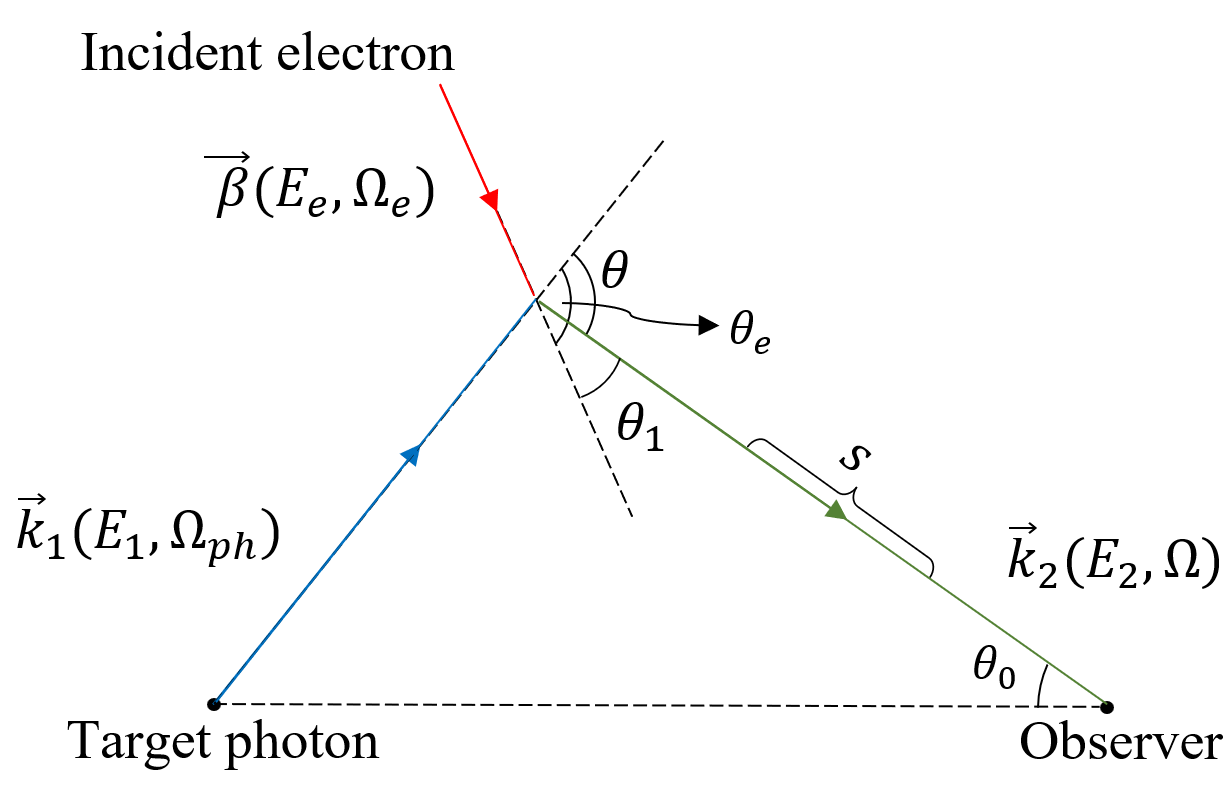
Figure 1: A schematic diagram that depicts the IC scattering for the case of a point source of target photons. $\vec{k}_{1}$, $\vec{k}_{2}$, and $\vec{\beta}$ are the directions of target photon, scattered photon and source electron. See the text for a detailed description of the variables. Note that in general $\vec{k}_{1}$, $\vec{k}_{2}$, and $\vec{\beta}$ do not lie in the same plane, see Fig. 2.

II.2 Assumptions

In general, the differential cross section Eq. 2 depends on many variables. To simplify, we assume a unidirectional target photon along direction $\Omega^{\prime}_{ph}$ from a point source, we also assume an isotropic distribution of source electron flux. That is:

$$\begin{split}f_{ph}&=\delta({\Omega_{ph}-\Omega^{\prime}_{ph}})\,,\\ f_{e}&=\frac{1}{4\pi}\,.\end{split}$$ (4)

Eq. 2 then becomes:

$$\left<\frac{d^{2}\sigma}{d\Omega dE_{2}}\right>=\frac{1}{4\pi}\int d\Omega_{e}\frac{d^{2}\sigma^{\prime}}{d\Omega dE_{2}}(E_{1},E_{2},E_{e},\Omega,\Omega_{e}),$$ (5)

where $\Omega_{ph}$ is dropped by the delta function and $\Omega_{e}$ is now defined w.r.t to the direction of target photon. The explicit form of the differential cross section in Eq. 3 is given by Jauch and Rohrlich (2012):

$$\frac{d^{2}\sigma^{\prime}}{d\Omega dE_{2}}=\frac{r_{e}^{2}\bar{X}}{2\gamma^{2}(1-\beta\cos\theta_{e})}\frac{E_{2}^{2}}{E_{1}^{2}}\delta(E_{2}-\bar{E}_{2}),$$ (6)

where $r_{e}$ is the classical electron radius, $\gamma$ is the electron Lorentz factor and

$$\bar{X}=\left[\frac{\kappa_{1}}{\kappa_{2}}+\frac{\kappa_{2}}{\kappa_{1}}+2m_{e}^{2}\left(\frac{1}{\kappa_{1}}-\frac{1}{\kappa_{2}}\right)+m_{e}^{4}\left(\frac{1}{\kappa_{1}}-\frac{1}{\kappa_{2}}\right)^{2}\right],$$ (7)

where $\kappa_{1}=p\cdot k_{1}=p_{0}k_{0}-\vec{p}\cdot\vec{k}_{1}$ and $\kappa_{2}=p\cdot k_{2}$ are the dot products of four momentum of incident electron and incident/scattered photon, the subscript 0 denotes the time component. $\bar{E}_{2}$ can be found from conservation of 4-momentum:

$$\bar{E}_{2}=\frac{E_{1}(1-\beta\cos\theta_{e})}{\frac{E_{1}}{E_{e}}(1-\cos\theta)+1-\beta\cos\theta_{1}},$$ (8)

where $\theta_{1}$ is the angle between source electron and scattered photon,

$$\cos\theta_{1}=\cos\theta\cos\theta_{e}+\sin\theta\sin\theta_{e}\cos(\phi_{e}-\phi).$$ (9)

We note that although Eq. 9 depends on 4 angular variables $\phi_{e},\theta_{e},\phi,\theta$, the two polar angles only come in as their difference $\phi_{e}-\phi$. This implies a polar symmetry on $\phi$ as we integrate $\phi_{e}$. In other words, Eq. 6 does not depend on the $\phi$, and we chose $\phi=0$ hereafter.

In the limit $\beta\ll 1$, Eq. 8 reduces to the Compton scattering formula and $\kappa_{1},\kappa_{2}$ become $m_{e}E_{1}$ and $m_{e}E_{2}$. Putting these expressions back in Eq. 6 yields the Klein-Nishina (KN) differential cross section in electron-rest frame (ERF):

$$\frac{d^{2}\sigma^{\prime}_{\text{KN}}}{d\Omega dE_{2}}=\frac{r_{e}^{2}}{2}\frac{E_{2}^{2}}{E_{1}^{2}}\left(\frac{E_{2}}{E_{1}}+\frac{E_{1}}{E_{2}}-\sin^{2}\theta\right)\delta(E_{2}-\bar{E}_{2}).$$ (10)

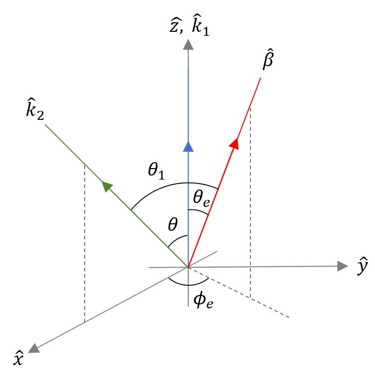
Figure 2: A diagram for the IC scattering between a photon and an electron. With the assumptions made in Eq. 4, we can choose to align the target photon direction with $+z-$axis and set $x-z$ plane as the scattering plane.

II.3 Reduction to MS result

As mentioned in the introduction, MS Moskalenko and Strong (2000) adopted an ultrarelativistic assumption, in particular, $\gamma\gg 1$ and $\theta_{1}=0$. The latter implies that scattered photons are unidirectional along the direction of electron, or $\Omega=\Omega_{e}$. To illustrate the effect of such approximation, we first rewrite the delta function in Eq. 6 as:

$$\delta(E_{2}-\bar{E}_{2})=\frac{\delta(\Omega_{e}-\Omega_{e,sol})}{\left|\frac{d\bar{E}_{2}}{d\Omega_{e}}\right|},$$ (11)

where $\Omega_{e,sol}$ is the solution to the condition of $E_{2}=\bar{E}_{2}(\Omega_{e,sol})$. The unidirectional approximation is then equivalent to:

$$\delta(\Omega_{e}-\Omega_{e,sol}) =\delta(\phi_{e})~{}\delta(\cos\theta_{e}-\cos\theta)$$ (12)

With this simplification, integration in Eq. 5 implies removing the $\Omega_{e}$ dependence and evaluate the denominator in Eq. 11 at $\Omega_{e}=\Omega$. By restoring a general source photon distribution $f_{ph}$ and integrating over $\Omega_{ph}$, it can be shown that the whole expression reduces to MS’s Eq. (8)Moskalenko and Strong (2000):

$$\left<\frac{d\sigma}{dE_{2}}\right>=\frac{\pi r_{e}^{2}}{E_{1}(\gamma-E_{2})^{2}}\int d\Omega_{ph}f_{ph}\left[2-2\frac{E_{2}}{\gamma}\left(\frac{1}{E^{\prime}_{1}}+2\right)\right.$$

$$\left.+\frac{E_{2}^{2}}{\gamma^{2}}\left(\frac{1}{{E^{\prime}}_{1}^{2}}+2\frac{1}{E^{\prime}_{1}}+3\right)-\frac{E_{2}^{3}}{\gamma^{3}}\right].$$ (13)

II.4 General treatment without unidirectional approximation

Instead of doing the unidirectional approximation in the last section, we look for the exact solution of $\cos\theta_{e,sol}$ in terms of $E_{1},E_{2},E_{e},\theta$ and $\phi_{e}$. To begin with, we write the complete form of Eq. 5 using Eq. 6, 7 and 11:

$$\left<\frac{d^{2}\sigma}{d\Omega dE_{2}}\right>$$

$$= \frac{r^{2}_{e}}{8\pi\gamma^{2}}\int d\Omega_{e}\frac{\bar{X}E^{2}_{2}}{(1-\beta\cos\theta_{e})E^{2}_{1}}\frac{\delta(\cos\theta_{e}-\cos\theta_{e,sol})}{\left|\frac{d\bar{E}_{2}}{d\cos\theta_{e}}\right|_{\cos\theta_{e,sol}}}$$

$$= \frac{r^{2}_{e}}{8\pi\gamma^{2}}\int^{2\pi}_{0}d\phi_{e}\sum_{\cos\bar{\theta}_{e,sol}}\left[\frac{\bar{X}E^{2}_{2}}{(1-\beta\cos\theta_{e})E^{2}_{1}\left|\frac{d\bar{E}_{2}}{d\cos\theta_{e}}\right|}\right]\,,$$

where

$$\frac{d\bar{E}_{2}}{d\cos\theta_{e}}$$

$$= \frac{\beta\bar{E}_{2}}{1-\beta\cos\theta_{e}}\left[\frac{\bar{E}_{2}}{E_{1}}(\cos\theta-\sin\theta\cos\phi_{e}\cot\theta_{e})-1\right].$$

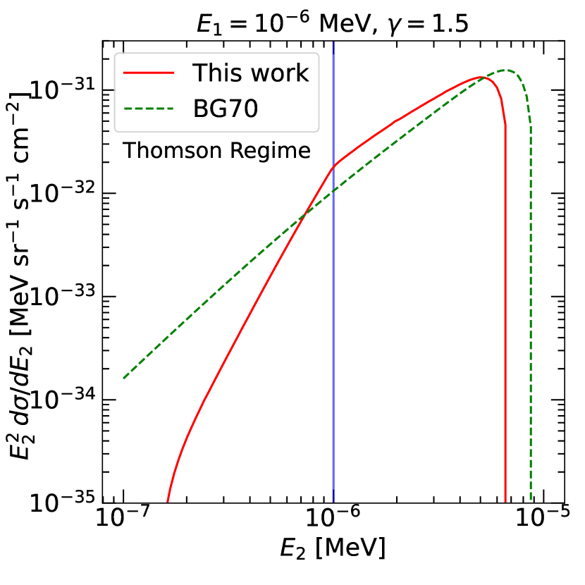
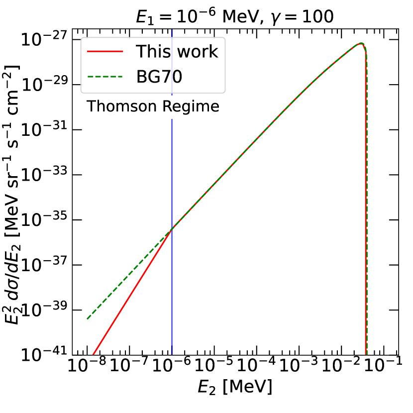
Figure 3: The differential cross sections $E_{2}^{2}\>d\sigma/dE_{2}$ against scattered photon energy $E_{2}$ in the Thomson regime $E_{1}\ll E_{e}$ (Sec. III.1.1). Left: target photon energy $E_{1}=10^{-6}$ MeV, source electron Lorentz factor $\gamma=1.5$. BG70 refers to the Eq. (2.48) in BLUMENTHAL and GOULD (1970), the blue line marks the value of $E_{1}$. See paragraph for more details; Right: target photon energy $E_{1}=10^{-6}$ MeV, source electron Lorentz factor $\gamma=100$.

The problem of finding the differential cross section then reduces to summing and finding the possible solutions $\cos\theta_{e,sol}$, and then numerically integrate over $\phi_{e}$. It can be achieved by putting Eq. 8 into a quadratic equation of $\tan(\theta_{e}/2)$:

$$(C-A)\tan^{2}\left(\frac{\theta_{e}}{2}\right)+2B\tan\left(\frac{\theta_{e}}{2}\right)+(C+A)=0,$$ (16)

where $A,B$ and $C$ are given by:

$$\begin{split}A&=\beta(E_{1}-E_{2}\cos\theta)\,,\\ B&=-E_{2}\beta\sin\theta\cos\phi_{e}\,,\\ C&=\frac{E_{2}E_{1}(1-\cos\theta)}{E_{e}}+E_{2}-E_{1}.\end{split}$$ (17)

Hence, the two solutions to the equation

$$\tan(\theta_{e}/2)=\frac{-B\pm\sqrt{A^{2}+B^{2}-C^{2}}}{C-A}$$ (18)

correspond to two possible IC scattering geometry for a given set of $(E_{2},E_{1},E_{e},\theta,\phi_{e})$. Although both solutions lead to physical scattering geometries, only positive solutions are retained. That is because a negative $\tan(\theta_{e}/2)$ can be mapped to a positive one $\theta_{e}\rightarrow\theta_{e}+\pi$ together with $\phi_{e}\rightarrow\phi_{e}+\pi$. Therefore, it represents a duplicated a solution at another $\phi_{e}$. The relation between a positive determinant $A^{2}+B^{2}-C^{2}$ and the physical limit of $E_{2}$ is explained in Appendix A.

III Results

III.1 Scattering between isotropic photon and isotropic electrons

In this section, we compare the results obtained with our general formalism to that from BG70 BLUMENTHAL and GOULD (1970), which was obtained using the high-$\gamma$ approximation and is used frequently in the IC literature.

BG70 also assumed isotropic photon and electron distributions. To match that, we evaluate the differential cross section by averaging over the scattering angle of Eq. II.4. Although Eq. II.4 is derived from isotropic source electron and unidirectional target photon (Eq. 4), averaging over the scattering angle is equivalent to averaging over the incident photon directions, and thus corresponds to an isotropic source photon distribution.

We note that in the context of thermal SZ effect, Sarkar et. al. Sarkar et al. (2019) also considered general isotropic scatterings. They defined the kinematic regimes by comparing the source photon energy $E_{1}$ and the electron energy $E_{e}$. This is different from us, as we consider mainly the energies in the electron-rest frame (ERF). Below we refer to primed variables as ERF quantities (e.g., $E_{1}^{\prime}$) and unprimed variables as the observer frame quantities (e.g., $E_{1}$).

III.1.1 Thomson regime ($E_{1}^{\prime}\ll m_{e}$)

When the ERF target photon energy $E_{1}^{\prime}=\gamma E_{1}(1-\beta\cos\theta_{e})$ is much smaller than the electron rest mass, the scattering between target photons and electrons falls into the Thomson regime regardless of the value of $\gamma$. In the Thomson limit, photon energies are the same before and after scattering in the ERF, $E_{1}^{\prime}\approx E_{2}^{\prime}$. In the ultrarelativistic limit ($\gamma\gg 1$), the maximum cutoff of the IC scattered photon energy in the observer frame, $E_{2,\rm max}$, is well approximated by $4\gamma^{2}E_{1}$, which is the limit used by BG70.

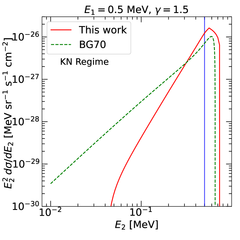
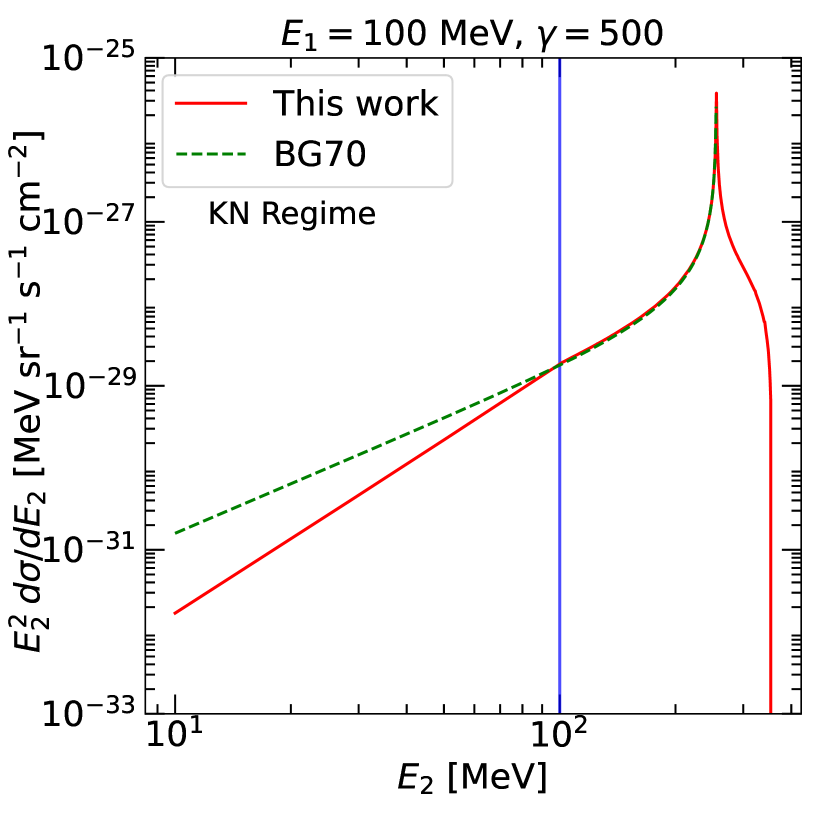
Figure 4: Similar to Fig. 3, but for the KN regime, $E^{\prime}_{1}\gtrsim m_{e}$, $E_{1}\lesssim E_{e}$ (Sec. III.1.2). Left: $E_{1}=0.5$ MeV and $\gamma=1.5$, which corresponds to mildly-relativistic scattering; Right: $E_{1}=100$ MeV and $\gamma=500$, which corresponds to ultrarelativistic scattering.

Our exact formalism is expected to agree well with BG70 in the ultrarelativistic limit. However, in the mildly-relativistic limit, when the $\gamma$ value is smaller, the approximation $E_{2,\rm max}\sim 4\gamma^{2}E_{1}$ from head-on scattering between source electron and photon no longer holds. In this case, the upscattered photon energy

$$E_{2}\simeq\frac{1-\beta\cos\theta_{e}}{1-\beta\cos\theta_{1}}E_{1}$$ (19)

can be obtained by taking the limit $E_{1}\ll E_{e}$ in Eq. 8 or by considering the relation $E_{1}^{\prime}=E_{2}^{\prime}$ and express $E_{1}^{\prime},E_{2}^{\prime}$ in observer frame quantities. The exact $E_{2,\rm max}$ is then yielded by maximizing Eq. 19 with respect to $\theta_{e}$ and $\theta_{1}$.

The left panel in Fig. 3 plots the differential cross section against $E_{2}$ for the mildly-relativistic case of $\gamma=1.5$ electrons scattering with source photons at $10^{-6}$ MeV. The scattering falls into the Thomson regime as $E_{1}^{\prime}\approx 3\times 10^{-6}$ MeV. The blue line marks the value of $E_{1}$ and separates the spectrum into upscattering ($E_{1}<E_{2}$) and downscattering ($E_{1}>E_{2}$) regions. In our exact calculation, the cutoff energy is lower than BG70, and the differential cross section shifts to the left. Our differential cross section also differs from BG70 in the down-scattering region, which we discuss in detail later in Sec. III.1.4.

The right panel of Fig. 3 shows the same plot but with $\gamma=100$ for source electrons to depict the ultrarelativistic IC scattering. The scattering is still in the Thomson regime as $E_{1}^{\prime}\sim 2\times 10^{-3}$ MeV $\ll m_{e}$. As expected, in the upscattering domain $E_{2}>E_{1}$, our result agrees well with BG70, and have produced the same $E_{2,\rm max}=4\gamma^{2}E_{1}\approx 4\times 10^{-2}$ MeV. In addition, the total Thomson cross section $\sigma_{T}=8\pi/3~{}r_{e}^{2}$ can be recovered by integrating the area under $d\sigma/dE_{2}$ in Fig. 3 over $E_{2}$. Therefore, it validates our formalism on the differential cross section in the ultrarelativistic limit.

III.1.2 KN regime ($E_{1}\lesssim E_{e}$, $E^{\prime}_{1}\gtrsim m_{e}$)

For larger values of $E_{1}$ that approaches $E_{e}$, the ERF target photon energy $E_{1}^{\prime}$ can easily surpass the rest mass of the electron $m_{e}$; this corresponds to the KN regime. In this regime, BG70 approximated the maximum scattered photon energy $E_{2,\rm max}$ to be:

$$E_{2,\rm max}\approx\frac{4\gamma^{2}E_{1}}{1+4\gamma\frac{E_{1}}{m_{e}}}\,,$$ (20)

which follows from applying the large $\gamma$, head-on scattering with the photon scattered backward approximation ($\theta_{e}=\pi,\theta_{1}=0$) to the conservation of energy Eq. 8. When $E_{1}^{\prime}\gg m_{e}$, the term $4\gamma E_{1}/m_{e}$ in the denominator of Eq. 20 dominates and $E_{2,\rm max}\simeq E_{e}$. Using the general differential cross section, we instead find that $E_{2,\rm max}=(\gamma-1)E_{e}+E_{1}$, which is simply the case when the electron transfer all its kinetic energy to the photon and is valid for any values of $\gamma$.

The left panel in Fig. 4 shows the differential cross section of $\gamma=1.5$ electrons scattering with 0.5 MeV target photons. As $E_{1}^{\prime}\approx 2\gamma E_{1}=1.5$ MeV, which implies that photons undergo Compton scattering in ERF and a large portion of the energy is transferred to the electron. This corresponds to the KN regime.

The right panel in Fig. 4 shows the ultrarelativistic scattering $\gamma=500$ electron and 100 MeV target photons, which is in the regime of $E_{1}^{\prime}\approx 2\gamma E_{1}\gg m_{e}$. As expected, our results agree with BG70 in the $E_{1}<E_{2}<E_{e}$ energy range. BG70’s formula, however, does not work above $E_{e}$, while our results extend correctly to the true maximum at $E_{2}=(\gamma-1)E_{e}+E_{1}$. We note that for large $\gamma$ cases, the differential cross section strongly peaks at the electron energy $E_{e}$. This can be clearly seen in this plot (as well as in the right panel of Fig. 5.)

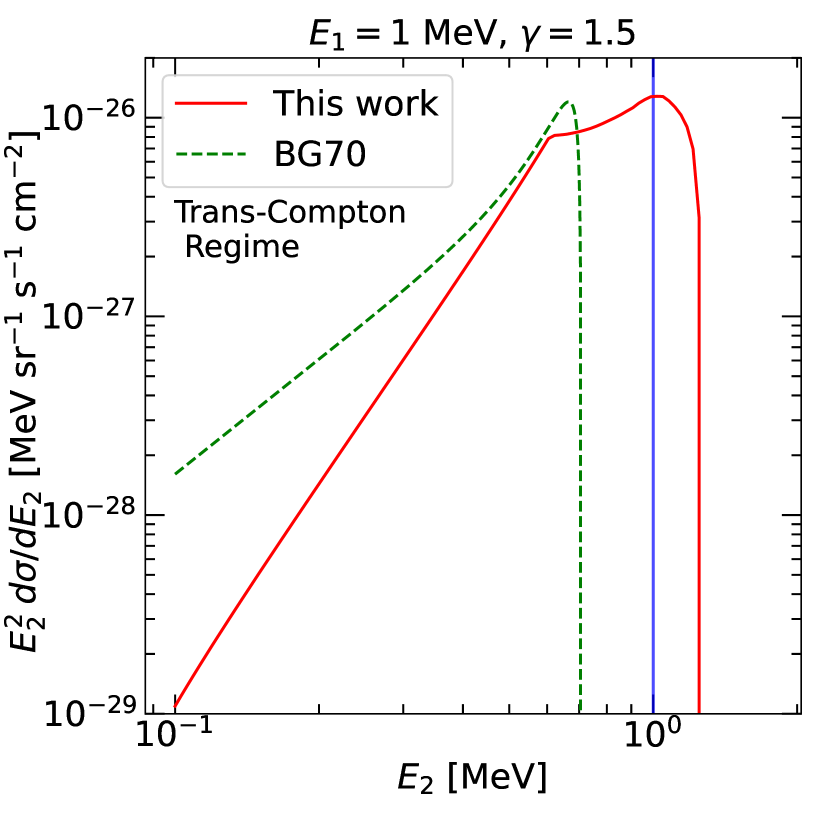
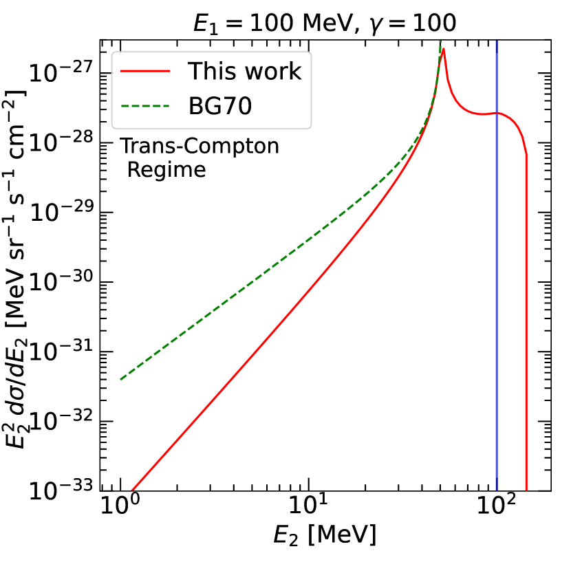
Figure 5: Similar to Fig. 3, but for the trans-Compton regime, $E_{1}>E_{e}$ (Sec. III.1.3). Left: $E_{1}=1$ MeV, $\gamma=1.5$, corresponds to mildly-relativistic scattering; Right: $E_{1}=100$ MeV, $\gamma=100$, corresponds to ultrarelativistic scattering.

III.1.3 Trans-Compton regime ($E_{1}>E_{e}$)

When $E_{1}>E_{e}$, that is, when the target photon energy is greater than the electron energy, the scattering in ERF entirely falls in the KN regime. But in this case, the target photon mostly experiences energy loss, similar to the case of Compton scattering. Although the case of $E_{1}>E_{e}$ was not considered in BG70, we compare to their formula for completeness. Our formalism works for all energy range up to $E_{2,\rm max}=E_{1}+(\gamma-1)E_{e}$.

The left panel in Fig. 5 shows the differential cross section of $\gamma=1.5$ electrons scattering with 1 MeV target photons, which corresponds to a mildly-relativistic scattering. The ultrarelativistic case ($\gamma=100$, $E_{1}=100$ MeV) is illustrated in the right panel of Fig. 5. The large deviation of BG70’s differential cross section from ours implies the breakdown of ultrarelativistic approximation in this kinematic regime.

III.1.4 Down-scattering cases ($E_{2}<E_{1}$)

In all the cases discussed above, our general formalism includes the effect of down scattering (when $E_{2}<E_{1}$), which is not included in BG70. From Fig. 3 to Fig. 5, we note that the correct differential cross sections always decline more rapidly than BG70 in the down scattering regime. In addition, we also correctly calculate the minimum scattered photon energy $E_{2,\rm min}$ using Eq. 8, which corresponds to a photon and an electron initially travelling in the same direction with the photon scattered backward ($\theta_{e}=0,~{}\theta_{1}=\pi$). In contrast, there is no $E_{2,\rm min}$ from BG70.

IV Case studies

We consider two simple cases of high-energy IC emission to show that our formalism can correctly reproduce the results in ultrarelativistic limits, and find the regime where the ultrarelativistic assumption would break down.

IV.1 Solar Inverse Compton Emission

Solar IC emission are produced when cosmic-ray electrons up scatter solar photons Moskalenko et al. (2006); Orlando et al. (2008); Orlando and Strong (2007, 2008). The anisotropic IC scattering cross section in MS Moskalenko and Strong (2000) (with ultrarelativistic approximations) was adopted to produce the IC emission package StellarICs Orlando and Strong (2013). In this section, we compare our exactly formalism with the latest StellarICs calculation on solar gamma ray in Ref. Orlando and Strong (2021).

Fig. 6 shows the LOS solar IC spectral intensity from the general electron-photon scattering formalism and StellarICs. The computation of our spectrum follows the master equation Eq. 1 with an observation angle $\theta_{0}=0.3^{\circ}$. We employ the same $n_{ph},f_{ph},n_{e},f_{e}$ as in StellarICs. Specifically, the differential number density of target photons follows a black-body spectrum at 5770 K, with a spherical and uniform distribution. The differential number density of source electrons is inferred from the curve fitted with AMS02 data in the Fig. 3 of  Orlando and Strong (2021) and the distribution is isotropic. From Fig. 6, our spectrum agrees well with StellarICs in the range of $E_{2}=10^{-2}-10^{3}$ MeV. The correction from releasing the ultrarelativistic approximation in the differential cross section cannot be seen in the figure, since electrons with $\gamma=10^{2}-10^{4}$ are responsible for scattering solar photons to the range of hard X-rays and gamma rays. The general formula thus reduces to ultrarelativistic approximation in this regime and converge to StellarICs’s.

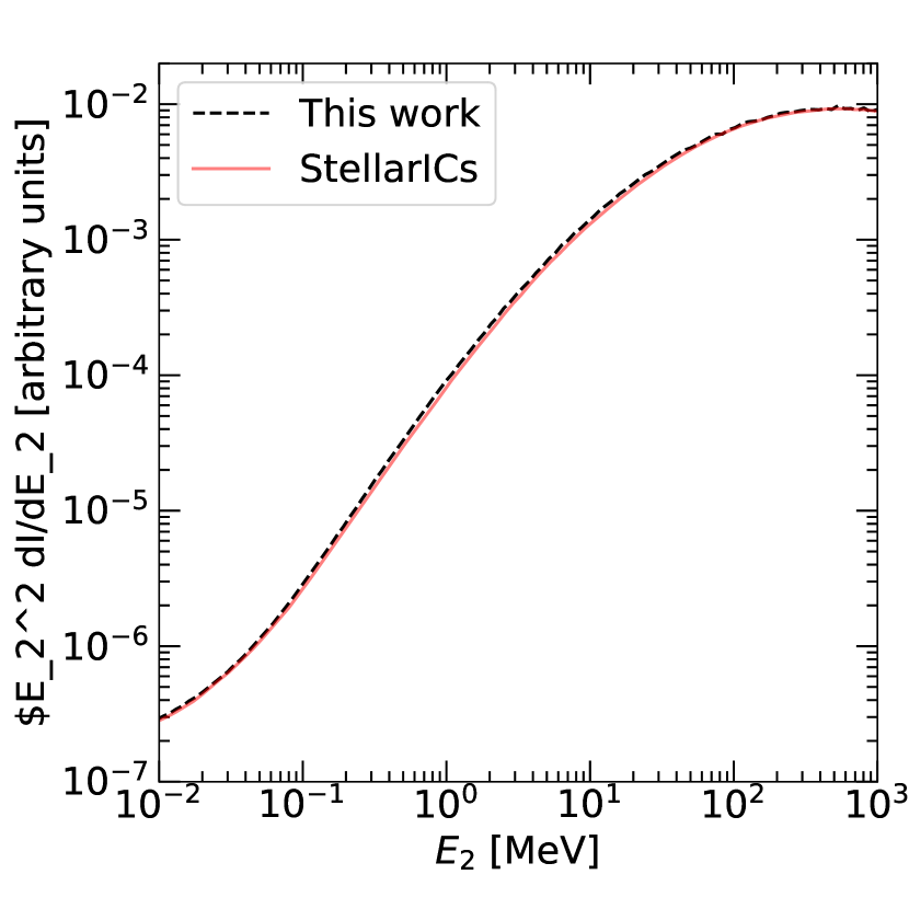
Figure 6: The LOS solar IC intensity at $0.3^{\circ}$ away from the centre of the sun. The red spectrum labelled with ’StellarICs’ refers to the solid blue curve in  Orlando and Strong (2021) Fig. 4. The intensity spectrum in this work was computed using Eq. 1 with the same solar photon and cosmic electron spectrum in  Aguilar et al. (2014). In particular, a thermal spectrum from $10^{-7}$ to $10^{-5}$ MeV was used for the photon field. An electron spectrum from $10^{1}$ to 10 ⁵ MeV that follows the curve fitted with AMS02 data in Fig. 3 of  Orlando and Strong (2021), was used.

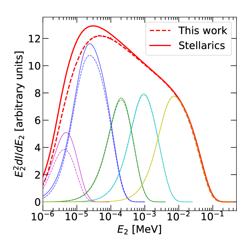
Figure 7: A decomposition of LOS solar IC spectrum. The decomposed spectra with $\gamma=1-1.5$, $\gamma=1.5-5$, $\gamma=5-10$, $\gamma=10-25$ and $\gamma=25-100$ are given by the magenta, blue, green, cyan, and yellow curves, respectively. Solid lines represent the StellarICs results and our results (general formalism) are shown in dashed lines. Linear vertical scale is used to highlight the mildly-relativistic correction.

For smaller values of $E_{2}$, we expect to see some discrepancies between our exact calculation and the ultrarelativistic approximations. For illustration, we extend the electron spectrum to lower energies, adopting a $E_{e}^{-3.2}$ power law between $\gamma=1$ to 100.

Fig. 7 shows the full energy range for the anisotropic solar IC scattering. It is clear that the solar emission above $E_{2}\approx 10^{-3}$ MeV is indeed dominated by larger $\gamma>10$. The ultrarelativistic approximation holds in this regime and the two emission spectra coincide. When $E_{2}<10^{-3}$ MeV, our calculation deviates from StellarICs. From the spectrum decomposition, we see the deviation is due to mildly-relativistic correction from general formalism. The deviation is the largest in the interval $\gamma=1.5-5$. The overall correction to the total emission is a reduced intensity for $E_{2}<5\times 10^{-3}$ MeV.

IV.2 Synchrotron Self-Compton

Synchrotron photons are emitted when energetic electrons gyrate along strong magnetic fields. These synchrotron photons can also undergo IC scattering with the gyrating electrons, resulting high-energy gamma-ray emission. This synchrotron self-Compton (SSC) mechanism have been used to model gamma-ray emissions from various sources, such as blazars and relativistic jets Potter and Cotter (2012); Inoue et al. (2019); Banik and Bhadra (2019).

In the SSC mechanism, the target photon energy is higher than the solar IC case. We therefore consider a simplified SSC model to see the effect of relaxing the ultrarelativistic assumption.

We consider a relativistic jet, where the Lorentz factor of the jet is 500 with a $0.5^{\circ}$ observation angle from the jet direction. The resulted boost from the jet frame (JF) to the observer frame is about 50. Both the electron and photon spectra are taken to be isotropic in JF so that we can compare the result with BG70. In the JF (quantities denoted with the “JF” subscript), we consider the electron spectrum to be a power law $E_{e,\text{JF}}^{-3}$ between $\gamma_{\text{JF}}=1$ to $10^{4}$. The photon spectrum is taken to be a $E_{1,\text{JF}}^{-2}$ power law between $10^{-3}$ MeV to $10^{3}$ MeV.

Fig. 8 shows the SSC emission spectrum $E_{2}^{2}d\epsilon/dE_{2}$ in the observer frame with the above configuration. The red dashed line represents the total emission from our calculation. For comparison, results obtained from BG70 is shown in solid lines. Our results agrees well to that obtained with BG70 at high photon energies, but large deviations start to appear at low energy.

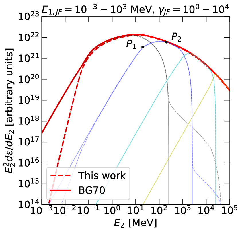
Figure 8: The SSC emission spectrum at observation angle $0.5^{\circ}$ away from the jet with $E_{1,\text{JF}}$ from $10^{-3}$ to $10^{3}$ MeV and $\gamma_{\text{JF}}$ from 1 to $10^{4}$. Both of target photons and electrons are assumed to be isotropic in JF. The emission is plotted in scattered photon energy in observer frame $E_{2}$. Red line gives the total emission. The individual contributions from $\gamma_{\text{JF}}=1-10^{1},10^{1}-10^{2},10^{2}-10^{3}$, and $10^{3}-10^{4}$ are presented in the black, blue, cyan, and yellow lines, respectively. The transition points $P_{1}$ and $P_{2}$ for the blue line are highlighted. See the text for details about the decomposition spectrum and transition points.

For $E_{2,\text{JF}}$ smaller than the minimum photon energy, $10^{-3}$ MeV ($E_{2}$ $\approx 0.05$ MeV, in Fig. 8), these are dominated by down-scattered photons produced in the Thomson regime. In this case, BG70’s formula corresponds to a flat differential cross section, and thus results in a $E_{2}^{2}$ behaviour in the $E_{2}^{2}d\epsilon/dE_{2}$ plot. As discussed in Sec. III.1.4, our results deviates considerably from the ultrarelativistic approximation.

To further illustrate the physics of the IC scattering, consider the blue line in Fig. 8, which is the spectrum produced by electrons with $\gamma_{\text{JF}}$ between $10^{1}$ and $10^{2}$. For $E_{2}>0.05$ MeV ($E_{2,\text{JF}}>10^{-3}$), the spectrum enters a region where all scattering geometries are accessible by Thomson scattering, thus resulting in the $E_{2}^{2}$ behaviour. The $E_{2}^{2}$ trend continues until reaching the point $P_{1}$, which corresponds to $E_{2,\text{JF}}=4\gamma_{\text{JF,m}}^{2}E_{1,\text{JF,m}}$, where both $\gamma_{\text{JF,m}}$ and $E_{1,\text{JF,m}}$ are the lower cutoff of the source photon and electron spectrum. Above $P_{1}$, the spectrum then softens mainly due to the spectral shape of source photons. Finally, above the point $P_{2}$, the scattering transits into the KN regime, and the spectrum steepens further mainly due to the spectral shape of source electrons. We note that the transition into the KN regime can be rapid in the case of large $\gamma$ values. E.g., for the case of the the yellow line in Fig. 8.

Finally, as mentioned in Sec. III.1.2, our formalism works correctly for cases with $E_{2}>E_{e,\rm{max}}$ when there are appreciable energy in the target photon. These contribution appears as the ’bump’ features in Fig. 8. In these cases, the extra contributions are overwhelmed by those from higher energy electrons.

V Conclusions and Outlook

In this work, we consider the scattering between energetic electrons and photons, and study the differential cross section for the outgoing photon spectrum. This process is frequently used in high-energy astrophysics for the production of IC photon emission.

We demonstrate that for the general case (without ultrarelativistic approximation) of anisotropic photons scattering with isotropic electrons, the differential cross section can be written as Eq. II.4, which can be easily integrated numerically by finding the analytic solutions to the scattering geometry, given by Eq. 18.

Focusing on isotropic photon and isotropic electron scatterings, we compare our formalism with that from BG70, which considered the ultrarelativistic approximation. We find that the scattering can be divided into three regimes, the Thomson regime, the KN regime, and the Trans-Compton regime. In general, we find that there would be deviations to the BG70 formula in the downscattering limit ($E_{2}<E_{1}$), as well as when the target photon energy becomes comparable to the electron energy.

To validate our formalism in the ultrarelativistic limit and show that it is numerically stable, we consider two cases of high-energy IC emission. The first is solar IC emission produced by anisotropic solar photon scattering with isotropic cosmic-ray electrons. We find that our results agree well with that from StellarICs Orlando and Strong (2021). Due to solar photons being relatively low in energy, corrections from the exact formalism only appear below keV photon energy. The second case we consider is SSC emission, where isotropic synchrotron photons can scatter with isotropic electrons in astrophysical jets. Due to the synchrotron photons being comparatively energetic, the corrections from downscattering can be significant in the low energy part of the SSC. At high energies, our results agree well with that produced by the BG70 formula.

In these case studies, although we only consider scattering between isotropic source electrons with isotropic photons (SSC) or anisotropic photons (solar IC), it is straightforward to generalise the calculations to include different angular distributions for photons and electrons in Eq. 2. For example, for the case of external Compton emission in astrophysical jets Dermer (1995); Kelner et al. (2014), photons emission are produced by jet electrons scattering with photons from CMB, accretion disk, or dusty torus Finke (2016). In these cases, both photon and electron distribution can be anisotropic, and thus a more general formalism like ours is required.

In this work, we have focused much of our discussion in the gamma-ray regime, where IC emission is typically considered. This is in part to show that our formalism can be reduced to the well established works in the ultrarelativistic regime. In general, we expect that a general formalism like this is required whenever mildly relativistic electrons are involved, or when the target photon energy is not small compared to electron energy.

Finally, through Eq. 18, we have obtained an exact solution to the scattering angle geometry. This allows us to obtain the photon polarization caused by anisotropic scattering, which we will discuss in detail in a followup work Lai and Ng . In the literature, results of photon polarization caused by IC scattering are somewhat inconsistent Krawczynski (2012). This work forms the basis for a numerical framework to obtain the polarization spectrum. This is especially timely, given that there are recent and future X-ray and gamma-ray telescopes that are capable of detecting photon polarizations Weisskopf et al. (2016); Zhang et al. (2016); Alessandro et al. (2021).

VI Acknowledgement

We thank Ming-Chung Chu for helpful discussions. This work makes use of StellarICs, an open source code that is available from Ref. Orlando and Strong (2021). This project is supported by a grant from the Research Grant Council of the Hong Kong Special Administrative Region, China (Project No. 24302721).

Appendix A Relating positive determinant to the kinematic constraint of $E_{2}$

A non-negative determinant in the quadratic equation Eq. 16 $\Delta=A^{2}+B^{2}-C^{2}\geq 0$ secures real solutions and sets the kinematic constraint on the possible range of $E_{2}$. To illustrate this, rewrite the determinant into a quadratic equation of $E_{2}$:

$$K_{1}E^{2}_{2}+K_{2}E_{2}+K_{3}\geq 0$$ (21)

$$K_{1} = \beta^{2}(\cos^{2}\theta+\sin^{2}\theta\cos^{2}\phi_{e})-\left[\frac{E_{1}(1-\cos\theta)}{E_{e}}+1\right]^{2}$$

$$K_{2} = 2E_{1}\left[\frac{E_{1}(1-\cos\theta)}{E_{e}}+1-\beta\cos\theta\right]$$

$$K_{3} = (\beta^{2}-1)E^{2}_{1}.$$

Eq. 21 has another determinant $\Delta^{\prime}=K_{2}^{2}-4K_{1}K_{3}$ which is positive definite for a physical solution. In the non-relativistic KN regime, $\beta\rightarrow 0$, $E_{1}\sim m_{e}\approx E_{e}$, We have $K_{1}<0$ such that $E_{2}$ is bounded the roots of Eq. 21. We also have $\Delta^{\prime}\approx 0$, so:

$$\frac{E_{1}}{\frac{E_{1}}{m_{e}}(1-\cos\theta)+1} \leq E_{2}\leq\frac{E_{1}}{\frac{E_{1}}{m_{e}}(1-\cos\theta)+1}$$ (22)

$$\implies E_{2} = \frac{E_{1}}{\frac{E_{1}}{m_{e}}(1-\cos\theta)+1}=E_{\text{Compton}}\,,$$

as expected.

In the Thomson regime, $E^{\prime}_{1}\ll m_{e}$ and $E_{2}$ is again bounded by the roots as $K_{1}<0$. We further consider ultrarelativistic limit such that $\gamma\ll 1$, both maximum and minimum scattered photon energy $E_{2}$ occurs at $\cos\theta=-1$ scattering in this limit. Manipulation on $\Delta^{\prime}$ yields:

$$\begin{split}K^{2}_{2}-4K_{1}K_{3}&=(1+\beta)^{2}-(1-\beta^{2})^{2}\\ &=(1+\beta)^{2}[1-(1-\beta)^{2}]\\ &\approx(1+\beta)^{2}\left(1-\frac{1}{4\gamma^{4}}\right),\end{split}$$ (23)

where the relativistic approximation $\beta\approx 1-1/(2\gamma^{2})$ is used in last line. With Eq. 23 and additional calculations, the conditional $\Delta\geq 0$ becomes:

$$\frac{(1-(1-1/(8\gamma^{4}))}{1-\beta}E_{1}\leq E_{2} \leq\frac{1+(1-1/(8\gamma^{4}))}{1-\beta}E_{1}$$

$$\frac{1}{4\gamma^{2}}E_{1}\leq E_{2} \leq 4\gamma^{2}E_{1}.$$ (24)

Again, it agrees with the limits mentioned in Rybicki and Lightman (1986). Therefore, a real solution of Eq. 18 implies a physical solution for the scattering.

References

- Hunter et al. (1997) S. D. Hunter et al., “EGRET observations of the diffuse gamma-ray emission from the galactic plane,” Astrophys. J. 481, 205–240 (1997).
- Moskalenko and Strong (1999) I. V. Moskalenko and A. W. Strong, “Puzzles of Galactic continuum gamma-rays,” Astrophysical Letters and Communications 38, 445–448 (1999), arXiv:astro-ph/9811221 [astro-ph] .
- Strong et al. (2000) Andrew W. Strong, Igor V. Moskalenko, and Olaf Reimer, “Diffuse Continuum Gamma Rays from the Galaxy,” ApJ 537, 763–784 (2000), arXiv:astro-ph/9811296 [astro-ph] .
- Thompson et al. (1997) D. J. Thompson, D. L. Bertsch, D. J. Morris, and R. Mukherjee, “Energetic gamma ray experiment telescope high-energy gamma ray observations of the Moon and quiet Sun,” J. Geophys. Res. 102, 14735–14740 (1997).
- Strong et al. (2004a) Andrew W. Strong, Igor V. Moskalenko, and Olaf Reimer, “Diffuse galactic continuum gamma rays: A model compatible with EGRET data and cosmic-ray measurements,” The Astrophysical Journal 613, 962–976 (2004a).
- Strong et al. (2004b) Andrew W. Strong, Igor V. Moskalenko, and Olaf Reimer, “A new determination of the extragalactic diffuse gamma-ray background from EGRET data,” The Astrophysical Journal 613, 956–961 (2004b).
- Ackermann et al. (2011) M. Ackermann et al., “A Cocoon of Freshly Accelerated Cosmic Rays Detected by Fermi in the Cygnus Superbubble,” Science 334, 1103–1107 (2011).
- Orlando and Strong (2007) E. Orlando and A. W. Strong, “Gamma rays from halos around stars and the sun,” Astrophysics and Space Science 309, 359–363 (2007).
- Moskalenko et al. (2006) Igor V. Moskalenko, Troy A. Porter, and Seth W. Digel, “Inverse Compton Scattering on Solar Photons, Heliospheric Modulation, and Neutrino Astrophysics,” ApJ 652, L65–L68 (2006), arXiv:astro-ph/0607521 [astro-ph] .
- Zhou et al. (2017) Bei Zhou, Kenny C. Y. Ng, John F. Beacom, and Annika H. G. Peter, “TeV solar gamma rays from cosmic-ray interactions,” Physical Review D 96 (2017), 10.1103/physrevd.96.023015.
- Orlando and Strong (2008) E. Orlando and A. W. Strong, “Gamma-ray emission from the solar halo and disk: a study with EGRET data,” A&A 480, 847–857 (2008), arXiv:0801.2178 [astro-ph] .
- Orlando et al. (2008) E. Orlando, D. Petry, and A. W. Strong, “Extended inverse-Compton gamma-ray emission from the Sun seen by EGRET,” in International Cosmic Ray Conference, International Cosmic Ray Conference, Vol. 1 (2008) pp. 11–14.
- Abdo et al. (2011) A. A. Abdo et al. (Fermi-LAT), “Fermi-LAT Observations of Two Gamma-Ray Emission Components from the Quiescent Sun,” Astrophys. J. 734, 116 (2011), arXiv:1104.2093 [astro-ph.HE] .
- Ng et al. (2016) Kenny C. Y. Ng, John F. Beacom, Annika H. G. Peter, and Carsten Rott, “First observation of time variation in the solar-disk gamma-ray flux with fermi,” Physical Review D 94 (2016), 10.1103/physrevd.94.023004.
- Orlando and Strong (2021) Elena Orlando and Andrew Strong, “StellarICS: inverse Compton emission from the quiet Sun and stars from keV to TeV,” J. Cosmology Astropart. Phys 2021, 004 (2021), arXiv:2012.13126 [astro-ph.HE] .
- Tang et al. (2018) Qing-Wen Tang, Kenny C. Y. Ng, Tim Linden, Bei Zhou, John F. Beacom, and Annika H. G. Peter, “Unexpected dip in the solar gamma-ray spectrum,” Phys. Rev. D 98, 063019 (2018), arXiv:1804.06846 [astro-ph.HE] .
- Linden et al. (2022) Tim Linden, John F. Beacom, Annika H. G. Peter, Benjamin J. Buckman, Bei Zhou, and Guanying Zhu, “First observations of solar disk gamma rays over a full solar cycle,” Phys. Rev. D 105, 063013 (2022), arXiv:2012.04654 [astro-ph.HE] .
- Linden et al. (2018) Tim Linden, Bei Zhou, John F. Beacom, Annika H. G. Peter, Kenny C. Y. Ng, and Qing-Wen Tang, “Evidence for a New Component of High-Energy Solar Gamma-Ray Production,” Phys. Rev. Lett. 121, 131103 (2018), arXiv:1803.05436 [astro-ph.HE] .
- Chiang and Dermer (1999) J. Chiang and C. D. Dermer, “Synchrotron and ssc emission and the blast-wave model of gamma-ray bursts,” Astrophys. J. 512, 699 (1999), arXiv:astro-ph/9803339 .
- Meszaros et al. (1994) P. Meszaros, M. J. Rees, and H. Papathanassiou, “Spectral properties of blast wave models of gamma-ray burst sources,” Astrophys. J. 432, 181–193 (1994), arXiv:astro-ph/9311071 .
- Yuksel et al. (2009) Hasan Yuksel, Matthew D. Kistler, and Todor Stanev, “TeV Gamma Rays from Geminga and the Origin of the GeV Positron Excess,” Phys. Rev. Lett. 103, 051101 (2009), arXiv:0810.2784 [astro-ph] .
- Linden et al. (2017) Tim Linden, Katie Auchettl, Joseph Bramante, Ilias Cholis, Ke Fang, Dan Hooper, Tanvi Karwal, and Shirley Weishi Li, “Using HAWC to discover invisible pulsars,” Phys. Rev. D 96, 103016 (2017), arXiv:1703.09704 [astro-ph.HE] .
- Sudoh et al. (2019) Takahiro Sudoh, Tim Linden, and John F. Beacom, “TeV Halos are Everywhere: Prospects for New Discoveries,” Phys. Rev. D 100, 043016 (2019), arXiv:1902.08203 [astro-ph.HE] .
- Sunyaev and Zeldovich (1970) R. A. Sunyaev and Ya. B. Zeldovich, “Small scale fluctuations of relic radiation,” Astrophys. Space Sci. 7, 3–19 (1970).
- Jones (1968) F C Jones, “Calculated spectrum in inverse-compton-scattered photons.” Phys. Rev., 167: 1159-69(Mar. 25, 1968). (1968), 10.1103/PhysRev.167.1159.
- BLUMENTHAL and GOULD (1970) GEORGE R. BLUMENTHAL and ROBERT J. GOULD, “Bremsstrahlung, synchrotron radiation, and compton scattering of high-energy electrons traversing dilute gases,” Rev. Mod. Phys. 42, 237–270 (1970).
- Rybicki and Lightman (1986) George B. Rybicki and Alan P. Lightman, Radiative Processes in Astrophysics (1986).
- Inoue et al. (2019) Yoshiyuki Inoue, Dmitry Khangulyan, Susumu Inoue, and Akihiro Doi, “On high-energy particles in accretion disk coronae of supermassive black holes: implications for MeV gamma rays and high-energy neutrinos from AGN cores,” (2019), 10.3847/1538-4357/ab2715, arXiv:1904.00554 [astro-ph.HE] .
- Banik and Bhadra (2019) Prabir Banik and Arunava Bhadra, “Describing correlated observations of neutrinos and gamma-ray flares from the blazar TXS 0506+056 with a proton blazar model,” Phys. Rev. D 99, 103006 (2019), arXiv:1908.11849 [astro-ph.HE] .
- Takami et al. (2014) Hajime Takami, Koutarou Kyutoku, and Kunihito Ioka, “High-Energy Radiation from Remnants of Neutron Star Binary Mergers,” Phys. Rev. D 89, 063006 (2014), arXiv:1307.6805 [astro-ph.HE] .
- Belmont (2009) R. Belmont, “Numerical computation of isotropic Compton scattering,” Astron. Astrophys. 506, 589 (2009), arXiv:0908.2705 [astro-ph.HE] .
- Nagirner and Poutanen (1994) D. I. Nagirner and J. Poutanen, Single Compton scattering, Vol. 9 (1994).
- Pe’er and Waxman (2005) Asaf Pe’er and Eli Waxman, “Time dependent numerical model for the emission of radiation from relativistic plasma,” Astrophys. J. 628, 857–866 (2005), arXiv:astro-ph/0409539 .
- Coppi and Blandford (1990) P S Coppi and R D Blandford, “Reaction rates and energy distributions for elementary processes in relativistic pair plasmas,” Monthly Notices of the Royal Astronomical Society 245, 453–453 (1990), https://academic.oup.com/mnras/article-pdf/245/3/453/42466511/mnras0453.pdf .
- Pe’er et al. (2006) Asaf Pe’er, Peter Meszaros, and Martin J. Rees, “The observable effects of a photospheric component on grb’s and xrf’s prompt emission spectrum,” Astrophys. J. 642, 995–1003 (2006), arXiv:astro-ph/0510114 .
- Vurm and Poutanen (2009) Indrek Vurm and Juri Poutanen, “Time-dependent modelling of radiative processes in hot magnetized plasmas,” Astrophys. J. 698, 293–316 (2009), arXiv:0807.2540 [astro-ph] .
- Sarkar et al. (2019) Abir Sarkar, Jens Chluba, and Elizabeth Lee, “Dissecting the Compton scattering kernel I: Isotropic media,” Mon. Not. Roy. Astron. Soc. 490, 3705–3726 (2019), arXiv:1905.00868 [astro-ph.CO] .
- Aharonian and Atoyan (1981) F. A. Aharonian and A. M. Atoyan, “Compton Scattering of Relativistic Electrons in Compact X-Ray Sources,” Ap&SS 79, 321–336 (1981).
- Chen and Bastian (2012) Bin Chen and Timothy S. Bastian, “The Role of Inverse Compton Scattering in Solar Coronal Hard X-ray and Gamma-ray Sources,” Astrophys. J. 750, 35 (2012), arXiv:1108.0131 [astro-ph.SR] .
- Murase et al. (2010) Kohta Murase, Kenji Toma, Ryo Yamazaki, Shigehiro Nagataki, and Kunihito Ioka, “High-energy emission as a test of the prior emission model for gamma-ray burst afterglows,” MNRAS 402, L54–L58 (2010), arXiv:0910.0232 [astro-ph.HE] .
- Nagirner and Poutanen (1993) D. I. Nagirner and Yu. J. Poutanen, “Compton scattering by Maxwellian electrons - Redistribution of radiation according to frequencies and directions,” Astronomy Letters 19, 262–267 (1993).
- Brunetti (2000) G. Brunetti, “Anisotropic inverse Compton scattering from the trans-relativistic to the ultrarelativistic regime and application to the radio galaxies,” Astropart. Phys. 13, 107–125 (2000), arXiv:astro-ph/9908236 .
- Poutanen and Vurm (2010) Juri Poutanen and Indrek Vurm, “Theory of Compton scattering by anisotropic electrons,” Astrophys. J. Suppl. 189, 286–308 (2010), arXiv:1006.2397 [astro-ph.HE] .
- Kelner et al. (2014) S. R. Kelner, E. Lefa, F. M. Rieger, and F. A. Aharonian, “The Beaming Pattern of External Compton Emission from Relativistic Outflows: The Case of Anisotropic Distribution of Electrons,” ApJ 785, 141 (2014), arXiv:1308.5157 [astro-ph.HE] .
- Molnar and Birkinshaw (1999) S. M. Molnar and M. Birkinshaw, “Inverse Compton scattering in mildly relativistic plasma,” Astrophys. J. 523, 78 (1999), arXiv:astro-ph/9903444 .
- Moskalenko and Strong (2000) Igor V. Moskalenko and Andrew W. Strong, “Anisotropic inverse compton scattering in the galaxy,” The Astrophysical Journal 528, 357–367 (2000).
- Jauch and Rohrlich (2012) J.M. Jauch and F. Rohrlich, The Theory of Photons and Electrons: The Relativistic Quantum Field Theory of Charged Particles with Spin One-half, Theoretical and Mathematical Physics (Springer Berlin Heidelberg, 2012).
- Orlando and Strong (2013) Elena Orlando and Andrew Strong, “Stellarics: Stellar and solar inverse compton emission package,” (2013).
- Aguilar et al. (2014) M. Aguilar et al. (AMS), “Electron and Positron Fluxes in Primary Cosmic Rays Measured with the Alpha Magnetic Spectrometer on the International Space Station,” Phys. Rev. Lett. 113, 121102 (2014).
- Potter and Cotter (2012) William J. Potter and Garret Cotter, “Synchrotron and inverse-Compton emission from blazar jets I: a uniform conical jet model,” Mon. Not. Roy. Astron. Soc. 423, 756 (2012), arXiv:1203.3881 [astro-ph.HE] .
- Dermer (1995) Charles D. Dermer, “On the Beaming Statistics of Gamma-Ray Sources,” ApJ 446, L63 (1995).
- Finke (2016) Justin D. Finke, “External Compton Scattering in Blazar Jets and the Location of the Gamma-Ray Emitting Region,” Astrophys. J. 830, 94 (2016), [Erratum: Astrophys.J. 860, 178 (2018)], arXiv:1607.03907 [astro-ph.HE] .
- (53) Anderson C.M. Lai and Kenny C. Y. Ng, “In prep.” .
- Krawczynski (2012) H. Krawczynski, “The Polarization Properties of Inverse Compton Emission and Implications for Blazar Observations with the GEMS X-Ray Polarimeter,” ApJ 744, 30 (2012), arXiv:1109.2186 [astro-ph.HE] .
- Weisskopf et al. (2016) Martin C. Weisskopf, Brian Ramsey, Stephen L. O’Dell, Allyn Tennant, Ronald Elsner, Paolo Soffita, Ronaldo Bellazzini, Enrico Costa, Jeffery Kolodziejczak, Victoria Kaspi, Fabio Mulieri, Herman Marshall, Giorgio Matt, and Roger Romani, “The imaging x-ray polarimetry explorer (ixpe),” Results in Physics 6, 1179–1180 (2016).
- Zhang et al. (2016) S. N. Zhang et al. (eXTP), “eXTP – enhanced X-ray Timing and Polarimetry Mission,” Proc. SPIE Int. Soc. Opt. Eng. 9905, 99051Q (2016), arXiv:1607.08823 [astro-ph.IM] .
- Alessandro et al. (2021) D. A. Alessandro et al., “Gamma-ray Astrophysics in the MeV Range: the ASTROGAM Concept and Beyond,” arXiv e-prints , arXiv:2102.02460 (2021), arXiv:2102.02460 [astro-ph.IM] .