Primordial Black Hole Formation during a Strongly Coupled Crossover
Abstract
The final mass distribution of primordial black holes is sensitive to the equation of state of the Universe at the scales accessible by the power spectrum. Motivated by the presence of phase transitions in several beyond the Standard Model theories, some of which are strongly coupled, we analyze the production of primordial black holes during such phase transitions, which we model using the gauge/gravity duality. We focus in the (often regarded as physically uninteresting) case for which the phase transition is just a smooth crossover. We find an enhancement of primordial black hole production in the range .
pacs:
Introduction. Phase transitions (PTs) in the early Universe have received increasing attention since the first gravitational wave (GW) detection [1]. Frequently, the focus is set in first-order PTs, during which bubbles are nucleated. Their expansion, collision and collapse could lead to a detectable stochastic background of GWs [2, 3, 4, 5].
In the Standard Model (SM), there is no first-order PT: both deconfinement in Quantum Chromodynamics (QCD) [6] and electroweak (EW) phase transitions [7, 8, 9] are smooth crossovers. These do not lead to bubble nucleation. However, in minimal extensions of the SM [10, 11, 12, 13, 14, 15, 16, 17, 18, 19, 20] the EW PT becomes first-order. First-order PTs also appear in Grand Unified Theories [21, 22]. Thus, GWs detections could lead to the discovery of new physics.
In this Letter, we examine the rather ignored but plausible scenario where the theory completing the SM undergoes a smooth crossover (SC), instead of a first-order PT. We show that, despite the absence of bubble formation, the sudden change in the Equation of State (EoS) of the Universe in such completion of the SM would still have important phenomenological consequences. More precisely, such a phase structure leads to sensitive differences in the abundance of primordial black holes (PBHs) that are expected to be formed.
PBHs are black holes formed in the very early Universe due to the collapse of inflationary cosmological perturbations [23, 24, 25] or other mechanisms [26]. Famously, they could constitute all the Dark Matter (DM) or a significant fraction of it [27]. Their abundance is exponentially sensitive to the threshold for PBH formation, related to how big a perturbation has to be to collapse into a black hole. It has been observed that when the pressure of the cosmological fluid decreases from its radiation dominated value, there is an enhancement of PBH production precisely at the scale where such deviation occurs [25, 28, 29]. Intuitively, this happens because pressure gradients act against gravity, favoring the collapse into black holes of milder perturbations. For instance, this is known to happen during the QCD crossover, where the enhancement is found around MeV, leading to PBHs with masses at the solar mass scale [29, 30, 31, 32]. We wish to show the implications of a similar SC being present at energies above the EW scale.
For that, we will be assuming that the theory that completes the SM at high energies is strongly coupled, and we will use the gauge/gravity duality to model its EoS. This assumption is motivated by three reasons. First, models for strongly coupled DM have been considered in the literature [36, 37], and they potentially lead to the kind of PTs discussed here. Second, the model we will consider has already been used extensively in the literature of bubble nucleation from first-order PTs, for example to compute bubble wall velocities [38, 39] or the expected GW production [40, 41]. Finally, when one of the parameters of the model is tuned, the PT becomes a SC. We believe it is relevant to understand what happens in this model when the first-order PT disappears.
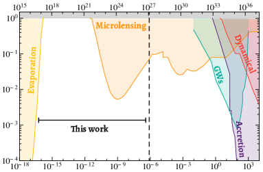
Because we are focusing in physics beyond the SM, the PT will take place at a temperature higher than that of the EW scale (around TeV). We will see that the corresponding enhancement appears in the range from to . Note that this includes the so-called asteroid mass range, where no stringent bounds have been found so far [42, 43], see Fig. 1.
The model. The properties of our strongly coupled, beyond the SM fluid will be investigated using the gauge/gravity duality or, in short, holography [44]. This correspondence provides a link between states of strongly coupled gauge theories and solutions to classical gravity in one extra dimension. Let us now discuss what these solutions in the gravity side of the duality and the corresponding features of the dual field theory are.
We consider a five-dimensional Einstein-scalar model described by the action
| (1) |
Here is the five-dimensional Ricci scalar, is the determinant of the space-time metric , and is the five-dimensional Newton constant. Note we are working in natural units, . Holography relates the scalar field to the gauge coupling of the dual field theory. The fall-off of the scalar near the boundary induces an explicit breaking of conformal invariance. This introduces an energy scale, , which is related to the critical temperature of the theory.
For simplicity, we assume that the potential comes from a superpotential via the usual relation
| (2) |
We stress that this choice has nothing to do with supersymmetry. Rather, we choose this particular potential so that the model coincides with that of [38, 39, 40, 41], in which the choice is made for convenience. The superpotential reads
| (3) |

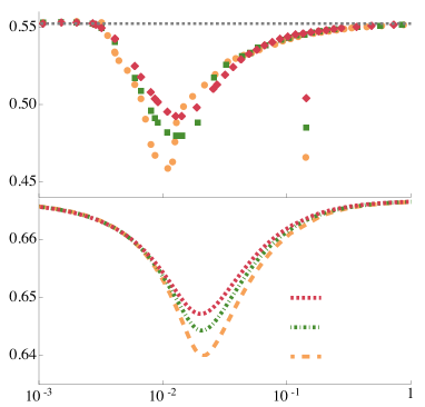
The reason why this model has caught so much attention is because by changing the parameters and one can easily obtain a first-order PT [45]. For definiteness, we will fix and let vary. Remarkably, the order of the PT changes when is tuned: below a certain value the theory undergoes a first-order PT. When , a critical point where a second-order PT takes place is found. Finally, if there is a SC between the two phases. This is the case we focus on. Numerically, we can determine that .
We are interested in black brane solutions of (1) that asymptote to Anti-de Sitter (AdS) space at infinity. We construct them following standard techniques 111See [97] for instance. Alternatively, a shooting method could be used [98], which has the advantage that the energy density and pressure can be computed from the fall off of the energy momentum tensor using holographic renormalization [99]. The latter method gives better control over the numerics. The properties of these black branes give us the features of the dual plasma. For instance, the temperature and entropy density of the states of the plasma are read off from the surface gravity and area density of these black brane solutions, respectively. Next, the pressure can be obtained by integrating the entropy density,
| (4) |
Finally, the energy density follows from the first law . With this information we can construct the two quantities needed to simulate PBH formation, namely the speed of sound squared and the ratio between the pressure and the energy density,
| (5) |
Both are shown in Fig. 2 for different choices of . Note that the critical temperature is defined as the temperature for which reaches the minimum.
Primordial Black Hole Formation. So far, we have examined the properties of a strongly coupled fluid, which models a candidate for a completion of the SM. As we have seen, the thermodynamic properties of this fluid depend on a parameter that we can adjust, and whose value affects the nature of the PT in its EoS.
The situation that we have in mind is that a such fluid fills the Universe at some point during its cosmological evolution. At this stage, the Universe is approximately homogeneous, isotropic and expanding. Thus, it is well described by a Friedmann–Lemaître–Robertson–Walker (FLRW) metric. On top of this background, we find curvature perturbations, seeded, for example, by quantum fluctuations during Inflation. We want to examine when such perturbations collapse into black holes.
For that we will need to solve Einstein’s equations,
| (6) |
where is the Ricci tensor in four dimensions, stands for its trace, is the spacetime metric, is the four-dimensional Newton’s constant and is the energy-momentum of the fluid. We assume that dissipative effects are not important, meaning that the energy-momentum tensor takes the form of a perfect fluid
| (7) |
with the fluid velocity. It is thus given in terms of the energy density and pressure, computed earlier. Moreover, we assume spherical symmetry, which we incorporate into our ansatz for the metric
| (8) |
Here, is the metric of a two-sphere with unit radius. Also, we will refer to as the cosmic time, as the lapse function, and as the areal radius. From the latter we can define the Misner–Sharp mass as the mass inside the surface given by constant,
| (9) |
With this particular ansatz, the system of Eqs. (6) can be expressed in the form worked out by Misner and Sharp [47] in the comoving gauge. For nonconstant EoS like ours, they take the form written in [32], in which the appropriate initial conditions are also discussed. Like there, we solve them numerically using pseudospectral methods (see also [48]).
As we anticipated, in our simulations, the Universe is initially described by a very small, superhorizon scale perturbation on top of our fluid at some constant density. If there were no perturbations, the Universe would remain homogeneous and isotropic. We can think of this as the background solution to Eqs. (6). In this case, it is customary to use Eq. (9) to define the corresponding horizon mass,
| (10) |
where we have used that is the Hubble radius and depends only on time, with the subindex standing for “background.” It is useful to keep in mind that when it comes to expressing our results in solar masses.
On top of this homogeneous Universe, we consider a cosmological perturbation that reenters the horizon at (an expression for will be given later). As we will see, there will be an enhancement in the PBH production for perturbations reentering when the SC is taking place. The mass of the statistically significant black holes formed is expected to be comparable to , the horizon mass evaluated at [49, 50]. For that reason we can use Eq. (10) to estimate the peak in the mass distribution of PBHs. Note that scales with (and is in our model when the transition occurs 222Note that this means we are fixing , with the radius of the asymptotic AdS space.). This means that scales as . Setting TeV we would get a peak around , above the constraint coming from Hawking evaporation. Furthermore, we require that is above the temperature of the electroweak PT (TeV), below which we trust CDM-SM. This implies that the position of the peak will be below . Thus, our model produces PBHs in the range of roughly for TeV.
The fluctuations we consider are adiabatic, and will therefore be frozen at superhorizon scales (). Consequently, at these scales the spacetime metric can be modeled by a FLRW metric with a non-constant curvature [52, 53, 54].
| (11) |
This serves to establish the initial conditions to evolve Eqs. (6). Note that connects to the hydrodynamic variable of the cosmological fluctuation at superhorizon scales [53, 54], which is useful to set up the initial conditions for the numerical simulation [32]. Given , the corresponding superhorizon scales, radiation-dominated compaction is written as . It represents twice the mass excess with respect to the background solution within the volume of radius . This function generically possesses a maximum at a certain , which, in turn, sets the amplitude of the cosmological fluctuation, [52, 54, 55]. It also allows us to define the time of horizon crossing as . Gravitational collapse into a black hole will occur for amplitudes above a certain threshold value , which we discuss next.
Threshold values. Following [32], we compute numerically the thresholds of PBH formation for the holographic EoS constructed in Eq. (5). Since for our simulations we will take a nearly flat scale-invariant power spectrum (PS) with , our perturbations can be appropriately modeled by a polynomial profile [56] with an index [57, 58]. The results corresponding to this choice are shown in Fig. 3. As expected, when approaches the critical value, the decrease in and significant decrease in trigger a reduction of the threshold. Remarkably, the diminution in threshold values is much more significant than during the QCD crossover. When taking the same curvature profile in the latter case, the relative deviation of the threshold with respect to the radiation-dominated era is found to be [32] at the peak value. In the present scenario, we encounter sizable reductions near the critical point, of around , and for and respectively.
PBHs mass function. Let us now turn to analyze the phenomenological implications of our smooth beyond the SM PT concerning the distribution of PBHs masses. We start by assuming that sufficiently large primordial density fluctuations leading to PBH formation are Gaussian distributed [59], with variance and probability density function .
To obtain concrete quantitative results we are forced to make a choice for the PS. This will be our main assumption, and the final distribution of PBHs masses will depend on this choice strongly. For instance, if we chose a monochromatic PS, the effect of the presence of the crossover would be very mild. In contrast, there are generic qualitative effects present as long as the PS is sufficiently broad and probes all the relevant scales. For concreteness, we consider a nearly flat, scale-invariant PS with shape . This is a common choice [60, 61, 62, 63]. The amplitude is related to the fraction of PBHs that constitute the DM. Additionally, is the spectral index at PBH scales, which we take in the range . We stress that our results are also sensitive to this choice but that there are notable generic features that extend for a wider range of . We will comment on this later. Furthermore, and are chosen so that the range of masses is accessed by the PS. Such a PS is realized in some inflationary models with convenient engineering of the inflationary PS [64, 65, 66, 67, 68].
We write the standard deviation of the density perturbations as , where is a function related to the energy dependence of the EoS 333see Eq. (2.22) in [32] and is shown in Fig. 4 (bottom). In fact, this gives a good approximation to the actual value of .
Knowing the PS, the relative abundance of PBHs can be computed. For that we will make two approximations. First, we take the mass of the PBH that forms from the collapse of a particular curvature perturbation to be proportional to the horizon mass (10) at its time of horizon crossing, . This is also a common assumption [70]. While facilitating computations, it neglects effects near the critical PBH mass regime [71, 72]. However, these effects are subdominant with respect to the decrease in the threshold value when it comes to estimate PBH abundances. Accounting for these effects, such as a shift in the peak and a change on the shape around the peak of the mass function, is beyond the scope of the present work. Second, we use the Press-Schechter formalism [73]. Then the mass function, defined so that is the fraction of PBHs between and [74, 30], reads
| (12) |
where and the PBH mass abundance is
| (13) |
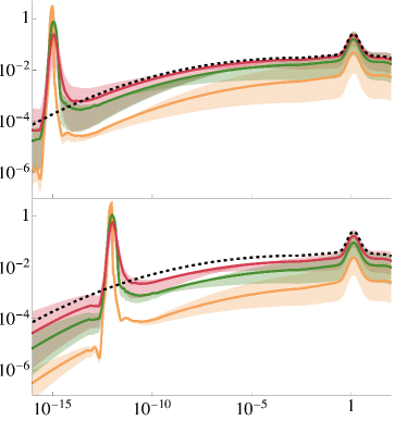
In Eq. (12), corresponds to the horizon mass at the time of matter-radiation equality [75]. The total abundance of PBHs in the form of DM is then . Using the numerical results of the threshold presented in Fig. 3 (top), we compute the mass function of PBH formation following Eqs. (12) and (13). If all the DM consists of PBHs, , we get in this scenario that . Therefore, despite the remarkable reduction in the threshold values, we still need a significant enhancement of the amplitude of the PS on the PBH scales (like when only the QCD crossover is considered [30]).
In Fig.4, we show the mass function obtained from the holographic model with TeV (top) and TeV (bottom), together with the QCD crossover. The peak originated during the strongly coupled crossover is patent. As approaches the enhancement strengthens and the peak sharpens. This enhancement causes the rest of the mass function to drop (so that in all cases). We have checked that these are generic features for a range of wider than just 444Note this is a similar range to the one used in [60]., the main difference being the enhanced production of heavy (light) PBHs when is sensitively smaller than (closer to) . Actually, it is already clear from Fig. 4 that a mild modification of the spectral index significantly modifies the abundance in the region of the peak at the stellar mass range, corresponding to the QCD crossover.
Discussion. In this Letter, we have studied for the first time implications of the presence of a strongly coupled SC in the very early Universe regarding PBH formation. We saw that it can have a significant impact due to the reduction in the EoS and sound speed of the cosmological fluid, more pronounced the closer the theory flows near the critical point.
A two-peak mass function is obtained as a result with the choice of a particular broad PS. The peaks correspond to the beyond the SM and QCD crossovers. It has been observed that the QCD peak alone seems unable to account for all the DM when inferred merging rates from GW observations are considered [32, 31, 77]. This is not the case in our model, since the presence of our strongly coupled crossover and consequent peak at the asteroid mass range lower the amount of PBHs needed in the solar mass range. Despite its simplicity, the model is flexible enough so that an appropriate choice of and may match those inferred merging rates. Better statistical estimation of the PBH abundances would be needed to find accurate results though [78, 59], as well as better exploration of the critical PBH mass regime.
Our work can be extended in many different directions. First, it is natural to ask what happens when the PT becomes of the first order. There have been already some approaches to this problem [79, 80, 81, 82]. It has an additional complication since, as we mentioned at the beginning, bubbles are expected to nucleate in such scenario. Then PBHs are obtained not only by the collapse of primordial perturbations, but also in the shrinking of false vacuum bubbles in the final stage of the process [83, 84, 85, 86]. An appropriate approach could be that of [87], in which holography is used to evolve the stress tensor of the microscopic quantum theory and seed Einstein’s equations with its expectation value. Then, the dynamical evolution of the bubble can be performed, without any hydrodynamical approximation, and the interplay between bubble nucleation and PBH formation can be examined.
On the other hand, our results should not depend much on the fact that the theory beyond the SM undergoing a SC is strongly coupled, since the information read off from the holographic model (1) is just the EoS and the speed of sound; see Eq. (5). Thus, it would be interesting to perform similar investigations in weakly coupled models, where we expect to find akin phenomenology. In fact, one could just demand thermodynamic consistency and causality and perform an alike study several EoSs featuring a SC with similar to the ones we discussed 555We thank the anonymous referee for pointing this possible approach out..
Additionally, it is well known that the spin of the PBHs formed during a radiation-dominated era is small [89] but may be larger for softer EoSs [90, 91]. Consequently, the sharp reduction of could significantly affect the spin of the PBHs at the corresponding scales. At the same time, stochastic GW background induced by scalar perturbations is also sensitive to , so it would be desirable to check if for the cases discussed here it lies in the range of LISA frequencies [92, 93, 94, 95] and constitute an evidence of the presence of such a SC [96].
In summary, we have shown how our SC at energies above the EW scale has significant phenomenological impact. We hope our observations serve as the starting point for exciting future investigations considering PBHs as probes for beyond the SM physics.
Acknowledgements.
Acknowledgments We thank Jaume Garriga, Cristiano Germani, David Mateos, Marc Oncins, Mikel Sanchez–Garitaonandia, Yuichiro Tada and Chulmoon Yoo for useful discussions and comments. Nordita is supported in part by NordForsk. A.E acknowledges support from the JSPS Postdoctoral Fellowships for Research in Japan (Graduate School of Sciences, Nagoya University).References
- Abbott et al. [2016] B. P. Abbott et al. (LIGO Scientific, Virgo), Phys. Rev. Lett. 116, 061102 (2016), arXiv:1602.03837 [gr-qc] .
- Hindmarsh et al. [2021] M. B. Hindmarsh, M. Lüben, J. Lumma, and M. Pauly, SciPost Phys. Lect. Notes 24, 1 (2021), arXiv:2008.09136 [astro-ph.CO] .
- Guo et al. [2021] H.-K. Guo, K. Sinha, D. Vagie, and G. White, JCAP 01, 001 (2021), arXiv:2007.08537 [hep-ph] .
- Kalogera et al. [2021] V. Kalogera et al., (2021), arXiv:2111.06990 [gr-qc] .
- Caprini et al. [2020] C. Caprini et al., JCAP 03, 024 (2020), arXiv:1910.13125 [astro-ph.CO] .
- Aoki et al. [2006] Y. Aoki, G. Endrodi, Z. Fodor, S. D. Katz, and K. K. Szabo, Nature 443, 675 (2006), arXiv:hep-lat/0611014 [hep-lat] .
- Kajantie et al. [1996] K. Kajantie, M. Laine, K. Rummukainen, and M. E. Shaposhnikov, Phys. Rev. Lett. 77, 2887 (1996), arXiv:hep-ph/9605288 .
- Laine and Rummukainen [1998a] M. Laine and K. Rummukainen, Phys. Rev. Lett. 80, 5259 (1998a), arXiv:hep-ph/9804255 .
- Rummukainen et al. [1998] K. Rummukainen, M. Tsypin, K. Kajantie, M. Laine, and M. E. Shaposhnikov, Nucl. Phys. B 532, 283 (1998), arXiv:hep-lat/9805013 .
- Carena et al. [1996] M. Carena, M. Quiros, and C. E. M. Wagner, Phys. Lett. B 380, 81 (1996), arXiv:hep-ph/9603420 .
- Delepine et al. [1996] D. Delepine, J. M. Gerard, R. Gonzalez Felipe, and J. Weyers, Phys. Lett. B 386, 183 (1996), arXiv:hep-ph/9604440 .
- Laine and Rummukainen [1998b] M. Laine and K. Rummukainen, Nucl. Phys. B 535, 423 (1998b), arXiv:hep-lat/9804019 .
- Huber and Schmidt [2001] S. J. Huber and M. G. Schmidt, Nucl. Phys. B 606, 183 (2001), arXiv:hep-ph/0003122 .
- Grojean et al. [2005] C. Grojean, G. Servant, and J. D. Wells, Phys. Rev. D 71, 036001 (2005), arXiv:hep-ph/0407019 .
- Huber et al. [2007] S. J. Huber, T. Konstandin, T. Prokopec, and M. G. Schmidt, Nucl. Phys. A 785, 206 (2007), arXiv:hep-ph/0608017 .
- Profumo et al. [2007] S. Profumo, M. J. Ramsey-Musolf, and G. Shaughnessy, JHEP 08, 010 (2007), arXiv:0705.2425 [hep-ph] .
- Barger et al. [2008] V. Barger, P. Langacker, M. McCaskey, M. J. Ramsey-Musolf, and G. Shaughnessy, Phys. Rev. D 77, 035005 (2008), arXiv:0706.4311 [hep-ph] .
- Laine et al. [2013] M. Laine, G. Nardini, and K. Rummukainen, JCAP 01, 011 (2013), arXiv:1211.7344 [hep-ph] .
- Dorsch et al. [2013] G. C. Dorsch, S. J. Huber, and J. M. No, JHEP 10, 029 (2013), arXiv:1305.6610 [hep-ph] .
- Damgaard et al. [2016] P. H. Damgaard, A. Haarr, D. O’Connell, and A. Tranberg, JHEP 02, 107 (2016), arXiv:1512.01963 [hep-ph] .
- Georgi and Glashow [1974] H. Georgi and S. L. Glashow, Phys. Rev. Lett. 32, 438 (1974).
- Pati and Salam [1974] J. C. Pati and A. Salam, Phys. Rev. D 10, 275 (1974), [Erratum: Phys.Rev.D 11, 703–703 (1975)].
- Zel’dovich and Novikov [1967] Y. B. Zel’dovich and I. D. Novikov, sovast 10, 602 (1967).
- Hawking [1971] S. Hawking, Mon. Not. Roy. Astron. Soc. 152, 75 (1971).
- Carr and Hawking [1974] B. J. Carr and S. W. Hawking, Monthly Notices of the Royal Astronomical Society 168, 399 (1974).
- Escrivà et al. [2022a] A. Escrivà, F. Kuhnel, and Y. Tada, (2022a), arXiv:2211.05767 [astro-ph.CO] .
- Chapline [1975] G. F. Chapline, Nature 253, 251 (1975).
- Carr [1975] B. J. Carr, Astrophys. J. 201, 1 (1975).
- Jedamzik [1997] K. Jedamzik, Phys. Rev. D 55, 5871 (1997), arXiv:astro-ph/9605152 .
- Byrnes et al. [2018] C. T. Byrnes, M. Hindmarsh, S. Young, and M. R. S. Hawkins, JCAP 08, 041 (2018), arXiv:1801.06138 [astro-ph.CO] .
- Franciolini et al. [2022] G. Franciolini, I. Musco, P. Pani, and A. Urbano, (2022), arXiv:2209.05959 [astro-ph.CO] .
- Escrivà et al. [2022b] A. Escrivà, E. Bagui, and S. Clesse, arXiv e-prints , arXiv:2209.06196 (2022b), arXiv:2209.06196 [astro-ph.CO] .
- Carr et al. [2021a] B. Carr, K. Kohri, Y. Sendouda, and J. Yokoyama, Rept. Prog. Phys. 84, 116902 (2021a), arXiv:2002.12778 [astro-ph.CO] .
- Green and Kavanagh [2021] A. M. Green and B. J. Kavanagh, Journal of Physics G Nuclear Physics 48, 043001 (2021), arXiv:2007.10722 [astro-ph.CO] .
- Kavanagh [2019] B. J. Kavanagh, “bradkav/pbhbounds: Release version,” (2019).
- Kribs and Neil [2016] G. D. Kribs and E. T. Neil, Int. J. Mod. Phys. A 31, 1643004 (2016), arXiv:1604.04627 [hep-ph] .
- Tulin and Yu [2018] S. Tulin and H.-B. Yu, Phys. Rept. 730, 1 (2018), arXiv:1705.02358 [hep-ph] .
- Bea et al. [2021a] Y. Bea, J. Casalderrey-Solana, T. Giannakopoulos, D. Mateos, M. Sanchez-Garitaonandia, and M. Zilhão, Phys. Rev. D 104, L121903 (2021a), arXiv:2104.05708 [hep-th] .
- Bea et al. [2022] Y. Bea, J. Casalderrey-Solana, T. Giannakopoulos, A. Jansen, D. Mateos, M. Sanchez-Garitaonandia, and M. Zilhão, (2022), arXiv:2202.10503 [hep-th] .
- Ares et al. [2020] F. R. Ares, M. Hindmarsh, C. Hoyos, and N. Jokela, JHEP 21, 100 (2020), arXiv:2011.12878 [hep-th] .
- Bea et al. [2021b] Y. Bea, J. Casalderrey-Solana, T. Giannakopoulos, A. Jansen, S. Krippendorf, D. Mateos, M. Sanchez-Garitaonandia, and M. Zilhão, (2021b), arXiv:2112.15478 [hep-th] .
- Katz et al. [2018] A. Katz, J. Kopp, S. Sibiryakov, and W. Xue, JCAP 12, 005 (2018), arXiv:1807.11495 [astro-ph.CO] .
- Montero-Camacho et al. [2019] P. Montero-Camacho, X. Fang, G. Vasquez, M. Silva, and C. M. Hirata, JCAP 08, 031 (2019), arXiv:1906.05950 [astro-ph.CO] .
- Maldacena [1998] J. M. Maldacena, Adv. Theor. Math. Phys. 2, 231 (1998), arXiv:hep-th/9711200 .
- Bea and Mateos [2018] Y. Bea and D. Mateos, JHEP 08, 034 (2018), arXiv:1805.01806 [hep-th] .
- Note [1] See [97] for instance. Alternatively, a shooting method could be used [98], which has the advantage that the energy density and pressure can be computed from the fall off of the energy momentum tensor using holographic renormalization [99]. The latter method gives better control over the numerics.
- Misner and Sharp [1964] C. W. Misner and D. H. Sharp, Phys. Rev. 136, B571 (1964).
- Escrivà [2020] A. Escrivà, Phys. Dark Univ. 27, 100466 (2020), arXiv:1907.13065 [gr-qc] .
- Carr [1977] B. J. Carr, Astronomy and Astrophysics 56, 377 (1977).
- Germani and Musco [2019] C. Germani and I. Musco, Phys. Rev. Lett. 122, 141302 (2019), arXiv:1805.04087 [astro-ph.CO] .
- Note [2] Note that this means we are fixing , with the radius of the asymptotic AdS space.
- Shibata and Sasaki [1999] M. Shibata and M. Sasaki, Phys. Rev. D 60, 084002 (1999), arXiv:gr-qc/9905064 [gr-qc] .
- Polnarev and Musco [2007] A. G. Polnarev and I. Musco, Classical and Quantum Gravity 24, 1405 (2007), arXiv:gr-qc/0605122 [gr-qc] .
- Harada et al. [2015] T. Harada, C.-M. Yoo, T. Nakama, and Y. Koga, Phys. Rev. D 91, 084057 (2015), arXiv:1503.03934 [gr-qc] .
- Musco [2019] I. Musco, Phys. Rev. D 100, 123524 (2019), arXiv:1809.02127 [gr-qc] .
- Escrivà et al. [2021] A. Escrivà, C. Germani, and R. K. Sheth, JCAP 01, 030 (2021), arXiv:2007.05564 [gr-qc] .
- Escrivà et al. [2020] A. Escrivà, C. Germani, and R. K. Sheth, Phys. Rev. D 101, 044022 (2020), arXiv:1907.13311 [gr-qc] .
- Musco et al. [2021] I. Musco, V. De Luca, G. Franciolini, and A. Riotto, Phys. Rev. D 103, 063538 (2021), arXiv:2011.03014 [astro-ph.CO] .
- Yoo et al. [2021] C.-M. Yoo, T. Harada, S. Hirano, and K. Kohri, PTEP 2021, 013E02 (2021), arXiv:2008.02425 [astro-ph.CO] .
- Carr et al. [2021b] B. Carr, S. Clesse, J. García-Bellido, and F. Kühnel, Phys. Dark Univ. 31, arXiv:1906.08217 (2021b), arXiv:1906.08217 [astro-ph.CO] .
- De Luca et al. [2020] V. De Luca, G. Franciolini, and A. Riotto, Phys. Lett. B 807, 135550 (2020), arXiv:2001.04371 [astro-ph.CO] .
- De Luca et al. [2021] V. De Luca, G. Franciolini, and A. Riotto, Phys. Rev. Lett. 126, 041303 (2021), arXiv:2009.08268 [astro-ph.CO] .
- Sugiyama et al. [2021] S. Sugiyama, V. Takhistov, E. Vitagliano, A. Kusenko, M. Sasaki, and M. Takada, Phys. Lett. B 814, 136097 (2021), arXiv:2010.02189 [astro-ph.CO] .
- Wands [1999] D. Wands, Phys. Rev. D 60, 023507 (1999), arXiv:gr-qc/9809062 .
- Leach and Liddle [2001] S. M. Leach and A. R. Liddle, Phys. Rev. D 63, 043508 (2001), arXiv:astro-ph/0010082 .
- Leach et al. [2001] S. M. Leach, M. Sasaki, D. Wands, and A. R. Liddle, Phys. Rev. D 64, 023512 (2001), arXiv:astro-ph/0101406 .
- Byrnes et al. [2019] C. T. Byrnes, P. S. Cole, and S. P. Patil, JCAP 06, 028 (2019), arXiv:1811.11158 [astro-ph.CO] .
- Franciolini and Urbano [2022] G. Franciolini and A. Urbano, (2022), arXiv:2207.10056 [astro-ph.CO] .
- Note [3] See Eq. (2.22) in [32].
- Carr and Kuhnel [2022] B. Carr and F. Kuhnel, SciPost Phys. Lect. Notes 48, 1 (2022), arXiv:2110.02821 [astro-ph.CO] .
- Niemeyer and Jedamzik [1998] J. C. Niemeyer and K. Jedamzik, Phys. Rev. Lett. 80, 5481 (1998), arXiv:astro-ph/9709072 [astro-ph] .
- Musco and Miller [2013] I. Musco and J. C. Miller, Classical and Quantum Gravity 30, 145009 (2013), arXiv:1201.2379 [gr-qc] .
- Press and Schechter [1974] W. H. Press and P. Schechter, Astrophys. J. 187, 425 (1974).
- Sasaki et al. [2018] M. Sasaki, T. Suyama, T. Tanaka, and S. Yokoyama, Classical and Quantum Gravity 35, 063001 (2018), arXiv:1801.05235 [astro-ph.CO] .
- Nakama et al. [2017] T. Nakama, J. Silk, and M. Kamionkowski, Phys. Rev. D 95, 043511 (2017), arXiv:1612.06264 [astro-ph.CO] .
- Note [4] Note this is a similar range to the one used in [60].
- Juan et al. [2022] J. I. Juan, P. D. Serpico, and G. Franco Abellán, JCAP 07, 009 (2022), arXiv:2204.07027 [astro-ph.CO] .
- Germani and Sheth [2020] C. Germani and R. K. Sheth, Phys. Rev. D 101, 063520 (2020), arXiv:1912.07072 [astro-ph.CO] .
- Jedamzik and Niemeyer [1999] K. Jedamzik and J. C. Niemeyer, Phys. Rev. D 59, 124014 (1999), arXiv:astro-ph/9901293 .
- Liu et al. [2022] J. Liu, L. Bian, R.-G. Cai, Z.-K. Guo, and S.-J. Wang, Phys. Rev. D 105, L021303 (2022), arXiv:2106.05637 [astro-ph.CO] .
- Davoudiasl [2019] H. Davoudiasl, Phys. Rev. Lett. 123, 101102 (2019), arXiv:1902.07805 [hep-ph] .
- He et al. [2022] S. He, L. Li, Z. Li, and S.-J. Wang, (2022), arXiv:2210.14094 [hep-ph] .
- Baker et al. [2021a] M. J. Baker, M. Breitbach, J. Kopp, and L. Mittnacht, (2021a), arXiv:2105.07481 [astro-ph.CO] .
- Baker et al. [2021b] M. J. Baker, M. Breitbach, J. Kopp, and L. Mittnacht, (2021b), arXiv:2110.00005 [astro-ph.CO] .
- Gross et al. [2021] C. Gross, G. Landini, A. Strumia, and D. Teresi, JHEP 09, 033 (2021), arXiv:2105.02840 [hep-ph] .
- Kawana and Xie [2022] K. Kawana and K.-P. Xie, Phys. Lett. B 824, 136791 (2022), arXiv:2106.00111 [astro-ph.CO] .
- Ecker et al. [2022] C. Ecker, W. van der Schee, D. Mateos, and J. Casalderrey-Solana, JHEP 03, 137 (2022), arXiv:2109.10355 [hep-th] .
- Note [5] We thank the anonymous referee for pointing this possible approach out.
- Harada et al. [2021] T. Harada, C.-M. Yoo, K. Kohri, Y. Koga, and T. Monobe, Astrophys. J. 908, 140 (2021), arXiv:2011.00710 [astro-ph.CO] .
- Harada et al. [2017] T. Harada, C.-M. Yoo, K. Kohri, and K.-I. Nakao, Phys. Rev. D 96, 083517 (2017), [Erratum: Phys.Rev.D 99, 069904 (2019)], arXiv:1707.03595 [gr-qc] .
- Kokubu et al. [2018] T. Kokubu, K. Kyutoku, K. Kohri, and T. Harada, Phys. Rev. D 98, 123024 (2018), arXiv:1810.03490 [astro-ph.CO] .
- Bartolo et al. [2019] N. Bartolo, V. De Luca, G. Franciolini, A. Lewis, M. Peloso, and A. Riotto, Phys. Rev. Lett. 122, 211301 (2019), arXiv:1810.12218 [astro-ph.CO] .
- Oncins [2022] M. Oncins, (2022), arXiv:2205.14722 [astro-ph.CO] .
- Barausse et al. [2020] E. Barausse et al., Gen. Rel. Grav. 52, 81 (2020), arXiv:2001.09793 [gr-qc] .
- Cai et al. [2019] R.-g. Cai, S. Pi, and M. Sasaki, Phys. Rev. Lett. 122, 201101 (2019), arXiv:1810.11000 [astro-ph.CO] .
- Abe et al. [2021] K. T. Abe, Y. Tada, and I. Ueda, JCAP 06, 048 (2021), arXiv:2010.06193 [astro-ph.CO] .
- Gubser and Nellore [2008] S. S. Gubser and A. Nellore, Phys. Rev. D 78, 086007 (2008), arXiv:0804.0434 [hep-th] .
- Dias et al. [2016] O. J. C. Dias, J. E. Santos, and B. Way, Class. Quant. Grav. 33, 133001 (2016), arXiv:1510.02804 [hep-th] .
- de Haro et al. [2001] S. de Haro, S. N. Solodukhin, and K. Skenderis, Commun. Math. Phys. 217, 595 (2001), arXiv:hep-th/0002230 .