SuperFusion: Multilevel LiDAR-Camera Fusion
for Long-Range HD Map Generation

Abstract

High-definition (HD) semantic map generation of the environment is an essential component of autonomous driving. Existing methods have achieved good performance in this task by fusing different sensor modalities, such as LiDAR and camera. However, current works are based on raw data or network feature-level fusion and only consider short-range HD map generation, limiting their deployment to realistic autonomous driving applications. In this paper, we focus on the task of building the HD maps in both short ranges, i.e., within 30 m, and also predicting long-range HD maps up to 90 m, which is required by downstream path planning and control tasks to improve the smoothness and safety of autonomous driving. To this end, we propose a novel network named SuperFusion, exploiting the fusion of LiDAR and camera data at multiple levels. We use LiDAR depth to improve image depth estimation and use image features to guide long-range LiDAR feature prediction. We benchmark our SuperFusion on the nuScenes dataset and a self-recorded dataset and show that it outperforms the state-of-the-art baseline methods with large margins on all intervals. Additionally, we apply the generated HD map to a downstream path planning task, demonstrating that the long-range HD maps predicted by our method can lead to better path planning for autonomous vehicles. Our code and self-recorded dataset will be available at https://github.com/haomo-ai/SuperFusion.

1 Introduction

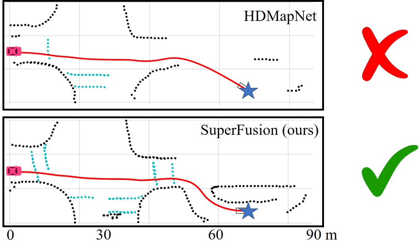
Figure 1: Long-range HD map generation for path planning. The red car represents the current position of the car, and the blue star is the goal. The upper figure shows that the baseline method only generates short-range HD maps, leading to lousy planning results. The lower one shows that our SuperFusion generates accurate HD maps in both short and long ranges, which serves online path planning well for autonomous driving.

Detecting street lanes and generating semantic high-definition (HD) maps are essential for autonomous vehicles to achieve self-driving. The HD map consists of semantic layers with lane boundaries, road dividers, pedestrian crossings, etc., which provide precise location information about nearby infrastructure, roads, and environments to navigate autonomous vehicles safely [14].

The traditional way builds the HD maps offline by firstly recording point clouds, then creating globally consistent maps using SLAM [41], and finally manually annotating semantics in the maps. Although some autonomous driving companies have created accurate HD maps following such a paradigm, it requires too much human effort and needs continuous updating. Since autonomous vehicles are typically equipped with various sensors, exploiting the onboard sensor data to build local HD maps for online applications attracts much attention. Existing methods usually extract lanes and crossings on the bird’s-eye view (BEV) representation of either camera data [43] or LiDAR data [22]. Recently, several methods [22, 26, 32] show advances in fusing multi-sensor modalities. They leverage the complementary information from both sensors to improve the HD map generation performance. Albeit improvements, existing methods fuse LiDAR and camera data in simple ways, either on the raw data level [38, 37], feature level [2, 51], or final BEV level [22, 26, 32], which do not fully exploit the advantages from both modalities. Besides, existing methods only focus on short-range HD map generation due to the limited sensor measurement range, i.e., within 30 m, which limits their usage in downstream applications such as path planning and motion control in real autonomous driving scenarios. As shown in Fig. 1, when the generated HD map is too short, the planning method may create a non-smooth path that requires frequent replanning due to limited perception distances, or even a path that intersects with the sidewalk. This can lead to frustration for users, as rapidly changing controls can degrade their comfort level.

To tackle the problem mentioned above, in this paper, we propose a multilevel LiDAR-camera fusion method, dubbed SuperFusion. It fuses the LiDAR and camera data at three different levels. In the data-level fusion, it combines the projected LiDAR data with images as the input of the camera encoder and uses LiDAR depth to supervise the camera-to-BEV transformation. The feature-level fusion uses camera features to guide the LiDAR features on long-range LiDAR BEV feature prediction using a cross-attention mechanism. In the final BEV-level fusion, our method exploits a BEV alignment module to align and fuse camera and LiDAR BEV features. Using our proposed multilevel fusion strategy, SuperFusion generates accurate HD maps in the short range and also predicts accurate semantics in the long-range distances, where the raw LiDAR data may not capture. We thoroughly evaluate our SuperFusion and compare it with the state-of-the-art methods on the publically available nuScenes dataset and our own dataset recorded in real-world self-driving scenarios. The experimental results consistently show that our method outperforms the baseline methods significantly by a large margin on all intervals. Furthermore, we provide the application results of using our generated HD maps for path planning, showing the superiority of our proposed fusion method for long-range HD map generation.

Our contributions can be summarized as: i) our proposed novel multilevel LiDAR-camera fusion network fully leverages the information from both modalities and generates high-quality fused BEV features to support different tasks; ii) our SuperFusion surpasses the state-of-the-art fusion methods in both short-range and long-range HD map generation by a large margin; iii) to the best of our knowledge, our work is the first to achieve long-range HD map generation, i.e., up to 90 m, benefiting the autonomous driving downstream planning task; iv) we release our code as well as a new dataset for evaluating long-range HD map generation tasks.

2 Related Work

BEV Representation. The bird’s-eye view (BEV) perception has attracted enormous attention from industry and academia [39]. BEV representations are easy to be deployed in various autonomous driving downstream tasks such as object detection and tracking [54], motion planning [52], traffic participant behavior prediction [18], etc. Most recently, multiple works have used BEV representation for sensor fusion and achieved performance improvement in tasks like lane detection [26, 32] and occupancy prediction [16, 11]. It has become a new favorite as a straightforward and interpretable way to fuse data from multiple modalities, including cameras [43], LiDARs [22], and radars [8]. For LiDAR and radar data, the 3D information is naturally available and thus can be used to generate BEV views easily by an XY-plane projection [36, 3]. To avoid information loss along the Z-axis, modern methods generate BEV features via point cloud encoders, such as PointPillars [21] and VoxelNet [53].

Camera-to-BEV Transformation. The depth information is lost for images captured in perspective view (PV). Therefore, the transformation from PV to BEV is an ill-posed problem and remains unsolved. Inverse perspective mapping (IPM) [40] is the first work tackling this problem under a flat-ground assumption. However, real autonomous driving scenarios are usually complex, and the flat-ground assumption is commonly violated. Many data-driven methods, including geometry-based and network-based transformation, have been proposed recently to make this PV-to-BEV transformation available in complex scenes [39]. The geometry-based methods achieve view transformation interpretably by using camera projection principles. Abbas et al. [1] estimate vanishing points and lines in the PV images to determine the homography matrix for IPM. Image depth estimation has also been applied to this task. For example, LSS [43] predicts a categorical depth distribution for each pixel and generates features for each pixel along the ray. After lifting the image into a frustum of features, it performs a sum pooling to splat frustum features into BEV features. Some works [34, 5, 48] also exploit semantic information to reduce the distortion caused by objects above the ground.

Existing network-based methods typically use multi-layer perceptrons (MLPs) and transformers [49] to model the view transformation. VED [35] utilizes a variational encoder-decoder with an MLP bottleneck layer to achieve PV-to-BEV transformation, while VPN [42] employs a two-layer MLP to map PV features to BEV features. Similarly, PON [46] uses a feature pyramid [29] to extract multi-resolution features and then collapses features along the height axis and expands along the depth axis using MLP to achieve view transformation. More recently, there are also works [25, 47, 55, 31] using transformers for PV-to-BEV transformation, which show accuracy improvements but are less efficient. Different from existing works, our method explores both sparse depth priors from LiDAR data and dense completed depth maps as supervision for more robust and reliable image depth prediction.

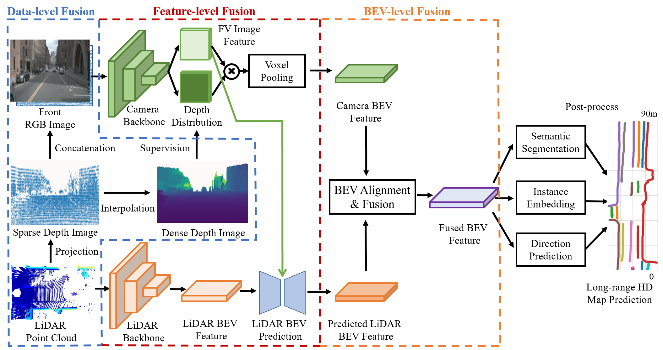
Figure 2: Pipeline overview of SuperFusion. Our method fuses camera and LiDAR data in three levels: the data-level fusion fuses depth information from LiDAR to improve the accuracy of image depth estimation, the feature-level fusion uses cross-attention for long-range LiDAR BEV feature prediction with the guidance of image features, and the BEV-level fusion aligns two branches to generate high-quality fused BEV features. Finally, the fused BEV features can support different heads, including semantic segmentation, instance embedding, and direction prediction, and finally post-processed to generate the HD map prediction.

LiDAR-Camera Fusion. The existing fusion strategies can be divided into three levels: data-level, feature-level, and BEV-level fusion. Data-level fusion methods [38, 37, 50, 24] project LiDAR point clouds to images using the camera projection matrix. The projected sparse depth map can be fed to the network with the image data [38, 37] or decorated with image semantic features [50, 24] to enhance the network inputs. Feature-level fusion methods [2, 51] incorporate different modalities in the feature space using transformers. They first generate LiDAR feature maps, then query image features on those LiDAR features using cross-attention, and finally concatenate them together for downstream tasks. BEV-level fusion methods [22, 26, 32] extract LiDAR and image BEV features separately and then fuse the BEV features by concatenation [22] or fusion modules [26, 32]. For example, HDMapNet [22] uses MLPs to map PV features to BEV features for the camera branch and uses PointPillars [21] to encode BEV features in the LiDAR branch. Recent BEVFusion works [26, 32] use LSS [43] for view transformation in the camera branch and VoxelNet [53] in the LiDAR branch and finally fuse them via a BEV alignment module. Unlike them, our method combines all three-level LiDAR and camera fusion to fully exploit the complementary attributes of these two sensor modalities.

HD Map Generation. The traditional way of reconstructing HD semantic maps is to aggregate LiDAR point clouds using SLAM algorithms [41] and then annotate manually, which is laborious and difficult to update. HDMapNet [22] is a pioneer work on local HD map construction without human annotations. It fuses LiDAR and six surrounding cameras in BEV space for semantic HD map generation. Besides that, VectorMapNet [30] represents map elements as a set of polylines and models these polylines with a set prediction framework, while Image2Map [47] utilizes a transformer to generate HD maps from images in an end-to-end fashion. Several works [13, 15, 7] also detect specific map elements such as lanes. However, previous works only segment maps in a short range, usually less than 30 m. Our method is the first work focusing on long-range HD map generation up to 90 m.

3 Methodology

This section presents the proposed SuperFusion for long-range HD map generation and prediction. The raw LiDAR and camera data have different characteristics. The LiDAR data provides accurate 3D structure information but suffers from disorderliness and sparseness. The camera data is compact, capturing more contextual information about the environment but missing depth information. As shown in Fig. 2, our method fuses camera and LiDAR data in three levels to compensate for the deficiencies and exploit advances of both modalities. In the data-level fusion (Sec. 3.1), we project LiDAR point clouds on image planes to get sparse depth images. We feed these sparse depth images together with RGB images as the input of the camera encoder and also use them to supervise the camera-to-BEV transformation module during training. In the feature-level fusion (Sec. 3.2), we leverage front-view camera features to guide the LiDAR BEV features on long-range predictions using a cross-attention interaction to achieve accurate long-range HD map prediction. In the final BEV-level fusion (Sec. 3.3), we design a BEV alignment module to align and fuse the camera and LiDAR BEV features. The fused BEV features can support different heads, including semantic segmentation, instance embedding, and direction prediction, and finally post-processed to generate the HD map prediction (Sec. 3.4).

3.1 Depth-Aware Camera-to-BEV Transformation

We first fuse the LiDAR and camera at the raw data level and leverage the depth information from LiDAR to help the camera lift features to BEV space. To this end, we propose a depth-aware camera-to-BEV transformation module, as shown in Fig. 2. It takes an RGB image $\mathbf{I}$ with the corresponding sparse depth image $\mathbf{{D}_{sparse}}$ as input. Such sparse depth image $\mathbf{{D}_{sparse}}$ is obtained by projecting the 3D LiDAR point cloud $\mathbf{P}$ to the image plane using the camera projection matrix. The camera backbone has two branches. The first branch extracts 2D image features $\mathbf{{F}}\in\mathbb{R}^{W_{F}\times H_{F}\times C_{F}}$, where $W_{F}$, $H_{F}$ and $C_{F}$ are the width, height and channel numbers. The second branch connects a depth prediction network, which estimates a categorical depth distribution $\mathbf{{D}}\in\mathbb{R}^{W_{F}\times H_{F}\times D}$ for each element in the 2D feature $\mathbf{{F}}$, where $D$ is the number of discretized depth bins. To better estimate the depth, we use a completion method [20] on $\mathbf{{D}_{sparse}}$ to generate a dense depth image $\mathbf{{D}_{dense}}$ and discretize the depth value of each pixel into depth bins, which is finally converted to a one-hot encoding vector to supervise the depth prediction network. The final frustum feature grid $\mathbf{M}$ is generated by the outer product of $\mathbf{{D}}$ and $\mathbf{{F}}$ as

$$\mathbf{M}(u,v)=\mathbf{D}(u,v)\otimes\mathbf{F}(u,v),$$ (1)

where $\mathbf{{M}}\in\mathbb{R}^{W_{F}\times H_{F}\times D\times C_{F}}$. Finally, each voxel in the frustum is assigned to the nearest pillar and a sum pooling is performed as in LSS [43] to create the camera BEV feature $\mathbf{{C}}~{}\in~{}\mathbb{R}^{W\times H\times C_{F}}$.

Our proposed depth-aware camera-to-BEV module differs from the existing depth prediction methods [43, 44]. The depth prediction in LSS [43] is only implicitly supervised by the semantic segmentation loss, which is not enough to generate accurate depth estimation. Different from that, we utilize the depth information from LiDAR as supervision. CaDDN [44] also uses LiDAR depth for supervision but without LiDAR as input, thus unable to generate a robust and reliable depth estimation. Our method uses both the completed dense LiDAR depth image for supervision and also the sparse depth image as an additional channel to the RGB image. In this way, our network exploits both a depth prior and an accurate depth supervision, thus generalizing well to different challenging environments.

3.2 Image-Guided LiDAR BEV Prediction

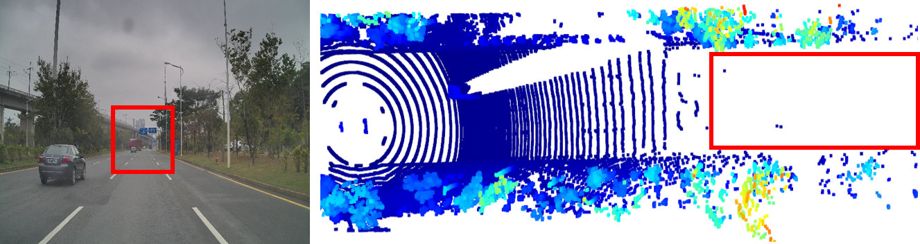
(a) The LiDAR usually has a short valid range for the ground plane, while the camera can see a much longer distance.

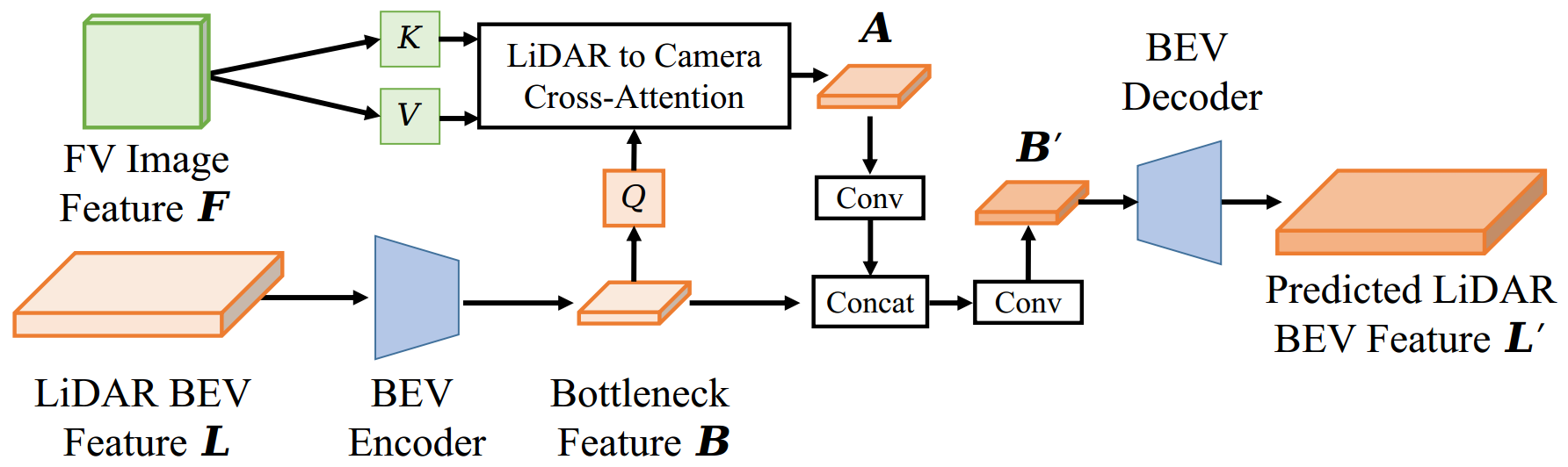
(b) LiDAR BEV prediction with cross-attention.

Figure 3: Image-guided LiDAR BEV Prediction.

In the LiDAR branch, we use PointPillars [21] plus dynamic voxelization [56] as the point cloud encoder to generate LiDAR BEV features $\mathbf{{L}}\in\mathbb{R}^{W\times H\times C_{L}}$ for each point cloud $\mathbf{P}$. As shown in Fig. 3(a), the LiDAR data only contains a short valid measurement of the ground plane (typically around 30 m for a rotating 32-beam LiDAR), leading many parts of the LiDAR BEV features encoding empty space. Compared to LiDAR, the visible ground area in camera data is usually further. Therefore, we propose a BEV prediction module to predict the unseen areas of the ground for the LiDAR branch with the guidance of image features, as shown in Fig. 3(b). The BEV prediction module is an encoder-decoder network. The encoder consists of several convolutional layers to compress the original BEV feature $\mathbf{{L}}$ to a bottleneck feature $\mathbf{{B}}\in\mathbb{R}^{W/8\times H/8\times C_{B}}$. We then apply a cross-attention mechanism to dynamically capture the correlations between $\mathbf{{B}}$ and FV image feature $\mathbf{{F}}$. Three fully-connected layers are used to transform bottleneck feature $\mathbf{{B}}$ to query $Q$ and FV image feature $\mathbf{{F}}$ to key $K$ and value $V$. The attention affinity matrix is calculated by the inner product between $Q$ and $K$, which indicates the correlations between each voxel in LiDAR BEV and its corresponding camera features. The matrix is then normalized by a softmax operator and used to weigh and aggregate value $V$ to get the aggregated feature $\mathbf{{A}}$. This cross-attention mechanism can be formulated as

$$\mathbf{{A}} =\text{Attention}(Q,K,V)=\text{softmax}\Big{(}\frac{Q{K}^{T}}{\sqrt{d_{k}}}\Big{)}V\vspace{0.5em},$$ (2)

where $d_{k}$ is the channel dimension used for scaling. We then apply a convolutional layer on the aggregated feature $\mathbf{{A}}$ to reduce channel, concatenate it with the original bottleneck feature $\mathbf{{B}}$ and in the end apply another convolutional layer to get the final bottleneck feature $\mathbf{{B^{\prime}}}$. Now $\mathbf{{B^{\prime}}}$ has the visual guidance from image feature and is fed to the decoder to generate the completed and predicted LiDAR BEV feature $\mathbf{{L^{\prime}}}$. By this, we fuse the two modalities at the feature level to better predict the long-range LiDAR BEV features.

3.3 BEV Alignment and Fusion

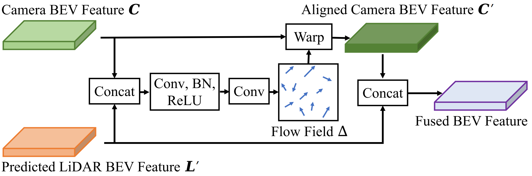
Figure 4: BEV Alignment and Fusion Module.

So far, we get both the camera and LiDAR BEV features from different branches, which usually have misalignment due to the depth estimation error and inaccurate extrinsic parameters. Therefore, direct concatenating these two BEV features will result in inferior performance. To better align BEV features, we fuse them at the BEV level and design an alignment and fusion module, as shown in Fig. 4. It takes the camera and LiDAR BEV features as input and outputs a flow field $\mathbf{\Delta}\in\mathbb{R}^{W\times H\times 2}$ for the camera BEV features. The flow field is used to warp the original camera BEV features $\mathbf{{C}}$ to the aligned BEV features $\mathbf{{C^{\prime}}}$ with LiDAR features $\mathbf{{L^{\prime}}}$. Following [19, 23], we define the warp function as

$$\mathbf{C^{\prime}}_{wh}= \mathop{\sum}\limits_{w^{\prime}=1}^{W}\mathop{\sum}\limits_{h^{\prime}=1}^{H}\mathbf{C}_{w^{\prime}h^{\prime}}\cdot\max(0,1-|w+\Delta_{1wh}-w^{\prime}|)$$

$$\cdot\max(0,1-|h+\Delta_{2wh}-h^{\prime}|)\text{,}$$ (3)

where a bilinear interpolation kernel is used to sample feature on position $(w+\Delta_{1wh},h+\Delta_{2wh})$ of $\mathbf{C}$. $\Delta_{1wh},\Delta_{2wh}$ indicate the learned 2D flow field for position $(w,h)$.

Finally, $\mathbf{{C^{\prime}}}$ and $\mathbf{{L^{\prime}}}$ are concatenated to generate the fused BEV features, which are the input of the HD map decoder.

3.4 HD Map Decoder and Training Losses

Following HDMapNet [22], we define the HD map decoder as a fully convolutional network [33] that inputs the fused BEV features and outputs three predictions, including semantic segmentation, instance embedding, and lane direction, which are then used in the post-processing step to vectorize the map.

For training three different heads for three outputs, we use different training losses. We use the cross-entropy loss $L_{seg}$ to supervise the semantic segmentation. For the instance embedding prediction, we define the loss $L_{ins}$ as a variance and a distance loss [9] as

$$L_{var}=\frac{1}{C}\sum^{C}_{c=1}\frac{1}{N_{c}}\sum^{N_{c}}_{j=1}[\|\mu_{c}-f^{\mathrm{instance}}_{j}\|-\delta_{v}]_{+}^{2},\;\;\;\;$$ (4)

$$L_{dist}=\frac{1}{C(C-1)}\sum_{c_{A}\neq c_{B}\in C}[2\delta_{d}-\|\mu_{c_{A}}-\mu_{c_{B}}\|]_{+}^{2},$$ (5)

$$L_{ins}=\alpha L_{var}+\beta L_{dist},$$ (6)

where $C$ is the number of clusters, $N_{c}$ and $\mu_{c}$ are the number of elements in cluster $c$ and mean embedding of $c$. $f^{\mathrm{instance}}_{j}$ is the embedding of the ${j}$ th element in $c$. $\|\cdot\|$ is the $L_{2}$ norm, $[x]_{+}=max(0,x)$, $\delta_{v}$ and $\delta_{d}$ are margins for the variance and distance loss.

For direction prediction, we discretize the direction into $36$ classes uniformly on a circle and define the loss $L_{dir}$ as the cross-entropy loss. We only do backpropagation for those pixels lying on the lanes that have valid directions. During inference, DBSCAN [10] is used to cluster instance embeddings, followed by non-maximum suppression [22] to reduce redundancy. We then use the predicted directions to connect the pixels greedily to get the final vector representations of HD map elements.

We use focal loss [27] with $\gamma=2.0$ for depth prediction as $L_{dep}$. The final loss is the combination of the depth estimation, semantic segmentation, instance embedding and lane direction prediction, which is defined as

$$L=\lambda_{dep}L_{dep}+\lambda_{seg}L_{seg}+\lambda_{ins}L_{ins}+\lambda_{dir}L_{dir},$$ (7)

where $\lambda_{dep}$, $\lambda_{seg}$, $\lambda_{ins}$, and $\lambda_{dir}$ are weighting factors.

4 Experiments

We evaluate SuperFusion for the long-range HD map generation task on nuScenes [4] and a self-collected dataset.

4.1 Implementation Details

Model. We use ResNet-101 [17] as our camera branch backbone and PointPillars [21] as our LiDAR branch backbone. For depth estimation, we modify DeepLabV3 [6] to generate pixel-wise probability distribution of depth bins. The camera backbone is initialized using the DeepLabV3 [6] semantic segmentation model pre-trained on the MS-COCO dataset [28]. All other components are randomly initialized. We set the image size to $256\times 704$ and voxelize the LiDAR point cloud with $0.15$ m resolution. We use $[0,90]$ m $\times$ $[-15,15]$ m as the range of the BEV HD maps, which results in a size of $600\times 200$. We set the discretized depth bins to $2.0\,\text{--}\,90.0$ m spaced by $1.0$ m.

Training Details. We train the model for $30$ epochs using stochastic gradient descent with a learning rate of 0.1. For the instance embedding, we set $\alpha=\beta=1$, $\delta_{d}=3.0$, and $\delta_{v}=0.5$. We set $\lambda_{dep}=1.0$, $\lambda_{seg}=1.0$, $\lambda_{ins}=1.0$, and $\lambda_{dir}=0.2$ for different weighting factors.

4.2 Evaluation Metrics

Intersection over Union. The IoU between the predicted HD map $M_{1}$ and ground-truth HD map $M_{2}$ is given by

$$\mathrm{IoU}(M_{1},M_{2})=\frac{|M_{1}\cap M_{2}|}{|M_{1}\cup M_{2}|}.$$ (8)

One-way Chamfer Distance. The one-way Chamfer distance (CD) between the predicted curve and ground-truth curve is given by

$$\mathrm{CD} =\frac{1}{C_{1}}\sum_{x\in C_{1}}\min_{y\in C_{2}}\|x-y\|_{2},$$ (9)

where $C_{1}$ and $C_{2}$ are sets of points on the predicted curve and ground-truth curve. CD is used to evaluate the spatial distances between two curves. There is a problem when using CD alone for the HD map evaluation. A smaller IoU tends to result in a smaller CD. We give more explanation and results on CD in the supplementary material. Here, we combine CD with IoU for selecting true positives as below to better evaluate the HD map generation task.

Average Precision. The average precision (AP) measures the instance detection capability and is defined as

$$\mathrm{AP}=\frac{1}{10}\sum_{r\in\{0.1,0.2,...,1.0\}}\mathrm{AP}_{r},$$ (10)

where $\mathrm{AP}_{r}$ is the precision at recall = $r$. As introduced in [22], they use CD to select the true positive instances. Besides that, here we also add an IoU threshold. The instance is considered as a true positive if and only if the CD is below and the IoU is above the defined thresholds. We set the threshold of IoU as 0.1 and threshold of CD as 1.0 m.

Evaluation on Multiple Intervals. To evaluate the long-range prediction ability of different methods, we split the ground truth into three intervals: $0\,\text{--}\,30$ m, $30\,\text{--}\,60$ m, and $60\,\text{--}\,90$ m. We calculate the IoU, CD, and AP of different methods on three intervals to thoroughly evaluate the HD map generation results.

4.3 Evaluation Results

nuScenes Dataset. We first evaluate our approach on the publicly available nuScenes dataset [4]. We focus on semantic HD map segmentation and instance detection tasks as introduced in [22] and consider three static map elements, including lane boundary, lane divider, and pedestrian crossing. Tab. 1 shows the comparisons of the IoU scores of semantic map segmentation. Our SuperFusion achieves the best results in all cases and has significant improvements on all intervals (Fig. 5), which shows the superiority of our method. Besides, we can observe that the LiDAR-camera fusion methods are generally better than LiDAR-only or camera-only methods. The performance of the LiDAR-only method drops quickly for long-range distances, especially for $60\,\text{--}\,90$ m, which reflects the case we analyzed in Fig. 3(a). The AP results considering both IoU and CD to decide the true positive show a more comprehensive evaluation. As shown in Tab. 2, our method achieves the best instance detection AP results for all cases with a large margin, verifying the effectiveness of our proposed novel fusion network.

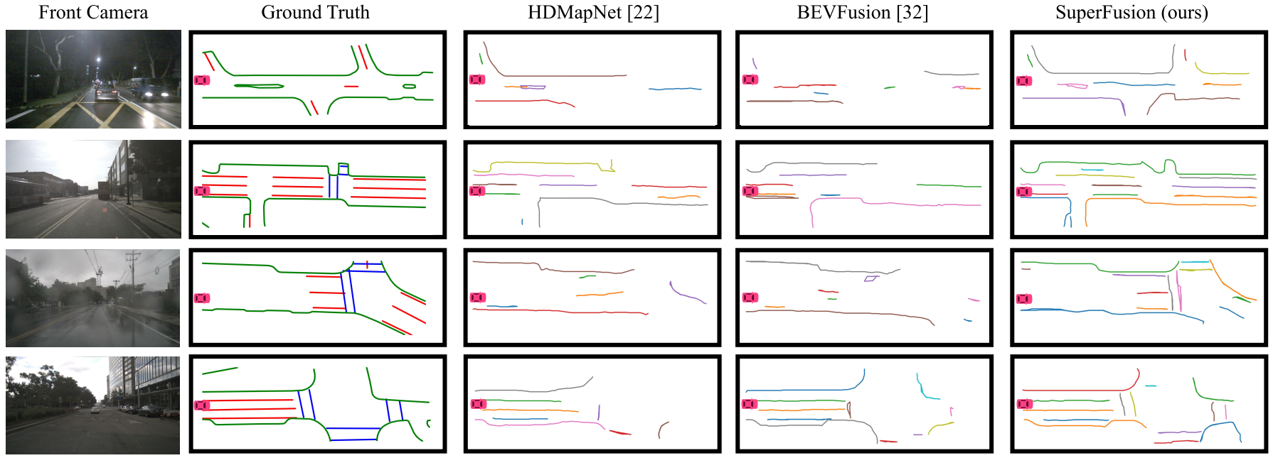
Figure 5: Qualitative HD map prediction results of different methods. The red car represents the current position of the car. The vertical length of every map is 90 m with respect to the car. Different colors indicate different HD map element instances. For ground truth HD map, green is lane boundary, red is lane divider, and blue is pedestrian crossing.

Table 1: IoU scores (%) of HD map semantic segmentation on nuScenes dataset. IoU: higher is better. C: camera. L: LiDAR.

Method	Modality	0-30 m			30-60 m			60-90 m			Average IoU
		Divider	Ped	Boundary	Divider	Ped	Boundary	Divider	Ped	Boundary	Divider	Ped	Boundary
VPN [42]	C	21.1	6.7	20.1	20.9	5.1	20.3	15.9	1.9	14.7	19.4	4.9	18.5
LSS [43]	C	35.1	16.0	33.1	28.5	6.5	26.7	22.2	2.7	20.7	28.9	9.4	27.2
PointPillars [21]	L	41.5	26.4	53.6	18.4	9.1	25.1	4.4	1.7	6.2	23.7	14.5	30.7
HDMapNet [22]	C+L	44.3	28.9	55.4	26.9	10.4	31.0	18.1	5.3	18.3	30.5	16.6	35.7
BEVFusion [26]	C+L	42.0	27.6	52.4	26.8	11.9	30.3	18.1	3.3	15.9	30.0	16.3	34.2
BEVFusion [32]	C+L	45.9	31.2	57.0	30.6	13.7	34.3	22.4	5.0	21.7	33.9	18.8	38.8
SuperFusion (ours)	C+L	47.9	37.4	58.4	35.6	22.8	39.4	29.2	12.2	28.1	38.0	26.2	42.7

Table 2: Instance detection results on nuScenes dataset. The predefined threshold of Chamfer distance is 1.0 m and the threshold of IoU is 0.1 (e.g. a prediction is considered as a true positive if and only if the CD is below and the IoU is above the defined thresholds). AP: higher is better.

Method	Modality	0-30 m			30-60 m			60-90 m			Average AP
		Divider	Ped	Boundary	Divider	Ped	Boundary	Divider	Ped	Boundary	Divider	Ped	Boundary
VPN [42]	C	16.2	3.4	30.5	17.1	4.1	30.2	13.3	1.5	21.1	15.6	3.1	27.5
LSS [43]	C	24.0	9.9	39.3	23.9	5.7	38.1	19.2	2.2	26.2	22.5	6.2	34.8
PointPillars [21]	L	24.6	18.7	49.3	15.9	7.8	36.8	4.1	1.9	9.2	15.6	10.1	32.7
HDMapNet [22]	C+L	30.5	20.0	54.5	23.7	9.2	46.3	15.2	4.2	26.4	23.6	11.7	43.1
BEVFusion [26]	C+L	25.8	19.1	47.6	20.3	10.2	38.3	12.5	4.0	18.5	20.0	11.6	35.4
BEVFusion [32]	C+L	29.7	22.5	53.6	25.1	11.5	46.1	17.9	4.8	26.9	24.7	13.6	42.8
SuperFusion (ours)	C+L	33.2	26.4	58.0	30.7	18.4	52.7	24.1	10.7	38.2	29.7	19.2	50.1

Self-recorded Dataset. To test the good generalization ability of our method, we collect our own dataset in real driving scenes and evaluate all baseline methods on that dataset. Our dataset has a similar setup as nuScenes with a LiDAR and camera sensor configuration. The static map elements are labeled by hand, including the lane boundary and lane divider. There are $21\,000$ frames of data, with $18\,000$ for training and $3\,000$ for testing. Tab. 3 shows the comparison results of different baseline methods operating on our dataset. We see consistent superior results of our method in line with those on nuScenes. Our SuperFusion outperforms the state-of-the-art methods for all cases with a large improvement. We put more details of our dataset and evaluation results on multiple intervals in the appendix.

Table 3: The average experimental results on self-recorded dataset.

Method	Modality	Average IoU		Average AP
		Divider	Boundary	Divider	Boundary
VPN [42]	C	42.9	17.9	33.0	25.4
LSS [43]	C	49.2	20.4	40.4	26.5
PointPillars [21]	L	36.8	15.5	26.1	24.6
HDMapNet [22]	C+L	46.6	18.8	38.3	25.7
BEVFusion [26]	C+L	48.1	21.9	38.8	30.5
BEVFusion [32]	C+L	49.0	18.8	40.5	25.9
SuperFusion (ours)	C+L	53.0	24.7	42.4	35.0

Table 4: Ablation of the proposed network components.

	Average IoU
	Divider	Ped	Boundary
w/o Depth Supervision	25.4	13.3	30.8
w/o Depth Prior	34.3	20.5	39.3
w/o LiDAR Prediction	33.4	17.6	38.6
w/o Cross-Attention	32.4	15.2	37.6
w/o BEV Alignment	33.4	21.8	39.1
SuperFusion (ours)	38.0	26.2	42.7

Table 5: IoU scores (%) of HD map generation in turning scenes on nuScenes dataset. We compare the results of HDMapNet and ours and show our performance improvement. Bold numbers are the best performance, and red numbers indicate larger improvements.

	Method	0-30 m			30-60 m			60-90 m			Average IoU
		Divider	Ped	Boundary	Divider	Ped	Boundary	Divider	Ped	Boundary	Divider	Ped	Boundary
original	HDMapNet [22]	44.3	28.9	55.4	26.9	10.4	31.0	18.1	5.3	18.3	30.5	16.6	35.7
	SuperFusion (ours)	47.9	37.4	58.4	35.6	22.8	39.4	29.2	12.2	28.1	38.0	26.2	42.7
	Improvement	+3.6	+8.5	+3.0	+8.7	+12.4	+8.4	+11.1	+6.9	+9.8	+7.5	+9.6	+7.0
only turns	HDMapNet [22]	42.8	27.8	53.9	24.6	10.2	27.6	17.1	4.3	16.0	29.2	14.4	32.7
	SuperFusion (ours)	46.5	37.0	57.6	33.5	22.7	38.5	28.4	11.9	26.4	36.8	24.5	40.9
	Improvement	+3.7	+9.2	+3.7	+8.9	+12.5	+10.9	+11.3	+7.6	+10.4	+7.6	+10.1	+8.2

Table 6: Module alternatives study.

Modules	Alternatives	Average IoU
		Divider	Ped	Boundary
Alignment module	DynamicAlign [26]	33.8	19.8	38.8
	ConvAlign [32]	33.5	22.9	39.1
	BEVAlign (ours)	38.0	26.2	42.7
Depth prediction module	Depth Encoder (bin)	31.2	18.5	36.1
	Depth Encoder	34.6	20.5	38.5
	Depth Channel (bin)	31.3	16.5	37.0
	Depth Channel (ours)	38.0	26.2	42.7

4.4 Ablation Studies and Module Analysis

Ablation on Each Module. We conduct ablation studies to validate the effectiveness of each component of our proposed fusion network in Tab. 4. Without depth supervision, the inaccurate depth estimation influences the camera-to-BEV transformation and makes the following alignment module fails, which results in the worst performance. Without the sparse depth map prior from the LiDAR point cloud, the depth estimation is unreliable under challenging environments and thus produces inferior results. Without the prediction module, there is no measurement from LiDAR in the long-range interval, and only camera information is useful, thus deteriorating the overall performance. In the ”w/o Cross Attention” setting, we add the encoder-decoder LiDAR BEV prediction structure but remove the cross-attention interaction with camera FV features. In this case, the network tries to learn the LiDAR completion from the data implicitly without guidance from images. The performance drops significantly for this setup, indicating the importance of our proposed image-guided LiDAR prediction module. In the last setting, we remove the BEV alignment module and concatenate the BEV features from the camera and LiDAR directly. As can be seen, due to inaccurate depth estimation and extrinsic parameters, the performance without an alignment is worse than using our proposed BEV aligning module.

Analysis of Module Choices. In the upper part of Tab. 6, we show that our BEVAlign module works better than the alignment methods proposed in the previous work [32, 26]. [32] uses a simple convolution-based encoder for alignment, which is not enough when the depth estimation is inaccurate. The dynamic fusion module proposed in  [26] works well on 3D object detection tasks but has a limitation on semantic segmentation tasks.

In the lower part of Tab. 6, we test different ways to add depth prior. One way is to add the sparse depth map as an additional input channel for the image branch. Another way is to use a lightweight encoder separately on RGB image and sparse depth map and concatenate the features from the encoder as the input for the image branch. Besides, the sparse depth map can either store the original depth values or the bin depth values. We see that adding the sparse depth map as an additional input channel with original depth values achieves the best performance.

4.5 Insights and Applications

This section provides more insights into the performance of our method on long-range distance HD map generation and shows such good long-range distance HD map generation is important to downstream path planning and motion control applications for autonomous driving.

HD Map Generation in Turning Scenes. This experiment shows the advantage of our method for long-range HD map generation in the turning scenes, which is essential to downstream path planning since better predicting the turns leads to smoother paths. We select all the turning cases in the nuScenes [4] validation set and evaluate the turn samples separately. As shown in Tab. 5, compared to the HDMapNet [22], the improvement of our method is further increased for the turning scenes, which indicates that our method better predicts the turns.

Useful for Path Planning. We use the same dynamic window approach (DWA) [12] for path planning on HD maps generated by HDMapNet [22], BEVFusion [32], and our SuperFusion. We randomly select $100$ different scenes and one drivable point between $30\,\text{--}\,90$ m as the goal for each scene. The planning is failed if the path intersects with the sidewalk or DWA fails to plan a valid path. Tab. 7 shows the planning success rate for different methods. As can be seen, benefiting from accurate prediction for long-range and turning cases, our method has significant improvement compared to the baselines. Fig. 6 shows more visualizations of the planning results.

Table 7: Quantitative path planning results.

	HDMapNet [22]	BEVFusion [32]	SuperFusion (ours)
Success rate	45%	49%	72%

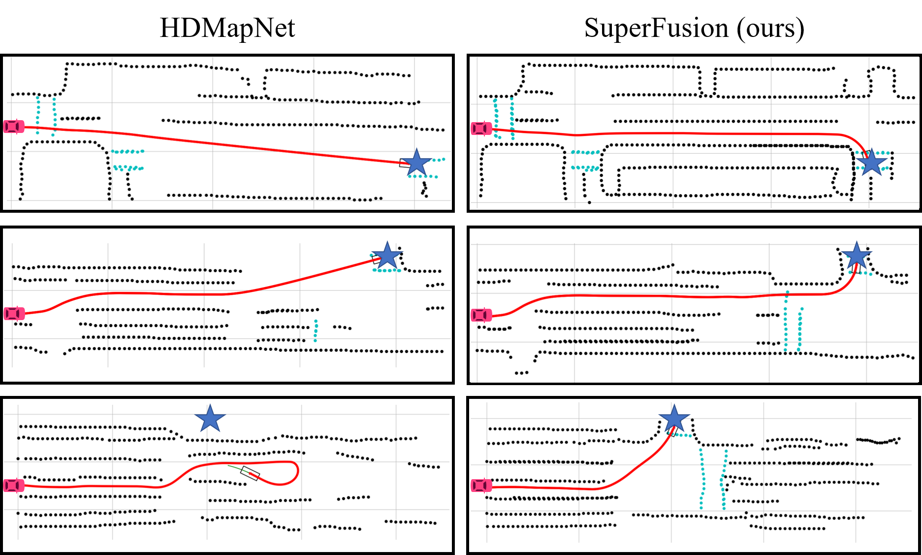
Figure 6: Path planning results on the generated HD maps.

5 Conclusion

In this paper, we proposed a novel LiDAR-camera fusion network named SuperFusion to tackle the long-range HD map generation task. It exploits the fusion of LiDAR and camera data at multiple levels and generates accurate HD maps in long-range distances up to 90 m. We thoroughly evaluate our SuperFusion on the nuScenes dataset and our self-recorded dataset in autonomous driving environments. The experimental results show that our method outperforms the state-of-the-art methods in HD map generation with large margins. We furthermore provided our insights and showed that the long-range HD maps generated by our method are more beneficial for downstream path planning tasks.

Limitation. Despite significant improvement achieved by our SuperFusion, one potential limitation of our method is that it relies on both LiDAR and camera sensor data, thus degrading performance when one of the data is missing. In real applications, we can use a multi-thread framework [45] to tackle this problem and improve its robustness.

Societal Impacts. Online local HD map generation will largely improve the robustness and safety of autonomous vehicles. Our SuperFusion can accurately generate HD maps for long-range distances, allowing planning algorithms to plan earlier and better avoid slowly moving pedestrians like older people or baby strollers.

A More Network Architecture Details

A.1 LiDAR BEV Prediction Module

Our proposed BEV prediction module is an encoder-decoder network. Tab. 8 and Tab. 9 show the architecture parameters of our encoder and decoder. The input to the encoder is the original LiDAR BEV feature $\mathbf{{L}}$ of size ${200\times 600\times 128}$, and the output is the bottleneck feature $\mathbf{{B}}$ of size ${50\times 150\times 256}$. Then, a cross-attention mechanism is applied to dynamically capture the correlations between $\mathbf{{B}}$ and FV image feature $\mathbf{{F}}$ and finally get the bottleneck feature $\mathbf{{B^{\prime}}}$ with the visual guidance from images. The decoder takes $\mathbf{{B^{\prime}}}$ as input and outputs the predicted LiDAR BEV feature $\mathbf{{L^{\prime}}}$ of size ${200\times 600\times 128}$.

A.2 BEV Alignment Module

Tab. 10 shows the architecture of the BEV alignment module. It takes the concatenation of camera and LiDAR BEV features as input and outputs a flow field $\mathbf{\Delta}$ with the size of ${200\times 600\times 2}$. The flow field is then used to warp the original camera BEV features $\mathbf{{C}}$ to the aligned features $\mathbf{{C^{\prime}}}$ with respect to LiDAR features $\mathbf{{L^{\prime}}}$.

Table 8: Layers of LiDAR BEV prediction encoder

Operator	Stride	Filters	Kernal Size	Padding	Output Shape
Conv2D	1	256	3	1	$200\times 600\times 256$
BN+ReLU	-	-	-	-	$200\times 600\times 256$
MaxPool2D	2	-	2	-	$100\times 300\times 256$
Conv2D	1	256	3	1	$100\times 300\times 256$
BN+ReLU	-	-	-	-	$100\times 300\times 256$
MaxPool2D	2	-	2	-	$50\times 150\times 256$
Conv2D	1	256	3	1	$50\times 150\times 256$
BN+ReLU	-	-	-	-	$50\times 150\times 256$

Table 9: Layers of LiDAR BEV prediction decoder

Operator	Stride	Filters	Kernal Size	Padding	Output Shape
Conv2D	1	256	3	1	$50\times 150\times 256$
BN+ReLU	-	-	-	-	$50\times 150\times 256$
MaxUnpool2d	2	-	2	-	$100\times 300\times 256$
Conv2D	1	256	3	1	$100\times 300\times 256$
BN+ReLU	-	-	-	-	$100\times 300\times 256$
MaxUnpool2d	2	-	2	-	$200\times 600\times 256$
Conv2D	1	128	3	1	$200\times 600\times 128$

Table 10: Layers of BEV alignment module

Operator	Stride	Filters	Kernal Size	Padding	Output Shape
Conv2D	1	128	1	-	$200\times 600\times 128$
BN+ReLU	-	-	-	-	$200\times 600\times 128$
Conv2D	1	2	3	1	$200\times 600\times 2$

B Evaluation Metrics

The typical Chamfer distance (CD) is bi-directional. The CD between the predicted curve and the ground-truth curve is given by

$$\mathrm{CD}=\mathrm{CD_{pred}}+\mathrm{CD_{gt}},$$ (11)

$$\mathrm{CD_{pred}}=\frac{1}{C_{1}}\sum_{x\in C_{1}}\min_{y\in C_{2}}\|x-y\|_{2},$$ (12)

$$\mathrm{CD_{gt}}=\frac{1}{C_{2}}\sum_{x\in C_{2}}\min_{y\in C_{1}}\|x-y\|_{2},$$ (13)

where $C_{1}$ and $C_{2}$ are set of points on the predicted curve and ground-truth curve. We provide one example in Fig. 7 to show that using the typical CD alone cannot well represent the quality of HD map generation. To calculate $\mathrm{CD_{pred}}$, we sample points with an equal interval from the predicted curve. We select the nearest point on the ground-truth curve for each sampled point and calculate the distance. In this case, the average of the yellow arrows shown in Fig. 7 is $\mathrm{CD_{pred}}$. The calculation of $\mathrm{CD_{gt}}$ is inverse. We sample points with an equal interval from the ground-truth curve. For each sampled point, we find the nearest point on the predicted curve and calculate the distance. In this case, the average of the blue arrows shown in Fig. 7 is $\mathrm{CD_{gt}}$. When the IoU is relatively small, which is a frequent case for long-range predictions, although the predicted curve and ground-truth curve are very close, the $\mathrm{CD_{gt}}$ will still be very large. As a result, $\mathrm{CD}$ will also be very large. Therefore, $\mathrm{CD}$ cannot represent the real performance of different methods, thus not a good metric to evaluate the spatial distances between two curves for the long-range HD map generation task. As shown in Tab. 11, $\mathrm{CD}$ becomes very large for $60\,\text{--}\,90$ m due to a relatively low IoU prediction. However, the prediction and the ground truth may already be very close. $\mathrm{CD_{pred}}$ can better evaluate the spatial distances between two curves even if the IoU is small. However, a smaller IoU still tends to result in a smaller $\mathrm{CD_{pred}}$ since fewer points are sampled and evaluated. Hence, we provide the results of $\mathrm{CD}$ in the supplementary just for reference and combine $\mathrm{CD_{pred}}$ and IoU to calculate AP to better evaluate the HD map generation task.

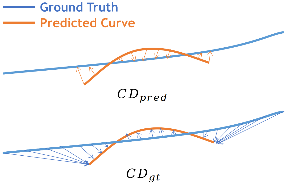
Figure 7: The illustration on the calculation of $\mathrm{CD_{pred}}$ and $\mathrm{CD_{gt}}$.

C Self-recorded Dataset

The dataset is recorded using a multi-sensor setup, including a front-view camera and two 128-beam RoboSense M1 LiDARs. One LiDAR is put on the front left of the car and another on the front right. The data from two LiDARs are merged using extrinsic parameters to generate the front-view point clouds. The data is recorded in a city road environment with 10 km distances. The dataset is recorded on multiple streets in a large city with significant visual differences as shown in Fig. 8(c). There are $21\,000$ frames of annotated data, with $18\,000$ for training and $3\,000$ for testing. The static map elements, including lane boundary and lane divider, are labeled by hand using the intensity information from LiDAR and verified using camera data. The point clouds are concatenated in order to label long-range distances up to 90 m. Fig. 8 shows some example data from nuScenes and our self-recorded datasets. Due to different cities, road styles, and weather conditions, we can easily see the difference between these two datasets from the image and LiDAR data. Since the LiDAR sensors are also different, the LiDAR data have large diversity between these two datasets. Besides, the extrinsic parameters between the camera and LiDAR and the camera intrinsic parameters of our self-recorded dataset are also different from the nuScenes dataset. Therefore, our self-recorded dataset is dissimilar enough compared to the nuScenes dataset to verify the robustness and generalization ability of different methods under different types of input. Our self-recorded dataset will be released to public for long-range HD map generation research.

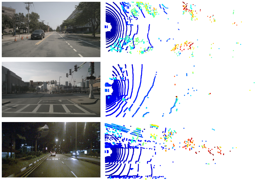
(a) Sample images and LiDAR data from nuScenes dataset.

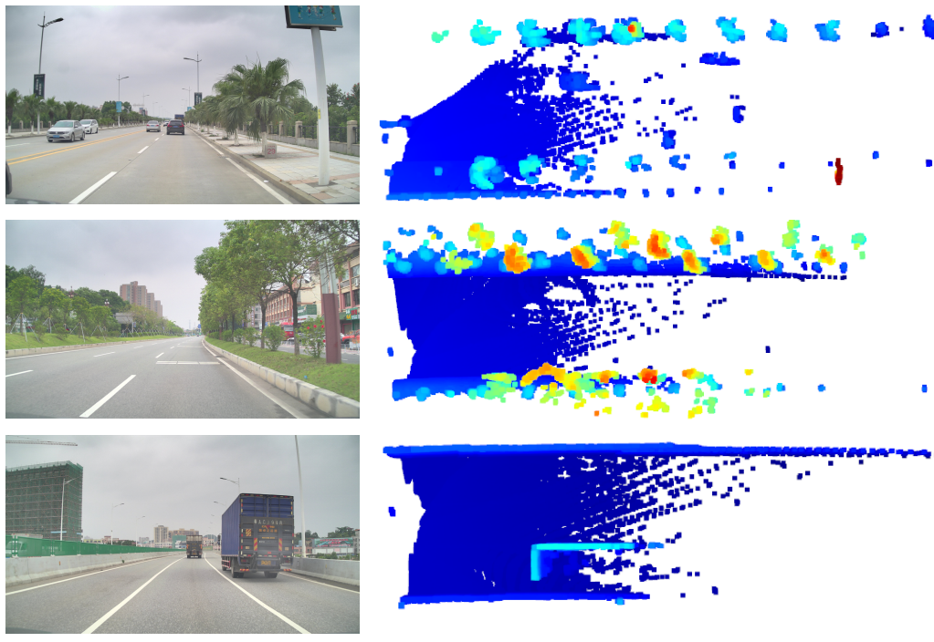
(b) Sample images and LiDAR data from self-recorded dataset.

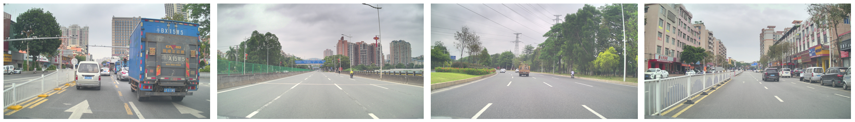
(c) More examples on self-recorded dataset.

Figure 8: Sample data from nuScenes and self-recorded datasets.

D Additional Experimental Results

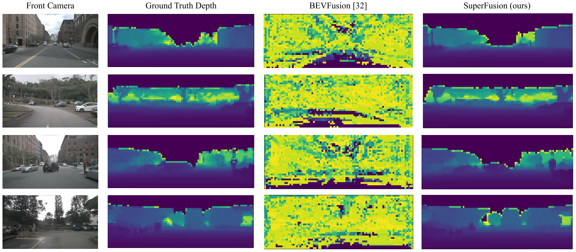
Figure 9: Depth distribution prediction examples. Benefiting from depth supervision and prior, our method can accurately estimate the depth distribution.

Depth Distribution Prediction. Fig. 9 shows the depth prediction results from the Camera-to-BEV transformation module. Accurate depth estimation is essential to lift the image into a frustum of features. Both BEVFusion [32] and our method estimate a categorical depth distribution, but using different methods. The depth prediction module in BEVFusion [32] is only implicitly supervised by the semantic segmentation loss, which is insufficient to generate accurate depth estimation and suffers from smearing effects. Instead, our method uses both the completed dense LiDAR depth image for supervision and also the sparse depth image as an additional channel to the RGB image. In this way, our network exploits both a depth prior and an accurate depth supervision, thus generalizing well to different challenging environments and can estimate the depth distribution accurately, as shown in Fig. 9. This is also one of the reasons why our method significantly improved compared to the baseline methods, which is consistent with our ablation studies shown in the main paper.

Temporal Consistency Results. Fig. 10 shows the HD map predictions of five consecutive frames using different methods. The HD maps generated by our method show strong consistency compared to the baselines. The consistent and stable prediction of the HD maps are crucial to downstream path planning and motion control applications for autonomous driving.

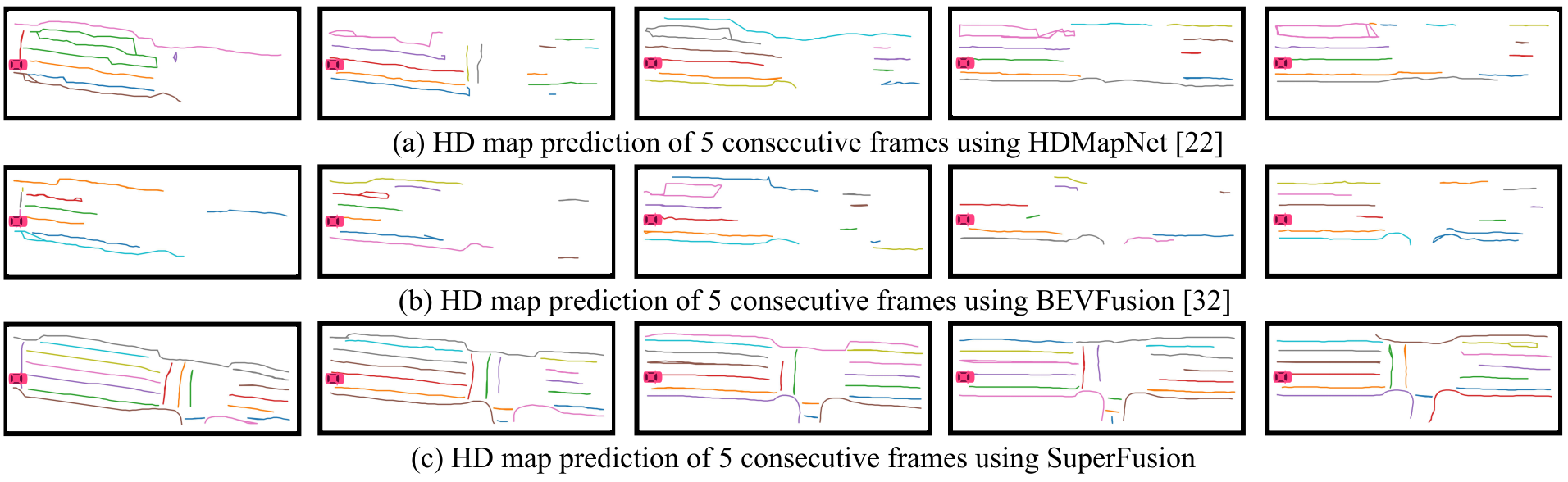
Figure 10: Temporal consistency of the generated HD maps.

CD results. Tab. 11 shows the Chamfer distance results of semantic map segmentation on nuScenes dataset. Our SuperFusion also achieves the best results in all cases and has significant improvements, which shows the advantage of our method. We can observe that $\mathrm{CD}$ becomes very large for $60\,\text{--}\,90$ m due to a relatively low IoU prediction. As analyzed in Sec. B, $\mathrm{CD}$ is not a good metric to evaluate the spatial distances alone between two curves for long-range HD map generation task. Therefore, we provide the results of $\mathrm{CD}$ in the supplementary just for reference and use AP in the main paper as a more comprehensive evaluation metric for different methods.

More results on the self-recorded dataset. Tab. 12 to Tab. 14 show the detailed comparison results of different baseline methods with different intervals operating on our self-recorded dataset. We see consistent superior results of our method in line with those on nuScenes. Our SuperFusion outperforms the state-of-the-art methods in most cases with a significant improvement.

More qualitative results. Fig. 11 and Fig. 12 show more qualitative HD map prediction results on nuScenes and our self-recorded datasets. Our method has impressive results compared to baselines, especially in long-range distances and under bad weather conditions. Besides, our method can detect turning cases more accurately, which benefits downstream path planning tasks.

Table 11: Chamfer distance (m) of semantic map segmentation on nuScenes dataset. CD: lower is better.

Method	Modality	0-30 m			30-60 m			60-90 m			Average CD
		Divider	Ped	Boundary	Divider	Ped	Boundary	Divider	Ped	Boundary	Divider	Ped	Boundary
VPN [42]	C	3.212	4.521	3.279	2.970	4.734	2.814	2.998	5.000	3.622	3.066	4.729	3.217
LSS [43]	C	2.123	3.168	2.043	2.376	4.908	2.426	2.409	5.000	3.033	2.290	4.223	2.454
PointPillars [21]	L	1.691	2.661	0.929	4.049	4.646	3.503	5.000	4.958	5.000	3.515	3.818	3.190
HDMapNet [22]	C+L	1.473	2.284	0.779	2.456	4.210	1.947	2.905	5.000	3.466	2.185	3.598	1.869
BEVFusion [26]	C+L	1.702	2.283	1.212	2.816	4.237	2.929	3.490	5.000	4.915	2.534	3.588	2.701
BEVFusion [32]	C+L	1.384	2.036	0.773	2.523	3.762	2.106	3.102	5.000	3.754	2.213	3.282	1.980
SuperFusion (ours)	C+L	1.305	1.503	0.542	1.756	2.641	1.235	1.964	4.081	2.221	1.642	2.449	1.228

Table 12: IoU scores (%) of semantic map segmentation on self-recorded dataset. IoU: higher is better.

Method	Modality	0-30 m		30-60 m		60-90 m		Average IoU
		Divider	Boundary	Divider	Boundary	Divider	Boundary	Divider	Boundary
VPN [42]	C	49.6	21.6	46.3	18.4	33.1	13.6	42.9	17.9
LSS [43]	C	52.3	22.1	52.2	21.5	43.5	17.4	49.2	20.4
PointPillars [21]	L	46.7	20.1	39.4	16.0	25.2	8.8	36.8	15.5
HDMapNet [22]	C+L	54.6	22.5	50.8	19.5	35.0	14.0	46.6	18.8
BEVFusion [26]	C+L	53.1	26.4	50.1	21.9	41.7	17.2	48.1	21.9
BEVFusion [32]	C+L	51.9	21.4	51.7	20.0	43.6	15.3	49.0	18.8
SuperFusion (ours)	C+L	59.9	28.4	55.2	25.2	44.2	20.4	53.0	24.7

Table 13: Chamfer distance (m) of semantic map segmentation on self-recorded dataset. CD: lower is better.

Method	Modality	0-30 m		30-60 m		60-90 m		Average CD
		Divider	Boundary	Divider	Boundary	Divider	Boundary	Divider	Boundary
VPN [42]	C	1.058	3.280	1.298	3.980	2.657	4.501	1.638	3.915
LSS [43]	C	1.067	3.579	1.048	4.074	2.412	5.000	1.244	4.111
PointPillars [21]	L	1.243	3.379	1.856	5.000	3.862	5.000	1.752	4.512
HDMapNet [22]	C+L	0.906	3.379	1.065	3.807	2.478	4.161	1.444	3.770
BEVFusion [26]	C+L	1.054	3.035	0.975	3.488	1.553	3.875	1.188	3.578
BEVFusion [32]	C+L	1.071	3.504	1.022	3.745	1.447	4.436	1.176	3.887
SuperFusion (ours)	C+L	0.834	2.992	0.851	2.988	1.543	3.824	1.066	3.256

Table 14: Instance detection results on self-recorded dataset. The predefined threshold of Chamfer distance is 1.0 m and threshold of IoU is 0.1 (e.g. a prediction is considered as a true positive if and only if the CD is below and the IoU is above the defined thresholds). AP: higher is better.

Method	Modality	0-30 m		30-60 m		60-90 m		Average AP
		Divider	Boundary	Divider	Boundary	Divider	Boundary	Divider	Boundary
VPN [42]	C	40.9	28.9	36.2	27.1	21.9	20.0	33.0	25.4
LSS [43]	C	42.8	28.9	42.7	27.7	35.8	22.9	40.4	26.5
PointPillars [21]	L	30.7	29.0	28.0	27.6	19.7	17.2	26.1	24.6
HDMapNet [22]	C+L	44.9	29.2	43.0	28.1	27.1	19.9	38.3	25.7
BEVFusion [26]	C+L	42.1	34.2	40.4	31.9	33.9	25.2	38.8	30.5
BEVFusion [32]	C+L	43.0	28.8	42.6	27.5	35.9	21.4	40.5	25.9
SuperFusion (ours)	C+L	47.5	38.0	44.3	36.8	35.3	30.0	42.4	35.0

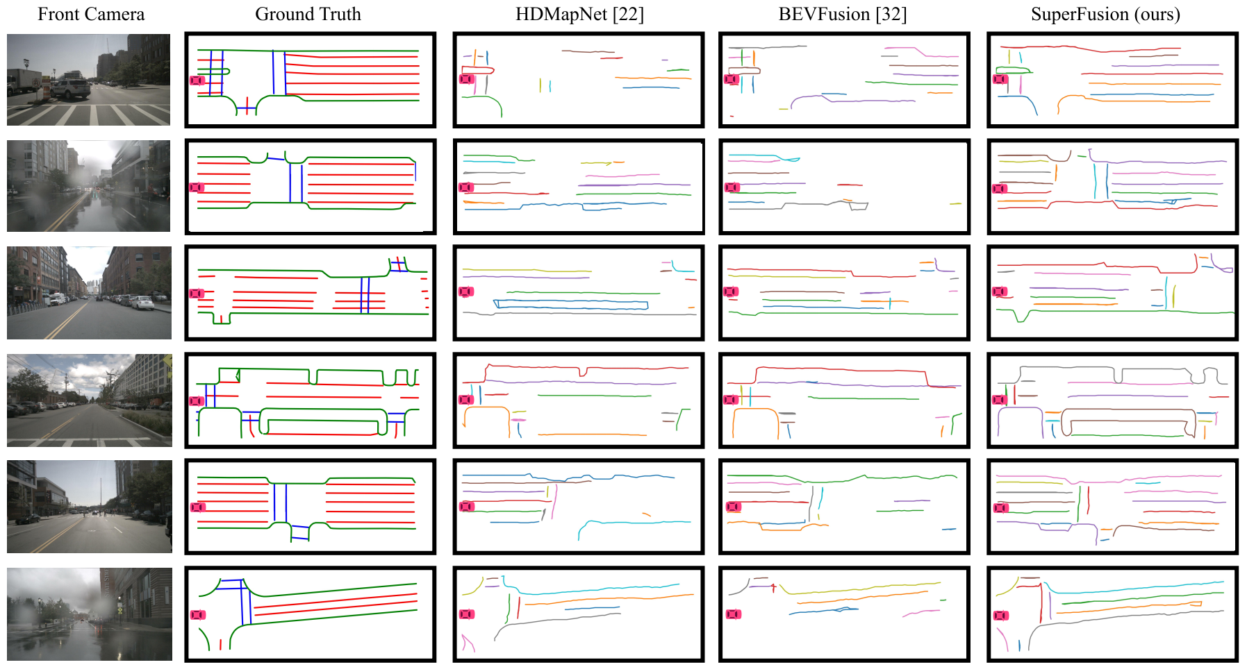
Figure 11: Qualitative HD map prediction results of different methods on nuScenes dataset. The red car represents the current position of the car. The verticle length of every map is 90 m with respect to the car. Different colors indicate different HD map element instances.

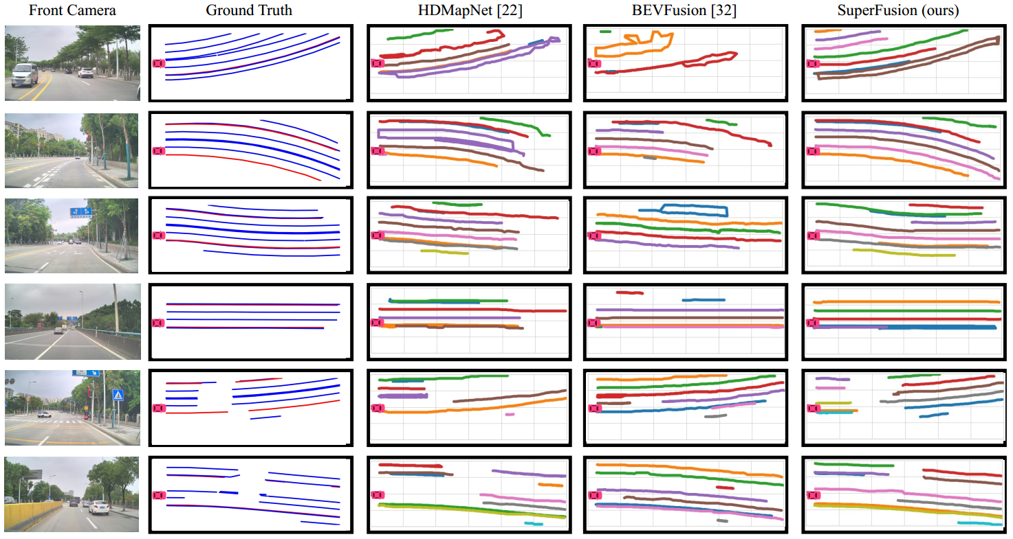
Figure 12: Qualitative HD map prediction results of different methods on self-recorded dataset. The red car represents the current position of the car. The verticle length of every map is 90 m with respect to the car. Different colors indicate different HD map element instances.

References

- [1] Syed Ammar Abbas and Andrew Zisserman. A geometric approach to obtain a bird’s eye view from an image. In ICCVW, 2019.
- [2] Xuyang Bai, Zeyu Hu, Xinge Zhu, Qingqiu Huang, Yilun Chen, Hongbo Fu, and Chiew-Lan Tai. Transfusion: Robust lidar-camera fusion for 3d object detection with transformers. In CVPR, 2022.
- [3] Alejandro Barrera, Carlos Guindel, Jorge Beltrán, and Fernando García. Birdnet+: End-to-end 3d object detection in lidar bird’s eye view. In ITSC, 2020.
- [4] Holger Caesar, Varun Bankiti, Alex H. Lang, Sourabh Vora, Venice Erin Liong, Qiang Xu, Anush Krishnan, Yu Pan, Giancarlo Baldan, and Oscar Beijbom. nuscenes: A multimodal dataset for autonomous driving. arXiv preprint arXiv:1903.11027, 2019.
- [5] Yigit Baran Can, Alexander Liniger, Ozan Unal, Danda Paudel, and Luc Van Gool. Understanding bird’s-eye view of road semantics using an onboard camera. IEEE Robotics and Automation Letters, 7(2):3302–3309, 2022.
- [6] Liang-Chieh Chen, George Papandreou, Florian Schroff, and Hartwig Adam. Rethinking atrous convolution for semantic image segmentation. arXiv preprint arXiv:1706.05587, 2017.
- [7] Li Chen, Chonghao Sima, Yang Li, Zehan Zheng, Jiajie Xu, Xiangwei Geng, Hongyang Li, Conghui He, Jianping Shi, Yu Qiao, and Junchi Yan. Persformer: 3d lane detection via perspective transformer and the openlane benchmark. In ECCV, 2022.
- [8] Xuanyao Chen, Tianyuan Zhang, Yue Wang, Yilun Wang, and Hang Zhao. Futr3d: A unified sensor fusion framework for 3d detection. arXiv preprint arXiv:2203.10642, 2022.
- [9] Bert De Brabandere, Davy Neven, and Luc Van Gool. Semantic instance segmentation for autonomous driving. In CVPRW, 2017.
- [10] Martin Ester, Hans-Peter Kriegel, Jörg Sander, and Xiaowei Xu. A density-based algorithm for discovering clusters in large spatial databases with noise. In Proceedings of the Second International Conference on Knowledge Discovery and Data Mining, page 226–231, 1996.
- [11] Sudeep Fadadu, Shreyash Pandey, Darshan Hegde, Yi Shi, Fang-Chieh Chou, Nemanja Djuric, and Carlos Vallespi-Gonzalez. Multi-view fusion of sensor data for improved perception and prediction in autonomous driving. In WACV, 2022.
- [12] D. Fox, W. Burgard, and S. Thrun. The dynamic window approach to collision avoidance. IEEE Robotics and Automation Magazine, 4(1):23–33, 1997.
- [13] Noa Garnett, Rafi Cohen, Tomer Pe’er, Roee Lahav, and Dan Levi. 3d-lanenet: end-to-end 3d multiple lane detection. In ICCV, 2019.
- [14] Farouk Ghallabi, Fawzi Nashashibi, Ghayath El-Haj-Shhade, and Marie-Anne Mittet. Lidar-based lane marking detection for vehicle positioning in an hd map. In ITSC, 2018.
- [15] Yuliang Guo, Guang Chen, Peitao Zhao, Weide Zhang, Jinghao Miao, Jingao Wang, and Tae Eun Choe. Gen-lanenet: A generalized and scalable approach for 3d lane detection. In ECCV, 2020.
- [16] Adam W. Harley, Zhaoyuan Fang, Jie Li, Rares Ambrus, and Katerina Fragkiadaki. Simple-BEV: What really matters for multi-sensor bev perception? In arXiv:2206.07959, 2022.
- [17] Kaiming He, Xiangyu Zhang, Shaoqing Ren, and Jian Sun. Deep residual learning for image recognition. In CVPR, 2016.
- [18] Anthony Hu, Zak Murez, Nikhil Mohan, Sofía Dudas, Jeffrey Hawke, Vijay Badrinarayanan, Roberto Cipolla, and Alex Kendall. FIERY: Future instance segmentation in bird’s-eye view from surround monocular cameras. In ICCV, 2021.
- [19] Zilong Huang, Yunchao Wei, Xinggang Wang, Humphrey Shi, Wenyu Liu, and Thomas S Huang. Alignseg: Feature-aligned segmentation networks. TPAMI, 2021.
- [20] Jason Ku, Ali Harakeh, and Steven L Waslander. In defense of classical image processing: Fast depth completion on the cpu. In CRV, 2018.
- [21] Alex H. Lang, Sourabh Vora, Holger Caesar, Lubing Zhou, Jiong Yang, and Oscar Beijbom. Pointpillars: Fast encoders for object detection from point clouds. arXiv preprint arXiv:1812.05784, 2019.
- [22] Qi Li, Yue Wang, Yilun Wang, and Hang Zhao. Hdmapnet: An online hd map construction and evaluation framework. arXiv preprint arXiv:2107.06307, 2021.
- [23] Xiangtai Li, Ansheng You, Zhen Zhu, Houlong Zhao, Maoke Yang, Kuiyuan Yang, and Yunhai Tong. Semantic flow for fast and accurate scene parsing. In ECCV, 2020.
- [24] Yingwei Li, Adams Wei Yu, Tianjian Meng, Ben Caine, Jiquan Ngiam, Daiyi Peng, Junyang Shen, Yifeng Lu, Denny Zhou, Quoc V Le, et al. Deepfusion: Lidar-camera deep fusion for multi-modal 3d object detection. In CVPR, 2022.
- [25] Zhiqi Li, Wenhai Wang, Hongyang Li, Enze Xie, Chonghao Sima, Tong Lu, Qiao Yu, and Jifeng Dai. Bevformer: Learning bird’s-eye-view representation from multi-camera images via spatiotemporal transformers. arXiv preprint arXiv:2203.17270, 2022.
- [26] Tingting Liang, Hongwei Xie, Kaicheng Yu, Zhongyu Xia, Zhiwei Lin, Yongtao Wang, Tao Tang, Bing Wang, and Zhi Tang. BEVFusion: A Simple and Robust LiDAR-Camera Fusion Framework. arXiv preprint arXiv:2205.13790, 2022.
- [27] T. Lin, P. Goyal, R. Girshick, K. He, and P. Dollar. Focal loss for dense object detection. TPAMI, 2020.
- [28] Tsung-Yi Lin, Michael Maire, Serge J. Belongie, Lubomir D. Bourdev, Ross B. Girshick, James Hays, Pietro Perona, Deva Ramanan, Piotr Dollár, and C. Lawrence Zitnick. Microsoft COCO: common objects in context. In ECCV, 2014.
- [29] Tsung-Yi Lin, Piotr Dollár, Ross Girshick, Kaiming He, Bharath Hariharan, and Serge Belongie. Feature pyramid networks for object detection. In CVPR, 2017.
- [30] Yicheng Liu, Yue Wang, Yilun Wang, and Hang Zhao. Vectormapnet: End-to-end vectorized hd map learning. arXiv preprint arXiv:2206.08920, 2022.
- [31] Yingfei Liu, Junjie Yan, Fan Jia, Shuailin Li, Qi Gao, Tiancai Wang, Xiangyu Zhang, and Jian Sun. Petrv2: A unified framework for 3d perception from multi-camera images. arXiv preprint arXiv:2206.01256, 2022.
- [32] Zhijian Liu, Haotian Tang, Alexander Amini, Xingyu Yang, Huizi Mao, Daniela Rus, and Song Han. Bevfusion: Multi-task multi-sensor fusion with unified bird’s-eye view representation. arXiv preprint arXiv:2205.13542, 2022.
- [33] Jonathan Long, Evan Shelhamer, and Trevor Darrell. Fully convolutional networks for semantic segmentation. In CVPR, 2015.
- [34] Abdelhak Loukkal, Yves Grandvalet, Tom Drummond, and You Li. Driving among flatmobiles: Bird-eye-view occupancy grids from a monocular camera for holistic trajectory planning. In WACV, 2021.
- [35] Chenyang Lu, Marinus Jacobus Gerardus van de Molengraft, and Gijs Dubbelman. Monocular Semantic Occupancy Grid Mapping With Convolutional Variational Encoder-Decoder Networks. IEEE Robotics and Automation Letters, 4(2):445–452, 2019.
- [36] Lun Luo, Si-Yuan Cao, Bin Han, Hui-Liang Shen, and Junwei Li. Bvmatch: Lidar-based place recognition using bird’s-eye view images. IEEE Robotics and Automation Letters, 6(3):6076–6083, 2021.
- [37] Fangchang Ma, Guilherme Venturelli Cavalheiro, and Sertac Karaman. Self-supervised sparse-to-dense: Self-supervised depth completion from lidar and monocular camera. arXiv preprint arXiv:1807.00275, 2018.
- [38] Fangchang Ma and Sertac Karaman. Sparse-to-dense: Depth prediction from sparse depth samples and a single image. In ICRA, 2018.
- [39] Yuexin Ma, Tai Wang, Xuyang Bai, Huitong Yang, Yuenan Hou, Yaming Wang, Y. Qiao, Ruigang Yang, Dinesh Manocha, and Xinge Zhu. Vision-centric bev perception: A survey. arXiv preprint arXiv:2208.02797, 2022.
- [40] Hanspeter Mallot, Heinrich Bülthoff, J.J. Little, and S Bohrer. Inverse perspective mapping simplifies optical flow computation and obstacle detection. Biological cybernetics, 64:177–85, 02 1991.
- [41] Raúl Mur-Artal and Juan D. Tardós. Orb-slam2: An open-source slam system for monocular, stereo, and rgb-d cameras. IEEE Transactions on Robotics, 33(5):1255–1262, 2017.
- [42] Bowen Pan, Jiankai Sun, Ho Yin Tiga Leung, Alex Andonian, and Bolei Zhou. Cross-view semantic segmentation for sensing surroundings. IEEE Robotics and Automation Letters, 5(3):4867–4873, Jul 2020.
- [43] Jonah Philion and Sanja Fidler. Lift, splat, shoot: Encoding images from arbitrary camera rigs by implicitly unprojecting to 3d. In ECCV, 2020.
- [44] Cody Reading, Ali Harakeh, Julia Chae, and Steven L Waslander. Categorical depth distribution network for monocular 3d object detection. In CVPR, 2021.
- [45] Andrzej Reinke, Xieyuanli Chen, and Cyrill Stachniss. Simple but effective redundant odometry for autonomous vehicles. In ICRA, 2021.
- [46] Thomas Roddick and Roberto Cipolla. Predicting semantic map representations from images using pyramid occupancy networks. In CVPR, 2020.
- [47] Avishkar Saha, Oscar Mendez, Chris Russell, and Richard Bowden. Translating images into maps. In ICRA, 2022.
- [48] Liangchen Song, Jialian Wu, Ming Yang, Qian Zhang, Yuan Li, and Junsong Yuan. Stacked homography transformations for multi-view pedestrian detection. In ICCV, 2021.
- [49] Ashish Vaswani, Noam Shazeer, Niki Parmar, Jakob Uszkoreit, Llion Jones, Aidan N. Gomez, Lukasz Kaiser, and Illia Polosukhin. Attention is all you need. In NeurIPS, 2017.
- [50] Sourabh Vora, Alex H Lang, Bassam Helou, and Oscar Beijbom. Pointpainting: Sequential fusion for 3d object detection. In CVPR, 2020.
- [51] Chunwei Wang, Chao Ma, Ming Zhu, and Xiaokang Yang. Pointaugmenting: Cross-modal augmentation for 3d object detection. In CVPR, 2021.
- [52] Hengli Wang, Peide Cai, Rui Fan, Yuxiang Sun, and Ming Liu. End-to-end interactive prediction and planning with optical flow distillation for autonomous driving. In CVPRW, 2021.
- [53] Yan Yan, Yuxing Mao, and Bo Li. Second: Sparsely embedded convolutional detection. Sensors, 18(10), 2018.
- [54] Tianwei Yin, Xingyi Zhou, and Philipp Krähenbühl. Center-based 3d object detection and tracking. In CVPR, 2021.
- [55] Brady Zhou and Philipp Krähenbühl. Cross-view transformers for real-time map-view semantic segmentation. In CVPR, 2022.
- [56] Yin Zhou, Pei Sun, Yu Zhang, Dragomir Anguelov, Jiyang Gao, Tom Ouyang, James Guo, Jiquan Ngiam, and Vijay Vasudevan. End-to-end multi-view fusion for 3d object detection in lidar point clouds. In PMLR, 2020.