Stochastic Optimal Control via Local Occupation Measures

Abstract

Viewing stochastic processes through the lens of occupation measures has proven to be a powerful angle of attack for the theoretical and computational analysis for a wide range of stochastic optimal control problems. We present a simple modification of the traditional occupation measure framework derived from resolving the occupation measures locally on a partition of the state space and control horizon. This modification bridges the gap between discretization based approximations to the solution of the Hamilton-Jacobi-Bellmann equations and convex optimization based approaches relying on the moment-sum-of-squares hierarchy. When combined with the moment-sum-of-squares hierarchy, the notion of local occupation measures provides fine-grained control over the construction of highly structured semidefinite programming relaxations for a rich class of stochastic optimal control problems with embedded diffusion and jump processes. We show how these relaxations are constructed, analyze their favorable properties, and demonstrate with examples that they hold the potential to allow for the computation of tighter bounds orders of magnitude faster than is possible via naive combination of the moment-sum-of-squares hierarchy with the traditional occupation measure framework.

1 Introduction

The optimal control of stochastic processes is arguably one of the most fundamental problems in the context of decision-making under uncertainty. While a wide range of decision-making problems in engineering lend themselves to be naturally modeled as such stochastic optimal control problems, only a small subset of them admits identification of a globally optimal control policy in a tractable and certifiable manner. As a consequence, engineers are often forced to resort to one of many available heuristics for the construction of control policies in practice. And although such heuristics often perform remarkably well, they seldom come with a simple mechanism to quantify rigorously the degree of suboptimality they introduce, ultimately leaving it to the engineer’s intuition to determine when the controller design process shall be terminated.

Motivated by this undesirable situation and the need for a baseline quantifying the best attainable control performance, the task of computing theoretically guaranteed yet informative bounds on the optimal value of various classes of stochastic optimal control and related problems has received considerable attention in the past [SRS18, HRS01, Sch01, LPZ06, Las+08, SLD09]. In particular the framework of occupation measures [FV89, BB96, KS98] offers a versatile approach to address this task. The notion of occupation measures allows for the translation of a rich class of stochastic optimal control problems into generalized moment problems for which a sequence of increasingly tight, finite semidefinite programming (SDP) relaxations can be readily constructed via the moment-sum-of-squares hierarchy [Las01, Par00]. A key limitation of this approach, however, remains in its poor scalability. Specifically, the problem size of the SDP relaxations grows combinatorially with the hierarchy level; however, often large hierarchy levels are necessary to establish truly informative bounds. The notorious numerical ill-conditioning of moment problems further exacerbates this limitation. With this contribution, we set out to improve the practicality of the occupation measure approach to stochastic optimal control by proposing a simple modification of the traditional occupation measure framework. Concretely, we introduce a local notion of occupation measures based on the discretization of the state space of the process and the control horizon. The so-constructed relaxations can then be tightened simply by refining the spatio-temporal discretization without increasing the hierarchy level. While this does not offer inherently better asymptotic scaling than the traditional moment-sum-of-squares hierarchy, this “tightening-by-refinement” approach provides two major practical advantages:

1. It avoids numerical ill-conditioning which in practice often prohibits the solution of SDP relaxations associated with high levels of the moment-sum-of-squares hierarchy.

2. It provides more fine-grained control over tightening the SDP relaxations than simply traversing the traditional moment-sum-of-squares hierarchy.

As we demonstrate, the latter advantage holds the potential to construct equally or even tighter relaxations that can be solved orders of magnitude faster than those derived from combining the moment-sum-of-squares hierarchy with the traditional occupation measure framework. Another potential advantage worth mentioning yet beyond the scope of this work is that the proposed approach is similar in spirit to a wide range of numerical approximation techniques for the solution of partial differential equations (PDEs); as such, the resultant SDP relaxations exhibit a benign, weakly-coupled block structure akin that of discretized PDEs which may be exploited, for example through distributed optimization techniques [SZA20, Boy+10].

A discretization approach closely related to the proposed local occupation measure framework has recently been proposed by [CKH21] in the context of approximating the region of attraction for deterministic control systems by means of sum-of-squares programming. In another related work, [HB21] have used temporal discretization in order to improve moment bounding schemes for trajectories of stochastic chemical systems described as jump processes. Both works found significant computational merits over the traditional moment-sum-of-squares hierarchy. This contribution unifies and extends both works by introducing the notion of local occupation measures which applies beyond deterministic control problems to jump and diffusion control problems alike. The local occupation measure framework is independent from and can be complemented by other approaches aimed at improving the tractability and practicality of the moment-sum-of-squares hierarchy, most notably sparse moment-sum-of-squares hierarchies [SK20, Wan+21, ZFP19] and linear/second-order-cone programming hierarchies [AM14, ADH17, AH19, AM19].

The remainder of this article is structured as follows: In Section 2, we formally introduce the concept of occupation measures and show how it enables the construction of tractable convex relaxations for a large class of stochastic optimal control problems with embedded diffusion processes. In Sections 3 and 4, we propose the notion of local occupation measures and study its interpretation in the context of stochastic optimal control from the primal (moment) and dual (polynomial) perspective, respectively. Section 5 is dedicated to highlight the advantages of the proposed framework for the construction of high quality relaxations with regard to the scaling properties and structure of the resultant optimization problems. In Section 6, we showcase the potential of the proposed approach with an example problem from population control. In Section 7, we discuss the extension of the described local occupation measure framework to discounted infinite horizon control problems as well as the control of jump processes, supported with an example from systems biology. We conclude with some final remarks in Section 8.

2 Problem Description & Preliminaries

We consider a controlled, continuous-time diffusion process $x(t)$ in $\mathbb{R}^{n}$ driven by a standard $\mathbb{R}^{m}$-Brownian motion $b(t)$,

$$dx(t)=f(x,u)\,dt+g(x,u)\,db(t),$$ (SDE)

and study the associated finite horizon optimal control problem

$$\inf_{u(\cdot)}\quad \mathbb{E}_{\nu_{0}}\left[\int_{[0,T]}\ell(x(t),u(t))\,dt+\phi(x(T))\right]$$ (OCP)

s.t. $$x(t)\text{ satisfies \eqref{eq:SDE} on }[0,T]\text{ with }x(0)\sim\nu_{0},$$

$$x(t)\in X,$$

$$u(t)\in U.$$

Here $\mathbb{E}_{\nu_{0}}$ refers to the expectation with respect to the probability measure $\mathbb{P}_{\nu_{0}}$ over the paths of the process described by (SDE). The subscript $\nu_{0}$ refers to the dependence on the initial distribution, which we assume to be known exactly. Throughout, we further assume that all problem data is described in terms of polynomials in the following sense.

Assumption 1.

The drift coefficient $f:X\times U\to\mathbb{R}^{n_{x}}$, diffusion matrix $gg^{\top}:X\times U\to\mathbb{R}^{n_{x}\times n_{x}}$, stage cost $l:X\times U\to\mathbb{R}$ and terminal cost $\phi:X\times U\to\mathbb{R}$ are componentwise polynomial functions jointly in both arguments. The state space $X$ and the set of admissible control inputs $U$ are basic closed semialgebraic sets.

It is well-known that the (extended) infinitesimal generator $\mathcal{A}:\mathcal{C}^{1,2}([0,T]\times X)\to\mathcal{C}([0,T]\times X\times U)$ associated with the process described by (SDE) is given by

$$\mathcal{A}:w\mapsto\frac{\partial w}{\partial t}(t,x)+f(x,u)^{\top}\nabla_{x}w(t,x)+\frac{1}{2}\text{Tr}\left(gg^{\top}(x,u)\nabla_{x}^{2}w(t,x)\right).$$

A crucial observation for the construction of tractable relaxations of (OCP) is the following.

Observation 1.

Under Assumption 1, $\mathcal{A}$ is a linear operator that maps polynomials to polynomials.

Further recall that the infinitesimal generator encodes a deterministic description of the expected time evolution of observables of the process state evolving according to (SDE). This stochastic analogue of the fundamental theorem of calculus is known as Dynkin’s formula,

$$\mathbb{E}_{\nu_{0}}\left[w(t,x(t))\right]-\mathbb{E}_{\nu_{0}}\left[w(0,x(0))\right]=\mathbb{E}_{\nu_{0}}\left[\int_{[0,t]}\mathcal{A}w(s,x(s),u(s))\,ds\right],$$ (1)

and holds for any stopping time $t$ and smooth observable $w(t,x)\in\mathcal{C}^{1,2}([0,T]\times X)$ [OS07].

The key insight that enables the construction of relaxations of the stochastic optimal control problem (OCP) is that, in light of Observation 1, Dynkin’s formula describes a linear subspace of so-called occupation measures [FV89, KS98, BB96]. To take advantage of this fact, we define two types of occupation measures: the instantaneous and expected state-action occupation measure. The instantaneous occupation measure $\nu_{t}$ associated with time point $t\in[0,T]$ is given by the probability to observe the stochastic process in any Borel set $B\subset X$ at time $t$. This is illustrated in Figure 1(a). Formally, we define

$$\nu_{t}(B)=\mathbb{P}_{\nu_{0}}\left[x(t)\in B\right].$$

The expected state-action occupation measure $\xi$ is defined as the average time the stochastic process $(t,x(t),u(t))$ remains in the Borel subset $B\subset[0,T]\times X\times U$; this is illustrated in Figure 1(b) for the special case of an uncontrolled process. Formally, we define

$$\xi(B_{T}\times B_{X}\times B_{U})=\mathbb{E}_{\nu_{0}}\left[\int_{[0,T]\cap B_{T}}\mathds{1}_{B_{X}\times B_{U}}(x(t),u(t))\,dt\right]$$

for any Borel subsets $B_{T}\subset[0,T]$, $B_{X}\subset X$, $B_{U}\subset U$. It is further critical to note that both $\nu_{t}$ and $\xi$ are finite, non-negative measures by definition.

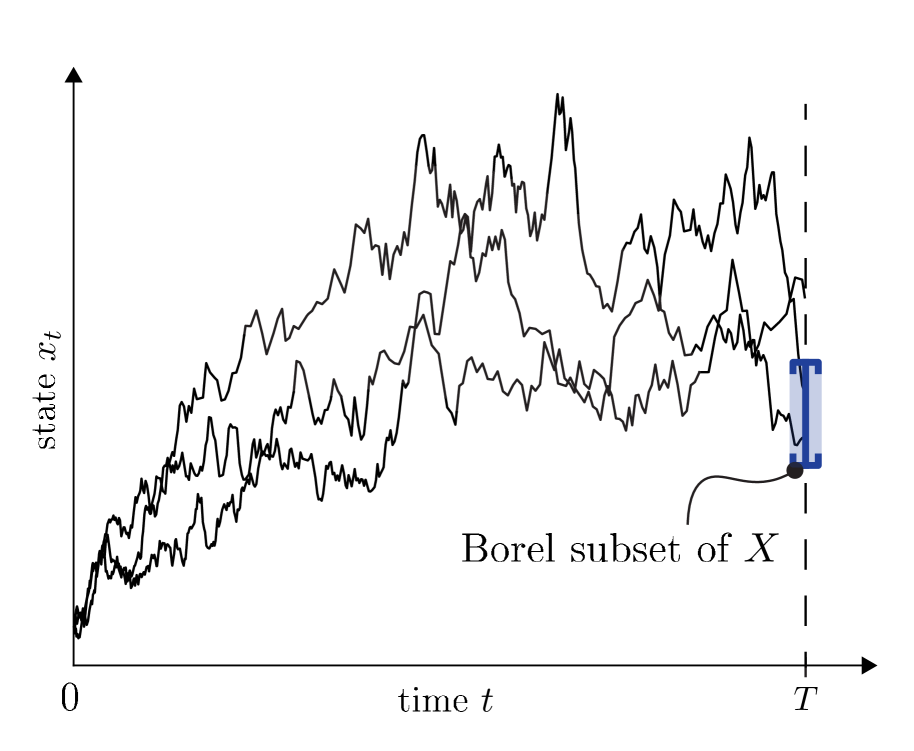
(a) The instantaneous occupation measure of the shaded set associated with the time $T$ is the probability to observe the process in the set at time $T$.

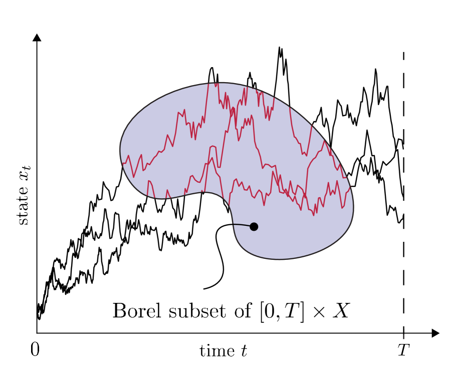
(b) The expected state occupation measure of the shaded set coincides with the expected length of the projection of the red portions of the process paths onto the $t$ axis.

Figure 1: Illustration of occupation measures

With these definitions, the expectations in Equation (1) can be expressed in terms of Lebesgue integrals with respect to $\nu_{0}$, $\nu_{t}$ and $\xi$:

$$\int_{X}w(t,x)\,d\nu_{t}(x)-\int_{X}w(0,x)\,d\nu_{0}(x)=\int_{[0,T]\times X\times U}\mathcal{A}w(s,x,u)\,d\xi(s,x,u).$$ (2)

Taking Observation 1 into account, Equation (2) shows that Dynkin’s formula not only describes an affine subspace of the occupation measures $\nu_{t}$ and $\xi$ but more importantly, under Assumption 1, also an affine subspace of their moments. We say that two measures $\nu_{t}$ and $\xi$ are a weak solution to (SDE) on the interval $[0,t]$ if the above relation is satisfied for all $w\in\mathcal{C}^{1,2}([0,t]\times X)$. This notion of weak solutions to (SDE) motivates the following weak form of (OCP):

$$\inf_{\nu_{T},\xi}\quad \int_{[0,T]\times X\times U}\ell(x,u)\,d\xi(t,x,u)+\int_{X}\phi(x)\,d\nu_{T}(x)$$ (weak OCP)

s.t. $$\int_{X}w(T,x)\,d\nu_{T}(x)-\int_{X}w(0,x)\,d\nu_{0}(x)=\int_{[0,T]\times X\times U}\mathcal{A}w(s,x,u)\,d\xi(s,x,u),$$

$$\hskip 227.62204pt\forall w\in\mathcal{C}^{1,2}([0,T]\times X),$$

$$\nu_{T}\in\mathcal{M}_{+}(X),$$

$$\xi\in\mathcal{M}_{+}([0,T]\times X\times U).$$

where $\mathcal{M}_{+}(Y)$ refers to the cone of finite, positive Borel measures supported on the set $Y$. While (weak OCP) remains intractable as an infinite dimensional linear program, Assumption 1 enables the construction of a sequence of increasingly tight SDP relaxations via the moment-sum-of-squares hierarchy [Par00, Las01]. This is achieved by relaxing (weak OCP) to optimization over the moments of the measures $\nu_{t}$ and $\xi$ up to finite order $d$ while imposing the affine constraints generated by Equation (2) and the necessary positive semidefinite constraints on the moment and localizing matrices reflecting non-negativity and support of both occupation measures; the relaxations can be tightened by increasing the maximum moment order $d$. The technical details for this construction are immaterial for our contribution so we instead refer the interested reader to [Las10].

The dual to (weak OCP) has an informative interpretation that serves as motivation for the discretization strategy presented in the next section. The dual reads

$$\sup_{w}\quad \int_{X}w(t,x)\,d\nu_{0}(x)$$ (subHJB)

s.t. $$\mathcal{A}w(t,x,u)+\ell(x,u)\geq 0,\quad\forall(t,x,u)\in[0,T]\times X\times U,$$ (3)

$$w(T,x)\leq\phi(x),\quad\forall x\in X,$$ (4)

$$w\in\mathcal{C}^{1,2}([0,T]\times X),$$

where the decision variable $w$ can be interpreted as a smooth underestimator of the value function associated with the control problem (OCP) [BB96].

Corollary 1.

Let $w$ be feasible for (subHJB). Then, $w$ underestimates the value function

$$V(t,z)=\inf_{u(\cdot)}\quad \mathbb{E}_{\delta_{z}}\left[\int_{t}^{T}\ell(x(s),u(s))\,ds+\phi(x(T))\right]$$ (5)

s.t. $$x(s)\text{ satisfies }\eqref{eq:SDE}\text{ on }[t,T]\text{ with }x(t)\sim\delta_{z},$$

$$x(s)\in X,$$

$$u(s)\in U.$$

on $[0,T]\times X$.

Proof.

Let $z\in X$ and $0\leq t\leq T$ and fix any admissible control policy $u$, i.e., a control policy such that any path of the stochastic process $(x(s),u(s))$ remains in $X\times U$ on $[t,T]$. Then, Constraints (3) and (4) imply that

$$\mathbb{E}_{\delta_{z}}\left[-\int_{t}^{T}\mathcal{A}w(s,x(s),u(s))\,ds+w(x(T))\right]\leq\mathbb{E}_{\delta_{z}}\left[\int_{t}^{T}\ell(x(s),u(s))\,ds+\phi(x(T))\right].$$

The left-hand-side coincides with $w(t,z)$ by Dynkin’s formula. Since the inequality holds for any admissible control policy, the result follows by minimizing the right-hand-side over all admissible control policies. ∎

Analogous to the primal counterpart, the moment-sum-of-squares hierarchy gives rise to a sequence of increasingly tight SDP restrictions of (subHJB) by restricting $w$ to be a polynomial of degree at most $d$ and imposing the non-negativity constraints by means of sufficient sum-of-squares conditions [Las01, Par00]. The resultant restrictions are loosened by increasing the degree $d$ of $w$.

In the following, we will use the dual perspective to devise a generalization of (subHJB) which, like its predecessor, enables computation of valid bounds for (OCP) via the moment-sum-of-squares hierarchy. From that, we will then construct the notion of local occupation measures.

3 The Dual Perspective revisited: Piecewise Polynomial Approximation

In order to construct better approximations to the value function in the spirit of (subHJB), we here propose to generalize problem (subHJB) by seeking a piecewise smooth underapproximation of the value function over the problem domain $[0,T]\times X$. To that end, we consider a discretization $0=t_{0}<t_{1}<\dots<t_{n_{T}}=T$ of the time domain and a partition $X_{1},X_{2},\dots,X_{n_{X}}$ of the state space $X$, i.e., $X=\cup_{k=1}^{n_{x}}X_{k}$ and $X_{i}\cap X_{j}=\emptyset$ if $i\neq j$. This allows us to form a partition of the whole problem domain as illustrated in Figure 2 and we can formulate the following natural generalization of (subHJB):

$$\sup_{w_{i,k}}\quad \sum_{k=1}^{n_{X}}\int_{X_{k}}w_{1,k}(0,x)\,d\nu_{0}(x)$$ (discretized subHJB)

s.t. $$\mathcal{A}w_{i,k}(t,x,u)+\ell(x,u)\geq 0,\quad\forall(t,x,u)\in[t_{i-1},t_{i}]\times X_{k}\times U,$$ (6)

$$w_{i,k}(t_{i-1},x)-w_{i-1,k}(t_{i-1},x)\geq 0,\quad\forall x\in X_{k},$$ (7)

$$w_{i,j}(t,x)-w_{i,k}(t,x)=0,\quad\forall(t,x)\in[t_{i-1},t_{i}]\times(\partial X_{j}\cap\partial X_{k}),$$ (8)

$$w_{n_{T},k}(T,x)\leq\phi(x),\quad\forall x\in X_{k},$$ (9)

$$w_{i,k}\in\mathcal{C}^{1,2}([0,T]\times X_{k}).$$ (10)

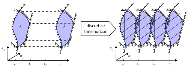
Figure 2: Discretization of space-time domain

The constraints in problem (discretized subHJB) are chosen to ensure that a valid underestimator of the value function can be constructed from the individual pieces $w_{i,k}$. This is formalized in the following Corollary.

Corollary 2.

Let $\{w_{i,k}:1\leq i\leq n_{T},1\leq k\leq n_{X}\}$ be feasible for (discretized subHJB) and define

$$w(t,x)=w_{i,k}(t,x)\text{ with }i=\sup\{j:t\in[t_{j-1},t_{j}]\}\text{ and }k\text{ such that }x\in X_{k}$$ (11)

Then, $w$ is an underestimator of the value function $V$ as defined in (5).

Proof Sketch.

The idea is to split the paths of the process $(t,x(t),u(t))$ up into pieces in which it is confined to a subdomain $[t_{i-1},t_{i}]\times X_{k}\times U$. For each of those pieces the same argument as in Corollary 1 applies to show that $w_{i,k}$ underestimates the value function on the respective subdomain. Additionally, Constraints (7) and (8) ensure conservatism when the process crosses between different time intervals and subdomains of the state space, respectively. Specifically, Constraint (7) enforces that $w(t,x(t))$ can at most increase when traced across the boundary between the intervals $[t_{i-1},t_{i}]$ and $[t_{i},t_{i+1}]$ ensuring that $w(t,z)$ cannot cross $V(t,z)$ at such time points. Likewise, Constraint (8) ensures that $w(t,z)$ cannot cross $V(t,z)$ when the process crosses between spatial subdomains by imposing the stronger continuity condition. The formal argument is presented in Appendix A. ∎

Remark 1.

Contrasting the monotonicity condition (7) enforced between subsequent time intervals, the stronger continuity requirement (8) at the boundary between subdomains of the state space is necessary as the process may cross the boundary in any direction due to stochastic vibrations. In case of a deterministic process ($g=0$) this condition may be further relaxed as we only require that $w(t,x(t))$ must at most increase for all trajectories of the system when crossing the boundary between two subdomains. [CKH21] show in a related argument that in this case it suffices to impose that

$$(w_{i,k}(t,x)-w_{i,j}(t,x))n_{j,k}^{\top}f(x,u)\geq 0,\quad\forall(t,x,u)\in[t_{i-1},t_{i}]\times(\partial X_{j}\cap\partial X_{k})\times U$$

where $n_{j,k}$ denotes the normal vector of the boundary between $X_{j}$ and $X_{k}$ pointing from $X_{j}$ to $X_{k}$.

Remark 2.

In the discussion of this section, we ignored that some elements of the partition $X_{1},\dots,X_{n_{X}}$ cannot be closed. We wish to emphasize, however, that this does not complicate the construction of valid moment-sum-of-squares restrictions of (discretized subHJB) as the non-negativity conditions can equivalently be enforced on the closure of the respective subdomains.

4 The Primal Perspective revisited: Local Occupation Measures

In this section, we briefly discuss the primal side of the construction presented in the previous section which gives rise to the localized notion of occupation measures. The primal corresponding to (discretized subHJB) reads

$$\inf_{\nu_{t_{i},k},\xi_{i,k},\pi_{i,j,k}}\quad \sum_{i=1}^{n_{T}}\sum_{k=1}^{n_{X}}\int_{[t_{i-1},t_{i}]\times X_{k}\times U}\ell(x,u)\,d\xi_{i,k}(t,x,u)+\sum_{k=1}^{n_{X}}\int_{X_{k}}\phi(T,x)\,d\nu_{t_{n_{T}},k}(x)$$ (discretized weak OCP)

s.t. $$\int_{X_{k}}w(t_{i},x)\,d\nu_{t_{i},k}(x)-\int_{X_{k}}w(t_{i-1},x)\,d\nu_{t_{i-1},k}(x)=$$

$$\hskip 28.45274pt\int_{[t_{i-1},t_{i}]\times X_{k}\times U}\mathcal{A}w(t,x,u)\,d\xi_{i,k}(t,x,u)+\sum_{\stackrel{{\scriptstyle j=1}}{{j\neq k}}}^{n_{X}}\int_{(t_{i-1},t_{i})\times(\partial X_{k}\cap\partial X_{j})}\,w(t,x)\,d\pi_{i,j,k}(t,x),$$

$$\hskip 256.0748pt\forall w\in\mathcal{C}^{1,2}([t_{i-1},t_{i}]\times X_{k}),$$

$$\nu_{t_{i},k}\in\mathcal{M}_{+}(X_{k}),$$

$$\xi_{i,k}\in\mathcal{M}_{+}([t_{i-1},t_{i}]\times X_{k}\times U),$$

$$\pi_{i,j,k}=-\pi_{i,k,j}\in\mathcal{M}((t_{i-1},t_{i})\times(\partial X_{j}\cap\partial X_{k}))$$

where $\mathcal{M}(Y)$ refers to the set of signed measures supported on $Y$. This problem reveals that discretization of the problem domain translates from this perspective into a “localized” notion of the occupation measures. Specifically, restriction of the expected state-action occupation measures $\xi$ introduced in Section 2 to a subdomain $[t_{i-1},t_{i}]\times X_{k}\times U$ from the partition (cf. Figure 3) yields the local state-action occupation measure $\xi_{i,k}$:

$$\xi_{i,k}(B_{T}\times B_{X}\times B_{U})=\xi((B_{T}\cap[t_{i-1},t_{i}])\times(B_{T}\cap X_{k})\times B_{U}).$$

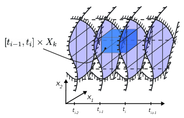
Figure 3: Support of local occupation measure $\xi_{i,k}$

Likewise, the local instantaneous occupation measures with respect to different time points $t_{i}$ and subdomains $X_{k}$ are given by the restriction of $\nu_{t_{i}}$ to $X_{k}$:

$$\nu_{t_{i},k}(B)=\nu_{t_{i}}(B\cap X_{k}).$$

The measures $\pi_{i,j,k}$ in the formulation of (discretized weak OCP) account for transitions of the process between the spatial subdomains $X_{j}$ to $X_{k}$ in the time interval $[t_{i-1},t_{i}]$. Formally, $\pi_{i,j,k}$ can be defined for any Borel subsets $B_{T}\subset(t_{i-1},t_{i})$ and $B_{\partial X}\subset\partial X_{j}\cap\partial X_{k}$ as

$$\pi_{i,j,k}(B_{T}\times B_{X})=\mathbb{E}_{\nu_{0}}\left[\sum_{n\in\mathbb{N}}(-1)^{n+1}\mathds{1}_{B_{T}}(\tau^{j}_{n})\mathds{1}_{B_{\partial X}}(x(\tau^{j}_{n}))\right]$$

where the $\tau^{j}_{n}$ denote the times at which the process enters and leaves the subdomain $X_{j}$, i.e.,

$$\tau^{j}_{n}=\begin{cases}t_{i-1},&n=0\\ \inf\left\{\tau^{j}_{n-1}<t<t_{i}:x(t)\in\begin{cases}X\setminus X_{j},&n\text{ odd}\\ X_{j},&n\text{ even}\end{cases}\right\},&n\geq 1\end{cases}.$$

Note that this definition indeed gives rise to a measure that satisfies the symmetry condition $\pi_{i,j,k}=-\pi_{i,k,j}$. Lastly, we wish to emphasize that it is easily verified that the relaxations derived from (discretized weak OCP) via the moment-sum-of-squares hierarchy are at least as tight as those derived from its traditional counterpart (weak OCP). To see this, note that the constraints in (weak OCP) are implied by the constraints in (discretized weak OCP) as $\xi=\sum_{k=1}^{n_{X}}\sum_{i=1}^{n_{T}}\xi_{i,k}$, $\sum_{k=1}^{n_{X}}\sum_{j=1,j\neq k}^{n_{X}}\pi_{i,j,k}=0$, and $\sum_{k=1}^{n_{X}}\nu_{t_{n_{T}},k}=\nu_{T}$.

5 Moment-Sum-of-Squares Approximations: Structure & Scalability

As already mentioned in Section 2, the construction of tractable relaxations of the problems (subHJB) or (weak OCP) relies on the restriction to optimization over polynomials or the relaxation to optimization over the finite sequence of moments up to some degree $d$, respectively. Traditionally, increasing this approximation order $d$ has been the only mechanism used to loosen the restriction, respectively strengthening the relaxation, to ultimately improve the obtained bounds to the desired level. The main motivation behind the proposed discretization approach lies in circumventing the combinatorial scaling associated with this tightening mechanism. With the proposed notion of local occupation measures, refinement of the domain discretization may be used as an additional bound tightening mechanism. Table 1 summarizes the scaling of the critical problem components of the moment-sum-of-squares SDP approximations of (discretized subHJB) and (weak OCP) with respect to the different tightening mechanisms of increasing $n_{X},n_{T}$ (refining the discretization) or $d$ (increasing the approximation order). The linear scaling of the SDP sizes with respect to $n_{X}$ and $n_{T}$ underlines the flexibility added by the proposed framework. While a naive refinement of the discretization will cause $n_{X}$ to scale itself combinatorially with the state space dimension, it opens the door to employ tailored refinement strategies with improved scaling and reap the computational rewards directly in the form of smaller SDPs. This finer control over the tightening process further enables exploitation of problem specific insights such as the knowledge of critical parts of the state space to be resolved more finely than others to construct tighter relaxations. This flexibility is in stark contrast to increasing the approximation order $d$ as translating such insights into specific moments to be constrained or monomial terms to be considered in the value function approximator is significantly less straightforward as highlighted by several works on sparse moment-sum-of-squares hierarchies [SK20, Wan+21, ZFP19]. In this context, it is further worth emphasizing that not only the linear scaling with respect to $n_{T}$ and $n_{X}$ is desirable but in particular the invariance of the linear matrix inequality (LMI) dimension promotes scalability [AM14, ADH17, AH19, AM19].

	#variables	# LMIs	dimension of LMIs
$d$	$O({n+d\choose d})$	$O(1)$	$O({n+\left\lfloor d/2\right\rfloor\choose\left\lfloor d/2\right\rfloor})$
$n_{T}$	$O(n_{T})$	$O(n_{T})$	$O(1)$
$n_{X}$	$O(n_{X})$	$O(n_{X})$	$O(1)$

Table 1: Scaling of moment-sum-of-squares SDP approximations with respect to different tightening mechanisms

Aside from the favorable scaling properties, the problems (discretized subHJB) and (weak OCP) give rise to highly structured SDPs. Specifically, all constraints involve only variables corresponding to adjacent subdomains ($\partial X_{j}\cap\partial X_{k}\neq\emptyset$). As a consequence, the structure of the constraints is analogous to those arising from discretized PDEs which could potentially be exploited in tailored, distributed optimization algorithms.

6 Case Study: Population Control

6.1 Control Problem

We study the proposed local occupation measure framework and its computational implications with an example problem from the field of population control. The problem is adjusted from [SLD09] where it has been studied in a discrete time, infinite horizon setting. The objective is to control the population size of a primary predator and its prey in an ecosystem featuring the prey species, primary predator species as well as a secondary predator species with an erratically changing population size. The interactions between the primary predator and prey population are assumed to be described by a standard Lotka-Volterra model, while the effect of presence/absence of the secondary predator species is modeled by a Brownian motion. The population sizes are assumed to be controlled via hunting of the primary predator species. This model gives rise to the diffusion process,

$$dx(t)=\begin{bmatrix}\gamma_{1}x_{1}(t)-\gamma_{2}x_{1}(t)x_{2}(t)\\ \gamma_{4}x_{1}(t)x_{2}(t)-\gamma_{3}x_{2}(t)-x_{2}(t)u(t)\end{bmatrix}\,dt+\begin{bmatrix}\gamma_{5}x_{1}(t)\\ 0\end{bmatrix}\,db(t),$$

where $x_{1}$, $x_{2}$, and $u$ refer to the prey species, predator species and hunting effort, respectively. The model parameters $\gamma=(1,2,1,2,0.025)$ and initial condition $x(0)\sim\delta_{(1,0.25)}$ are assumed to be known deterministically. Moreover, we assume that the admissible hunting effort is confined to $U=[0,1]$. Under these assumptions, it is easily verified that the process $x(t)$ is by construction confined to the non-negative orthant $X=\{x:x_{1},x_{2}\geq 0\}$ for any admissible control policy. For the control problem we further choose a time horizon of $T=10$ and stage cost

$$\ell(x,u)=(x_{1}-0.75)^{2}+\frac{(x_{2}-0.5)^{2}}{10}+\frac{(u-0.5)^{2}}{10}$$

penalizing variations from the target population sizes.

6.2 Discretization of Problem Domain

In order to investigate the effect of different discretizations on bound quality and computational cost, we utilize a simple grid partition of the state space $X$ as parameterized by the number of grid cells $n_{1}$ and $n_{2}$ in the $x_{1}$ and $x_{2}$ direction, respectively. As $X$ is the non-negative orthant in our example, and hence semi-infinite, we choose to discretize the compact interval box $[0,1.5]\times[0,1.5]$ with a uniform grid of $(n_{1}-1)\times(n_{2}-1)$ cells and cover the remainder of $X$ with appropriately chosen semi-infinite interval boxes. This choice is motivated by the fact that the uncontrolled system resides with high probability in this part of the state space. The resultant grid is illustrated in Figure 4. Note further that any cell of the described grid is by construction a basic closed semialgebraic set. As a consequence, sufficient sum-of-squares conditions for non-negativity of a polynomial on such a grid cell are provided by standard sum-of-squares arguments.

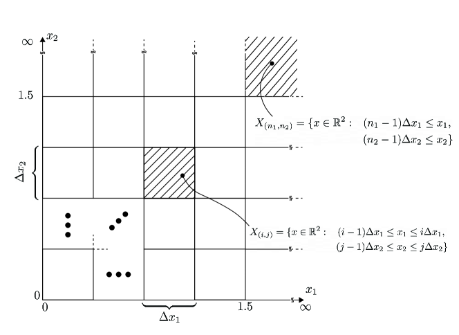
Figure 4: Spatial discretization of $X=\mathbb{R}^{n}_{+}$ using $n_{1}\times n_{2}$ interval boxes. The spatial discretization is chosen as uniform on $[0,1.5]\times[0,1.5]$.

The temporal domain is discretized uniformly into $n_{T}$ subintervals, i.e., $t_{i}=i\Delta t$ with $\Delta t=\frac{T}{n_{T}-1}$. Throughout we will only refer to a specific discretization with the associated triple $(n_{1},n_{2},n_{T})$. The computational experiments are conducted for all discretizations corresponding to the triples $\{(n_{1},n_{2},n_{T}):1\leq n_{1},n_{2}\leq 5,1\leq n_{T}\leq 10\}$.

6.3 Evaluation of Bound Quality

In order to assess the tightness of the bounds obtained with different approximation orders and discretizations, we compare the relative optimality gap defined as

$$\text{rel. optimality gap }=\frac{UB-LB}{UB}$$

where $LB$ refers to the lower bound furnished by a concrete instance of the moment-sum-of-squares restriction of (discretized subHJB), and $UB$ to the control cost associated with the best known admissible control policy. In order to determine $UB$, we constructed an admissible control policy from the approximate value function $w^{*}$ obtained as solution of the moment-sum-of-squares restriction of (discretized subHJB) with approximation order $d=4$ on the grid described by $n_{1}=n_{2}=4$ and $n_{T}=10$. Specifically, we employed the following control law mimicking a one-step model-predictive controller

$$u^{*}(t)\in\operatorname*{arg\,min}_{u\in dU}\mathcal{A}w^{*}(t,x(t),u)+\ell(x(t),u)$$

where $dU=\{0,0.05,0.1,\dots,1\}\subset U$. The best known control cost

$$UB=\mathbb{E}_{\nu_{0}}\left[\int_{[0,\infty)}\ell(x(t),u^{*}(t))\,dt\right]$$

was then estimated by the ensemble average of $10,000$ sample trajectories. A comparison of the sample trajectories for the controlled and uncontrolled process is shown in Figure 5.

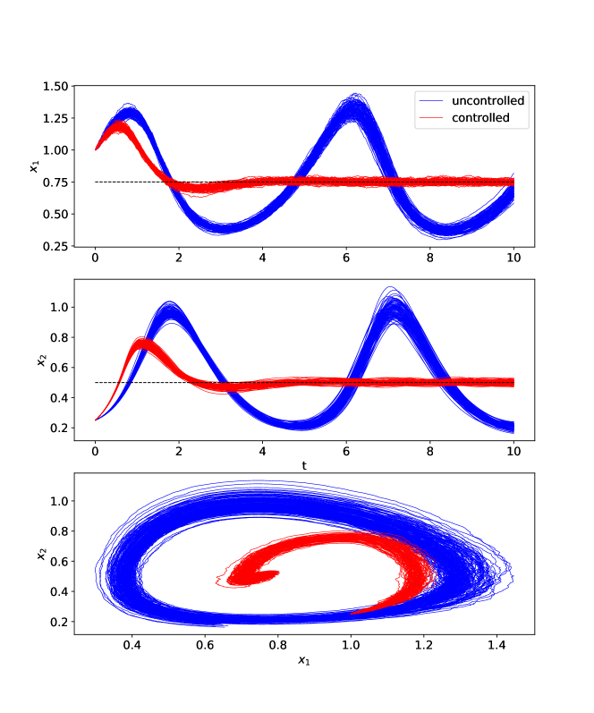
Figure 5: Comparison between uncontrolled system and system controlled via best-known control policy $u^{*}$

6.4 Computational Details

All computational experiments presented in this section were conducted on a MacBook Pro with Apple M1 Pro with 16GB unified memory. All sum-of-squares programs and the associated SDPs were constructed using the custom developed package MarkovBounds.jl built on top of SumOfSquares.jl [Wei+19] and solved with Mosek v9.0.87.

6.5 Results

We put special emphasis on investigating the effect of refining the discretization of the problem domain on bound quality and computational cost. Focusing on the effect on computational cost in isolation first, Figure 6 indicates that the computational cost for the solution of moment-sum-of-squares programs generated by the restriction of (discretized subHJB) to polynomials of degree at most $d$ scales approximately linearly with the number of cells $n_{1}\times n_{2}\times n_{T}$ of the spatiotemporal partition. On the other hand, Figure 6 also shows that increasing the approximation order $d$ results in a much more rapid increase in computational cost. These results are perfectly in line with the discussion in Section 5.

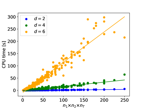
Figure 6: Computational cost scales approximately linearly with number of grid cells for fixed approximation order

Figure 7 further shows the trade-off between bound quality and the associated computational cost for different approximation orders and discretization grids. First, it is worth noting that the proposed discretization strategy enables the computation of overall tighter bounds with an approximation order of only up to $d=6$ when compared to the traditional formulation with an approximation order of up to $d=14$. It is further worth emphasizing that beyond $d=14$, numerical issues prohibited an accurate solution of the SDPs arising from the traditional formulation such that no tighter bounds could be obtained this way. Furthermore, the figure also indicates that across almost the entire accuracy range, a significant speed up ($>5\times$) can be achieved by using the proposed discretization strategy instead of only increasing the approximation order as done traditionally. Lastly, the results clearly show that a careful choice of discretization is crucial to achieve good performance. Figure 7(b) indicates that for this example particularly good performance is achieved when only the time domain is discretized; additionally discretizing the spatial domain becomes an effective means of bound tightening only after the time domain has already been resolved sufficiently finely.

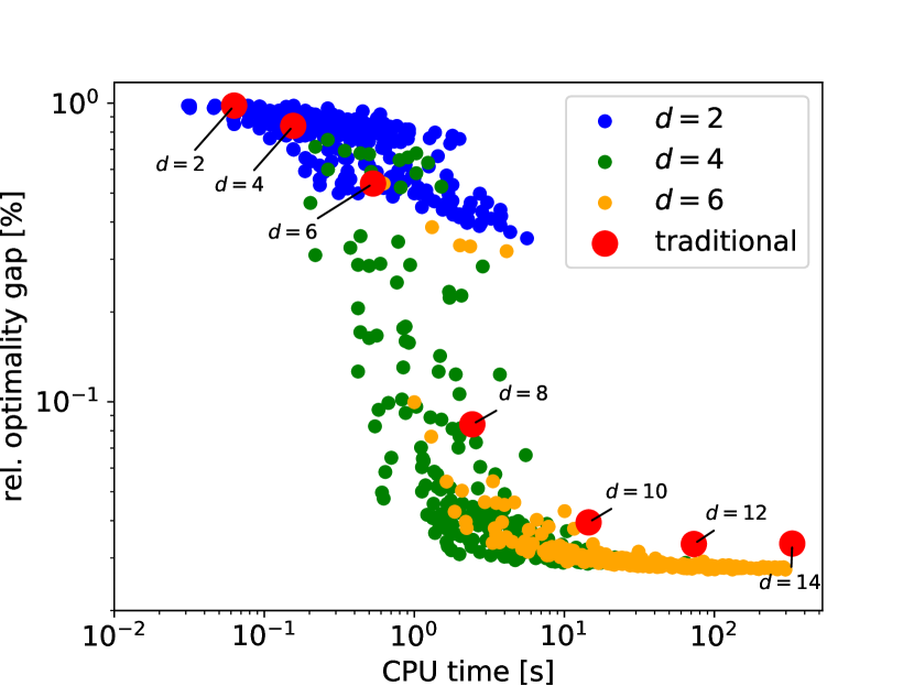
(a) spatial & temporal discretization

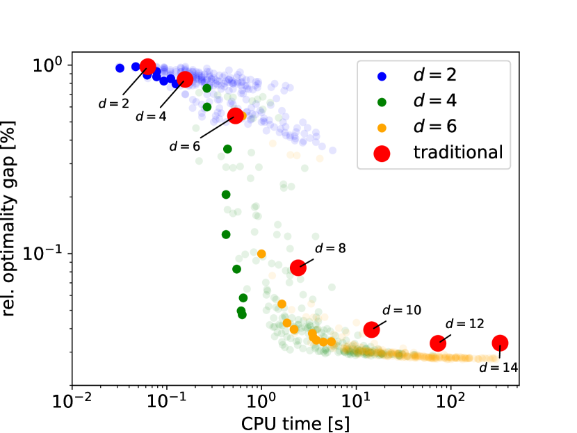
(b) temporal discretization highlighted ($n_{1}=n_{2}=1$)

Figure 7: Trade-off between computational cost and bound quality for different approximation orders $d$ and domain discretizations $(n_{1},n_{2},n_{T})$. The red markers correspond to moment-sum-of-squares restrictions of the labeled approximation order for the traditional formulation (subHJB) without any discretization.

7 Extensions

Before we close, we briefly showcase two direct extensions to the described local occupation measure framework showcasing its versatility.

7.1 Discounted Infinite Horizon Problems

Consider the following discounted infinite horizon stochastic control problem with discount factor $\rho>0$:

$$\inf_{u(\cdot)}\quad \mathbb{E}_{\nu_{0}}\left[\int_{[0,\infty)}e^{-\rho t}\ell(x(t),u(t))\,dt\right]$$

s.t. $$x(t)\text{ satisfies \eqref{eq:SDE} on }[0,\infty)$$

$$x(t)\in X$$

$$u(t)\in U.$$

The construction of a weak formulation of this problem akin (weak OCP) can be done in full analogy to Section 2. To that end, note that the infinitesimal generator $\mathcal{A}$ maps functions of the form $\hat{w}(t,x)=e^{-\rho t}w(t,x)$ to functions of the same form, i.e.,

$$\mathcal{A}\hat{w}(t,x,u)=e^{-\rho t}(\mathcal{A}w(t,x,u)-\rho w(t,x,u)).$$

By analogous arguments as in Section 2, it therefore follows that any function $w\in C^{1,2}([0,\infty)\times X)$ that satisfies

$$\mathcal{A}w(t,x,u)-\rho w(t,x,u)+\ell(x,u)\geq 0,\quad\forall(t,x,u)\in[0,\infty)\times X\times U$$

furnishes a valid subsolution $\hat{w}(t,x)=e^{-\rho t}w(t,x)$ of the value function associated with the infinite horizon problem. Since the proposed discretization approach does neither rely on boundedness of the state space nor control horizon in order to establish valid bounds, it follows that it readily extends to the infinite horizon setting. Moreover, additional assumptions or insights on the structure of the value function can be easily incorporated via appropriate constraints. One example for such additional insights could be the invariance of the value function with respect to time, which is well-known for many infinite horizon control problems [OS07].

7.2 Jump Processes with Discrete State Space

Many fields and applications ranging from chemical physics to queuing theory call for models that describe stochastic transitions between discrete states. In those cases, jump processes are a common modeling choice [Gil92, Bre03]. In the following, we will show that the proposed local occupation measure framework extends with only minor modifications to stochastic optimal control of a large class of such jump processes. Specifically, we will consider controlled, continuous-time jump processes driven by $m$ independent Poisson counters $n_{i}(t)$ with associated propensities $a_{i}(x(t),u(t))$:

$$dx(t)=\sum_{i=1}^{m}h_{i}(x(t),u(t))-x(t)\,dn_{i}(t).$$ (JDE)

We will again assume that the process can be fully characterized by polynomials, but we now additionally impose the assumption that the state space of the process is discrete.

Assumption 2.

The jumps $h_{i}:X\times U\to X$, propensities $a_{i}:X\times U\to\mathbb{R}_{+}$, stage cost $l:X\times U\to\mathbb{R}$ and terminal cost $\phi:X\times U\to\mathbb{R}$ are polynomial functions jointly in both arguments. The state space is a discrete, countable set and the set of admissible control inputs $U$ is a basic semialgebraic.

The local occupation measure framework outlined previously for diffusion processes can be effectively extended for computing lower bounds on stochastic optimal control problems with such jump processes embedded. Specifically, we consider stochastic optimal control problems of the form

$$\inf_{u(\cdot)}\quad \mathbb{E}_{\nu_{0}}\left[\int_{[0,T]}\ell(x(t),u(t))\,dt+\phi(x(T))\right]$$ (jump OCP)

s.t. $$x(t)\text{ satisfies \eqref{eq:JDE} on }[0,T]\text{ with }x(0)\sim\nu_{0},$$

$$x(t)\in X,$$

$$u(t)\in U$$

where $\ell:X\times U\to\mathbb{R}$ and $\phi:X\to\mathbb{R}$ are again polynomials. The extended infinitesimal generator $\mathcal{A}:\mathcal{C}^{1,0}([0,T]\times X)\to\mathcal{C}([0,T]\times X\times U)$ of a process described by (JDE) is given by

$$\mathcal{A}w\mapsto\frac{\partial w}{\partial t}(t,x)+\sum_{i=1}^{m}a_{i}(x,u)\left(w(t,h_{i}(x,u))-w(t,x)\right).$$

Note that under Assumption 2, $\mathcal{A}$ again maps polynomials to polynomials providing the basis for application of the moment-sum-of-squares hierarchy for construction of tractable relaxations of (jump OCP). The weak form of (jump OCP) and its dual take a form essentially identical to (weak OCP) and (subHJB) where (subHJB) again can be tied to seeking the maximal subsolution to the value function associated with (jump OCP). For the sake brevity, we discuss these details in Appendix B. Unlike in Section 2, however, $X$ is now only closed basic semialgebraic if and only if it is finite. Thus, the moment-sum-of-squares hierarchy provides finite SDP relaxations of the weak form counterpart of (jump OCP) only in the case of a finite state space $X$. Moreover, these relaxations may in fact not even be practically tractable if $X$ is finite but has a large cardinality. If $X$ is infinite (or of very large cardinality), tractable moment-sum-of-squares relaxations can only be constructed at the price of introducing additional conservatism. From the primal perspective, this additional conservatism is introduced by optimizing over measures supported on a basic closed semialgebraic overapproximation of $X$ in (weak OCP). This overapproximation is usually chosen to be a polyhedral or box superset of $X$ due to simple computational treatment [DB18, Dow19]. The framework of local occupation measures provides a way to reduce the conservatism introduced by such a basic closed semialgebraic overapproximation of $X$, in particular in the case of polyhedral overapproximations. To appreciate this fact, consider a partition $X_{1},\dots,X_{n_{X}}$ of the state space $X$ and a discretization $t_{0}<t_{1}<\dots<t_{n_{T}}=T$ of the control horizon. Given such a partition, the dual of the weak form stochastic optimal control problem takes the form

$$\sup_{w_{i,k}}\quad \sum_{k=1}^{n_{X}}\int_{X_{k}}w_{1,k}(0,x)\,d\nu_{0}(x)$$ (jump discHJB)

s.t. $$\mathcal{A}w_{i,k}(t,x,u)+\ell(x,u)\geq 0,\quad\forall(t,x,u)\in[t_{i-1},t_{i}]\times X_{k}\times U,$$

$$w_{i,k}(t_{i-1},x)-w_{i-1,k}(t_{i-1},x)\geq 0,\quad\forall x\in X_{k},$$

$$w_{i,j}(t,x)-w_{i,k}(t,x)=0,\quad\forall(t,x)\in[t_{i-1},t_{i}]\times N_{X_{k}}(X_{j}),$$

$$w_{n_{T},k}(T,x)\leq\phi(x),\quad\forall x\in X_{k}$$

where $N_{X_{k}}(X_{j})$ denotes the “neighborhood” of $X_{k}$ in $X_{j}$ defined as all states in $X_{j}$ which have a non-zero transition probability into $X_{k}$; formally,

$$N_{X_{k}}(X_{j})=\{x\in X_{j}:\exists u\in U\text{ s.t. }h_{i}(x,u)\in X_{k}\text{ for some }i\text{ and }a_{i}(x,u)>0\}.$$

In order to construct tractable relaxations for the above problem via the moment-sum-of-squares hierarchy, it of course remains still necessary to replace any infinite (or very large) partition element by a closed basic semialgebraic overapproximation; however, as Figure 8 illustrates, the union of overapproximations of the individual subdomains will generally be less conservative than an overapproximation chosen for the whole state space.

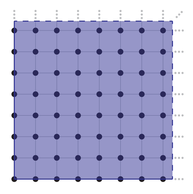
(a)

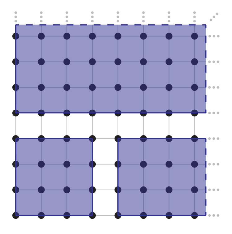
(b)

Figure 8: Overapproximation of a semi-infinite lattice by a box (a) vs. overapproximation by the union of box-overapproximations of a three-element partition of the same semi-infinite lattice (b).

7.3 Example: Optimal gene regulation for protein expression

In order to demonstrate the effectiveness of the proposed local occupation measure framework for the optimal control of jump processes, we consider here the problem of protein regulation in a cell. We assume that the protein expression is biologically implemented via a simple biocircuit as shown in Figure 9.

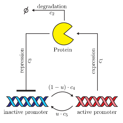
Figure 9: Simplified biocircuit model for gene regulation

The biocircuit is modeled as a jump process reflecting the stochastic nature of chemical reactions in cellular environments due to low molecular copy numbers [Gil92]. The resultant jump process has three states encoding the molecular counts of protein $x_{1}$, active promoter $x_{2}$ and inactive promoter $x_{3}$. The expression of protein can be controlled indirectly via the activation kinetics of the promoter. The resultant jump process is summarized by the following transitions with associated rates:

$$h_{1}:(x_{1},x_{2},x_{3})\mapsto(x_{1}+1,x_{2},x_{3}),\quad a_{1}(x,u)=10x_{2}$$ (expression)

$$h_{2}:(x_{1},x_{2},x_{3})\mapsto(x_{1}-1,x_{2},x_{3}),\quad a_{2}(x,u)=0.1x_{1}$$ (degradation)

$$h_{3}:(x_{1},x_{2},x_{3})\mapsto(x_{1},x_{2}-1,x_{3}+1),\quad a_{3}(x,u)=0.1x_{1}x_{2}$$ (repression)

$$h_{4}:(x_{1},x_{2},x_{3})\mapsto(x_{1},x_{2}+1,x_{3}-1),\quad a_{4}(x,u)=10(1-u)x_{3}$$ (activation)

$$h_{5}:(x_{1},x_{2},x_{3})\mapsto(x_{1},x_{2}-1,x_{3}+1),\quad a_{5}(x,u)=10ux_{2}$$ (inactivation)

Admissible control actions $u$ are constrained to lie within the interval $U=[0,1]$. Moreover, we assume a deterministic initial condition $x(0)\sim\delta_{(0,1,0)}$ and exploit that due to the reaction invariant $x_{2}(t)+x_{3}(t)=x_{2}(0)+x_{3}(0)$ the state space $X$ is effectively two-dimensional, i.e., we eliminate $x_{3}(t)=1-x_{2}(t)$. It can be easily verified that, after elimination of the reaction invariant, the state space of the jump process is given by

$$X=\{x\in\mathbb{Z}_{+}^{2}:x_{2}\in\{0,1\}\}$$

such that Assumption 2 is satisfied. The goal of the control problem is to stabilize the protein level in the cell at a desired value of 10 molecules. To that end, we choose to minimize the stage cost

$$\ell(x,u)=(x_{1}(t)-10)^{2}+10(u-0.5)^{2}$$

over the horizon $[0,10]$.

In order to investigate the effect of different discretizations of the problem domain on bound quality and computational cost, we discretize the time horizon uniformly into $n_{T}$ intervals and partition the state space into the singletons

$$X_{i}=\begin{cases}\{(i-1,0),&i\leq n_{X}\\ \{(i-n_{X}-1,1)\},&i>n_{X}\end{cases}\text{ for }i=1,\dots,2n_{X}$$

and capture the remaining part of the state space in the last partition element

$$X_{2n_{X}+1}=\{x\in\mathbb{Z}_{+}^{2}:x_{1}\geq n_{X},x_{2}\in\{0,1\}\}.$$

By changing the parameters $n_{T}$ and $n_{X}$, the fineness of the partition of the problem domain can be modulated. For this example, we explore parameter values in the ranges $n_{T}\in\{2,4,\dots,8,20\}$ and $n_{X}\in\{0,8,\dots,32,40\}$.

Note that the partition elements $X_{1},\dots,X_{2n_{X}}$ are already basic closed semialgebraic such that no overapproximation is required for the construction of valid moment-sum-of-squares restriction of the non-negativity constraints in (jump discHJB). In contrast, $X_{2n_{X}+1}$ is infinite, hence not basic closed semialgebraic. We therefore strengthen the formulation of the moment-sum-of-squares restriction of (jump discHJB) by imposing the non-negativity conditions on the convex hull of $X_{2n_{X}+1}$, thereby recovering tractability.

In order to estimate the bound quality we follow a strategy analogous to that described in Section 6.3.

Figure 10 shows a comparison of the trade-off between computational cost and bound quality achieved by different choices for the partition of the problem domain and approximation order. The results obtained with the classical occupation measure framework are emphasized with enlarged red markers. As already found for the example considered in Section 6, the results show that by adequately partitioning the problem domain the computational cost to compute bounds of a given quality can be substantially reduced compared to the traditional approach. In fact, it is again observed that tighter bounds could be computed in significantly less time than with the traditional approach.

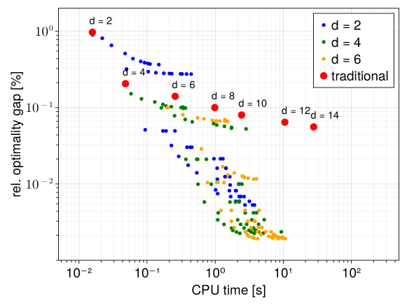
Figure 10: Trade-off between computational cost and bound quality for different approximation orders $d$ and domain partitions (different markers).

8 Conclusion

We have proposed and investigated a simple discretization strategy akin that used for the numerical solution of PDEs in order to improve the scalability of moment-sum-of-squares relaxations for stochastic optimal control problems. From the dual perspective this strategy can be interpreted as finding the tightest piecewise polynomial underestimator of the value function. Our analysis further revealed that the primal perspective motivates a localized notion of occupation measures obtained by restricting the traditional notion occupation measures to subdomains of a partition of the state space and control horizon. The key advantage of the proposed framework is that it offers a flexible way to tighten the SDP relaxations at linearly increasing cost, simply by refining the partition. This is in stark contrast to the traditional tightening mechanism of increasing the approximation order which results in combinatorial scaling. Two examples illustrate that the proposed strategy can indeed improve the efficiency and practicality of the occupation measure approach to stochastic optimal control by a moderate amount.

For future work, we seek to investigate if and how the use of distributed optimization techniques can further improve efficiency of the proposed framework by exploiting the weakly-coupled block structure of the SDP relaxations.

Appendix A Proof of Corollary 1

Proof.

Fix $z\in X$. Now consider an admissible control policy $u$ such that all paths of the control process $(x(s),u(s))\in X\times U$ $\forall s\in[t,T]$ with $x(t)\sim\delta_{z}\in X$ and $t\in[t_{n_{T}-1},T]$ are feasible. Further define $\tau_{0}=t$ and $\tau_{i}$ for $i\geq 1$ to be the minimum between $T$ and the time point at which the process crosses for the $i$^th time from one subdomain of the partition $X_{1},\dots,X_{n_{X}}$ to another. By definition, the process is confined to some (random) subdomain $X_{k}$ in the interval $[\tau_{i},\tau_{i+1}]$. Since $w_{n_{T},k}$ is sufficiently smooth on $[\tau_{i},\tau_{i+1}]\times X_{k}$, Ito’s lemma applies and yields that

$$w_{n_{T},k}(\tau_{i+1},x(\tau_{i+1}))=w_{n_{T},k}(\tau_{i},x(\tau_{i}))+\int_{\tau_{i}}^{\tau_{i+1}}\mathcal{A}w_{n_{T},k}(s,x(s),u(s))\,ds\\ +\int_{\tau_{i}}^{\tau_{i+1}}\nabla_{x}w_{n_{T},k}(s,x(s))^{\top}g(x(s),u(s))\,db(s).$$

Now note that by Constraint (6),

$$\int_{\tau_{i}}^{\tau_{i+1}}\mathcal{A}w_{n_{T},k}(s,x(s),u(s))\,ds\geq-\int_{\tau_{i}}^{\tau_{i+1}}\ell(x(s),u(s))\,ds.$$

Further note that

$$\mathbb{E}_{\delta_{z}}\left[\int_{\tau_{i}}^{\tau_{i+1}}\nabla_{x}w_{n_{T},k}(s,x(s))^{\top}g(x(s),u(s))\,db(s)\right]=0$$

as the integrand is square-integrable by Assumption 1 and $\tau_{i}\leq\tau_{i+1}$ are stopping times with respect to the natural filtration (see [IW14], Chapter 2, Proposition 1.1). Thus, after taking expectations, we obtain

$$\mathbb{E}_{\delta_{z}}\left[w_{n_{T},k}(\tau_{i},x(\tau_{i}))\right]\leq\mathbb{E}_{\delta_{z}}\left[\int_{\tau_{i}}^{\tau_{i+1}}\ell(x(s),u(s))\,ds+w_{n_{T},k}(\tau_{i+1},x(\tau_{i+1}))\right].$$

Moreover, continuity holds at any crossings between subdomains $X_{k}$ and $X_{j}$ due to Constraint (8) such that

$$\mathbb{E}_{\delta_{z}}\left[w(\tau_{i},x(\tau_{i}))\right]=\mathbb{E}_{\delta_{z}}\left[w_{n_{T},k}(\tau_{i},x(\tau_{i}))\right]=\mathbb{E}_{\delta_{z}}\left[w_{n_{T},j}(\tau_{i},x(\tau_{i}))\right]$$

when the process crosses from $X_{k}$ to $X_{j}$ at $\tau_{i}$. Now using that $\mathbb{E}_{\delta_{z}}\left[w(\tau_{0},x(\tau_{0}))\right]=w(t,z)$, we obtain by summing over the time intervals $[\tau_{0},\tau_{1}],\dots,[\tau_{N},\tau_{N+1}]$ that

$$w(t,z)\leq\mathbb{E}_{\delta_{z}}\left[\sum_{i=0}^{N}\int_{\tau_{i}}^{\tau_{i+1}}\ell(x(s),u(s))\,ds+w(\tau_{N+1},x(\tau_{N+1}))\,ds\right]=\mathbb{E}_{\delta_{z}}\left[\int_{t}^{\tau_{i+1}}\ell(x(s),u(s))\,dt+w(\tau_{N+1},x(\tau_{N+1}))\,ds\right].$$

Letting $N\to\infty$, it follows that

$$w(t,z)\leq\mathbb{E}_{\delta_{z}}\left[\int_{t}^{T}\ell(x(s),u(s))\,ds+w(T,x(T))\right]$$

as $\tau_{N}\to T$ (almost) surly. Finally using that $w(T,x)\leq\phi(x)$ on $X$ due to Constraint (9) and the fact that all results hold for any admissible control policy, we obtain the desired result $w(t,z)\leq V(t,z)$.

It remains to show that $w$ preserves the lower bounding property across the boundaries introduced by discretization of the time domain. To that end, note that by an analogous argument as before, we have for any $t\in[t_{i-1},t_{i})$ that

$$w(t,z)\leq\mathbb{E}_{\delta_{z}}\left[\int_{t}^{t_{i}}\ell(x(s),u(s))\,dt+\lim_{s\nearrow t_{i}}w(s,x(t_{i}))\right].$$

Since Constraint (7) implies that $\lim_{s\nearrow t_{i}}w(s,x)\leq w(t_{i},x)$ on $X$, it finally follows by induction that $w(t,z)\leq V(t,z)$ for any $t\in[0,T]$ and $z\in X$. ∎

Appendix B Weak form stochastic optimal control with embedded jump process on a discrete state space

The weak form of stochastic optimal control of a jump process on a discrete state space is given by

$$\inf_{\nu_{T},\xi}\quad \int_{[0,T]\times X\times U}\ell(x,u)\,d\xi(t,x,u)+\int_{X}\phi(x)\,d\nu_{T}(x)$$

s.t. $$\int_{X}w(T,x)\,d\nu_{T}(x)-\int_{X}w(0,x)\,d\nu_{0}(x)=\int_{[0,T]\times X\times U}\mathcal{A}w(s,x,u)\,d\xi(s,x,u),$$

$$\hskip 227.62204pt\forall w\in\mathcal{C}^{1,2}([0,T]\times X),$$

$$\nu_{T}\in\mathcal{M}_{+}(X),$$

$$\xi\in\mathcal{M}_{+}([0,T]\times X\times U).$$

where the occupation measures $\nu_{T}$ and $\xi$ are defined as in Section 2. The corresponding dual is given by

$$\sup_{w}\quad \int_{X}w(t,x)\,d\nu_{0}(x)$$

s.t. $$\mathcal{A}w(t,x,u)+\ell(x,u)\geq 0,\quad\forall(t,x,u)\in[0,T]\times X\times U,$$

$$w(T,x)\leq\phi(x),\quad\forall x\in X,$$

$$w\in\mathcal{C}^{1,0}([0,T]\times X),$$

and characterizes again the maximal smooth subsolution of the value function associated with (jump OCP).

References

- [ADH17] Amir Ali Ahmadi, Sanjeeb Dash and Georgina Hall “Optimization over structured subsets of positive semidefinite matrices via column generation” In Discrete Optimization 24 Elsevier, 2017, pp. 129–151
- [AH19] Amir Ali Ahmadi and Georgina Hall “On the construction of converging hierarchies for polynomial optimization based on certificates of global positivity” In Mathematics of Operations Research 44.4 INFORMS, 2019, pp. 1192–1207
- [AM14] Amir Ali Ahmadi and Anirudha Majumdar “DSOS and SDSOS optimization: LP and SOCP-based alternatives to sum of squares optimization” In 2014 48th Annual Conference on Information Sciences and Systems (CISS), 2014, pp. 1–5 IEEE
- [AM19] Amir Ali Ahmadi and Anirudha Majumdar “DSOS and SDSOS optimization: more tractable alternatives to sum of squares and semidefinite optimization” In SIAM Journal on Applied Algebra and Geometry 3.2 SIAM, 2019, pp. 193–230
- [BB96] Abhay G. Bhatt and Vivek S. Borkar “Occupation Measures for Controlled Markov Processes: Characterization and Optimality” In The Annals of Probability 24.3, 1996, pp. 1531–1562
- [Boy+10] Stephen Boyd, Neal Parikh, Eric Chu, Borja Peleato and Jonathan Eckstein “Distributed optimization and statistical learning via the alternating direction method of multipliers” In Foundations and Trends in Machine Learning 3.1, 2010, pp. 1–122 DOI: 10.1561/2200000016
- [Bre03] Lothar Breuer “From Markov jump processes to spatial queues” Springer Science & Business Media, 2003
- [CKH21] Vit Cibulka, Milan Korda and Tomáš Haniš “Spatio-temporal decomposition of sum-of-squares programs for the region of attraction and reachability” In IEEE Control Systems Letters 6 IEEE, 2021, pp. 812–817
- [DB18] Garrett R Dowdy and Paul I Barton “Bounds on stochastic chemical kinetic systems at steady state” In The Journal of Chemical Physics 148.8 AIP Publishing, 2018, pp. 84106
- [Dow19] Garrett Ryan Dowdy “Using semidefinite programming to bound distributions in chemical engineering systems”, 2019
- [FV89] Wendell H. Fleming and Domokos Vermes “Convex duality approach to the optimal control of diffusions” In SIAM Journal on Control and Optimization 27.5, 1989, pp. 1136–1155 DOI: 10.1137/0327060
- [Gil92] Daniel T Gillespie “A rigorous derivation of the chemical master equation” In Physica A: Statistical Mechanics and its Applications 188.1-3 Elsevier, 1992, pp. 404–425
- [HRS01] Kurt Helmes, Stefan Röhl and Richard H Stockbridge “Computing Moments of the Exit Time Distribution for Markov Processes by Linear Programming” In Operations Research 49.4 INFORMS, 2001, pp. 516–530
- [HB21] Flemming Holtorf and Paul I Barton “Tighter bounds on transient moments of stochastic chemical systems”, 2021
- [IW14] Nobuyuki Ikeda and Shinzo Watanabe “Stochastic Differential Equations and Diffusion Processes” Elsevier, 2014 DOI: 10.2307/1268562
- [KS98] Thomas G. Kurtz and Richard H. Stockbridge “Existence of Markov Controls and Characterization of Optimal Markov Controls” In SIAM Journal on Control and Optimization 36.2, 1998, pp. 609–653 DOI: 10.1137/S0363012995295516
- [Las01] Jean B Lasserre “Global optimization with polynomials and the problem of moments” In SIAM Journal on Optimization 11.3 SIAM, 2001, pp. 796–817
- [Las+08] Jean B Lasserre, Didier Henrion, Christophe Prieur and Emmanuel Trélat “Nonlinear Optimal Control via Occupation Measures and LMI-Relaxations” In SIAM Journal on Control and Optimization 47.4 SIAM, 2008, pp. 1643–1666
- [Las10] Jean Bernard Lasserre “Moments, Positive Polynomials and Their Applications” World Scientific, 2010
- [LPZ06] Jean-Bernard Bernard Lasserre, Tomas Prieto-Rumeau and Mihail Zervos “Pricing a class of exotic options via moments and SDP relaxations” In Mathematical Finance 16.3 Wiley Online Library, 2006, pp. 469–494 DOI: 10.1111/j.1467-9965.2006.00279.x
- [OS07] Bernt Oksendal and Agnès Sulem “Applied Stochastic Control of Jump Diffusions” Springer, 2007 DOI: 10.1007/978-3-540-69826-5
- [Par00] Pablo A Parrilo “Structured semidefinite programs and semialgebraic geometry methods in robustness and optimization”, 2000
- [SLD09] Carlo Savorgnan, Jean B. Lasserre and Moritz Diehl “Discrete-time stochastic optimal control via occupation measures and moment relaxations” In Proceedings of the IEEE Conference on Decision and Control IEEE, 2009, pp. 519–524 DOI: 10.1109/CDC.2009.5399899
- [SK20] Corbinian Schlosser and Milan Korda “Sparse moment-sum-of-squares relaxations for nonlinear dynamical systems with guaranteed convergence”, 2020, pp. 1–34 URL: http://arxiv.org/abs/2012.05572
- [Sch01] Elizabeth Schwerer “A linear programming approach to the steady-state analysis of reflected Brownian motion” In Stochastic Models 17(3) Taylor & Francis, 2001, pp. 341–368
- [SRS18] Yuanxun Shao, Dillard Robertson and Joseph K. Scott “Convex Relaxations for Nonlinear Stochastic Optimal Control Problems” In Proceedings of the American Control Conference 2018-June.2 AACC, 2018, pp. 3955–3960 DOI: 10.23919/ACC.2018.8430981
- [SZA20] Sungho Shin, Victor M. Zavala and Mihai Anitescu “Decentralized Schemes with Overlap for Solving Graph-Structured Optimization Problems” In IEEE Transactions on Control of Network Systems 7.3 Institute of ElectricalElectronics Engineers Inc., 2020, pp. 1225–1236 DOI: 10.1109/TCNS.2020.2967805
- [Wan+21] Jie Wang, Corbinian Schlosser, Milan Korda and Victor Magron “Exploiting term sparsity in moment-sos hierarchy for dynamical systems” In arXiv preprint arXiv:2111.08347, 2021
- [Wei+19] Tillmann Weisser, Benoı̂t Legat, Chris Coey, Lea Kapelevich and Juan Pablo Vielma “Polynomial and moment optimization in Julia and JuMP” In JuliaCon. URL https://pretalx. com/juliacon2019/talk/QZBKAU, 2019
- [ZFP19] Yang Zheng, Giovanni Fantuzzi and Antonis Papachristodoulou “Sparse sum-of-squares (SOS) optimization: A bridge between DSOS/SDSOS and SOS optimization for sparse polynomials” In Proceedings of the American Control Conference 2019-July American Automatic Control Council, 2019, pp. 5513–5518 DOI: 10.23919/acc.2019.8814998