Time-linear quantum transport simulations with correlated nonequilibrium Green’s functions

Abstract

We present a time-linear scaling method to simulate open and correlated quantum systems out of equilibrium. The method inherits from many-body perturbation theory the possibility to choose selectively the most relevant scattering processes in the dynamics, thereby paving the way to the real-time characterization of correlated ultrafast phenomena in quantum transport. The open system dynamics is described in terms of an embedding correlator from which the time-dependent current can be calculated using the Meir-Wingreen formula. We show how to efficiently implement our approach through a simple grafting into recently proposed time-linear Green’s function methods for closed systems. Electron-electron and electron-phonon interactions can be treated on equal footing while preserving all fundametal conservation laws.

Introduction.– Few systems in nature are in equilibrium. Behind the facade of, e.g., calm and stationary transport, the electrical and heat currents run violently. Such out-of-equilibrium dynamics bridges fields like quantum transport and optics Miwa et al. (2019); Hübener et al. (2021), atomic and molecular physics Ruggenthaler et al. (2018); M$\mathring{\rm a}$nsson et al. (2021), spectroscopy in solids Buzzi et al. (2020); Dendzik et al. (2020); Nicoletti et al. (2022), and cavity materials engineering Latini et al. (2021); Bao et al. (2022); Schlawin et al. (2022). Recent progress in state-of-the-art time-resolved pump-probe spectroscopy and transport measurements has pushed the temporal resolution down to the femtosecond time scale McIver et al. (2020); Sung et al. (2020); De Sio et al. (2021); Abdo et al. (2021); Niedermayr et al. (2022). Inherently, the associated phenomena are time-dependent; the complex many-body systems are far from equilibrium, with no guarantee of instantly relaxing to stationary states.

The theory of quantum transport began with the pioneering works of Landauer and Büttiker Landauer (1957); Büttiker et al. (1985); Büttiker (1986) and became a mature field after the works of Meir, Wingreen and Jauho Meir and Wingreen (1992); Jauho et al. (1994) who provided a general formula for the time-dependent current through correlated junctions in terms of nonequilibrium Green’s functions (NEGF). NEGF is an ab initio method suitable to deal with both bosonic and fermionic interacting particles, in and out of equilibrium Danielewicz (1984); Stefanucci and van Leeuwen (2013); Balzer and Bonitz (2013). Nonetheless, the ability to harness the full power of the Meir-Wingreen formula Meir and Wingreen (1992) is hampered by the underlying two-time structure of the NEGF, a feature that makes real-time simulations computationally challenging.

In this Letter, we present a time-linear scaling NEGF theory for open and correlated quantum systems. The resulting method is strikingly simple, with ordinary differential equations (ODE) only. Correlation effects originating from different scattering mechanisms are included through a proper selection of Feynman diagrams, and all fundamental conservation laws are preserved. The Meir-Wingreen formula is rewritten in terms of an embedding correlator which allows for evaluating the time-dependent current at a time-linear cost. We use the method to study transport of electron-hole pairs, highlighting the pivotal role of correlations in capturing velocity renormalizations and decoherence mechanisms.

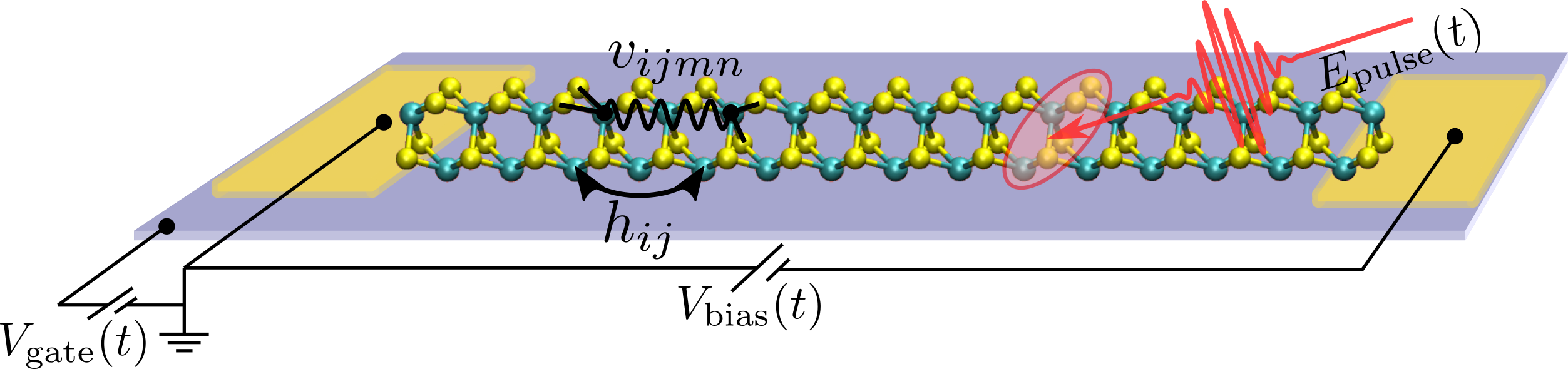
Figure 1: Quantum transport set up. A nanowire (finite quantum system) is contacted to left ($\alpha=L$) and right ($\alpha=R$) electrodes and lies over a substrate (or gate electrode) $\alpha=$gate. The nanowire is driven out of equilibrium by time dependent voltages $V_{\alpha}(t)$ [$V_{\rm bias}=V_{L}-V_{R}$] and laser pulses $E_{\rm pulse}(t)$.

Kadanoff-Baym equations for open systems.– We consider a finite quantum system, being it a molecule or a nanostructure, with one-electron integrals $h_{ij}(t)$ and two-electron integrals $v_{ijmn}$ in some orthonormal one-particle basis of dimension $N_{\rm sys}$, see Fig. 1. The time-dependence of $h_{ij}(t)=h^{0}_{ij}+\langle i|V_{\rm gate}(t)+\hat{\mathbf{d}}\cdot{\mathbf{E}_{\rm pulse}}(t)|j\rangle$ is due to a time-dependent gate voltage $V_{\mathrm{gate}}(t)$ and to a possible laser pulse $\mathbf{E}_{\rm pulse}(t)$ coupled to the electronic dipole operator $\hat{\mathbf{d}}$. The system is said open if it is in contact with electronic reservoirs with which it can exchange particles and hence energy. This is the typical quantum transport set up, the finite system being the junction and the electronic reservoirs being the electrodes. Neglecting correlation effects in the electrodes and between the electrodes and the system the Green’s function $G_{ij}(z,z^{\prime})$ with times $z,z^{\prime}$ on the Keldysh contour $C$ satisfies the equation of motion (EOM) (in the $N_{\rm sys}\times N_{\rm sys}$ matrix form) Jauho et al. (1994); Haug and Jauho (2008); Myöhänen et al. (2008, 2009); Stefanucci and van Leeuwen (2013)

$$\left[{\rm i}\frac{d}{dz}-h^{e}(z)\right] G(z,z^{\prime})=\delta(z,z^{\prime})$$

$$+\!\int_{C}d\bar{z}\;\big{[}\Sigma_{\rm c}(z,\bar{z})+\ \Sigma_{\rm em}(z,\bar{z})\big{]}G(\bar{z},z^{\prime}).$$ (1)

In Eq. (1) $h^{e}_{ij}(z)=h_{ij}(z)+V^{\rm HF}_{ij}(z)$ is the one-electron Hamiltonian properly renormalized by the Hartree-Fock (HF) potential $V^{\rm HF}_{ij}(z)=-i\sum_{mn}(v_{imnj}-v_{imjn})G_{nm}(z,z^{+})$, $\Sigma_{\rm c}$ is the correlation self-energy due to electron-electron interactions, and $\Sigma_{\rm em}$ is the embedding self-energy accounting for all virtual processes where an electron from orbital $i$ leaves the system to occupy some energy level in one of the electrodes and thereafter moves back to the system in orbital $j$.

The Kadanoff-Baym equations (KBE) for the open system follow from Eq. (1) by choosing the times $z$ and $z^{\prime}$ on different branches of the Keldysh contour Stefanucci and van Leeuwen (2013). In particular the EOM for the $N_{\rm sys}\times N_{\rm sys}$ electronic density matrix $\rho(t)=-iG(z,z^{+})=-iG^{<}(t,t)$ can easily be derived by subtracting Eq. (1) from its adjoint and then setting $z=t$ on the forward branch and $z^{\prime}=t$ on the backward branch:

$$i\frac{d}{dt}\rho(t)=\Big{(}h^{e}(t)\rho(t)-iI_{\rm c}(t)-iI_{\rm em}(t)\Big{)}-{\rm h.c.}.$$ (2)

The collision integral $I_{\rm c}$ is the convolution between the correlation self-energy and the Green’s function $G$ whereas the embedding integral $I_{\rm em}$, the main focus of this work, is the convolution between the embedding self-energy and $G$. For $I_{\rm em}=0$ the system is closed (no electrodes) and the KBE have been implemented in a number of works using different approximations to $\Sigma_{\rm c}$; these include the second-Born Dahlen and van Leeuwen (2007); Balzer et al. (2012), the $GW$ and $T$-matrix von Friesen et al. (2009); Stan et al. (2009); Puig von Friesen et al. (2010); Schüler et al. (2020), the Fan-Migdal Säkkinen et al. (2015); Schüler et al. (2016), and approximations based on the nonequilibrium dynamical mean-field theory Freericks et al. (2006); Aoki et al. (2014); Strand et al. (2015); Golež et al. (2017). KBE studies of open systems are less numerous Myöhänen et al. (2008, 2009); Puig von Friesen et al. (2010). In all cases the unfavorable $O(N_{t}^{3})$ scaling with the number of time steps $N_{t}$ limits the KBE, and hence the possibility of studying ultrafast correlated dynamics, to relatively small systems, although promising progresses have been recently achieved Schüler et al. (2020); Kaye and Golež (2021); Meirinhos et al. (2022); Dong et al. (2022).

Generalized Kadanoff-Baym Ansatz.– For any given correlation self-energy the direct solution of the EOM for the density matrix, see Eq. (2), is computationally less complex than solving the KBE and opens the door to a wealth of nonequilibrium phenomena Perfetto and Stefanucci (2018). To date the most efficient way to make the collision integral a functional of $\rho$ is the Generalized Kadanoff-Baym Ansatz (GKBA) Lipavský et al. (1986) with $G^{R/A}$ the $N_{\rm sys}\times N_{\rm sys}$ retarded/advanced quasi-particle propagators, $\rho^{>}=\rho-1$ and $\rho^{<}=\rho$. The GKBA respects the causal structure and it preserves all fundamental conservation laws for $\Phi$-derivable approximations Baym (1962) to $\Sigma_{\rm c}$ Karlsson et al. (2021). In closed systems the GKBA-EOM can be exactly reformulated in terms of a coupled set of ODEs Schlünzen et al. (2020); Joost et al. (2020) for several major approximations to $\Sigma_{\rm c}$, the most notable being $GW$ and $T$-matrix Schlünzen et al. (2020); Joost et al. (2020); Perfetto et al. (2022), $GW$ and $T$-matrix plus exchange Pavlyukh et al. (2021, 2022a), Fan-Migdal Karlsson et al. (2021) and the doubly-screened $G\widetilde{W}$ Pavlyukh et al. (2022b). In essence, the idea is to introduce high-order correlators $\mbox{$\mathcal{G}$}^{a=1,\ldots,n}(t)$ ($\mbox{$\mathcal{G}$}^{1}=\rho$), write $I_{\rm c}[\{\mbox{$\mathcal{G}$}^{a}\}]$ as a functional of them, and solve the coupled EOMs $i\frac{d}{dt}\mbox{$\mathcal{G}$}^{a}=\mbox{$\mathcal{I}$}^{a}[\{\mbox{$\mathcal{G}$}^{a}\}]$ ($\mbox{$\mathcal{I}$}^{1}=\big{(}h^{e}\rho-iI_{\rm c}\big{)}-{\rm h.c.}$). For all aforementioned methods the system of ODE can be closed using a relatively few number of correlators (the highest number being $n=7$ in $G\widetilde{W}$). Extending the ODE formulation to open systems would enable performing time-linear ($O(N_{t})$ scaling) NEGF simulations of correlated junctions and hence studying, e.g., the formation of Kondo singlets Krivenko et al. (2019), blocking dynamics of polarons Albrecht et al. (2013); Wilner et al. (2014a), bistability and hysteresis Galperin et al. (2005); Wilner et al. (2013), phonon dynamics and heating Galperin et al. (2007a, b); Wilner et al. (2014b); Rizzi et al. (2016), nonconservative dynamics Todorov et al. (2001); Dundas et al. (2009); Bode et al. (2011); Chen et al. (2019), molecular electroluminescence Miwa et al. (2019) as well as transport and optical response of junctions under periodic drivings Cabra et al. (2020); Zheng et al. (2013), see also Ref. Ridley et al. (2022) for a recent review.

Below we show that the set of ODEs for closed systems can be coupled to one more ODE for the embedding correlator $\mbox{$\mathcal{G}$}^{\rm em}$ to effectively open the system, thus providing a time-linear method to solve Eq. (2). Equation (2) was originally investigated using the integral (convolution) form of the collision and embedding integrals in Refs. Latini et al. (2014); Tuovinen et al. (2020, 2021); Tuovinen (2021). It was emphasized therein that the GKBA propagators $G^{R/A}$ chosen for closed-system simulations need to be modified. This change affects all other ODEs in an extremely elegant way while preserving the overall computational complexity.

Time-linear method.– Let $\Sigma_{\alpha}$ be the embedding self-energy of electrode $\alpha=1,\ldots,N_{\rm leads}$, hence $\Sigma_{\rm em}=\sum_{\alpha}\Sigma_{\alpha}$. In the so-called wide-band limit approximation (WBLA) wbl , the retarded and lesser components read Stefanucci and van Leeuwen (2013); Tuovinen et al. (2014); sup

$$\Sigma^{R}_{\alpha}(t,t^{\prime}) =-\frac{i}{2}s^{2}_{\alpha}(t)\delta(t,t^{\prime})\,\Gamma_{\alpha},$$ (3a)

$$\Sigma^{<}_{\alpha}(t,t^{\prime}) =is_{\alpha}(t)s_{\alpha}(t^{\prime})e^{-i\phi_{\alpha}(t,t^{\prime})}\!\!\int\!\!\frac{d\omega}{2\pi}f(\omega-\mu)e^{-i\omega(t-t^{\prime})}\,\Gamma_{\alpha},$$ (3b)

where $s_{\alpha}(t)$ is the switch-on function for the contact between the system and electrode $\alpha$, $\Gamma_{\alpha}$ is the $N_{\rm sys}\times N_{\rm sys}$ quasi-particle line-width matrix due to electrode $\alpha$, $\phi_{\alpha}(t,t^{\prime})\equiv\int_{t^{\prime}}^{t}d\bar{t}\;V_{\alpha}(\bar{t})$ is the accumulated phase due to the time-dependent voltage $V_{\alpha}$ Ridley et al. (2015), and $f(\omega-\mu)=1/(e^{\beta(\omega-\mu)}+1)$ is the Fermi function at inverse temperature $\beta$ and chemical potential $\mu$. The matrix elements $\Gamma_{\alpha,ij}=2\pi\sum_{k}T_{ik\alpha}\delta(\mu-\epsilon_{k\alpha})T_{k\alpha j}$ can be calculated from the transition amplitudes $T_{k\alpha j}=T^{\ast}_{jk\alpha}$ from orbital $j$ to level $k$ in electrode $\alpha$ having the energy dispersion $\epsilon_{k\alpha}$. The exact form of the embedding integral is then

$$I_{\rm em}(t)=\sum_{\alpha}I_{\alpha}(t)=\int\!\!d\bar{t}\;\Sigma^{<}_{\rm em}(t,\bar{t})G^{A}(\bar{t},t)+\frac{1}{2}\Gamma(t)\rho(t),$$ (4)

with $\Gamma(t)\equiv\sum_{\alpha}s^{2}_{\alpha}(t)\Gamma_{\alpha}$. In Ref. Latini et al. (2014) it was shown that the mean-field approximation of Eq. (2), i.e., $I_{\rm c}=0$, is exactly reproduced in GKBA provided that

$$G^{R}(t,t^{\prime})=-i\theta(t-t^{\prime})Te^{-i\int_{t^{\prime}}^{t}d\bar{t}\big{(}h^{e}(\bar{t})-i\Gamma(\bar{t})/2\big{)}},$$ (5)

and $G^{A}(t^{\prime},t)=[G^{R}(t,t^{\prime})]^{{\dagger}}$. Equation (5) reduces to the propagator of closed systems for $\Gamma=0$. In open systems, however, setting $\Gamma=0$ is utterly inadequate as no steady-state would ever be attained. Beyond the mean-field approximation we close Eq. (2) using the GKBA with propagators as in Eq. (5) pro .

To construct the time-linear method we use an efficient pole expansion (PE) scheme for the Fermi function Hu et al. (2010) $f(\omega)=\frac{1}{2}-\sum_{l}\eta_{l}\left(\frac{1}{\beta\omega+i\zeta_{l}}+\frac{1}{\beta\omega-i\zeta_{l}}\right)$, ${\rm Re}[\zeta_{l}]>0$, to rewrite the lesser self-energy for $t>t^{\prime}$ as $\Sigma_{\alpha}^{<}(t,t^{\prime})=\frac{i}{2}s_{\alpha}^{2}(t)\delta(t-t^{\prime})\Gamma_{\alpha}-s_{\alpha}(t)\sum_{l}\frac{\eta_{l}}{\beta}F_{l\alpha}(t,t^{\prime})\Gamma_{\alpha}$ with

$$F_{l\alpha}(t,t^{\prime})=s_{\alpha}(t^{\prime})e^{-i\phi_{\alpha}(t,t^{\prime})}e^{-i(\mu-i\frac{\zeta_{l}}{\beta})(t-t^{\prime})}.$$ (6)

Inserting the result into Eq. (4) the EOM Eq. (2) for the density matrix becomes

$$i\frac{d}{dt}\rho =\Big{(}h^{e}_{\rm eff}\rho+\frac{i}{4}\Gamma+i\sum_{l\alpha}s_{\alpha}\frac{\eta_{l}}{\beta}\Gamma_{\alpha}\mbox{$\mathcal{G}$}^{\rm em}_{l\alpha}-iI_{\rm c}\Big{)}-{\rm h.c.},$$ (7)

where $h^{e}_{\rm eff}(t)\equiv h^{e}(t)-i\Gamma(t)/2$ is the effective (non-self-adjoint) mean-field Hamiltonian and $\mbox{$\mathcal{G}$}^{\rm em}_{l\alpha}(t)\equiv\int\!\!d\bar{t}\;F_{l\alpha}(t,\bar{t})G^{A}(\bar{t},t)$ is the $N_{\rm sys}\times N_{\rm sys}$ embedding correlator. Taking into account the explicit expressions in Eqs. (5) and (6) we find

$$\!\!i\frac{d}{dt}\mbox{$\mathcal{G}$}^{\rm em}_{l\alpha}(t)=-s_{\alpha}(t)-\mathcal{G}^{\rm em}_{l\alpha}(t)\Big{(}h^{e{\dagger}}_{\rm eff}(t)-V_{\alpha}(t)-\mu+i\frac{\zeta_{l}}{\beta}\Big{)}.$$ (8)

Equations (7) and (8), together with the ODEs for $I_{\rm c}$, form a coupled system of ODEs for correlated real-time simulations of open systems. This time-linear method becomes similar to the one of Refs. Croy and Saalmann (2009); Zheng et al. (2010); Zhang et al. (2013); Kwok et al. (2013); Wang et al. (2013); Kwok et al. (2019) for $I_{\rm c}=0$. The scaling with the system size of Eq. (8) grows like $N_{\rm sys}^{3}\times N_{p}\times N_{\rm leads}$ where $N_{p}$ is the number of poles for the expansion of $f(\omega)$ sup .

An alternative time-linear method can be constructed from the spectral decomposition (SD) of the embedding self-energy $\Sigma_{\alpha,ij}(z,z^{\prime})=s_{\alpha}(z)s_{\alpha}(z^{\prime})\sum_{k}T_{ik\alpha}g_{k\alpha}(z,z^{\prime})T_{k\alpha j}$, where $g_{k\alpha}$ is the Green’s function of the isolated electrode. In this case, one would rewrite the embedding integral as $I_{{\rm em},ij}=\sum_{k\alpha}T_{ik\alpha}\widetilde{\mbox{$\mathcal{G}$}}^{\rm em}_{k\alpha j}$ and derive an ODE for the scalar quantities $\widetilde{\mbox{$\mathcal{G}$}}^{\rm em}_{k\alpha j}=\sum_{m}\int d\bar{t}[g^{R}_{ka}(t,\bar{t})T_{kam}G^{<}_{mj}(\bar{t},t)+g^{<}_{ka}(t,\bar{t})T_{k\alpha m}G^{A}_{mj}(\bar{t},t)]$ using the GKBA for the lesser Green’s function. The scaling with the system size of the scalar ODE for all $\widetilde{\mbox{$\mathcal{G}$}}^{\rm em}_{k\alpha j}$ grows like $N_{\rm sys}^{2}\times N_{k}\times N_{\rm leads}$ sup , where $N_{k}$ is the number of $k$-points needed for the discretization. The SD scheme is ill-advised for the following reasons. If the electrodes are not wide band then the calculation of the mean-field propagator scales cubically in time; any other approximation to $G^{R}$, including Eq. (5), would be inconsistent and could even lead to unphysical time evolutions, e.g., no steady states for constant voltages. If the electrodes are wide band then $N_{k}$ could be orders of magnitude larger than $N_{\rm sys}\times N_{p}$ to achieve convergence, hence $N_{\rm sys}^{2}\times N_{k}\gg N_{\rm sys}^{3}\times N_{p}$. This statement is proven numerically below; see also Supplemental Material sup .

The quasi-particle broadening $\Gamma$ in the propagators, see Eq. (5), is only responsible for a minor change in the ODEs for the high-order correlators of closed systems. We focus here on the $T$-matrix approximation in the particle-hole channel ($T^{ph}$) as $T^{ph}$-simulations of open systems are reported below; similar arguments apply to all other approximations in Ref. Pavlyukh et al. (2022b). The collision integral is $I_{{\rm c},ij}=-i\sum_{lmn}v_{inml}\mbox{$\mathcal{G}$}^{\rm c}_{lmjn}$ where $\mbox{$\mathcal{G}$}^{\rm c}_{lmjn}=-\langle\hat{d}^{{\dagger}}_{j}\hat{d}^{{\dagger}}_{n}\hat{d}_{l}\hat{d}_{m}\rangle_{\rm c}$ is the correlated part of the equal-time two-particle Green’s function Stefanucci and van Leeuwen (2013). Following Refs. Pavlyukh et al. (2021, 2022a), we construct the matrices in the two-electron space $\mbox{\boldmath$\mathcal{G}$}^{\rm c}_{\begin{subarray}{c}ij\\ nm\end{subarray}}(t)\equiv\mbox{$\mathcal{G}$}^{\rm c}_{imjn}(t)$, $\mbox{\boldmath$v$}_{\begin{subarray}{c}ij\\ nm\end{subarray}}\equiv v_{imnj}$ and $\mbox{\boldmath$\rho$}^{\lessgtr}_{\begin{subarray}{c}ij\\ nm\end{subarray}}\equiv\rho^{\lessgtr}_{ij}\rho^{\gtrless}_{mn}$ (boldface letters are used to distinguish them from matrices in one-electron space). The only difference in the derivation of the EOM for $\mathcal{G}$ of closed systems Pavlyukh et al. (2021, 2022a) comes from the fact that the EOM for the propagator contains $h^{e}_{\rm eff}$ instead of $h^{e}$. The final result is therefore

$$i\frac{d}{dt}\mbox{\boldmath$\mathcal{G}$}^{\rm c}=\Big{(}\mbox{\boldmath$\rho$}^{<}\mbox{\boldmath$v$}\mbox{\boldmath$\rho$}^{>}+\big{(}\mbox{\boldmath$h$}^{e}_{\rm eff}+\mbox{\boldmath$\rho$}^{\Delta}\mbox{\boldmath$v$}\big{)}\mbox{\boldmath$\mathcal{G}$}^{\rm c}\Big{)}-{\rm h.c.},$$ (9)

where $\mbox{\boldmath$\rho$}^{\Delta}=\mbox{\boldmath$\rho$}^{>}-\mbox{\boldmath$\rho$}^{<}$ and ${\mbox{\boldmath$h$}^{e}_{\mathrm{eff},}}_{\begin{subarray}{c}ij\\ nm\end{subarray}}\equiv h^{e}_{{\rm eff},ij}\delta_{mn}-\delta_{ij}h^{e{\dagger}}_{{\rm eff},nm}$. The solution of the coupled ODEs for $\rho$, $\mbox{$\mathcal{G}$}^{\rm em}$ and $\mbox{$\mathcal{G}$}^{\rm c}$ yields the time-dependent evolution of open systems in the $T^{ph}$ approximation. Similarly, one can show that all the 2¹² NEGF methods of Ref. Pavlyukh et al. (2022b) are only affected by the replacement $h^{e}\to h^{e}_{\rm eff}$. The addition of $I_{\rm em}$ in the EOM for $\rho$ along with the propagation of the embedding correlator according to Eq. (8), allows for studying open systems for a large number of NEGF methods. These include methods to deal with the electron-phonon interaction as well Karlsson et al. (2021). Noteworthily, all NEGF methods in Ref. Pavlyukh et al. (2022b) guarantee the satisfaction of fundamental conservation laws like the continuity equation and the energy balance.

Charge current.– Charge distributions, local currents, local moments, etc., can be extracted from the one-particle density matrix $\rho$. Information on the electron-hole pair correlation function is carried by the $T^{ph}$ correlator $\mbox{$\mathcal{G}$}^{\rm c}$. The embedding correlator $\mbox{$\mathcal{G}$}^{\rm em}$ is instead crucial for calculating the time-dependent current $J_{\alpha}(t)$ at the interface between the system and electrode $\alpha$. This current is given by the Meir-Wingreen formula Meir and Wingreen (1992) and it can be written as the contribution of the $\alpha$ electrode to the embedding integral Jauho et al. (1994); Haug and Jauho (2008); Stefanucci and van Leeuwen (2013), see Eq. (4), $J_{\alpha}(t)=2{\rm Re}{\rm Tr}[I_{\alpha}(t)]$. Expressing the embedding self-energy in terms of $\mbox{$\mathcal{G}$}^{\rm em}$ we find

$$\!\!\!J_{\alpha}(t)=2s_{\alpha}(t){\rm Re}{\rm Tr}\Big{[}\Gamma_{\alpha}\Big{(}\!s_{\alpha}(t)\frac{2\rho(t)-1}{4}-\!\sum_{l}\frac{\eta_{l}}{\beta}\mbox{$\mathcal{G}$}^{\rm em}_{l\alpha}(t)\!\Big{)}\Big{]}.$$ (10)

Satisfaction of the continuity equation implies $\mathrm{CE}\equiv\frac{d}{dt}{\rm Tr}[\rho]+\sum_{\alpha}J_{\alpha}=0$.

Spectral decomposition vs pole expansion.– We first study a two-level molecule coupled to two one-dimensional tight-binding electrodes. We set $h_{11}=h_{22}=0$, $h_{12}=h_{21}=-T/2$ and measure all energies in units of $T>0$. We consider an interaction $v_{ijmn}=v_{ij}\delta_{in}\delta_{jm}$ with $v_{11}=v_{22}=1$ and $v_{12}=v_{21}=0.5$. The chemical potential is fixed at the middle of the HF gap of the uncontacted system, in our case $\mu=1$, and the inverse temperature is $\beta=100$. The electrodes are parameterized by on-site and hopping energies $a_{\alpha}=\mu$ (half-filled electrodes), $b_{\alpha}=-8$, respectively, the energy dispersion thus taking the form $\epsilon_{k\alpha}=a_{\alpha}-2|b_{\alpha}|\cos[\pi k/(N_{k}+1)]$, with $N_{k}$ the number of discretized $k$ points. The left and right electrodes are coupled to the first and second molecular levels, respectively, with transition amplitude $T_{\alpha}=-0.2$, $\alpha=L,R$. As $T_{\alpha}\ll b_{\alpha}$ the WBLA is accurate and one finds $\Gamma_{L,ij}=\delta_{i1}\delta_{j1}\gamma_{L}$ and $\Gamma_{R,ij}=\delta_{i2}\delta_{j2}\gamma_{R}$ with $\gamma_{\alpha}=2T^{2}_{\alpha}/|b_{\alpha}|=0.01$.

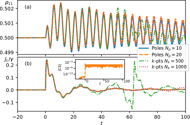
Figure 2: Dynamics of the two-level molecule contacted to a left and right electrodes. Occupation of the first level (a) and current at the left interface (b) using the SD ($k$-points $N_{k}$) and PE (poles $N_{p}$) schemes. The inset in panel (b) shows the continuity equation $\mathrm{CE}=\frac{d}{dt}\mathrm{Tr}[\rho]+\sum_{\alpha}J_{\alpha}$. Energies in units of $T$ and time in units of $1/T$.

In Fig. 2 we present time-dependent HF results for the occupation of the first level [panel (a)] and the current at the left interface [panel (b)]. We adiabatically switch on the contacts between the molecule and the electrodes for $t<0$ with a “sine-squared” switch-on function Karlsson et al. (2018), and then drive the system away from equilibrium with a constant bias $V_{L}=T/2$, $V_{R}=0$ for $t\geq 0$ (hence $V_{\mathrm{gate}}=0$, $E_{\mathrm{pulse}}=0$, $V_{\mathrm{bias}}=V_{L}-V_{R}$). The time-linear PE and SD schemes perform similarly at convergence, as they should. However, within the time-frame of the simulation, $N_{k}=1000$ $k$-points are needed to converge the SD scheme, against only $N_{p}=20$ poles needed to converge the PE scheme. Furthermore, the convergence with $N_{p}$ is independent of the maximum simulation time whereas $N_{k}$ must grow linearly with it for otherwise finite size effects, as those visible for $N_{k}=500$ at time $t\simeq 50$, take place. Steady values are attained on a time scale of a few $1/\gamma_{a}$ time units sup . The inset in Fig. 2(b) shows that the continuity equation is satisfied with high accuracy.

Correlated electron-hole transport.– Transport of correlated electron-holes ($eh$) is a fundamental process in photovoltaic junctions Ponseca et al. (2017); Pastor et al. (2019). We study the relaxation of a suddenly created $eh$ in a two-band direct gap one-dimensional semiconductor coupled to WBLA electrodes. The Hamiltonian of the system reads $\hat{H}=\sum_{ij\nu}h_{ij\nu}\hat{d}_{i\nu}^{\dagger}\hat{d}_{j\nu}+U\sum_{i}\hat{n}_{iv}\hat{n}_{ic}$, where $\hat{d}_{i\nu}$ destroys an electron in the $i$-th valence ($\nu=v$) or conduction ($\nu=c$) orbital, and $\hat{n}_{i\nu}\equiv\hat{d}_{i\nu}^{\dagger}\hat{d}_{i\nu}$ is the orbital occupation. The one-electron integrals are $h_{iiv}=-\epsilon_{0}<0$, $h_{iic}=\epsilon_{0}-U$ on site and $h_{ijv}=-h_{ijc}=T>0$ for nearest neighbors Perfetto et al. (2019). In equilibrium the HF gap is $\Delta=2(\epsilon_{0}-2T)$. The left and right electrodes are coupled to the left- and right-most orbitals, respectively, with tunneling strength $\gamma_{\alpha}$ independent of $\alpha$. Henceforth all energies are measured in units of $\Delta/2$; we set $\epsilon_{0}=4.5$, $T=1.75$, $\gamma_{\alpha}=0.1$ and work at inverse temperature $\beta=100$. The equilibrium chemical potential is set in the middle of the HF gap of the uncontacted system.

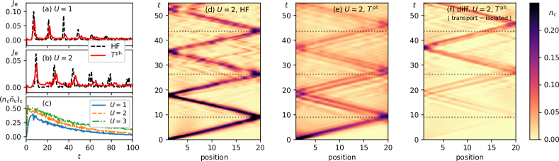
Figure 3: Dynamics of an electron-hole pair in a one-dimensional semiconductor junction with $N=20$ cells. (a-b) Time-dependent current at the right-interface in HF (dashed) and $T^{ph}$ (solid) for $U=1$ (a) and $U=2$ (b). (c) Correlated part of the total number of $eh$ pairs for different interaction strengths. (d-e) Conduction occupations (color map) versus time (vertical axis) and cell position (horizontal axis) in HF (d) and $T^{ph}$ (e). (f) Difference of panel (e) to a situation without electrodes. The dashed lines are guides to the eye.

At time $t=0$ we suddenly couple the system to the electrodes and create an $eh$ excitation at the left-most orbitals, hence $\rho_{iv,iv}(0)=(1-\delta_{i1})$ and $\rho_{ic,ic}(0)=\delta_{i1}$. In Fig. 3(a) and (b), we show the current at the right interface in two different many-body methods, i.e., HF and $T^{ph}$, and for two values $U=1,2$ of the $eh$ attraction. The results indicate that: (i) the velocity of the $eh$ wavepacket is faster in HF than $T^{ph}$ (each spike corresponds to an $eh$ bouncing at the right interface); (ii) the HF dynamics is coherent, the wavepacket travelling almost undisturbed, whereas in $T^{ph}$ correlations are responsible for a fast decoherence and wavepacket spreading. The slower velocity in $T^{ph}$ is rationalized in Fig. 3(c) where we plot the correlated part of the total number of $eh$ pairs: $\sum_{i}\langle(1-\hat{n}_{iv})\hat{n}_{ic}\rangle_{\rm c}=-\sum_{i}\mbox{$\mathcal{G}$}^{\rm c}_{icivivic}$. The build-up of correlations is almost instantaneous. The initially uncorrelated $eh$ pair binds and becomes heavier, thus reducing the propagation speed. The observed decay at longer times is due to electron and hole tunneling into the electrodes; at the steady state about $10^{-2}$ conduction electrons and valence holes remain in the system (not shown). Both decoherence and velocity reduction are well visible in Fig. 3(d) and (e) where we display the color plot of the conduction occupations $n_{ic}(t)=\rho_{ic,ic}(t)$ in HF and $T^{ph}$ for $U=2$. In $T^{ph}$ the $eh$ wavepacket loses coherence and spreads after bouncing back and forth a few times. In Fig. 3(f) we analyze the effect of the electrodes by showing the difference between the open and closed system dynamics. In the open system the amplitude of the wavepacket and the localization of the charge decreases faster than in the isolated system.

In conclusion, we put forward a time-linear approach to study the correlated dynamics of open systems with a large number of NEGF methods. Our work empowers the Meir-Wingreen formula allowing its use in contexts and/or for levels of approximation which were previously unattainable in practice. The ODE formulation lends itself to parallel computation, adaptive time-stepping implementations and restart protocols, thus opening new avenues for the ab initio description of time-dependent quantum transport phenomena.

Supplemental Material for “Time-linear quantum transport simulations with correlated nonequilibrium Green’s functions”

In this Supplemental Material, we consider only the embedding self-energy between the system and the electrodes. Other collision terms, such as electron-electron and electron-phonon interactions, can be taken care of by a separate calculation Karlsson et al. (2021); Pavlyukh et al. (2022).

I Quantum transport setup

We consider the following Hamiltonian for the quantum-correlated system coupled to electrodes

$$\hat{H} =\sum_{k\alpha,\sigma}\epsilon_{k\alpha}\hat{d}_{k\alpha,\sigma}^{\dagger}\hat{d}_{k\alpha,\sigma}+\sum_{ij,\sigma}h_{ij}\hat{d}_{i,\sigma}^{\dagger}\hat{d}_{j,\sigma}$$

$$+\sum_{ik\alpha,\sigma}\left(T_{ik\alpha}\hat{d}_{i,\sigma}^{\dagger}\hat{d}_{k\alpha,\sigma}+\text{h.c.}\right)$$

$$+\frac{1}{2}\sum_{\begin{subarray}{c}ijmn\\ \sigma\sigma^{\prime}\end{subarray}}v_{ijmn}\hat{d}_{i,\sigma}^{\dagger}\hat{d}_{j,\sigma^{\prime}}^{\dagger}\hat{d}_{m,\sigma^{\prime}}\hat{d}_{n,\sigma},$$ (1)

where $\hat{d}^{(\dagger)}$ are the electronic annihilation (creation) operators, $\epsilon_{k\alpha}$ is the energy dispersion of the $\alpha$-th electrode, $h_{ij}$ are the one-particle matrix elements of the system, $T_{ik\alpha}$ are the tunneling matrix elements between the system and the electrodes, and $v_{ijmn}$ are the Coulomb integrals of the system. An out-of-equilibrium condition, making charge carriers to flow through the system, is introduced by assigning time-dependence on the horizontal branch of the Keldysh contour, $\epsilon_{k\alpha}\to\epsilon_{k\alpha}+V_{\alpha}(t)\equiv\bar{\epsilon}_{k\alpha}(t)$, $h_{ij}\to h_{ij}(t)$, and $T_{ik\alpha}\to T_{ik\alpha}s_{\alpha}(t)$, where $V_{\alpha}(t)$ is the (time-dependent) bias-voltage profile, and $s_{\alpha}(t)$ is a switch-on function for the system-electrode coupling. While the two-body interaction is itself instantaneous, we could also ramp the strength of the Coulomb integrals with a switch-on function.

II Retarded self-energy and the effective Hamiltonian

The retarded self-energy appears in the equation of motion for the retarded Green’s function:

$$\left[{\rm i}\frac{{\rm d}}{{\rm d}t}-h^{e}(t)\right]G^{\text{R}}(t,t^{\prime})=\delta(t,t^{\prime})+\int{\rm d}\bar{t}\Sigma^{\text{R}}(t,\bar{t})G^{\text{R}}(\bar{t},t^{\prime}),$$ (2)

where $h^{e}(t)$ is the (time-dependent) one-electron Hamiltonian, including the Hartree-Fock potential. The self-energy is constructed from the tunneling matrices and the electrode Green’s function as $\Sigma^{\text{R}}(t,t^{\prime})=\sum_{\alpha}\Sigma^{\text{R}}_{\alpha}(t,t^{\prime})$ with Tuovinen et al. (2014)

$$\Sigma_{\alpha,ij}^{\text{R}}(t,t^{\prime})=\sum_{k}T_{ik\alpha}s_{\alpha}(t)g_{k\alpha}^{\text{R}}(t,t^{\prime})T_{k\alpha j}s_{\alpha}(t^{\prime}),$$ (3)

where we assumed the tunneling strength between the system and electrode $\alpha$ depends on time only through an overall switch-on function $s_{\alpha}(t)$. The free-electron, retarded Green’s function of the $\alpha$-th electrode is

$$g_{k\alpha}^{\text{R}}(t,t^{\prime})=-{\rm i}\theta(t-t^{\prime}){\rm e}^{-{\rm i}\phi_{\alpha}(t,t^{\prime})}{\rm e}^{-{\rm i}\epsilon_{k\alpha}(t-t^{\prime})}$$ (4)

with $\epsilon_{k\alpha}$ and $\phi_{\alpha}(t,t^{\prime})\equiv\int_{t^{\prime}}^{t}{\rm d}\bar{t}V_{\alpha}(\bar{t})$ the energy dispersion and the bias-voltage phase factor, respectively. Inserting this into the expression for the self-energy, we can transform the $k$-summation into a frequency integral as

$$\Sigma_{\alpha,ij}^{\text{R}}(t,t^{\prime}) =-{\rm i}s_{\alpha}(t)s_{\alpha}(t^{\prime}){\rm e}^{-{\rm i}\phi_{\alpha}(t,t^{\prime})}\int\frac{{\rm d}\omega}{2\pi}{\rm e}^{-{\rm i}\omega(t-t^{\prime})}$$

$$\hskip 50.0pt\times 2\pi\sum_{k}T_{ik\alpha}\delta(\omega-\epsilon_{k\alpha})T_{k\alpha j}\theta(t-t^{\prime})$$

$$=-\frac{{\rm i}}{2}s_{\alpha}^{2}(t)\delta(t-t^{\prime})\Gamma_{\alpha,ij},$$ (5)

where we employed the wide-band limit approximation (WBLA), $\Gamma_{\alpha,ij}(\omega)=2\pi\sum_{k}T_{ik\alpha}\delta(\omega-\epsilon_{k\alpha})T_{k\alpha j}\simeq\Gamma_{\alpha,ij}(\mu)\equiv\Gamma_{\alpha,ij}$, and we used $\int\frac{{\rm d}\omega}{2\pi}{\rm e}^{-{\rm i}\omega(t-t^{\prime})}\theta(t-t^{\prime})=\delta(t-t^{\prime})/2$. Inserting this into the r.h.s. of Eq. (2) we obtain

$$\int{\rm d}\bar{t}\Sigma^{\text{R}}(t,\bar{t})G^{\text{R}}(\bar{t},t^{\prime}) =\int{\rm d}\bar{t}\sum_{\alpha}[-{\rm i}\Gamma_{\alpha}s_{\alpha}^{2}(t)/2]\delta(t-\bar{t})G^{\text{R}}(\bar{t},t^{\prime})$$

$$=-\frac{{\rm i}}{2}\sum_{\alpha}\Gamma_{\alpha}s_{\alpha}^{2}(t)G^{\text{R}}(t,t^{\prime}),$$ (6)

so we may write the equation of motion as

$$\left[{\rm i}\frac{{\rm d}}{{\rm d}t}-h^{e}_{\text{eff}}(t)\right]G^{\text{R}}(t,t^{\prime})=\delta(t,t^{\prime})$$ (7)

with the non-self-adjoint, effective Hamiltonian $h^{e}_{\text{eff}}(t)\equiv h^{e}(t)-\frac{{\rm i}}{2}\sum_{\alpha}\Gamma_{\alpha}s_{\alpha}^{2}(t)$. When considering the GKBA for the lesser and greater Green’s functions,

$$G^{\lessgtr}(t,t^{\prime})=-G^{\text{R}}(t,t^{\prime})\rho^{\lessgtr}(t^{\prime})+\rho^{\lessgtr}(t)G^{\text{A}}(t,t^{\prime}),$$ (8)

we take the quasi-particle propagators for the coupled system as $G^{\text{R}/\text{A}}(t,t^{\prime})=\mp{\rm i}\theta[\pm(t-t^{\prime})]\mathrm{T}{\rm e}^{-{\rm i}\int_{t^{\prime}}^{t}{\rm d}\bar{t}h^{e}_{\text{eff}}(\bar{t})}$. Within the GKBA, the lesser and greater Green’s functions thus satisfy Karlsson et al. (2021)

$${\rm i}\frac{{\rm d}}{{\rm d}t}G^{\lessgtr}(t,t^{\prime}) =h^{e}_{\text{eff}}(t)G^{\lessgtr}(t,t^{\prime}),$$ (9)

$$-{\rm i}\frac{{\rm d}}{{\rm d}t^{\prime}}G^{\lessgtr}(t,t^{\prime}) =G^{\lessgtr}(t,t^{\prime})h^{e\dagger}_{\text{eff}}(t^{\prime}).$$ (10)

III Lesser self-energy

For the equations of motion for the one-particle density matrix, we also need the lesser self-energy Tuovinen et al. (2014):

$$\Sigma_{\alpha,ij}^{<}(t,t^{\prime})=\sum_{k}T_{ik\alpha}s_{\alpha}(t)g_{k\alpha}^{<}(t,t^{\prime})T_{k\alpha j}s_{\alpha}(t^{\prime}),$$ (11)

where the free-electron, lesser Green’s function of the $\alpha$-th electrode is

$$g_{k\alpha}^{<}(t,t^{\prime})={\rm i}f(\epsilon_{k\alpha}-\mu){\rm e}^{-{\rm i}\int_{t^{\prime}}^{t}{\rm d}\bar{t}[\epsilon_{k\alpha}+V_{\alpha}(\bar{t})]}.$$ (12)

Here, it is worth noting that the initial condition originates from the Matsubara component, i.e., the Fermi function contains the unbiased electrode energy dispersion shifted by the chemical potential Stefanucci and van Leeuwen (2013). Transforming the $k$-summation into a frequency integral gives

$$\Sigma_{\alpha,ij}^{<}(t,t^{\prime}) ={\rm i}s_{\alpha}(t)s_{\alpha}(t^{\prime}){\rm e}^{-{\rm i}\phi_{\alpha}(t,t^{\prime})}\int\frac{{\rm d}\omega}{2\pi}f(\omega-\mu){\rm e}^{-{\rm i}\omega(t-t^{\prime})}$$

$$\hskip 50.0pt\times 2\pi\sum_{k}T_{ik\alpha}\delta(\omega-\epsilon_{k\alpha})T_{k\alpha j}.$$ (13)

In matrix form, we may then write (employing again the WBLA) Ridley et al. (2017)

$$\Sigma_{\alpha}^{<}(t,t^{\prime})={\rm i}\Gamma_{\alpha}s_{\alpha}(t)s_{\alpha}(t^{\prime}){\rm e}^{-{\rm i}\phi_{\alpha}(t,t^{\prime})}\int\frac{{\rm d}\omega}{2\pi}f(\omega-\mu){\rm e}^{-{\rm i}\omega(t-t^{\prime})}.$$ (14)

Away from the time-diagonal, $t\neq t^{\prime}$, the integral is well-behaving, a divergence is arising however for $t=t^{\prime}$. At zero temperature one finds $\Sigma^{<}(t,t^{\prime}\sim t)\sim\frac{1}{t-t^{\prime}}-i\pi\delta(t-t^{\prime})$, see Eq. (11) in Ref. Stefanucci et al. (2008). This divergence is however harmless since in the EOM the self-energy is always convoluted with the Green’s function over time; see below. The time-linear scheme is “blind” to the divergence of the embedding self-energy since it is cast in terms of the embedding correlator, which is the integral of the power-law divergent part of $\Sigma^{<}$ and the advanced Green’s function.

The Fermi function can be evaluated employing a pole expansion Hu et al. (2010); Ridley et al. (2017)

$$f(x)\equiv\frac{1}{{\rm e}^{\beta x}+1}=\frac{1}{2}-\lim_{N_{p}\to\infty}\sum_{l=1}^{N_{p}}\eta_{l}\left(\frac{1}{\beta x+{\rm i}\zeta_{l}}+\frac{1}{\beta x-{\rm i}\zeta_{l}}\right),$$ (15)

where $\eta$ and $\pm{\rm i}\zeta$ are the residues and poles ($\zeta>0$), respectively. In the Matsubara case, one would take $\eta_{l}=1$ and $\zeta_{l}=\pi(2l-1)$, but the expansion can be optimized through the solution of an eigenvalue problem of a specific, tridiagonal matrix Hu et al. (2010). Because of the exponential ${\rm e}^{-{\rm i}\omega(t-t^{\prime})}$, the nontrivial part of the integral is closed on the lower-half complex plane for $t>t^{\prime}$ and on the upper-half complex plane for $t<t^{\prime}$:

$$\Sigma_{\alpha}^{<}(t,t^{\prime})$$

$$={\rm i}\Gamma_{\alpha}s_{\alpha}(t)s_{\alpha}(t^{\prime}){\rm e}^{-{\rm i}\phi_{\alpha}(t,t^{\prime})}\frac{1}{2}\int\frac{{\rm d}\omega}{2\pi}{\rm e}^{-{\rm i}\omega(t-t^{\prime})}$$

$$-{\rm i}\Gamma_{\alpha}s_{\alpha}(t)s_{\alpha}(t^{\prime}){\rm e}^{-{\rm i}\phi_{\alpha}(t,t^{\prime})}\sum_{l}\frac{\eta_{l}}{\beta}$$

$$\times\int\frac{{\rm d}\omega}{2\pi}\left(\frac{1}{\omega-\mu+{\rm i}\zeta_{l}/\beta}+\frac{1}{\omega-\mu-{\rm i}\zeta_{l}/\beta}\right){\rm e}^{-{\rm i}\omega(t-t^{\prime})}$$

$$=\frac{{\rm i}}{2}\Gamma_{\alpha}s_{\alpha}^{2}(t)\delta(t-t^{\prime})-{\rm i}\Gamma_{\alpha}s_{\alpha}(t)s_{\alpha}(t^{\prime}){\rm e}^{-{\rm i}\phi_{\alpha}(t,t^{\prime})}\sum_{l}\frac{\eta_{l}}{\beta}$$

$$\times\left[-{\rm i}{\rm e}^{-{\rm i}(\mu-{\rm i}\frac{\zeta_{l}}{\beta})(t-t^{\prime})}\theta(t-t^{\prime})+{\rm i}{\rm e}^{-{\rm i}(\mu+{\rm i}\frac{\zeta_{l}}{\beta})(t-t^{\prime})}\theta(t^{\prime}-t)\right],$$ (16)

where we noticed a missing prefactor $1/\beta$ in Ref. Ridley et al. (2017). In our situation, we only require the $t>t^{\prime}$ contribution:

$$\Sigma_{\alpha}^{<}(t,t^{\prime}) =\frac{{\rm i}}{2}s_{\alpha}^{2}(t)\delta(t-t^{\prime})\Gamma_{a}$$

$$-s_{\alpha}(t)\sum_{l}\frac{\eta_{l}}{\beta}s_{\alpha}(t^{\prime}){\rm e}^{-{\rm i}\phi(t,t^{\prime})}{\rm e}^{-{\rm i}(\mu-{\rm i}\zeta_{l}/\beta)(t-t^{\prime})}\Gamma_{a}.$$ (17)

We observe that the inclusion of finite number of poles removes the power-law divergence and makes the function numerically more tractable Ridley et al. (2017).

IV Embedding integral

Inserting Eq. (II) into the embedding integral appearing in Eq. (2) of the main text yields

$$I_{\text{em}}(t) =\int{\rm d}\bar{t}\left[\Sigma^{<}(t,\bar{t})G^{\text{A}}(\bar{t},t)+\Sigma^{\text{R}}(t,\bar{t})G^{<}(\bar{t},t)\right]$$

$$=\int{\rm d}\bar{t}\left\{\Sigma^{<}(t,\bar{t})G^{\text{A}}(\bar{t},t)+\frac{1}{2}\Gamma(t)\delta(t-\bar{t})[-{\rm i}G^{<}(\bar{t},t)]\right\}$$

$$=\int{\rm d}\bar{t}\Sigma^{<}(t,\bar{t})G^{\text{A}}(\bar{t},t)+\frac{1}{2}\Gamma(t)\rho(t),$$ (18)

where we defined $\Gamma(t)\equiv\sum_{\alpha}s_{\alpha}^{2}(t)\Gamma_{\alpha}$ and $\rho(t)\equiv-{\rm i}G^{<}(t,t)$. Further, inserting Eq. (III) gives

$$I_{\text{em}}(t) =\frac{1}{2}\Gamma(t)\rho(t)+\sum_{\alpha}\int{\rm d}\bar{t}\left\{\frac{{\rm i}}{2}s_{\alpha}^{2}(t)\delta(t-\bar{t})\Gamma_{\alpha}G^{\text{A}}(\bar{t},t)\right.$$

$$\left.-s_{\alpha}(t){\textstyle\sum_{l}}\frac{\eta_{l}}{\beta}s_{\alpha}(\bar{t}){\rm e}^{-{\rm i}\phi(t,\bar{t})}{\rm e}^{-{\rm i}(\mu-{\rm i}\zeta_{l}/\beta)(t-\bar{t})}\Gamma_{a}G^{\text{A}}(\bar{t},t)\right\}$$

$$=\frac{1}{2}\Gamma(t)\rho(t)-\frac{1}{4}\Gamma(t)-\sum_{l\alpha}s_{\alpha}(t)\frac{\eta_{l}}{\beta}\Gamma_{\alpha}\mathcal{G}_{l\alpha}^{\text{em}}(t),$$ (19)

where we introduced the embedding correlator

$$\mathcal{G}_{l\alpha}^{\text{em}}(t)=\int{\rm d}\bar{t}s_{\alpha}(\bar{t}){\rm e}^{-{\rm i}\phi_{\alpha}(t,\bar{t})}{\rm e}^{-{\rm i}\mu(t-\bar{t})}{\rm e}^{-\zeta_{l}(t-\bar{t})/\beta}G^{\text{A}}(\bar{t},t).$$ (20)

In Eq. (IV), the prefactor of the second term results from the implicit step function within the advanced Green’s function: $\int{\rm d}\bar{t}\delta(t-\bar{t})G^{\text{A}}(\bar{t},t)={\rm i}/2$.

V Equations of motion

With the above-derived embedding integral, the equation of motion for the electronic density matrix becomes (here we omit the collision integral $I_{\text{c}}$ resulting from, e.g., electron-electron or electron-phonon correlations; it can be directly included)

$${\rm i}\frac{{\rm d}}{{\rm d}t}\rho(t)$$

$$=\left[h^{e}(t)\rho(t)-{\rm i}I_{\text{em}}(t)\right]-\text{h.c.}$$

$$=\left[h^{e}(t)\rho(t)-\frac{{\rm i}}{2}\Gamma(t)\rho(t)+\frac{{\rm i}}{4}\Gamma(t)\right.$$

$$\hskip 20.0pt\left.+{\rm i}{\textstyle\sum_{l\alpha}}s_{\alpha}(t)\frac{\eta_{l}}{\beta}\Gamma_{\alpha}\mathcal{G}_{l\alpha}^{\text{em}}(t)\right]-\text{h.c.}$$

$$=\left[h^{e}_{\text{eff}}(t)\rho(t)+\frac{{\rm i}}{4}\Gamma(t)+{\rm i}\sum_{l\alpha}s_{\alpha}(t)\frac{\eta_{l}}{\beta}\Gamma_{\alpha}\mathcal{G}_{l\alpha}^{\text{em}}(t)\right]-\text{h.c.},$$ (21)

where we utilized the effective Hamiltonian. The equation of motion for the embedding correlator is derived as

$${\rm i}\frac{{\rm d}}{{\rm d}t}\mathcal{G}_{l\alpha}^{\text{em}}(t)$$

$$=\int{\rm d}\bar{t}s_{\alpha}(\bar{t})\left\{{\rm i}\frac{{\rm d}}{{\rm d}t}{\rm e}^{-{\rm i}\int_{\bar{t}}^{t}{\rm d}\tau\left[V_{\alpha}(\tau)+\mu-{\rm i}\zeta_{l}/\beta\right]}\right\}G^{\text{A}}(\bar{t},t)$$

$$-\int{\rm d}\bar{t}s_{\alpha}(\bar{t}){\rm e}^{-{\rm i}\int_{\bar{t}}^{t}{\rm d}\tau\left[V_{\alpha}(\tau)+\mu-{\rm i}\zeta_{l}/\beta\right]}\left\{-{\rm i}\frac{{\rm d}}{{\rm d}t}G^{\text{A}}(\bar{t},t)\right\}$$

$$=\int{\rm d}\bar{t}s_{\alpha}(\bar{t})\left[V_{\alpha}(t)+\mu-{\rm i}\zeta_{l}/\beta\right]{\rm e}^{-{\rm i}\int_{\bar{t}}^{t}{\rm d}\tau\left[V_{\alpha}(\tau)+\mu-{\rm i}\zeta_{l}/\beta\right]}G^{\text{A}}(\bar{t},t)$$

$$-\int{\rm d}\bar{t}s_{\alpha}(\bar{t}){\rm e}^{-{\rm i}\int_{\bar{t}}^{t}{\rm d}\tau\left[V_{\alpha}(\tau)+\mu-{\rm i}\zeta_{l}/\beta\right]}\left[G^{\text{A}}(\bar{t},t)h^{e\dagger}_{\text{eff}}(t)+\delta(\bar{t}-t)\right]$$

$$=-s_{\alpha}(t)-\mathcal{G}_{l\alpha}^{\text{em}}(t)\left[h^{e\dagger}_{\text{eff}}(t)-V_{\alpha}(t)-\mu+{\rm i}\zeta_{l}/\beta\right],$$ (22)

where we used the equation of motion (7) of the quasi-particle propagator for the coupled system $G^{\text{A}}(\bar{t},t)=[G^{\text{R}}(t,\bar{t})]^{\dagger}$.

The embedding correlator in Eq. (20) is a $N_{\text{sys}}\times N_{\text{sys}}$ matrix. The multiplication in Eq. (V) thus leads to an overall computational complexity $N_{\text{sys}}^{3}\times N_{p}\times N_{\rm leads}$.

VI $k$-resolved spectral decomposition

Alternatively, we could also write the embedding integral (IV) directly in terms of the $k$-resolved electrode Green’s functions (spectral decomposition):

$$I_{\text{em},ij}(t) =\sum_{m}\int{\rm d}\bar{t}\left[\Sigma_{im}^{<}(t,\bar{t})G_{mj}^{\text{A}}(\bar{t},t)+\Sigma_{im}^{\text{R}}(t,\bar{t})G_{mj}^{<}(\bar{t},t)\right]$$

$$=\sum_{k\alpha m}\int{\rm d}\bar{t}\left[T_{ik\alpha}s_{\alpha}(t)g_{k\alpha}^{<}(t,\bar{t})T_{k\alpha m}s_{\alpha}(\bar{t})G_{mj}^{\text{A}}(\bar{t},t)\right.$$

$$\hskip 50.0pt\left.+T_{ik\alpha}s_{\alpha}(t)g_{k\alpha}^{\text{R}}(t,\bar{t})T_{k\alpha m}s_{\alpha}(\bar{t})G_{mj}^{<}(\bar{t},t)\right]$$

$$=\sum_{k\alpha}T_{ik\alpha}s_{\alpha}(t)\widetilde{\mathcal{G}}_{k\alpha j}^{\text{em}}(t),$$ (23)

where we introduced another embedding correlator

$$\widetilde{\mathcal{G}}_{k\alpha j}^{\text{em}}(t) =\sum_{m}\int{\rm d}\bar{t}\left[g_{k\alpha}^{<}(t,\bar{t})T_{k\alpha m}s_{\alpha}(\bar{t})G_{mj}^{\text{A}}(\bar{t},t)\right.$$

$$\hskip 50.0pt\left.+g_{k\alpha}^{\text{R}}(t,\bar{t})T_{k\alpha m}s_{\alpha}(\bar{t})G_{mj}^{<}(\bar{t},t)\right].$$ (24)

The embedding integral in Eq. (VI) enters the equation of motion (2) in the main text. The correlator $\widetilde{\mathcal{G}}_{k\alpha j}^{\text{em}}$ is a scalar quantity and it is distinct from the embedding coorelator $\mathcal{G}_{l\alpha}^{\text{em}}$ in Eq. (20), which is a $N_{\text{sys}}\times N_{\text{sys}}$ matrix for every pole $l$ and electrode $\alpha$.

For deriving an equation of motion for $\widetilde{\mathcal{G}}_{k\alpha j}^{\text{em}}(t)$ we need the equations of motion for the free-electron, electrode Green’s functions, cf. Eqs. (4) and (12):

$${\rm i}\frac{{\rm d}}{{\rm d}t}g_{k\alpha}^{\text{R}}(t,t^{\prime}) =\bar{\epsilon}_{k\alpha}(t)g_{k\alpha}^{\text{R}}(t,t^{\prime})+\delta(t-t^{\prime}),$$ (25)

$${\rm i}\frac{{\rm d}}{{\rm d}t}g_{k\alpha}^{<}(t,t^{\prime}) =\bar{\epsilon}_{k\alpha}(t)g_{k\alpha}^{<}(t,t^{\prime}),$$ (26)

where $\bar{\epsilon}_{k\alpha}(t)=\epsilon_{k\alpha}+V_{\alpha}(t)$ is the biased electrode energy dispersion, see below Eq. (I). We then find

$${\rm i}\frac{{\rm d}}{{\rm d}t}\widetilde{\mathcal{G}}_{k\alpha j}^{\text{em}}(t)$$

$$=\sum_{m}\int{\rm d}\bar{t}\left\{\left[{\rm i}\frac{{\rm d}}{{\rm d}t}g_{k\alpha}^{<}(t,\bar{t})\right]T_{k\alpha m}s_{\alpha}(\bar{t})G_{mj}^{\text{A}}(\bar{t},t)\right.$$

$$\hskip 40.0pt\left.-g_{k\alpha}^{<}(t,\bar{t})T_{k\alpha m}s_{\alpha}(\bar{t})\left[-{\rm i}\frac{{\rm d}}{{\rm d}t}G_{mj}^{\text{A}}(\bar{t},t)\right]\right.$$

$$\hskip 40.0pt\left.+\left[{\rm i}\frac{{\rm d}}{{\rm d}t}g_{k\alpha}^{\text{R}}(t,\bar{t})\right]T_{k\alpha m}s_{\alpha}(\bar{t})G_{mj}^{<}(\bar{t},t)\right.$$

$$\hskip 40.0pt\left.-g_{k\alpha}^{\text{R}}(t,\bar{t})T_{k\alpha m}s_{\alpha}(\bar{t})\left[-{\rm i}\frac{{\rm d}}{{\rm d}t}G_{mj}^{<}(\bar{t},t)\right]\right\}$$

$$=\sum_{m}\int{\rm d}\bar{t}\left\{\bar{\epsilon}_{k\alpha}(t)g_{k\alpha}^{<}(t,\bar{t})T_{k\alpha m}s_{\alpha}(\bar{t})G_{mj}^{\text{A}}(\bar{t},t)\right.$$

$$\hskip 40.0pt\left.-g_{k\alpha}^{<}(t,\bar{t})T_{k\alpha m}s_{\alpha}(\bar{t})\left[{\textstyle\sum_{p}}G_{mp}^{\text{A}}(\bar{t},t)h_{\text{eff},pj}^{e\dagger}(t)+\delta(t-\bar{t})\right]\right.$$

$$\hskip 40.0pt\left.+\left[\bar{\epsilon}_{k\alpha}(t)g_{k\alpha}^{\text{R}}(t,\bar{t})+\delta(t-\bar{t})\right]T_{k\alpha m}s_{\alpha}(\bar{t})G_{mj}^{<}(\bar{t},t)\right.$$

$$\hskip 40.0pt\left.-g_{k\alpha}^{\text{R}}(t,\bar{t})T_{k\alpha m}s_{\alpha}(\bar{t}){\textstyle\sum_{p}}G_{mp}^{<}(\bar{t},t)h_{\text{eff},pj}^{e\dagger}(t)\right\}$$

$$=\bar{\epsilon}_{k\alpha}(t)\widetilde{\mathcal{G}}_{k\alpha j}^{\text{em}}(t)+{\rm i}\sum_{m}T_{k\alpha m}s_{\alpha}(t)\left[\rho_{mj}(t)-f(\epsilon_{k\alpha}-\mu)\delta_{mj}\right]$$

$$-\sum_{p}\widetilde{\mathcal{G}}_{k\alpha p}^{\text{em}}(t)h_{\text{eff},pj}^{e\dagger}(t),$$ (27)

where we employed Eq. (12) for the electrode Green’s function at the equal-time limit, and the GKBA equation of motion (10) for the lesser Green’s function. The solution of the EOM for all the scalar quantities $\widetilde{\mathcal{G}}_{k\alpha j}^{\text{em}}(t)$ scales like $N_{\text{sys}}^{2}\times N_{k}\times N_{\rm leads}$. The scaling ratio between the pole expansion scheme and the spectral decomposition scheme is therefore $N_{p}\times N_{\text{sys}}/N_{k}$.

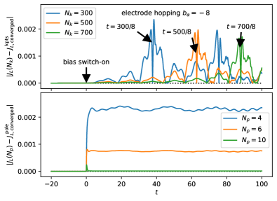
Figure 1: Transient currents at the left electrode interface in the dimer case compared to the converged results shown in Fig. 2 of main text. Top: $k$-points spectral decomposition with varying number of points $N_{k}$. Bottom: pole-expansion with varying number of poles $N_{p}$.

In Fig. 1, we show a calculation corresponding to the dimer system studied in Fig. 2 of the main text. The system is coupled to one-dimensional tight-binding electrodes (on-site energy $a_{\alpha}=\mu$, hopping $b_{\alpha}$) with the energy dispersion $\epsilon_{k\alpha}=a_{\alpha}-2|b_{\alpha}|\cos[\pi k/(N_{k}+1)]$ and the tunneling matrix elements (to terminal sites of the electrodes) $T_{ik\alpha}=T_{\alpha}\sqrt{2/(N_{k}+1)}\sin(\pi k/(N_{k}+1))$, where $N_{k}$ is the number of discretized $k$ points. Here, the left-interface current, evaluated for different numbers of the $k$ points ($N_{k}$) or poles ($N_{p}$) is compared to the converged result shown in the main text. We see that a recurrence time due to a finite-size effect is present in the spectral decomposition scheme. This recurrence time is equal to $N_{k}/|b_{\alpha}|$ and it corresponds to the time it takes for the electronic wavefront to go from one of the interfaces to the boundary of the corresponding electrode and back. Other limitations of the spectral decomposition scheme are discussed in the main text. In contrast, the pole expansion scheme shows no finite-size effects, but instead, if the number of poles is too low, the steady-value of the current is inaccurate. Compared to the spectral decomposition scheme, the pole expansion scheme converges extremely fast.

Within the temporal window of Fig. 2 in the main text and Fig. 1 above (up to $t=100$), the current has not yet reached a steady value. By evolving longer in time, however, a well defined steady state is attained. In Fig. 2 we show the results of a longer time evolution (up to $t=2000$); the current saturation is clearly visible. For this long-time evolution, a significantly higher number of $k$-points is required to reach converged results, in contrast to the number of poles which is instead the same.

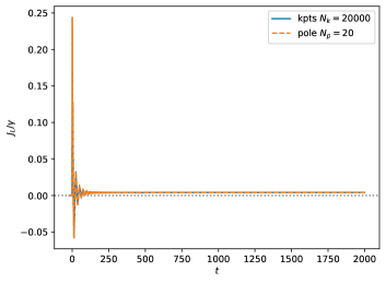
Figure 2: Long-time behaviour corresponding to Fig. 2(b) of the main text using the spectral-decomposition scheme and the pole expansion of the Fermi function.

VII Meir-Wingreen formula

The current between the system and the $\alpha$-th electrode can be calculated from the Meir-Wingreen formula, which consists of the $\alpha$-th electrode contribution to the embedding integral, cf. Eq. (IV):

$$J_{\alpha}(t)=2\mathrm{Re}\mathrm{Tr}I_{\alpha}(t)$$

$$=2\mathrm{Re}\mathrm{Tr}\left[\frac{1}{2}\Gamma_{\alpha}s_{\alpha}(t)\rho(t)-\frac{1}{4}\Gamma_{\alpha}s_{\alpha}(t)-\sum_{l}s_{\alpha}(t)\frac{\eta_{l}}{\beta}\Gamma_{\alpha}\mathcal{G}_{l\alpha}^{\text{em}}(t)\right]$$

$$=2s_{\alpha}(t)\mathrm{Re}\mathrm{Tr}\left[\Gamma_{\alpha}\left(\frac{2\rho(t)-1}{4}-{\sum_{l}}\frac{\eta_{l}}{\beta}G_{l\alpha}^{\text{em}}(t)\right)\right],$$ (28)

where the trace also contains a sum over spin.

Alternatively, the Meir-Wingreen formula can be cast in terms of the $k$-resolved embedding correlator:

$$J_{\alpha}(t)=2\mathrm{Re}\sum_{ik}T_{ik\alpha}s_{\alpha}(t)\widetilde{\mathcal{G}}_{k\alpha i}^{\text{em}}(t).$$ (29)

Remarkably, calculating the time-dependent current adds no extra complexity in either cases. The current formula is completely specified in terms of the single-time embedding correlator, which is readily available when evolving the coupled system of ODEs. With the pole expansion, this corresponds to Eqs. (V) and (V), and with the $k$-resolved spectral decomposition, to the first equality of Eq. (V), and Eqs. (VI) and (27).