Weight Predictor Network with Feature Selection
for Small Sample Tabular Biomedical Data

Abstract

Tabular biomedical data is often high-dimensional but with a very small number of samples. Although recent work showed that well-regularised simple neural networks could outperform more sophisticated architectures on tabular data, they are still prone to overfitting on tiny datasets with many potentially irrelevant features. To combat these issues, we propose Weight Predictor Network with Feature Selection (WPFS) for learning neural networks from high-dimensional and small sample data by reducing the number of learnable parameters and simultaneously performing feature selection. In addition to the classification network, WPFS uses two small auxiliary networks that together output the weights of the first layer of the classification model. We evaluate on nine real-world biomedical datasets and demonstrate that WPFS outperforms other standard as well as more recent methods typically applied to tabular data. Furthermore, we investigate the proposed feature selection mechanism and show that it improves performance while providing useful insights into the learning task.

1 Introduction

The wide availability of high-throughput sequencing technologies has enabled the collection of high-dimensional biomedical data containing measurements of the entire genome. However, many clinical trials which collect such high-dimensional, typically tabular, data are carried out on small cohorts of patients due to the scarcity of available patients, prohibitive costs, or the risks associated with new medicines. Although using deep networks to analyse such feature-rich data promises to deliver personalised medicine, current methods tend to perform poorly when the number of features significantly exceeds the number of samples.

Recently, a large number of neural architectures have been developed for tabular data, taking inspiration from tree-based methods (Katzir, Elidan, and El-Yaniv 2020; Hazimeh et al. 2020; Popov, Morozov, and Babenko 2020; Yang, Morillo, and Hospedales 2018), including attention-based modules (Arık and Pfister 2021; Huang et al. 2020), explicitly performing feature selection (Yang, Lindenbaum, and Kluger 2022; Lemhadri, Ruan, and Tibshirani 2021; Yoon, Jordon, and van der Schaar 2018), or modelling multiplicative feature interactions (Qin et al. 2021). However, such specialised neural architectures are not necessarily superior to tree-based ensembles (such as gradient boosting decision trees) on tabular data, and their relative performance can vary greatly between datasets (Gorishniy et al. 2021).

On tabular data, specialised neural architectures are outperformed by well-regularised feed-forward networks such as MLPs (Kadra et al. 2021). As such, we believe that designing regularisation mechanisms for MLPs holds great potential for improving performance on high-dimensional, small size tabular datasets.

Method	Data Type1	End-to-end	Feature	Additional	Additional Training	Feature	Differentiable
		Training	Selection	Decoder	Hyper-parameters	Embedding	Loss
DietNetworks	Discrete	✓	$\times$	✓	1	Histogram	✓
FsNet	Cont.	✓	✓	✓	2	Histogram	✓
CAE	Cont.	✓	✓	$\times$	1	-	✓
LassoNet	Cont.	✓	✓	$\times$	2	-	$\times$
DNP	Cont.	$\times$	✓	$\times$	1	-	✓
SPINN	Cont.	✓	✓	$\times$	4	-	$\times$
WPFS (ours)	Cont.	✓	✓	$\times$	1	Matrix factor.	✓

Table 1: Comparison with Related Work. ¹Denotes the most general regime under which each method is appropriate, but note that all methods for continuous data also support discrete data.

An important characteristic of feed-forward neural networks applied to high-dimensional data is that the first hidden layer contains a disproportionate number of parameters compared to the other layers. For example, on a typical genomics dataset with $\sim{20,\!000}$ features, a five-layer MLP with $100$ neurons per layer contains $98\%$ of the parameters in the first layer. We hypothesise that having a large learning capacity in the first layer contributes overfitting of neural networks on high-dimensional, small sample datasets.

In this paper, we propose Weight Predictor Network with Feature Selection (WPFS), a simple but effective method to overcome overfitting on high-dimensional, small sample tabular supervised tasks. Our method uses two tiny auxiliary networks to perform global feature selection and compute the weights of the first hidden layer of a classification network. Our method is generalisable and can be applied to any neural network in which the first hidden layer is linear. More specifically, our contributions include:

1. A novel method to substantially reduce the number of parameters in feed-forward neural networks and simultaneously perform global feature selection (Sec. 3). Our method extends DietNetworks to support continuous data, use factorised feature embeddings, perform feature selection, and it consistently improves performance.

2. A novel global feature selection mechanism that ranks features during training based on feature embeddings (Sec. 3). We propose a simple and differentiable auxiliary loss to select a small subset of features (Sec. 3.4). We investigate the proposed mechanisms and show that they improve performance (Sec. 4.2) and provide insights into the difficulty of the learning task (Sec. 4.5).

3. We evaluate WPFS on $9$ high-dimensional, small sample biomedical datasets and demonstrate that it performs better overall than $10$ methods including TabNet, DietNetworks, FsNet, CAE, MLPs, Random Forest, and Gradient Boosted Trees (Sec. 4.3). We attribute the success of WPFS to its ability to reduce overfitting (Sec. 4.4).

2 Related Work

We focus on learning problems from tabular datasets where the number of features substantially exceeds the number of samples. As such, this work relates to DietNetworks (Romero et al. 2017), which uses auxiliary networks to predict the weights of the first layer of an underlying feed-forward network (referred to as “fat layer”). FsNet (Singh et al. 2020) extends DietNetworks by combining them with Concrete autoencoders (CAE) (Balin, Abid, and Zou 2019). DietNetworks and FsNet use histogram feature embeddings, which are well-suited for discrete data, and require a decoder (with an additional reconstruction loss) to alleviate training instabilities. These mechanisms do not translate well to continuous-data problems (Sec.  4.1). In contrast, our WPFS takes matrix-factorised feature embeddings and uses a Sparsity Network for global feature selection, which help alleviate training instabilities, remove the need for an additional decoder network, and improve performance (Sec. 4.4). Table 1 further highlights the key differences between WPFS and the discussed related methods.

When learning from small sample tabular datasets, various neural architectures use a regularisation mechanism, such as $L_{1}$ (Tibshirani 1996) for performing feature selection. However, optimising $L_{1}$-constrained problems in parameter-rich neural networks may lead to local sub-optima (Bach 2017). To combat this, Liu et al. (2017) propose DNPs which employ a greedy approximation of $L_{1}$ focusing on individual features. In a similar context, SPINN (Feng and Simon 2017) employ a sparse group lasso regularisation (Simon et al. 2013) on the first layer. LassoNet (Lemhadri, Ruan, and Tibshirani 2021) combines a linear model (with $L_{1}$ regularisation) with a non-linear neural network to perform feature selection. These methods, however, typically require lengthy training procedures; be it retraining the model multiple times (DNP), using specialised optimisers (LassoNet, SPINN), or costly hyper-parameter optimisation (LassoNet, SPINN). All of these may lead to unfavourable properties when learning from high-dimensional, small size datasets.

In a broader context, approaches to reducing the number of learnable parameters have primarily addressed image-data problems rather than tabular data. Hypernetworks (Ha, Dai, and Le 2017) use an external network to generate the entire weight matrix for each layer of a classification network. However, the first layer is very large on high-dimensional tabular data and requires using large Hypernetworks. Also, Hypernetworks learn an embedding per layer, which can overfit on small size datasets. In contrast, our WPFS computes the weight matrix column-by-column from unsupervised feature embeddings.

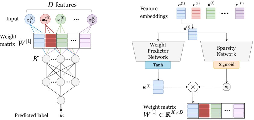
Figure 1: Architecture of the proposed Weight Predictor Network with Feature Selection (WPFS). (Left) A standard feed-forward neural network, highlighting the weight matrix ${\bm{W}}^{[1]}\in{\mathbb{R}}^{K\times D}$ of the first layer. (Right) We compute feature embeddings ${\bm{e}}^{(j)}$ for each feature $j$. WPFS uses two auxiliary networks to compute ${\bm{W}}^{[1]}$. First, the Weight Predictor Network (WPN) maps each feature embedding ${\bm{e}}^{(j)}$ to a vector ${\bm{w}}^{(j)}$. The Sparsity Network (SPN) maps the same feature embeddings ${\bm{e}}^{(j)}$ to scalars $s_{j}\in(0,1)$. The two outputs are multiplied ${\bm{w}}^{(j)}\cdot s_{j}$, and the result acts as the $j$-th column of ${\bm{W}}^{[1]}$. An element ${\bm{W}}^{[1]}_{k,j}$ represents the weight between feature $j$ and the neuron $k$ from the first layer. All three networks are trained simultaneously.

3 Method

3.1 Problem Formulation and Notation

We consider the problem setting of classification in ${\mathcal{Y}}$ classes. Let $\{({\bm{x}}^{(i)},y_{i})\}_{i=1}^{N}$ be a $D$-dimensional dataset of $N$ samples, where ${\bm{x}}^{(i)}\in{\mathbb{R}}^{D}$ (continuous) is a sample and $y_{i}\in{\mathcal{Y}}$ (categorical) is its label. The $j$-th feature of the $i$-th sample is represented as ${\bm{x}}^{(i)}_{j}$. We define the data matrix as ${\bm{X}}:=[{\bm{x}}^{(1)},...,{\bm{x}}^{(N)}]^{\top}\in{\mathbb{R}}^{N\times D}$, and the labels as ${\bm{y}}:=[y_{1},...,y_{N}]$. For each feature $j$ we consider having an embedding ${\bm{e}}^{(j)}\in{\mathbb{R}}^{M}$ of size $M$ (Sections 3.3, 4.1 explain and analyse multiple embedding types).

Let $f_{{\bm{W}}}:{\mathbb{R}}^{D}\rightarrow{\mathcal{Y}}$ denote a classification neural network with parameters ${\bm{W}}$, which inputs a sample ${\bm{x}}^{(i)}$ and outputs a predicted label $\hat{y}_{i}$. In this paper we consider only the class of neural network in which the first layer is linear. Let the first layer have size $K$ and define ${\bm{W}}^{[1]}\in{\mathbb{R}}^{K\times D}$ to be its weight matrix.

3.2 Model

We propose WPFS as an approach for generating the weights of the first layer in a neural network. Instead of learning ${\bm{W}}^{[1]}$ directly, WPFS uses two small auxiliary networks to compute ${\bm{W}}^{[1]}$ column-by-column (Figure 1). We want to bypass learning ${\bm{W}}^{[1]}$ directly because on high-dimensional tasks it contains over $95\%$ of the model’s learnable parameters, which increases the risk of overfitting. In practice, the proposed method reduces the total number of learnable parameters by $\sim 90\%$.

Next, we describe the two auxiliary networks. The pseudocode is summarised in Algorithm 1.

The Weight Predictor Network (WPN) $f_{{\bm{\theta}}_{\text{WPN}}}:{\mathbb{R}}^{M}\rightarrow{\mathbb{R}}^{K}$, with learnable parameters ${\bm{\theta}}_{\text{WPN}}$, maps a feature embedding ${\bm{e}}^{(j)}$ to a vector ${\bm{w}}^{(j)}\in{\mathbb{R}}^{K}$. Intuitively, for every feature $j$, the WPN outputs the weights ${\bm{w}}^{(j)}$ connecting feature $j$ with all $K$ neurons in the first hidden layer. All outputs are concatenated horizontally in the matrix ${\bm{W}}_{\text{WPN}}:=[{\bm{w}}^{(1)},...,{\bm{w}}^{(D)}]\in{\mathbb{R}}^{K\times D}$. We implement WPN as a $4$-layer MLP with a $tanh$ activation in the last layer.

The Sparsity Network (SPN) $f_{{\bm{\theta}}_{\text{SPN}}}:{\mathbb{R}}^{M}\rightarrow{\mathbb{R}}$, with learnable parameters ${\bm{\theta}}_{\text{SPN}}$, approximates the global feature importance scores. For every feature $j$, the SPN maps a feature embedding ${\bm{e}}^{(j)}$ to a scalar $s_{j}\in(0,1)$ which represents the global feature importance score of feature $j$. A feature has maximal importance if $s_{j}\rightarrow 1$, and can be dropped if $s_{j}\rightarrow 0$. All outputs are stored into a vector ${\bm{s}}:=[s_{1},...,s_{D}]\in{\mathbb{R}}^{D}$. We implement SPN as a $4$-layer MLP with a $sigmoid$ activation in the last layer.

The outputs of WPN and SPN are combined to compute the weight matrix of first linear layer of the classification model as ${\bm{W}}^{[1]}:=[{\bm{w}}^{(1)}\cdot s_{1},...,{\bm{w}}^{(D)}\cdot s_{D}]={\bm{W}}^{[1]}_{\text{WPN}}\operatorname{diag}({\bm{s}})$ (where $\operatorname{diag}({\bm{s}})$ is a square diagonal matrix with the vector ${\bm{s}}$ on the main diagonal). The last equation provides two justifications for the SPN.

On the one hand, the SPN can be interpreted as performing global feature selection. Passing an input ${\bm{x}}$ through the first layer is equivalent to ${\bm{W}}^{[1]}{\bm{x}}={\bm{W}}^{[1]}_{\text{WPN}}\operatorname{diag}({\bm{s}}){\bm{x}}={\bm{W}}^{[1]}_{\text{WPN}}(\operatorname{diag}({\bm{s}}){\bm{x}})={\bm{W}}^{[1]}_{\text{WPN}}({\bm{s}}\odot{\bm{x}})$ (where $\odot$ is the element-wise multiplication, also called the Hadamard product). The last equation illustrates that the feature importance scores ${\bm{s}}$ act as a ‘mask’ applied to the input ${\bm{x}}$. A feature $j$ is ignored when $s_{j}\rightarrow 0$. In practice, SPN learns to ignore most features (see Sec. 4.5).

On the other hand, the SPN can be viewed as rescaling ${\bm{W}}^{[1]}$ because each feature importance score $s_{j}$ scales column $j$ of the matrix ${\bm{W}}^{[1]}$. This interpretation solves a major limitation of DietNetwork, which uses a $tanh$ activation to compute the weights, and in practice, $tanh$ usually saturates and outputs large values $\in\{-1,1\}$. Note that SPN enables learning weights with small magnitudes, as is commonly used in successful weight initialisation schemes (Glorot and Bengio 2010; He et al. 2015).

3.3 Feature Embeddings

We investigate four methods to obtain feature embeddings ${\bm{e}}^{()}$, which serve as input to the auxiliary networks (WPN and SPN). We assume no access to external data or feature embeddings because we want to simulate real-world medical scenarios in which feature embeddings are usually unavailable. Previous work (Romero et al. 2017) showed that learning feature embeddings using end-to-end training, denoising autoencoders, or random projection may not be effective on small datasets, and we do not consider such embeddings.

We consider only unsupervised methods for computing feature embeddings because of the high risk of overfitting on supervised tasks with small training datasets:

1. Dot-histogram (Singh et al. 2020) embeds the shape and range of the distribution of the measurements for a feature. For every feature $j$, it computes the normalised histogram of the feature value ${\bm{X}}_{:,j}$. If we consider ${\bm{h}}^{(j)},{\bm{c}}^{(j)}$ to represent the heights and the centers of the histogram’s bins, the dot-histogram embedding is the element-wise product ${\bm{e}}^{(j)}:={\bm{h}}^{(j)}\odot{\bm{c}}^{(j)}$.

2. ‘Feature-values’ defines the embedding ${\bm{e}}^{(j)}:={\bm{X}}_{:,j}$ (i.e., ${\bm{e}}^{(j)}$ contains the measurements for feature $j$). This relatively simple embedding uses the scarcity of training samples to its advantage by preserving all information.

3. Singular value decomposition (SVD) has been used to compare genes expressions across different arrays (Alter, Brown, and Botstein 2000). It factorises the data matrix ${\bm{X}}=\text{eigengenes}\times\text{eigenarrays}$, where the “eigengenes” define an orthogonal space of representative gene prototypes and the “eigenarrays” represent the coordinates of each gene in this space. An embedding ${\bm{e}}^{(j)}$ is the $j$-th column of the “eigenarrays” matrix.

4. Non-negative matrix factorisation (NMF) has been applied in bioinformatics to cluster gene expression (Kim and Park 2007; Taslaman and Nilsson 2012) and identify common cancer mutations (Alexandrov et al. 2013). It approximates ${\bm{X}}\approx{\bm{W}}{\bm{H}}$, with the intuition that the column space of ${\bm{W}}$ represents “eigengenes”, and the column ${\bm{H}}_{:,j}$ represents coordinates of gene $j$ in the space spanned by the eigengenes. The feature embedding is ${\bm{e}}^{(j)}:={\bm{H}}_{:,j}$.

We found that the data matrix ${\bm{X}}$ must be preprocessed using min-max scaling in $[0,1]$ before computing the embeddings (Appx. B.1). We analyse the performance of each embedding type in Section 4.1.

Algorithm 1 Training the proposed method WPFS

Input: training data ${\bm{X}}\in{\mathbb{R}}^{N\times D}$, training labels ${\bm{y}}\in{\mathbb{R}}^{N}$, classification network $f_{{\bm{W}}}$, weight predictor network $f_{\theta_{\text{WPN}}}$, sparsity network $f_{\theta_{\text{SPN}}}$, sparsity loss hyper-parameter $\lambda$, learning rate $\alpha$

  Compute global feature embeddings:    ${\bm{e}}^{(1)},{\bm{e}}^{(2)},...,{\bm{e}}^{(D)}$ from ${\bm{X}}$

  for each minibatch $B=\{({\bm{x}}^{(i)},y_{i})\}_{i=1}^{b}$  do

     for each feature $j=1,2,...,D$  do

        ${\bm{w}}^{(j)}=f_{\theta_{\text{WPN}}}({\bm{e}}^{(j)})$ {Pass feature embedding through the WPN}

        $s_{j}=f_{\theta_{\text{SPN}}}({\bm{e}}^{(j)})$ {Pass feature embedding through the SPN}

        ${\bm{w}}^{(j)}={\bm{w}}^{(j)}\cdot s_{j}$

     end for

     Let ${\bm{W}}^{[1]}$ to be the matrix $\in{\mathbb{R}}^{K\times D}$ obtained by    horizontally concatenating ${\bm{w}}^{(1)},{\bm{w}}^{(2)},...,{\bm{w}}^{(D)}$

     Make ${\bm{W}}^{[1]}$ the weight matrix of the first layer of $f_{{\bm{W}}}$

     for each sample $i=1,2,...,b$ do

        $\hat{y}_{i}=f_{{\bm{W}}}({\bm{x}}^{(i)})$

     end for

     $\hat{{\bm{y}}}\leftarrow[\hat{y}_{1},\hat{y}_{2},...,\hat{y}_{b}]$ {Concatenate all predictions}

     Compute the training loss $L$:   $L=CrossEntropyLoss({\bm{y}},\hat{{\bm{y}}})+\lambda\cdot(s_{1}+s_{2}+...+s_{D})$

     Compute the gradient of the loss $L$ w.r.t.:    ${\bm{W}},\theta_{\text{WPN}},\theta_{\text{SPN}}$ using backpropagation

     Update the parameters:    ${\bm{W}}\leftarrow{\bm{W}}-\alpha\nabla_{{\bm{W}}}L,$   $\theta_{\text{WPN}}\leftarrow\theta_{\text{WPN}}-\alpha\nabla_{\theta_{\text{WPN}}}L,$   $\theta_{\text{SPN}}\leftarrow\theta_{\text{SPN}}-\alpha\nabla_{\theta_{\text{SPN}}}L$

  end for

Return: Trained models $f_{{\bm{W}}},f_{\theta_{\text{WPN}}},f_{\theta_{\text{SPN}}}$

3.4 Training Objective

The training objective is composed of the average cross-entropy loss and a simple sparsity loss. For each sample, the cross-entropy loss $\ell\left(f_{{\bm{W}}}({\bm{x}}^{(i)}),y_{i};f_{{\bm{\theta}}_{\text{WPN}}},f_{{\bm{\theta}}_{\text{SPN}}}\right)$ is computed between the label predicted using the classification network $f_{{\bm{W}}}({\bm{x}}^{(i)})$ and the true label $y_{i}$. Note that the auxiliary networks $f_{{\bm{\theta}}_{\text{WPN}}}$ and $f_{{\bm{\theta}}_{\text{SPN}}}$ are used to compute the weights of the first layer of the classifier $f_{{\bm{W}}}$ and this enables computing gradients for their parameters (${\bm{\theta}}_{\text{WPN}},{\bm{\theta}}_{\text{SPN}}$).

We define a differentiable sparsity loss to incentivise the classifier to use a small number of features. The sparsity loss is the sum of the SPN’s feature importance scores $s_{j}$ output. Note that $s_{j}>0$ because they are output from a sigmoid function. To provide intuition for our sparsity loss, we remark that it is a special case of the $L_{1}$ norm with all terms being strictly positive. Adding $L_{1}$ regularisation is effective in performing feature selection (Tibshirani 1996).

$$L({\bm{W}},{\bm{\theta}}_{\text{WPN}},{\bm{\theta}}_{\text{SPN}})=\frac{1}{N}\sum_{i=1}^{N}\ell\left(f_{{\bm{W}}}({\bm{x}}^{(i)}),y_{i};f_{{\bm{\theta}}_{\text{WPN}}},f_{{\bm{\theta}}_{\text{SPN}}}\right)+\lambda\sum_{j=1}^{D}f_{{\bm{\theta}}_{\text{SPN}}}({\bm{e}}^{(j)})$$ (1)

Optimisation.

As the loss is differentiable, we compute the gradients for the parameters of all three networks and use standard gradient-based optimisation algorithms (e.g., AdamW). The three networks are trained simultaneously end-to-end to minimise the objective function. We did not observe optimisation issues by training over $10000$ models.

4 Experiments

In this section, we evaluate our method for classification tasks and substantiate the proposed architectural choices. Through a series of experiments, we analyse multiple feature embedding types (Sec. 4.1), the impact of the auxiliary Sparsity Network on the overall performance of WPFS, and its ability to perform feature selection (Sec. sec:influence-spn-performance). We then compare the performance of WPFS against the performance of several common methods (Sec. 4.3) and analyse the training behaviour of WPFS (Sec.  4.4). Lastly, we showcase how the SPN can provide insights into the learning task (Sec. 4.5).

Datasets.

We focus on high-dimensional, small size datasets and consider $9$ real-world tabular biomedical datasets with continuous values. The datasets contain $3312-19993$ features, and between $100-200$ samples. The number of classes ranges between $2-4$. Appx. A.1 presents complete details about the datasets.

Setup and evaluation.

For each dataset, we perform $5$-fold cross-validation repeated $5$ times, resulting in $25$ runs per model. We randomly select $10\%$ of the training data for validation for each fold. We purposely constrain the size of the datasets (even for larger ones) to simulate real-world practical scenarios with small size datasets. For training all methods, we use a weighted loss (e.g., weighted cross-entropy loss for all neural networks). For each method, we perform a hyper-parameter search and choose the optimal hyper-parameters based on the performance of the validation set. We perform model selection using the validation cross-entropy loss. Finally, we report the balanced accuracy of the test set, averaged across all $25$ runs. Appx. A contains details on reproducibility and hyper-parameter tuning.

WPFS settings.

The classification network is a $3$-layer feed-forward neural network with $100,100,10$ neurons and a softmax activation in the last layer. The auxiliary WPN and SPN networks are $4$-layer feed-forward neural networks with $100$ neurons. WPN has a $tanh$ activation in the last layer, and SPN has a $sigmoid$ activation. All networks use batch normalisation (Ioffe and Szegedy 2015), dropout (Srivastava et al. 2014) with $p=0.2$ and LeakyReLU nonlinearity internally. We train with a batch size of $8$ and optimise using AdamW (Loshchilov and Hutter 2019) with a learning rate $3e-3$ and weight decay of $1e-4$. We use a learning-rate scheduler, linearly decaying the learning rate from $3e-3$ to $3e-4$ over $500$ epochs, and continue training with $3e-4$ .

Dataset	WPFS (ours)	DietNets	FsNet	CAE	LassoNet	DNP	SPINN	TabNet	MLP	RF	LGBM
cll	79.14	68.84	66.38	71.94	30.63	85.12	85.34	57.81	78.30	82.06	85.59
lung	94.83	90.43	91.75	85.00	25.11	92.83	92.26	77.65	94.20	91.81	93.42
metabric-dr	59.05	56.98	56.92	57.35	48.88	55.79	56.13	49.18	59.56	51.38	58.23
metabric-pam50	95.96	95.02	83.86	95.78	48.41	93.56	93.56	83.60	94.31	89.11	94.97
prostate	89.15	81.71	84.74	87.60	54.78	90.25	89.27	65.66	88.76	90.78	91.38
smk	66.89	62.71	56.27	59.96	51.04	66.89	68.43	54.57	64.42	68.16	65.70
tcga-2ysurvival	59.54	53.62	53.83	59.54	46.08	58.13	57.70	51.58	56.28	61.30	57.08
tcga-tumor-grade	55.91	46.69	45.94	40.69	33.49	44.71	44.28	39.34	48.19	50.93	49.11
toxicity	88.29	82.13	60.26	60.36	26.67	93.5	93.5	40.06	93.21	80.75	82.40
Average rank	2.66	6.66	7.88	6.22	11	4.33	4.33	10	4.44	4.55	3.44

Table 2: Evaluation of WPFS and $8$ baselines methods on $9$ biomedical datasets. We report the balanced accuracy averaged over $25$ runs. On each dataset, we rank the methods based on their performance. We compute the average rank of each method across datasets (a smaller rank implies higher performance). WPFS ranks the best across all methods.

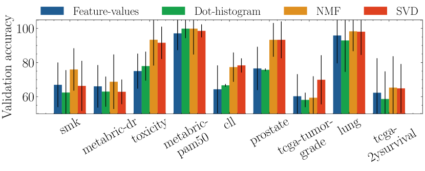
Figure 2: Comparing the validation performance of WPFS with four feature embedding types. We report the mean and standard deviation of the balanced accuracy, averaged across data splits. Across $9$ datasets, feature embeddings based on matrix factorisation (SVD and NMF) outperform ‘feature-values’ and ‘dot-histogram’ embeddings.

4.1 Impact of the Feature Embedding Type

We start by investigating the impact of the feature embedding type on the model’s performance. We use and report the validation performance (rather than test performance) not to overfit the test data. The two auxiliary networks take as input feature embeddings to compute the weights of the classifier’s first layer ${\bm{W}}^{[1]}$. Different approaches exist for preprocessing the data ${\bm{X}}$ before computing the embeddings. We found that $[0,1]$ scaling leads to better and more stable results than using the raw data or performing Z-score normalisation (Appx. B presents extended results).

We evaluate the classification performance using four embedding types. In this experiment, we fix the size of the embedding to $50$ and remove the SPN network so that ${\bm{W}}^{[1]}={\bm{W}}_{\text{WPN}}$. In principle, dropping the SPN and using the dot-histogram is a close adaptation of DietNetworks to continuous data, and it allows us to evaluate our statements in Section 2 that the embedding type affects the performance.

In general, we found that using NMF embeddings leads to more stable and accurate performance (Figure 2). In all except one case, the performance of the NMF embeddings is better or on-par with the SVD embeddings, with both exhibiting substantially better performance than dot-histogram and feature-values. In most cases, the “simple” feature-values embedding outperforms the dot-histogram embeddings. We believe dot-histogram cannot represent continuous data accurately because the choice of bins can be highly impacted by the outliers and the noise in the data. We use NMF embeddings in all subsequent sections.

We also investigated the influence of the size of the embeddings on the performance. We found that in most cases, an embedding of size $50$ led to optimal results, with optimal sizes for ‘lung’ and ‘cll’ being $20$ and $70$, respectively (Appx. B contains extended results of this analysis).

4.2 Impact of the Feature Selection Mechanisms

Next, we analyse how the auxiliary SPN impacts the overall performance. To isolate the effect of the SPN, we remove the sparsity loss (i.e., set $\lambda=0$) and train and evaluate two identical setups: one with and one without the auxiliary SPN. Figure 3 shows the improvement in test accuracy (Appx. C presents extended results). In all cases, adding the SPN network leads to better performance. While these improvements vary from one dataset to another, the results show that the SPN is an appropriate regularisation mechanism and reduces potential unwanted saturations of the WPN .

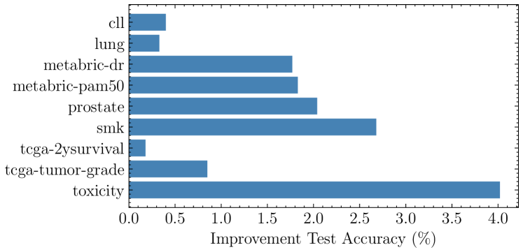
Figure 3: The effect of SPN on the WPFS performance. We report the average test accuracy improvement of a WPFS which includes a SPN over an identical WPFS without SPN. We trained without the sparsity loss ($\lambda=0$) to isolate SPN’s effect. Adding the SPN always improves the performance.

Recall that WPFS can be trained using an additional sparsity loss computed from the output ${\bm{s}}$ of the SPN. We study the effect of the sparsity loss by training the complete WPFS model (including the WPN and SPN) and varying the hyper-parameter $\lambda$ which controls the magnitude of the sparsity loss. We observe that the sparsity loss increases the performance of WPFS on $8$ out of $9$ datasets (Appx. 9 contains the ablation on $\lambda$). In general, $\lambda=3e-5$ leads to the best performance improvement, but choosing $\lambda$ is still data-dependent and it should be tuned. We suggest trying values for $\lambda$ such that the ratio between the cross-entropy loss and the sparsity loss is $\{0.05,0.1,0.2,0.5,1\}$.

4.3 Classification Performance of WPFS

Having investigated the individual impact of the proposed architectural choices, we proceed to evaluate the test performance of WPFS against a version of DietNetworks adapted for continuous data by using the dot-histogram embeddings presented in Section 3.3. We compare to methods mentioned in Related Works, including FsNet, CAE, LassoNet, SPINN and DNP. We also compare to standard methods such as TabNet (Arık and Pfister 2021), Random Forest (RF) (Breiman 2001), LightGBM (LGBM) (Ke et al. 2017) and an MLP. We report the mean balanced test accuracy, and include the standard deviations in Appx. G.

WPFS exhibits better or comparable performance than the other benchmark models (Table 2). Specifically, we computed the average rank of each model’s performance across tasks and found that WPFS ranks best, followed by tree-based ensembles (LightGBM and Random Forest) and neural networks performing feature sparsity using $L_{1}$ (SPINN, DNP). Note that WPFS consistently outperformed other ‘parameter-efficient’ models such as DietNetworks and FsNet. We also found that complex and parameter-heavy architectures such as TabNet, CAE and LassoNet struggle in these scenarios and are surpassed by simple but well-regularised MLPs, which aligns with the literature (Kadra et al. 2021).

In most cases, WPFS is able to perform substantially better than MLPs, struggling only in the case of ‘toxicity’. As the MLP is already well-regularised, we attribute the performance improvement of WPFS to its ability to reduce the number of learnable parameters and therefore overcome severe overfitting, typical for such small size data problems.

4.4 Training Behaviour

Figure 4: Train and validation loss curves for an MLP and WPFS with an identical architecture for the classification network, on ‘lung’ and ‘tcga-tumor-grade’ datasets. The MLP shows high overfitting, as the validation loss quickly diverges while the training loss converges. WPFS’s validation loss decreases for longer and achieves better minima.

Since WPFSs are able to outperform other neural networks, we attribute this to the additional regularisation capabilities of the WPN and SPN networks. To investigate this hypothesis, we analysed the trends of the train/validation loss curves of WPFS (with WPN and SPN) and MLP. Figure 4 shows the train and validation loss curves for training on ‘lung’ and ‘tcga-tumor-grade’ datasets (see Appx. I for extended results for all datasets). Although the training loss consistently decreases for both models, there is a pronounced difference in the validation loss convergence. Specifically, the validation loss of the MLP diverges quickly and substantially from the training loss, indicating overfitting. In contrast, the WPFS validation loss indicates less overfitting because it decreases for longer and achieves a lower minimum than the MLP. The disparities in convergence translate into the test results from Table 2, where WPFS outperforms the MLP. We also found that using the WPN in our model leads to performance improvment in all but two cases (‘cll’ and ‘toxicity’), when its addition renders subpar but comparable performance to an MLP (see Appx. D).

WPFS exhibit stable performance, as indicated by the average standard deviation of the test accuracy across datasets (Appx. G). This is consistent when varying the sample size, with WPFSs outperforming MLPs on smaller datasets, with the latter closing the performance gap as sample size increases (see Appx. F).

Note, however, that these results are obtained using $10\%$ of the training data for validation, which translates into only a handful of samples for such small size datasets. While having small validation sets is not ideal and greatly influences model selection (evident from the instabilities in the validation loss curves), we purposely constrained the experimental setting to mimic a real-world practical scenario. Therefore, obtaining stable validation loss and performing model selection remains an open challenge.

4.5 Feature Importance and Interpretability

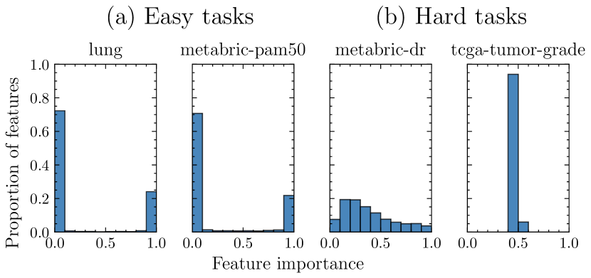
Figure 5: The distribution of the feature importance scores computed by WPFS provides insights into the difficulty of the learning task. WPFS assigns almost binary feature importance scores for ‘easy’ tasks while it struggles to make a ‘clear-cut’ of the important features on ‘hard’ tasks.

In Section 4.2 we showed that the proposed feature selection mechanism consistently improves the performance. In our final set of analyses, we seek qualitative insights into the feature selection mechanism.

Firstly, we examine how varying the sparsity loss impacts the WPFS’s ability to determine the important features. Let’s consider a feature $j$ is being selected when the score $s_{j}>0.95$, and not selected when $s_{j}<0.95$. Figure 6 shows the proportion of selected features while varying the sparsity hyper-parameter $\lambda$. Notice that, across datasets, WPFS selects merely $\sim 25\%$ of features without being trained with the sparsity loss (i.e., $\lambda=0$), which we believe is due to using a sigmoid activation for SPN. By increasing $\lambda$, the proportion of selection features decreases to $\sim 0.1-1\%$. In Appx. H) we show that increasing $\lambda$ changes the distribution of feature importance scores in a predictable manner. Although we expected these outcomes, we believe they are essential properties of WPFS, which can enable interpretable post-hoc analyses of the results.

Lastly, we discovered that the feature importance scores ${\bm{s}}$ computed by WPFS give insight into the task’s difficulty. We denote a task as ‘easy’ when WPFS obtains high accuracy and ‘hard’ when WPFS obtains low accuracy. In this experiment, we analysed the performance of WPFS without sparsity loss (by setting $\lambda=0$). On easy tasks (Fig. 5 (a)), we observe that WPFS has high certainty and assigns almost binary $\in\{0,1\}$ feature importance scores, with a negligible proportion of features in between. In contrast, on hard tasks (Fig. 5 (b)), the model behaves conservatively, and it cannot rank the features with certainty (this is most evident on ‘tcga-tumor-grade’, where WPFS assigns $0.5$ feature importance score to all features). This behaviour provides a built-in mechanism for debugging training issues, and analysing it from a domain-knowledge perspective may lead to further performance improvements. We conjecture that these findings link to WPFS’s ability to identify spurious correlations, and we leave this investigation for future work.

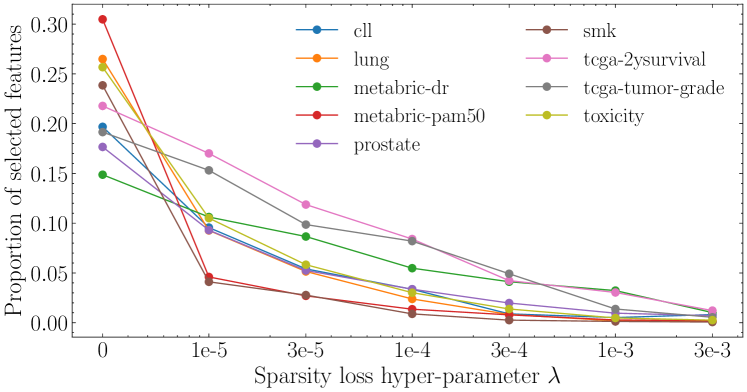
Figure 6: Proportion of selected features for different sparsity loss hyper-parameter $\lambda$, averaged across all runs. Increasing $\lambda$ reduces the proportion of selected features from $\sim 25\%$ to less than $1\%$, enabling post-hoc analyses of the selected features, possibly using domain knowledge.

5 Conclusion

We present Weight Predictor Network with Feature Selection (WPFS), a general method for learning from high-dimensional but extremely small size tabular data. Although well-regularised simple neural networks outperform more sophisticated architectures on tabular data, they are still prone to overfitting on very small datasets with many potentially irrelevant features. Motivated by this, we design an end-to-end method that combines a feed-forward network with two auxiliary networks: a Weight Predictor Network (WPN) that reduces the number of learnable parameters and a Sparsity Network (SPN) that performs feature selection and serves as an additional regularisation mechanism.

We investigated the capabilities of WPFS through a series of experiments on nine real-world biomedical datasets. We demonstrated that WPFS outperforms ten methods for tabular data while delivering the most stable classification accuracy. These results are encouraging, especially because neural networks typically struggle in this setting of high-dimensional, small size tabular datasets. We attribute the success of WPFS to its ability to reduce overfitting. We analysed the train-validation loss curves and showed that WPFS’s validation loss converges for longer and achieves better minima than an MLP. Lastly, we analysed the feature selection mechanism of WPFS and uncovered favourable properties, such as using only a small set of features that can be analysed, possibly using domain knowledge.

Supplementary Material for Submission “Weight Predictor Network with Feature Selection for Small Sample Tabular Biomedical Data”

Appendix A Reproducibility

A.1 Datasets

Table 3: Details of the 9 real-world biomedical datasets used for experiments. The number of features is 15-110 times larger than the number of samples.

Dataset	# Samples	# Features	# Classes	# Samples per class
cll	111	11340	3	11, 49, 51
lung	197	3312	4	17, 20, 21, 139
metabric-dr	200	4160	2	61, 139
metabric-pam50	200	4160	2	33, 167
prostate	102	5966	2	50, 52
smk	187	19993	2	90, 97
tcga-2ysurvival	200	4381	2	78, 122
tcga-tumor-grade	200	4381	3	25, 52, 124
toxicity	171	5748	4	39, 42, 45, 45

Table 3 summarises the datasets. Five datasets are open-source (Li et al. 2018) and available online (https://jundongl.github.io/scikit-feature/datasets.html): CLL-SUB-111 (called ‘cll’) (Haslinger et al. 2004), lung (Bhattacharjee et al. 2001), Prostate_GE (called ‘prostate’) (Singh et al. 2002), SMK-CAN-187 (called ‘smk’) (Spira et al. 2007) and TOX-171 (called ‘toxicity’) (Bajwa et al. 2016).

We derived two datasets from the METABRIC (Curtis et al. 2012) dataset. We combined the molecular data with the clinical label ‘DR’ to create the ‘metabric-dr’ dataset, and we combined the molecular data with the clinical label ‘Pam50Subtype’ to create the ‘metabric-pam50’ dataset. Because the label ‘Pam50Subtype’ was very imbalanced, we transformed the task into a binary task of basal vs non-basal by combining the classes ‘LumA’, ‘LumB’, ‘Her2’, ‘Normal’ into one class and using the remaining class ‘Basal’ as the second class. For both ‘metabric-dr’ and ‘metabric-pam50’ we selected the Hallmark gene set (Liberzon et al. 2015) associated with breast cancer, and the new datasets contain $4160$ expressions (features) for each patient. We created the final datasets by randomly sampling $200$ patients stratified because we are interested in studying datasets with a small sample size.

We derived two datasets from the TCGA (Tomczak, Czerwińska, and Wiznerowicz 2015) dataset. We combined the molecular data and the label ‘X2yr.RF.Surv’ to create the ‘tcga-2ysurvival’ dataset, and we combined the molecular data and the label ‘tumor_grade’ to create the ‘tcga-tumor-grade’ dataset. For both ‘tcga-2ysurvival’ and ‘tcga-tumor-grade’ we selected the Hallmark gene set (Liberzon et al. 2015) associated with breast cancer, leaving $4381$ expressions (features) for each patient. We created the final datasets by randomly sampling $200$ patients stratified because we are interested in studying datasets with a small sample size.

Dataset processing

Before training the models, we apply Z-score normalisation to each dataset. Specifically, on the training split, we learn a simple transformation to make each column of ${\bm{X}}_{train}\in{\mathbb{R}}^{N_{train}\times D}$ have zero mean and unit variance. We apply this transformation to the validation and test splits during cross-validation.

A.2 Computing Resources

We trained over $40,000$ models on a single machine from an internal cluster with a GPU Nvidia Quadro RTX 8000 with 48GB memory and an Intel(R) Xeon(R) Gold 5218 CPU @ 2.30GHz with 16 cores. The operating system was Ubuntu 20.04.4 LTS.

A.3 Training Details and Hyper-parameter Tuning

Software implementation.

All software dependencies, alongside their versions, are specified in the associated code. We implemented Random Forest using scikit-learn (Pedregosa et al. 2011), LightGBM using the lightgbm library (Ke et al. 2017) and TabNet (Arık and Pfister 2021) using a popular implementation from Dreamquark AI (www.github.com/dreamquark-ai/tabnet). We re-implemented FsNet (Singh et al. 2020) because the official code implementation contains differences from the paper, and they used a different evaluation setup from ours (they evaluated using unbalanced accuracy, while we run multiple data splits and evaluate using balanced accuracy). We used the official implementation of LassoNet (https://github.com/lasso-net/lassonet), and the official implementation of SPINN (https://github.com/jjfeng/spinn). We implemented MLP, DietNetworks, CAE our proposed WPFS in PyTorch (Paszke et al. 2019). We implemented NMF using a popular GPU-based NMF package (www.github.com/yoyololicon/pytorch-NMF).

Training details.

We present the most important training settings (all other implementation details are included in the associated codebase). The per-dataset hyper-parameters are discussed in the next paragraph and Table 4. We perform a fair comparison whenever possible. For example, use train all models using a weighted loss, evaluate using balanced accuracy, and use the same classification network architecture for WPFS, MLP, FsNet, CAE and DietNetworks.

• WPFS, DietNetworks, FsNet, CAE have three hidden layers of size $100,100,10$. The Weight Predictor Network and the Sparsity Network have four hidden layers $100,100,100,100$. They are trained for $10000$ iterations using early stopping with patience $200$ on the validation cross-entropy and gradient clipping at $2.5$. For CAE and FsNet we use the suggested annealing schedule for the concrete nodes: exponential annealing from temperature $10$ to $0.01$. On all datasets, DietNetworks performed best with not decoder.

• LassoNet has three hidden layers of size $100,100,10$. We use dropout $0.2$, and train using AdamW (with betas $0.9,0.98$) and a batch size of 8. We train using a weighted loss. We perform early stopping on the validation set.

• For Random Forest we used $500$ estimators, feature bagging with the square root of the number of features, and used balanced weights associated with the classes.

• For LightGBM we used $200$ estimators, feature bagging with $30\%$ of the features, a minimum of two instances in a leaf, and trained for $10000$ iterations to minimise the balanced cross-entropy. We perform early stopping on the validation set.

• For TabNet we use width 8 for the decision prediction layer and the attention embedding for each mask (larger values lead to severe overfitting), and $1.5$ for the coefficient for feature reusage in the masks. We use three steps in the architecture, with two independent and two shared Gated Linear Units layers at each step. We train using Adam with momentum $0.3$ and clip the gradients at $2$.

• For SPINN we used $\alpha=0.9$ for the group lasso in the sparse group lasso, the sparse group lasso hyper-parameter $\lambda=0.0032$, ridge-param $\lambda_{0}=0.0001$, and train for at most $1000$ iterations.

• For DNP we did not find any suitable implementation, and used SPINN with different settings as a proxy for DNP (because DNP is a greedy approximation to optimizing the group lasso, and SPINN optimises directly a group lasso). Specifically, our proxy for DNP results is SPINN with $\alpha=1$ for the group lasso in the sparse group lasso, the sparse group lasso hyper-parameter $\lambda=0.0032$, ridge-param $\lambda_{0}=0.0001$, and train for at most $1000$ iterations.

Table 4: Best performing hyper-parameters for each baseline and each dataset.

Dataset	Random Forest		LightGBM		TabNet		FsNet		CAE
	max	min samples	learning	max	learning	$\lambda$ sparsity	learning	$\lambda$	annealing
	depth	leaf	rate	depth	rate		rate	reconstruction	iterations
cll	3	3	0,1	2	0,03	0,001	0,003	0	1000
lung	3	2	0,1	1	0,02	0,1	0,001	0	1000
metabric-dr	7	2	0,1	1	0,03	0,1	0,003	0	300
metabric-pam50	7	2	0,01	2	0,02	0,001	0,003	0	1000
prostate	5	2	0,1	2	0,02	0,01	0,003	0	1000
smk	5	2	0,1	2	0,03	0,001	0,003	0	1000
tcga-2ysurvival	3	3	0,1	1	0,02	0,01	0,003	0	300
tcga-tumor-grade	3	3	0,1	1	0,02	0,01	0,003	0	300
toxicity	5	3	0,1	2	0,03	0,1	0,001	0,2	1000

Hyper-parameter tuning.

For each model, we used random search and previous experience to find a good range of hyper-parameter values that we could investigate in detail. After we found a good range for the hyper-parameters, we performed a grid-search and trained using 5-fold cross-validation with 5 repeats (training 25 models each run).

For the MLP and DietNetworks we individually grid-searched learning rate $\in\{0.003,0.001,0.0003,0.0001\}$, batch size $\in\{8,12,16,20,24,32\}$, dropout rate $\in\{0,0.1,0.2,0.3,0.4,0.5\}$. We found that learning rate $0.003$, batch size $8$ and dropout rate $0.2$ work well across datasets for both models, and we used them in the presented experiments. In addition, for DietNetworks we also tuned the reconstruction hyper-parameter $\lambda\in\{0,0.01,0.03,0.1,0.3,1,3,10,30\}$ and found that across dataset having $\lambda=0$ performed best. For WPFS we used the best hyper-parameters for the MLP and tuned only the sparsity hyper-parameter $\lambda\in\{0,3e-6,3e-5,3e-4,3e-3,1e-2\}$ (Appx. E) and the size of the feature embedding $\in\{20,50,70\}$ (Appx. B.2). For CAE we grid-search the learning rate in $\{0.0001,0.001\}$ and the number of annealing iterations in $\{300,1000\}$ (the models train for $\sim 1000-2000$ iterations with early stopping). For FsNet we grid-search the reconstruction parameter in $\lambda\in\{0,0.2,1,5\}$ and learning rate in $\{0.001,0.003\}$. For LightGBM we performed grid-search for the learning rate in $\{0.1,0.01\}$ and maximum depth in $\{1,2\}$. For Random Forest, we performed a grid search for the maximum depth in $\{3,5,7\}$ and the minimum number of samples in a leaf in $\{2,3\}$. For TabNet we searched the learning rate in $\{0.01,0.02,0.03\}$ and the $\lambda$ sparsity hyper-parameter in $\{0.1,0.01,0.001,0.0001\}$, as motivated by (Yang, Lindenbaum, and Kluger 2022). We selected the best hyper-parameters (Table 4) on the weighted cross-entropy (except Random Forest, for which we used weighted balanced accuracy).

LassoNet unstable training.

We used the official implementation of LassoNet (https://github.com/lasso-net/lassonet), and we successfully replicated some of the results in the LassoNet paper (Lemhadri, Ruan, and Tibshirani 2021). However, LassoNet was unstable on all the $9$ datasets we trained on. We included a Jupyter notebook in the attached codebase that demostrates that LassoNet cannot even fit the training data on our datasets.

In our experiments, we grid-searched the $L_{1}$ penalty coefficient $\lambda\in\{0.001,0.01,0.1,1,10,`auto^{\prime}\}$ and the hierarchy coefficient $M\in\{0.1,1,3,10\}$. These values are suggested in the paper and used in the examples from the official codebase. For all hyper-parameter combinations, LassoNet’s performance was equivalent to a random classifier (e.g., $25\%$ balanced accuracy for a $4$-class problem).

NMF.

We used standard NMF to compute a rank $k$ approximation ($k$ is mentioned in each experiment, but usually $k=50$) of the data matrix ${\bm{X}}\approx WH$, where $H\in{\mathbb{R}}^{k\times D}$. A column $H_{:i}$ represents the embedding for feature $i$. We trained the NMF for 1000 iterations to minimise the error under the Frobenius norm. We computed embeddings only on the training split and used the resulting embeddings also during validation and testing.

Appendix B Feature Embeddings

B.1 Ablation Data Preprocessing for Computing the Feature Embeddings

We investigate the impact of preprocessing the data matrix ${\bm{X}}$ before computing the embeddings. We consider three types of data preprocessing: min-max rescales the values of each feature in $[0,1]$, Z-score makes each feature have zero mean, and unit variance and raw does not apply any preprocessing to the data. We fix the size of the embedding to $50$ and remove the effect of the auxiliary SPN network (SPN always outputs ${\bm{s}}=1$, such that ${\bm{W}}^{[1]}={\bm{W}}^{[1]}_{WPN}$).

Tables 5 and 6 show the validation performance of WPFS on 9 datasets. We consider two types of preprocessing for each embedding type. Z-score normalisation cannot be applied for NMF because NMF requires the input to have all positive values. We find that NMF outperforms ‘feature-values’ and ‘dot-histogram’ by a large margin while being slightly better than SVD. We concluded that min-max preprocessing is most suitable for NMF because it scales the data into a consistent range, reducing the risk that the embeddings have large values. Figure 2 is created by plotting the results obtained with min-max preprocessing.

Table 5: Performance of WPFS using ‘feature-values’ and ‘dot-histogram’ feature embeddings. Before computing the embeddings, the data matrix ${\bm{X}}$ is preprocessed using ‘min-max’ or ‘Z-score’. We report the mean and standard deviation for the balanced accuracy on the validation split.

Embedding type	Feature-values		Dot-histogram
Preprocessing	min-max	Z-score	min-max	Z-score
cll	$64,33\pm 18,4$	$62\pm 15,79$	$66,67\pm 16,14$	$63,67\pm 15$
lung	$95,86\pm 7,2$	$95,82\pm 7,28$	$92,95\pm 9,45$	$90,36\pm 9,67$
metabric-dr	$66,07\pm 14$	$65,56\pm 13,17$	$62,98\pm 12,67$	$62,87\pm 14,81$
metabric-pam50	$97,08\pm 5,55$	$96,87\pm 6,97$	$99,85\pm 0,77$	$96,62\pm 6,11$
prostate	$76,56\pm 15,05$	$80,8\pm 17,95$	$75,76\pm 15,1$	$76,8\pm 11,89$
smk	$66,96\pm 13,05$	$67,54\pm 10,91$	$62,43\pm 12,45$	$65,18\pm 10,91$
tcga-2ysurvival	$62,33\pm 10,77$	$62,87\pm 11,47$	$58,67\pm 14,37$	$63,6\pm 13,6$
tcga-tumor-grade	$60,27\pm 12,59$	$63,53\pm 11,93$	$58,13\pm 11,58$	$59,47\pm 13,55$
toxicity	$75\pm 20,21$	$84,46\pm 11,38$	$77,92\pm 13,15$	$83,75\pm 13,77$
Average	$73,82\pm 12,98$	$75,49\pm 11,87$	$72,81\pm 11,74$	$73,59\pm 12,14$

Table 6: Performance of WPFS using Non-negative matrix factorisation (NMF) and Singular Value Decomposition (SVD) feature embeddings. Before computing the embeddings, the data matrix ${\bm{X}}$ is either not pre-processed (column ‘raw’) or preprocessed using ‘min-max’, ‘Z-score’. We report the mean and standard deviation for the balanced accuracy on the validation split.

Embedding type	NMF		SVD
Preprocessing	min-max	raw	min-max	Z-score
cll	$77,33\pm 12,39$	$80,33\pm 17,98$	$78,33\pm 15,96$	$77,67\pm 10,95$
lung	$98,27\pm 3,8$	$97,36\pm 5,05$	$98,05\pm 4,13$	$97,77\pm 4,66$
metabric-dr	$68,76\pm 12,93$	$67,67\pm 12,03$	$62,87\pm 16,29$	$65,89\pm 15,06$
metabric-pam50	$99,85\pm 0,77$	$99,54\pm 1,28$	$98,56\pm 4,22$	$98,87\pm 3,48$
prostate	$93,3\pm 8,56$	$92\pm 9,19$	$93,3\pm 9,86$	$95,2\pm 7,21$
smk	$75,96\pm 10,23$	$74,75\pm 11,59$	$66,32\pm 9,8$	$67\pm 10,65$
tcga-2ysurvival	$65,33\pm 13,58$	$60,27\pm 11,06$	$64,87\pm 14,31$	$63,13\pm 10,47$
tcga-tumor-grade	$59,4\pm 18,36$	$65\pm 14,38$	$69,93\pm 14,68$	$66,07\pm 12,71$
toxicity	$93,33\pm 8,82$	$93,83\pm 7,52$	$91,58\pm 8,46$	$93,42\pm 9,37$
Average	$81,28\pm 9,93$	$81,19\pm 10,00$	$80,42\pm 10,85$	$80,55\pm 9,39$

B.2 Ablation Feature Embedding Size

We investigate the robustness of WPFS to the size of the embedding. We train the WPFS model (with the two auxiliary networks) following the protocol presented in Section 4, but use a batch size of 16. We use NMF embeddings with min-max preprocessing and set the sparsity hyper-parameter $\lambda=0$.

Table 7 shows the validation weighted cross-entropy averaged across 25 runs. Varying the embedding size changes little the validation loss, and an embedding of size $50$ performs well across datasets. However, on some datasets WPFS performs better for different embedding sizes (e.g., on ‘lung’ dataset performs substantially better with a smaller embedding). We conclude that WPFS is robust to the choice of the embedding size, and, from a practical perspective, we suggest using an embedding of size $50$ in the first instance.

Table 7: Performance on validation set for different size of the embedding on 9 datasets. We report the mean weighted cross-entropy and standard deviation on the validation set.

Embedding size	20	50	70
cll	$0,333\pm 0,21674$	$0,30634\pm 0,22093$	$\mathbf{0,29276\pm 0,26171}$
lung	$\mathbf{0,03115\pm 0,06694}$	$0,04101\pm 0,09264$	$0,04505\pm 0,08597$
metabric-dr	$0,53875\pm 0,11515$	$\mathbf{0,52352\pm 0,1422}$	$0,54482\pm 0,15124$
metabric-pam50	$0,00334\pm 0,01033$	$\mathbf{0,00032\pm 0,00092}$	$0,00688\pm 0,02191$
prostate	$0,11005\pm 0,1617$	$\mathbf{0,07709\pm 0,14565}$	$0,07739\pm 0,13387$
smk	$0,45892\pm 0,14225$	$\mathbf{0,42537\pm 0,14262}$	$0,44695\pm 0,16388$
tcga-2ysurvival	$\mathbf{0,51711\pm 0,15583}$	$0,53281\pm 0,16372$	$0,56536\pm 0,11952$
tcga-tumor-grade	$0,79771\pm 0,19892$	$\mathbf{0,76389\pm 0,20208}$	$0,78329\pm 0,19533$
toxicity	$0,1509\pm 0,17211$	$\mathbf{0,10472\pm 0,18221}$	$0,13863\pm 0,21155$
Average	$0,3267\pm 0,1377$	$0,3083\pm 0,1436$	$0,3223\pm 0,1494$

Appendix C Ablation Sparsity Network on the Classification Accuracy

Table 8: Test performance of WPFS with and without the auxiliary Sparsity Network (SPN). The experiment setup is presented in Section 4.2. We report the mean balanced accuracy and standard deviation on the test set averaged across 25 runs. Figure 3 is obtained by taking the difference between the right and middle columns of the numbers presented in this table.

Dataset	WPFS without SPN	WPFS with SPN
cll	$75,65\pm 9,17$	$76,05\pm 7,26$
lung	$94,32\pm 5,34$	$94,65\pm 4,83$
metabric-dr	$57,28\pm 6,62$	$59,05\pm 8,62$
metabric-pam50	$93,67\pm 6,43$	$95,5\pm 4,8$
prostate	$86,96\pm 6,73$	$89\pm 7,62$
smk	$63,4\pm 8,19$	$66,08\pm 6,09$
tcga-2ysurvival	$56,34\pm 9,54$	$56,52\pm 6,24$
tcga-tumor-grade	$54,44\pm 10,48$	$55,29\pm 11,29$
toxicity	$83,99\pm 7,01$	$88,01\pm 6,31$

Appendix D Ablation Weight Predictor Network on the Classification Accuracy

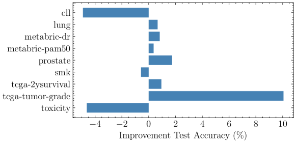
Figure 7: Ablation on including the WPN in WPFS. We trained a WPFS model for each dataset with and without the WPN. We tuned the sparsity hyper-parameter $\lambda\in\{0,3e-5\}$ for each dataset and selected the best-performing model based on the validation cross-entropy. The x-axis represents the absolute improvement in the test accuracy by including the WPN. The WPN improves the overall performance across most datasets, except in the cases of ‘cll’ and ‘toxicity’ when it exhibits subpar but comparable performance.

Appendix E Ablation Sparsity Loss Hyper-parameter $\lambda$ on the Classification Accuracy

Table 9: Test accuracy of WPFS trained with different sparsity loss hyper-parameter $\lambda$. We report the mean balanced accuracy and standard deviation, averaged over 25 runs.

Sparsity parameter	$\lambda=0$	$\lambda=3e-6$	$\lambda=3e-5$	$\lambda=3e-4$	$\lambda=3e-3$	$\lambda=1e-2$
cll	$76,05\pm 7,26$	$78,06\pm 7,98$	$78,27\pm 10,05$	$79,14\pm 4,45$	$77,5\pm 7,35$	$75,49\pm 9,77$
lung	$94,65\pm 4,83$	$94,09\pm 4,81$	$94,83\pm 4,2$	$93,36\pm 5,76$	$93,89\pm 4,99$	$93,56\pm 4,96$
metabric-dr	$59,05\pm 8,62$	$58,9\pm 6,99$	$56,89\pm 8,4$	$57,63\pm 10,61$	$54,6\pm 8,48$	$53,13\pm 7,4$
metabric-pam50	$95,5\pm 4,8$	$95,96\pm 4,11$	$95,86\pm 4,55$	$94,63\pm 4,64$	$92,76\pm 7,78$	$92,45\pm 6,03$
prostate	$89\pm 7,62$	$89.11\pm 6.53$	$87,84\pm 6,26$	$88,42\pm 5,69$	$89,15\pm 6,73$	$86.77\pm 5.39$
smk	$66,08\pm 6,09$	$63,91\pm 7,43$	$66,89\pm 6,21$	$64,16\pm 6,45$	$65,84\pm 6,09$	$62,73\pm 8,63$
tcga-2ysurvival	$56,52\pm 6,24$	$57,04\pm 6,66$	$59,54\pm 6,93$	$57,03\pm 5,89$	$57,44\pm 5,81$	$56,41\pm 7.55$
tcga-tumor-grade	$55,29\pm 11,29$	$51,99\pm 9.04$	$55,91\pm 8,57$	$52,25\pm 10,19$	$51,78\pm 9,86$	$53,23\pm 11.47$
toxicity	$88,01\pm 6,31$	$86,43\pm 5,38$	$88,29\pm 5,27$	$83,83\pm 6,98$	$86,8\pm 7,02$	$82,78\pm 7,11$

Appendix F Ablation Varying Dataset Size

We performed ablations with varying numbers of samples from the ‘metabric-dr’ and ‘metabric-pam50’ datasets. We trained WPFS and MLP using the settings presented in Appx. A.3. For WPFS, we used the best sparsity hyper-parameter for dataset size $200$ ($\lambda=0$ for ‘metabric-dr’ and $\lambda=3e-6$ for ‘metabric-pam50’), and we did not tune it for different sizes of the dataset – though that is likely to improve the performance of WPFS. For each dataset, we perform $5$-fold cross-validation repeated $5$ times, resulting in $25$ runs. We randomly select $10\%$ of the training data for validation for each fold, and we report the mean and standard deviation of the balanced accuracy across all $25$ runs.

Figure 8 compares the test accuracy of WPFS with an MLP. On ‘metabric-dr’, we found that WPFS outperforms an MLP with very few samples, but the performance of the two models converges as the dataset size increases.

For completeness, we include the train/valid/test accuracy of WPFS and MLP on both datasets: ‘metabric-dr’ in Figure 9 and ‘metabric-pam50’ in Figure 10. As the dataset size increases, the generalisation gap between train-valid decreases, as it becomes harder to overfit a large training dataset. The test performance increases with the dataset size, and the instability decreases. Although the test performance of the two models converges for large dataset sizes, the generalisation gap of WPFS is smaller, indicating smaller overfitting.

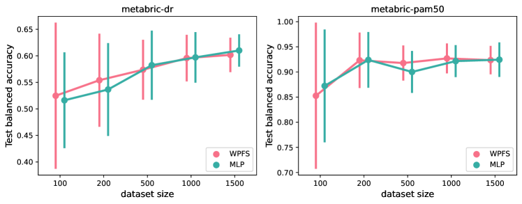
Figure 8: Test performance of WPFS and MLP on two datasets of varying sizes. We report the mean and standard deviation over 25 runs. Left: On ‘metabric-dr’ – a task on which all models obtain small accuracy – we found that WPFS outperforms an MLP with very few samples. As the dataset increases, the instability decreases, and the performance of the two models becomes comparable. Right: The models perform comparably, likely because ‘metabric-pam50’ is an easy task on which all models obtain high accuracy.

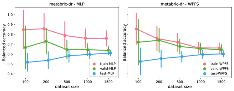
Figure 9: The train/valid/test performance of an MLP (left) and WPFS (right) on ‘metabric-dr’. We report the mean and standard deviation accuracy over 25 runs. As the dataset size increases, the generalisation gap between train-valid decreases, as it becomes harder to overfit a large training dataset. The test performance increases with the dataset size, and the instability decreases. Although the test performance of the two models converges for large dataset sizes, the generalisation gap of WPFS is smaller, indicating smaller overfitting.

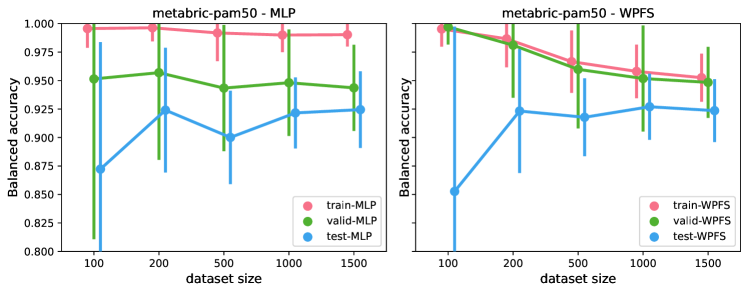
Figure 10: The train/valid/test performance of an MLP (left) and WPFS (right) on ‘metabric-pam50’. We report the mean and standard deviation accuracy over 25 runs. As the dataset size increases, the instability decreases, and the generalisation gap between train-valid decreases as it becomes harder to overfit a large training dataset. The test performance remains constant from around 200 samples, likely because the models already reach high test accuracy. Although the test performance of the two models converges for large dataset sizes, the generalisation gap of WPFS is smaller, indicating smaller overfitting.

Appendix G Complete Results on Classification Accuracy

Table 10: Evaluation on $9$ real-world biomedical datasets. We report the mean balanced accuracy and standard deviation averaged over $25$ runs.

Method	cll	lung	metabric-dr	metabric-pam50	prostate	smk	tcga-2ysurvival	tcga-tumor-grade	toxicity
DietNetworks	$68.84\pm 9.21$	$90.43\pm 6.23$	$56.98\pm 8.70$	$95.02\pm 4.77$	$81.71\pm 11.04$	$62.71\pm 9.38$	$53.62\pm 5.46$	$46.69\pm 7.11$	$82.13\pm 7.42$
FsNet	$66.38\pm 9.22$	$91.75\pm 3.04$	$56.92\pm 10.13$	$83.86\pm 8.16$	$84.74\pm 9.80$	$56.27\pm 9.23$	$53.83\pm 7.94$	$45.94\pm 9.80$	$60.26\pm 8.10$
CAE	$71.94\pm 13.45$	$85\pm 5.04$	$57.35\pm 9.37$	$95.78\pm 3.61$	$87.6\pm 7.84$	$59.96\pm 10.98$	$52.79\pm 8.34$	$40.69\pm 7.36$	$60.36\pm 11.29$
LassoNet	$30.63\pm 8.68$	$25.11\pm 9.81$	$48.88\pm 5.74$	$48.81\pm 10.82$	$54.78\pm 10.58$	$51.04\pm 8.56$	$46.08\pm 9.21$	$33.49\pm 7.55$	$26.67\pm 8.66$
DNP	$85.12\pm 5.46$	$92.83\pm 5.65$	$55.79\pm 7.06$	$93.56\pm 5.54$	$90.25\pm 5.98$	$66.89\pm 7.64$	$58.13\pm 8.2$	$44.71\pm 5.98$	$93.5\pm 6.17$
SPINN	$85.34\pm 5.47$	$92.26\pm 6.68$	$56.13\pm 7.24$	$93.56\pm 5.54$	$89.27\pm 5.91$	$68.43\pm 7.99$	$57.70\pm 7.07$	$44.28\pm 6.84$	$93.5\pm 4.85$
TabNet	$57.81\pm 9.97$	$77.65\pm 12.92$	$49.18\pm 9.60$	$83.60\pm 11.44$	$65.66\pm 14.75$	$54.57\pm 8.72$	$51.58\pm 9.90$	$39.34\pm 7.92$	$40.06\pm 11.37$
MLP	$78.30\pm 8.98$	$94.20\pm 4.94$	$59.56\pm 5.50$	$94.31\pm 5.39$	$88.76\pm 5.55$	$64.42\pm 8.44$	$56.28\pm 6.72$	$48.19\pm 7.75$	$93.21\pm 6.13$
Random Forest	$82.06\pm 6.51$	$91.81\pm 6.94$	$51.38\pm 3.78$	$89.11\pm 6.59$	$90.78\pm 7.17$	$68.16\pm 7.56$	$61.30\pm 6.00$	$50.93\pm 8.48$	$80.75\pm 6.75$
LightGBM	$85.59\pm 6.51$	$93.42\pm 5.91$	$58.23\pm 8.55$	$94.97\pm 5.19$	$91.38\pm 5.71$	$65.70\pm 7.46$	$57.08\pm 7.86$	$49.11\pm 10.32$	$82.40\pm 6.48$
WPFS (ours)	$79.14\pm 4.45$ $[\lambda=3e-4]$	$94.83\pm 4.2$ $[\lambda=3e-5]$	$59.05\pm 8.62$ $[\lambda=0]$	$95.96\pm 4.11$ $[\lambda=3e-6]$	$89.15\pm 6.73$ $[\lambda=3e-3]$	$66.89\pm 6.21$ $[\lambda=3e-5]$	$59.54\pm 6.93$ $[\lambda=3e-5]$	$55.91\pm 8.57$ $[\lambda=3e-5]$	$88.29\pm 5.27$ $[\lambda=3e-5]$

Appendix H Ablation Sparsity Loss Hyper-parameter $\lambda$ on the Feature Importance Scores

We investigate the effect of the sparsity loss hyper-parameter $\lambda$ on the distribution of feature importance scores. For each dataset, we show three runs trained on different data splits. Across datasets, increasing $\lambda$ leads to fewer selected features. Notice that WPFS is uncertain which features are important in tasks with low test performance (e.g., Figure 13), it provides almost binary feature importance on tasks with high test performance (e.g., Figure 14).

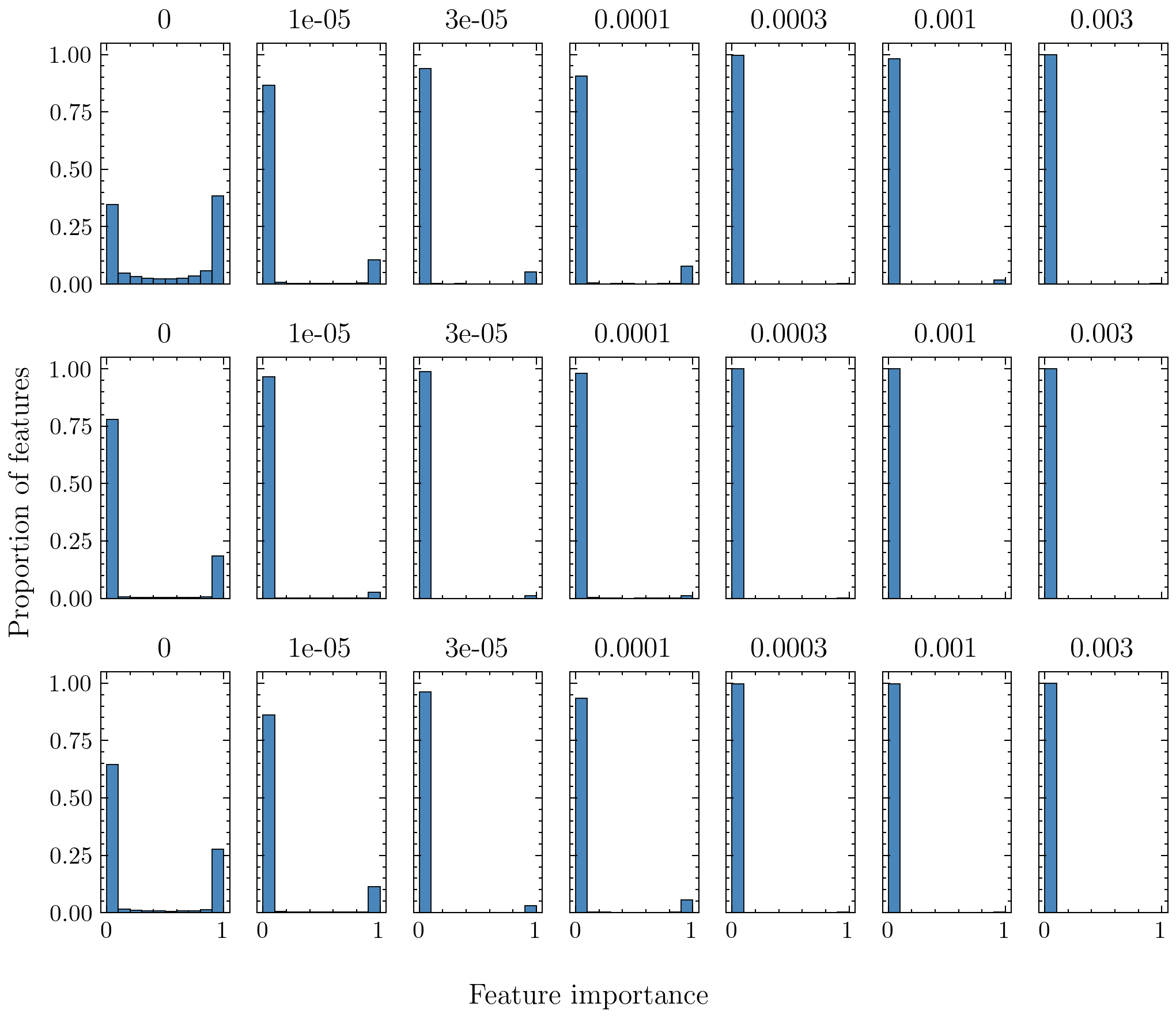
Figure 11: Feature importance for dataset cll, when increasing the sparsity hyper-parameters $\lambda$. Each row represents one randomly chosen training split, and each column represent a different sparsity hyper-parameter. Notice that increasing $\lambda$ leads to a larger proportion of features considered irrelevant (i.e., their feature importance scores tend to zero).

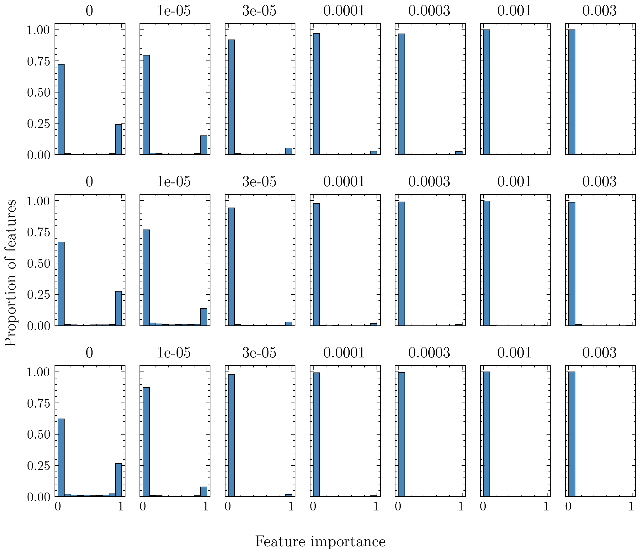
Figure 12: Feature importance scores for dataset lung, when increasing the sparsity hyper-parameters $\lambda$. Each row represents one randomly chosen training split, and each column represent a different sparsity hyper-parameter. Notice that increasing $\lambda$ leads to a larger proportion of features considered irrelevant (i.e., their feature importance scores tend to zero).

Figure 13: Feature importance scores for dataset metabric-dr, when increasing the sparsity hyper-parameters $\lambda$. Each row represents one randomly chosen training split, and each column represent a different sparsity hyper-parameter. Notice that increasing $\lambda$ leads to a larger proportion of features considered irrelevant (i.e., their feature importance scores tend to zero).

Figure 14: Feature importance for dataset metabric-pam50, when increasing the sparsity hyper-parameters $\lambda$. Each row represents one randomly chosen training split, and each column represent a different sparsity hyper-parameter. Notice that increasing $\lambda$ leads to a larger proportion of features considered irrelevant (i.e., their feature importance scores tend to zero).

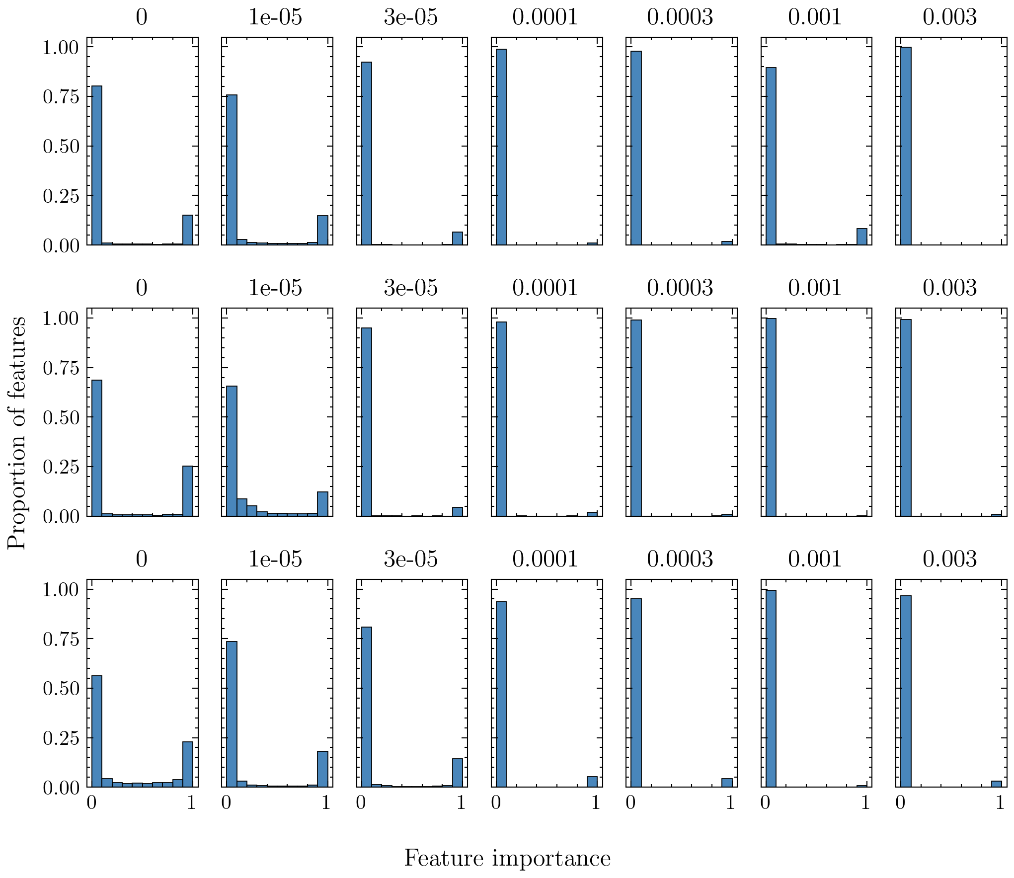
Figure 15: Feature importance scores for dataset prostate, when increasing the sparsity hyper-parameters $\lambda$. Each row represents one randomly chosen training split, and each column represent a different sparsity hyper-parameter. Notice that increasing $\lambda$ leads to a larger proportion of features considered irrelevant (i.e., their feature importance scores tend to zero).

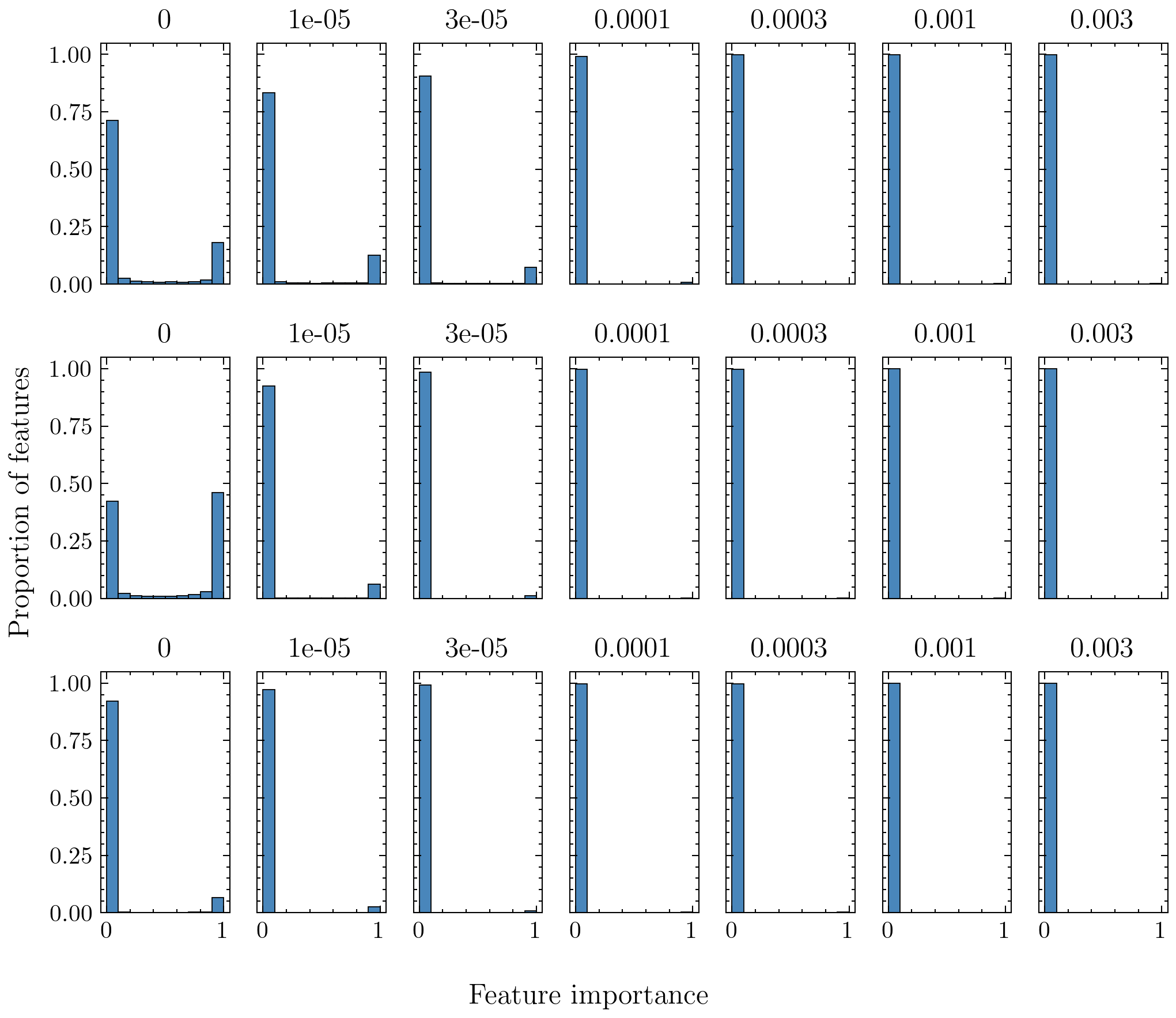
Figure 16: Feature importance scores for dataset smk, when increasing the sparsity hyper-parameters $\lambda$. Each row represents one randomly chosen training split, and each column represent a different sparsity hyper-parameter. Notice that increasing $\lambda$ leads to a larger proportion of features considered irrelevant (i.e., their feature importance scores tend to zero).

Figure 17: Feature importance scores for dataset tcga-2ysurvival, when increasing the sparsity hyper-parameters $\lambda$. Each row represents one randomly chosen training split, and each column represent a different sparsity hyper-parameter. Notice that increasing $\lambda$ leads to a larger proportion of features considered irrelevant (i.e., their feature importance scores tend to zero).

Figure 18: Feature importance scores for dataset tcga-tumor-grade, when increasing the sparsity hyper-parameters $\lambda$. Each row represents one randomly chosen training split, and each column represent a different sparsity hyper-parameter. Notice that increasing $\lambda$ leads to a larger proportion of features considered irrelevant (i.e., their feature importance scores tend to zero).

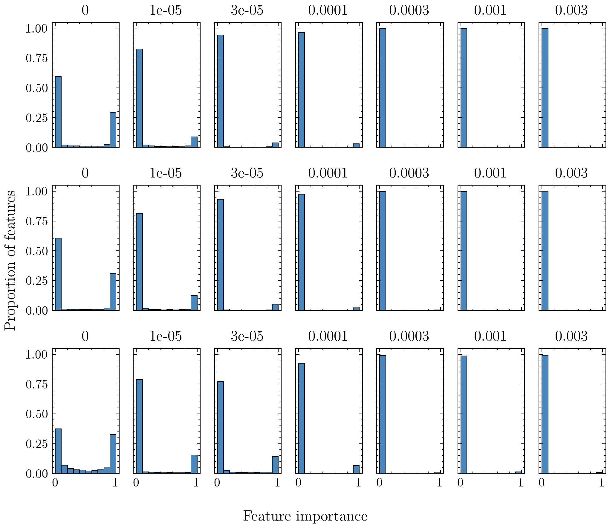
Figure 19: Feature importance scores for dataset toxicity, when increasing the sparsity hyper-parameters $\lambda$. Each row represents one randomly chosen training split, and each column represent a different sparsity hyper-parameter. Notice that increasing $\lambda$ leads to a larger proportion of features considered irrelevant (i.e., their feature importance scores tend to zero).

Appendix I Training Dynamics for WPFS and MLP

I.1 Loss curves

We show the loss curves trends of six randomly selected runs for each dataset. We selected the model with the smallest validation loss for each run, and we display its performance (test balanced accuracy in the title and the train/validation balanced accuracy in the legend). As a general trend, we observe that the loss curve is a good indicator of the validation performance. When one loss diverges, the corresponding model has lower validation accuracy (see Figure 26). However, there is not a strong correlation between validation and test performance. We believe this is expected because the datasets have few samples, and we use $10\%$ of data for validation and $20\%$ for testing.

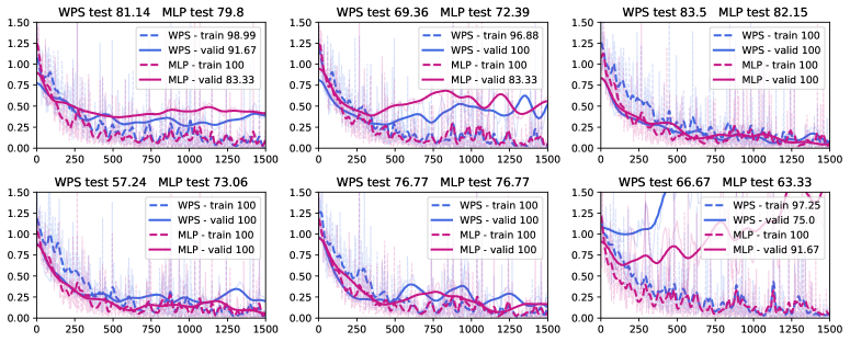
Figure 20: Loss curve trends for dataset ‘cll’ for 9 randomly selected runs. The x-axis represents the iteration, and the y-axis represents the weighted cross-entropy. Each subfigure displayes the test accuracy in the title, and the train/validation accuracy in the legend.

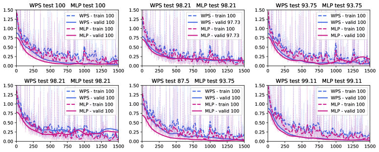
Figure 21: Loss curve trends for dataset ‘lung’ for 9 randomly selected runs. The x-axis represents the iteration, and the y-axis represents the weighted cross-entropy. Each subfigure displayes the test accuracy in the title, and the train/validation accuracy in the legend.

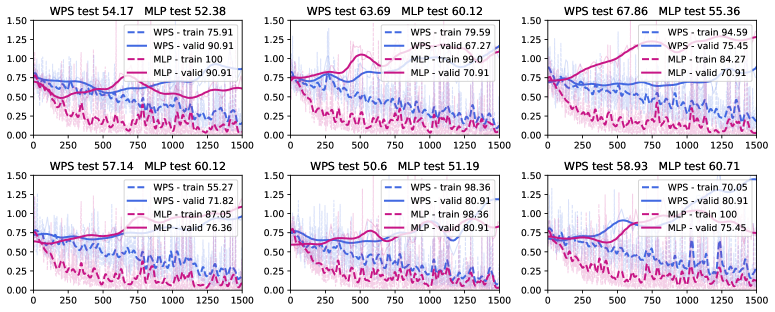
Figure 22: Loss curve trends for dataset ‘metabric-dr’ for 9 randomly selected runs. The x-axis represents the iteration, and the y-axis represents the weighted cross-entropy. Each subfigure displayes the test accuracy in the title, and the train/validation accuracy in the legend.

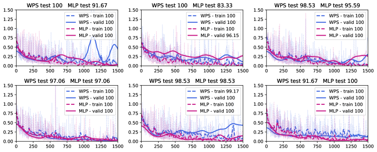
Figure 23: Loss curve trends for dataset ‘metabric-pam50’ for 9 randomly selected runs. The x-axis represents the iteration, and the y-axis represents the weighted cross-entropy. Each subfigure displayes the test accuracy in the title, and the train/validation accuracy in the legend.

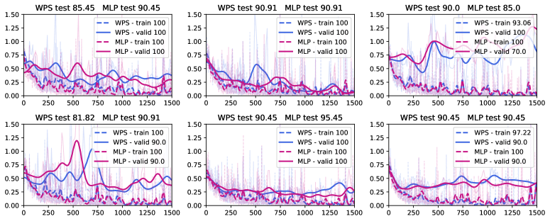
Figure 24: Loss curve trends for dataset ‘prostate’ for 9 randomly selected runs. The x-axis represents the iteration, and the y-axis represents the weighted cross-entropy. Each subfigure displayes the test accuracy in the title, and the train/validation accuracy in the legend.

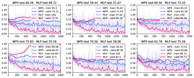
Figure 25: Loss curve trends for dataset ‘smk’ for 9 randomly selected runs. The x-axis represents the iteration, and the y-axis represents the weighted cross-entropy. Each subfigure displayes the test accuracy in the title, and the train/validation accuracy in the legend.

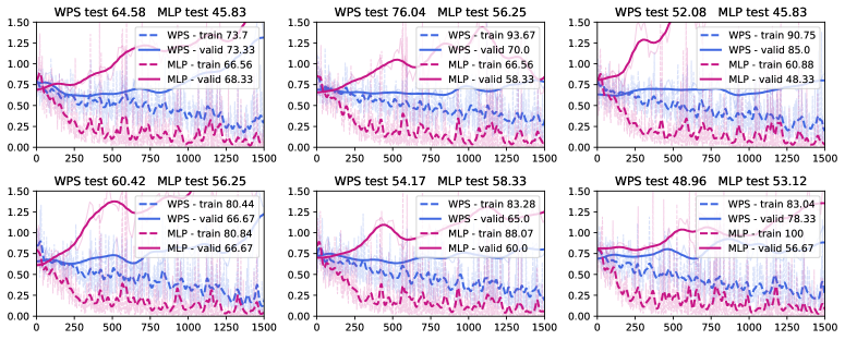
Figure 26: Loss curve trends for dataset ‘tcga-2ysurvival’ for 9 randomly selected runs. The x-axis represents the iteration, and the y-axis represents the weighted cross-entropy. Each subfigure displayes the test accuracy in the title, and the train/validation accuracy in the legend.

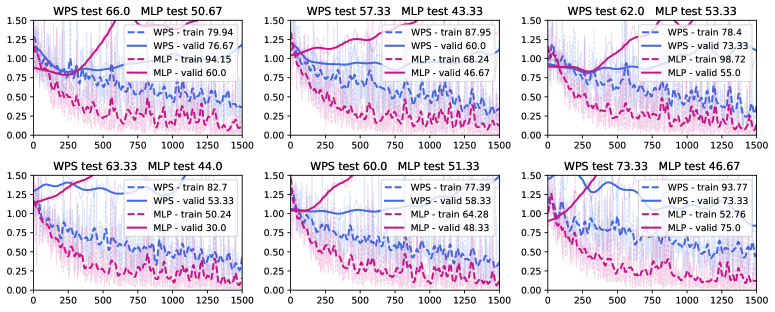
Figure 27: Loss curve trends for dataset ‘tcga-tumor-grade’ for 9 randomly selected runs. The x-axis represents the iteration, and the y-axis represents the weighted cross-entropy. Each subfigure displayes the test accuracy in the title, and the train/validation accuracy in the legend.

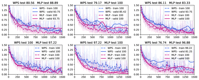
Figure 28: Loss curve trends for dataset ‘toxicity’ for 9 randomly selected runs. The x-axis represents the iteration, and the y-axis represents the weighted cross-entropy. Each subfigure displayes the test accuracy in the title, and the train/validation accuracy in the legend.

References

- Alexandrov et al. (2013) Alexandrov, L. B.; Nik-Zainal, S.; Wedge, D. C.; Campbell, P. J.; and Stratton, M. R. 2013. Deciphering signatures of mutational processes operative in human cancer. Cell reports, 3(1): 246–259.
- Alter, Brown, and Botstein (2000) Alter, O.; Brown, P. O.; and Botstein, D. 2000. Singular value decomposition for genome-wide expression data processing and modeling. Proceedings of the National Academy of Sciences, 97(18): 10101–10106.
- Arık and Pfister (2021) Arık, S. O.; and Pfister, T. 2021. Tabnet: Attentive interpretable tabular learning. In AAAI Conference on Artificial Intelligence, volume 35, 6679–6687.
- Bach (2017) Bach, F. 2017. Breaking the curse of dimensionality with convex neural networks. The Journal of Machine Learning Research, 18(1): 629–681.
- Bajwa et al. (2016) Bajwa, G.; DeBerardinis, R. J.; Shao, B.; Hall, B.; Farrar, J. D.; and Gill, M. A. 2016. Cutting edge: Critical role of glycolysis in human plasmacytoid dendritic cell antiviral responses. The Journal of Immunology, 196(5): 2004–2009.
- Balin, Abid, and Zou (2019) Balin, M. F.; Abid, A.; and Zou, J. Y. 2019. Concrete Autoencoders: Differentiable Feature Selection and Reconstruction. In International Conference on Machine Learning, 444–453.
- Bhattacharjee et al. (2001) Bhattacharjee, A.; Richards, W. G.; Staunton, J.; Li, C.; Monti, S.; Vasa, P.; Ladd, C.; Beheshti, J.; Bueno, R.; Gillette, M.; et al. 2001. Classification of human lung carcinomas by mRNA expression profiling reveals distinct adenocarcinoma subclasses. Proceedings of the National Academy of Sciences, 98(24): 13790–13795.
- Breiman (2001) Breiman, L. 2001. Random forests. Machine learning, 45(1): 5–32.
- Curtis et al. (2012) Curtis, C.; Shah, S. P.; Chin, S.-F.; Turashvili, G.; Rueda, O. M.; Dunning, M. J.; Speed, D.; Lynch, A. G.; Samarajiwa, S.; Yuan, Y.; et al. 2012. The genomic and transcriptomic architecture of 2,000 breast tumours reveals novel subgroups. Nature, 486(7403): 346–352.
- Feng and Simon (2017) Feng, J.; and Simon, N. 2017. Sparse-input neural networks for high-dimensional nonparametric regression and classification. arXiv preprint arXiv:1711.07592.
- Glorot and Bengio (2010) Glorot, X.; and Bengio, Y. 2010. Understanding the difficulty of training deep feedforward neural networks. In Proceedings of the thirteenth international conference on artificial intelligence and statistics, 249–256. JMLR Workshop and Conference Proceedings.
- Gorishniy et al. (2021) Gorishniy, Y. V.; Rubachev, I.; Khrulkov, V.; and Babenko, A. 2021. Revisiting Deep Learning Models for Tabular Data. In Advances in Neural Information Processing Systems.
- Ha, Dai, and Le (2017) Ha, D.; Dai, A. M.; and Le, Q. V. 2017. HyperNetworks. International Conference on Learning Representations.
- Haslinger et al. (2004) Haslinger, C.; Schweifer, N.; Stilgenbauer, S.; Dohner, H.; Lichter, P.; Kraut, N.; Stratowa, C.; and Abseher, R. 2004. Microarray gene expression profiling of B-cell chronic lymphocytic leukemia subgroups defined by genomic aberrations and VH mutation status. Journal of Clinical Oncology, 22(19): 3937–3949.
- Hazimeh et al. (2020) Hazimeh, H.; Ponomareva, N.; Mol, P.; Tan, Z.; and Mazumder, R. 2020. The tree ensemble layer: Differentiability meets conditional computation. In International Conference on Machine Learning, 4138–4148. PMLR.
- He et al. (2015) He, K.; Zhang, X.; Ren, S.; and Sun, J. 2015. Delving deep into rectifiers: Surpassing human-level performance on imagenet classification. In Proceedings of the IEEE international conference on computer vision, 1026–1034.
- Huang et al. (2020) Huang, X.; Khetan, A.; Cvitkovic, M. W.; and Karnin, Z. S. 2020. TabTransformer: Tabular Data Modeling Using Contextual Embeddings. arXiv, abs/2012.06678.
- Ioffe and Szegedy (2015) Ioffe, S.; and Szegedy, C. 2015. Batch normalization: Accelerating deep network training by reducing internal covariate shift. In International Conference on Machine Learning, 448–456. PMLR.
- Kadra et al. (2021) Kadra, A.; Lindauer, M.; Hutter, F.; and Grabocka, J. 2021. Well-tuned Simple Nets Excel on Tabular Datasets. Advances in Neural Information Processing Systems, 34.
- Katzir, Elidan, and El-Yaniv (2020) Katzir, L.; Elidan, G.; and El-Yaniv, R. 2020. Net-DNF: Effective deep modeling of tabular data. In International Conference on Learning Representations.
- Ke et al. (2017) Ke, G.; Meng, Q.; Finley, T.; Wang, T.; Chen, W.; Ma, W.; Ye, Q.; and Liu, T.-Y. 2017. Lightgbm: A highly efficient gradient boosting decision tree. Advances in Neural Information Processing Systems, 30.
- Kim and Park (2007) Kim, H.; and Park, H. 2007. Sparse non-negative matrix factorizations via alternating non-negativity-constrained least squares for microarray data analysis. Bioinformatics, 23(12): 1495–1502.
- Lemhadri, Ruan, and Tibshirani (2021) Lemhadri, I.; Ruan, F.; and Tibshirani, R. 2021. Lassonet: Neural networks with feature sparsity. In International Conference on Artificial Intelligence and Statistics, 10–18. PMLR.
- Li et al. (2018) Li, J.; Cheng, K.; Wang, S.; Morstatter, F.; Trevino, R. P.; Tang, J.; and Liu, H. 2018. Feature selection: A data perspective. ACM Computing Surveys (CSUR), 50(6): 94.
- Liberzon et al. (2015) Liberzon, A.; Birger, C.; Thorvaldsdóttir, H.; Ghandi, M.; Mesirov, J. P.; and Tamayo, P. 2015. The molecular signatures database hallmark gene set collection. Cell systems, 1(6): 417–425.
- Liu et al. (2017) Liu, B.; Wei, Y.; Zhang, Y.; and Yang, Q. 2017. Deep Neural Networks for High Dimension, Low Sample Size Data. In International Joint Conference on Artificial Intelligence, 2287–2293.
- Loshchilov and Hutter (2017) Loshchilov, I.; and Hutter, F. 2017. SGDR: Stochastic Gradient Descent with Warm Restarts. arXiv: Learning.
- Loshchilov and Hutter (2019) Loshchilov, I.; and Hutter, F. 2019. Decoupled Weight Decay Regularization. In International Conference on Learning Representations.
- Paszke et al. (2019) Paszke, A.; Gross, S.; Massa, F.; Lerer, A.; Bradbury, J.; Chanan, G.; Killeen, T.; Lin, Z.; Gimelshein, N.; Antiga, L.; et al. 2019. Pytorch: An imperative style, high-performance deep learning library. Advances in Neural Information Processing Systems, 32.
- Pedregosa et al. (2011) Pedregosa, F.; Varoquaux, G.; Gramfort, A.; Michel, V.; Thirion, B.; Grisel, O.; Blondel, M.; Prettenhofer, P.; Weiss, R.; Dubourg, V.; et al. 2011. Scikit-learn: Machine learning in Python. the Journal of machine Learning research, 12: 2825–2830.
- Popov, Morozov, and Babenko (2020) Popov, S.; Morozov, S.; and Babenko, A. 2020. Neural Oblivious Decision Ensembles for Deep Learning on Tabular Data. In International Conference on Learning Representations.
- Qin et al. (2021) Qin, Z.; Yan, L.; Zhuang, H.; Tay, Y.; Pasumarthi, R. K.; Wang, X.; Bendersky, M.; and Najork, M.-A. 2021. Are Neural Rankers still Outperformed by Gradient Boosted Decision Trees? In International Conference on Learning Representations.
- Romero et al. (2017) Romero, A.; Carrier, P. L.; Erraqabi, A.; Sylvain, T.; Auvolat, A.; Dejoie, E.; Legault, M.-A.; Dubé, M.-P.; Hussin, J. G.; and Bengio, Y. 2017. Diet Networks: Thin Parameters for Fat Genomics. In International Conference on Learning Representations.
- Simon et al. (2013) Simon, N.; Friedman, J.; Hastie, T.; and Tibshirani, R. 2013. A sparse-group lasso. Journal of computational and graphical statistics, 22(2): 231–245.
- Singh et al. (2020) Singh, D.; Climente-González, H.; Petrovich, M.; Kawakami, E.; and Yamada, M. 2020. Fsnet: Feature selection network on high-dimensional biological data. arXiv preprint arXiv:2001.08322.
- Singh et al. (2002) Singh, D.; Febbo, P. G.; Ross, K.; Jackson, D. G.; Manola, J.; Ladd, C.; Tamayo, P.; Renshaw, A. A.; D’Amico, A. V.; Richie, J. P.; et al. 2002. Gene expression correlates of clinical prostate cancer behavior. Cancer cell, 1(2): 203–209.
- Spira et al. (2007) Spira, A.; Beane, J. E.; Shah, V.; Steiling, K.; Liu, G.; Schembri, F.; Gilman, S.; Dumas, Y.-M.; Calner, P.; Sebastiani, P.; et al. 2007. Airway epithelial gene expression in the diagnostic evaluation of smokers with suspect lung cancer. Nature medicine, 13(3): 361–366.
- Srivastava et al. (2014) Srivastava, N.; Hinton, G.; Krizhevsky, A.; Sutskever, I.; and Salakhutdinov, R. 2014. Dropout: a simple way to prevent neural networks from overfitting. The journal of machine learning research, 15(1): 1929–1958.
- Taslaman and Nilsson (2012) Taslaman, L.; and Nilsson, B. 2012. A framework for regularized non-negative matrix factorization, with application to the analysis of gene expression data. PloS one, 7(11): e46331.
- Tibshirani (1996) Tibshirani, R. 1996. Regression shrinkage and selection via the lasso. Journal of the Royal Statistical Society: Series B (Methodological), 58(1): 267–288.
- Tomczak, Czerwińska, and Wiznerowicz (2015) Tomczak, K.; Czerwińska, P.; and Wiznerowicz, M. 2015. The Cancer Genome Atlas (TCGA): an immeasurable source of knowledge. Contemporary oncology, 19(1A): A68.
- Yang, Lindenbaum, and Kluger (2022) Yang, J.; Lindenbaum, O.; and Kluger, Y. 2022. Locally Sparse Neural Networks for Tabular Biomedical Data. In International Conference in Machine Learning.
- Yang, Morillo, and Hospedales (2018) Yang, Y.; Morillo, I. G.; and Hospedales, T. M. 2018. Deep Neural Decision Trees. International Conference in Machine Learning - Workshop on Human Interpretability in Machine Learning (WHI).
- Yoon, Jordon, and van der Schaar (2018) Yoon, J.; Jordon, J.; and van der Schaar, M. 2018. INVASE: Instance-wise variable selection using neural networks. In International Conference on Learning Representations.