Learning from Good Trajectories in Offline Multi-Agent Reinforcement Learning

Abstract

Offline multi-agent reinforcement learning (MARL) aims to learn effective multi-agent policies from pre-collected datasets, which is an important step toward the deployment of multi-agent systems in real-world applications. However, in practice, each individual behavior policy that generates multi-agent joint trajectories usually has a different level of how well it performs. e.g., an agent is a random policy while other agents are medium policies. In the cooperative game with global reward, one agent learned by existing offline MARL often inherits this random policy, jeopardizing the performance of the entire team. In this paper, we investigate offline MARL with explicit consideration on the diversity of agent-wise trajectories and propose a novel framework called Shared Individual Trajectories (SIT) to address this problem. Specifically, an attention-based reward decomposition network assigns the credit to each agent through a differentiable key-value memory mechanism in an offline manner. These decomposed credits are then used to reconstruct the joint offline datasets into prioritized experience replay with individual trajectories, thereafter agents can share their good trajectories and conservatively train their policies with a graph attention network (GAT) based critic. We evaluate our method in both discrete control (i.e., StarCraft II and multi-agent particle environment) and continuous control (i.e., multi-agent mujoco). The results indicate that our method achieves significantly better results in complex and mixed offline multi-agent datasets, especially when the difference of data quality between individual trajectories is large.

Introduction

Multi-agent reinforcement learning (MARL) has shown its powerful ability to solve many complex decision-making tasks. e.g., game playing (Samvelyan et al. 2019). However, deploying MARL to practical applications is not easy since interaction with the real world is usually prohibitive, costly, or risky (Garcıa 2015), e.g., autonomous driving (Shalev-Shwartz, Shammah, and Shashua 2016). Thus offline MARL, which aims to learn multi-agent policies in the previously-collected, non-expert datasets without further interaction with environments, is an ideal way to cope with practical problems.

Recently, Yang et al. (2021) first investigated offline MARL and found that multi-agent systems are more susceptible to extrapolation error (Fujimoto, Meger, and Precup 2019), i.e., a phenomenon in which unseen state-action pairs are erroneously estimated, compared to offline single-agent reinforcement learning (RL) (Fujimoto, Meger, and Precup 2019; Kumar et al. 2019; Wu, Tucker, and Nachum 2019; Kumar et al. 2020; Fujimoto and Gu 2021). Then they proposed implicit constraint Q-learning (ICQ), which can effectively alleviate this problem by only trusting the state-action pairs given in the dataset for value estimation.

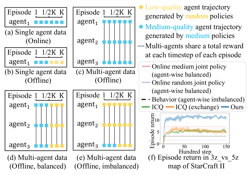
Figure 1: (a)$\sim$(e) Data composition of data replay in episodic online/offline RL/MARL, where the online learning agents in (a) and (c) are assumed to be medium policies. (f) Episode return in 3z_vs_5z map of StarCraft II with the offline data structure of (e).

In this paper, we point out that in addition to extrapolation error, the diversity of trajectories in the offline multi-agent dataset also deserves attention since the composition of this dataset is much more complex than its single-agent version. For better illustration, we briefly summarize the data quality of data replay in episodic online/offline RL/MARL as is shown in Figure 1. In online settings, since the data replay is updated rollingly based on the learning policy, the quality of all data points is approximately the same as is shown in Figure 1(a) and Figure 1(c), where line connections in Figure 1(c) represent multi-agent systems only provide one global reward at each timestep of each episode. In offline settings, there is no restriction on the quality of collected data, thus the single-agent data replay usually contains multi-source and suboptimal data as is shown in Figure 1(b). Figure 1(d) directly extends the offline single-agent data composition to a multi-agent version. However, in practical tasks, each individual trajectory in an offline multi-agent joint trajectory usually has a different data quality, as is shown in Figure 1(e). For example, consider the task that two robotic arms (agents) work together to lift a large circular object, and the reward is the height of the center of mass. Suppose that two workers operate two robotic arms simultaneously to collect offline data, but they have different levels of proficiency in robotic arm operation. The offline joint data generated in this case is an agent-wise imbalanced multi-agent dataset.

To investigate the performance of the current state-of-the-art offline MARL algorithm, ICQ, on the imbalanced dataset, we test it on the 3s_vs_5z map in StarCraft II (Samvelyan et al. 2019). Specifically, as is shown in Figure 1(f), we first obtain random joint policy (violet dotted) and medium joint policy (red dotted) through online training, and then utilize these two joint policies to construct an agent-wise imbalanced dataset with the data structure of Figure 1(e). We can observe that the performance of ICQ (green) is lower than that of the online medium joint policy (red dotted), as ${\rm agent_{1}}$ and ${\rm agent_{2}}$ may inherit the random behavior policies that generate the data. One might attempt to solve this issue of ICQ by randomly exchanging local observations and actions among agents, so that ${\rm agent_{1}}$ and ${\rm agent_{2}}$ can share some medium-quality individual trajectories of ${\rm agent_{3}}$. Unfortunately, the performance of this alternative (orange) is similar to ICQ, since the proportion of the medium-quality individual data in the data replay does not change under the constraint of the total reward.

In this paper, we propose a novel algorithmic framework called Shared Individual Trajectories (SIT) to address this problem. It first learns an Attention-based Reward Decomposition Network with Ensemble Mechanism (ARDNEM), which assigns credits to each agent through a differentiable key-value memory mechanism in an offline manner. Then these credits are used to reconstruct the original joint trajectories into Decomposed Prioritized Experience Replay (DPER) with individual trajectories, thereafter agents can share their good trajectories and conservatively train their policies with a graph attention network based critic. Extensive experiments on both discrete control (i.e., StarCraft II and multi-agent particle environment) and continuous control (i.e., multi-agent mujoco) indicate that our method achieves significantly better results in complex and mixed offline multi-agent datasets, especially when the difference of data quality between individual trajectories is large.

Related Work

Offline MARL.

Recently, Yang et al. (2021) first explored offline MARL and found that multi-agent systems are more susceptible to extrapolation error (Fujimoto, Meger, and Precup 2019) compared to offline single-agent RL (Fujimoto, Meger, and Precup 2019; Kumar et al. 2020; Fujimoto and Gu 2021), and then they proposed implicit constraint Q-learning (ICQ) to solve this problem. Jiang and Lu (2021a) investigated the mismatch problem of transition probabilities in fully decentralized offline MARL. However, they assume that each agent makes the decision based on the global state and the reward output by the environment can accurately evaluate each agent’s action. This is fundamentally different from our work since we focus on the partially observable setting in global reward games (Chang, Ho, and Kaelbling 2003), which is a more practical situation. Other works (Meng et al. 2021; Jiang and Lu 2021b) have made some progress in offline MARL training with online fine-tuning. Unfortunately, all the existing methods neglect to investigate the diversity of trajectories in offline multi-agent datasets, while we take the first step to fill this gap.

Multi-agent credit assignment.

In cooperative multi-agent environments, all agents receive one total reward. The multi-agent credit assignment aims to correctly allocate the reward signal to each individual agent for a better groups’ coordination (Chang, Ho, and Kaelbling 2003). One popular class of solutions is value decomposition, which can decompose team value function into agent-wise value functions in an online fashion under the framework of the Bellman equation (Sunehag et al. 2018; Rashid et al. 2018; Yang et al. 2020b; Li et al. 2021). Different from these works, in this paper, we focus on explicitly decomposing the total reward into individual rewards in an offline fashion under the regression framework, and these decomposed rewards will be used to reconstruct the offline prioritized dataset.

Experience replay in RL/MARL.

Experience replay, a mechanism for reusing historical data (Lin 1992), is widely used in online RL (Wang et al. 2020a). Many prior works related to it focus on improving data utilization (Schaul et al. 2016; Zha et al. 2019; Oh et al. 2020). e.g., prioritized experience replay (PER) (Schaul et al. 2016) takes temporal-difference (TD) error as a metric for evaluating the value of data and performs importance sampling according to it. Unfortunately, this metric fails in offline training due to severe overestimation in offline scenarios. In online MARL, most works related to the experience replay focus on stable decentralized multi-agent training (Foerster et al. 2017; Omidshafiei et al. 2017; Palmer et al. 2018), but these methods usually rely on some auxiliary information, e.g., training iteration number, timestamp and exploration rate, which often are not provided by the offline settings. SEAC (Christianos, Schäfer, and Albrecht 2020) proposed by Christianos et al. is most related to our work as it also shares individual trajectories among agents during online training. However, SEAC assumes that each agent can directly obtain a local reward and does not consider the importance of each individual trajectory. Instead, we need to decompose the global reward into local rewards in an offline manner, and then determine the quality of the individual trajectory based on the decomposed rewards for priority sampling.

Preliminaries

Figure 2: Overall framework of Shared Individual Trajectories (SIT) in offline MARL

A fully cooperative multi-agent task in the global reward game (Chang, Ho, and Kaelbling 2003) can be described as a Decentralized Partially Observable Markov Decision Process (Dec-POMDP) (Oliehoek and Amato 2016) consisting of a tuple $\langle\emph{N},\mathcal{S},\mathcal{A},\mathcal{T},\mathcal{R},\mathcal{O},\Omega,\gamma\rangle$. Let N represent the number of agents and $\mathcal{S}$ represent the true state space of the environment. At each timestep $t\in\mathcal{Z}^{+}$ of episode $k\in\mathcal{Z}^{+}$, each agent $i\in\emph{N}\equiv\left\{1,\dots,n\right\}$ takes an action $a_{i}\in\mathcal{A}$, forming a joint action $\boldsymbol{a}\in\bm{\mathcal{A}}\equiv\mathcal{A}^{n}$. Let $\mathcal{T}(s^{\prime}|s,\boldsymbol{a}):\mathcal{S}\times\bm{\mathcal{A}}\rightarrow\mathcal{S}$ represent the state transition function. All agents share the global reward function $r(s,\boldsymbol{a}):\mathcal{S}\times\bm{\mathcal{A}}\rightarrow\mathcal{R}$ and $\gamma\in[0,1)$ represents the discount factor. Let $J$ represent the type of agent $i$, which is the prior knowledge given by the environment (Wang et al. 2020b; Yang et al. 2020a). All agent IDs belonging to type $J$ are denoted as $j\in\mathbb{J}$, where $\mathbb{J}$ represents the set of IDs of all agents isomorphic to agent $i$ (including $i$). We consider a partially observable setting in which each agent receives an individual observation $o_{i}\in\Omega$ according to the observation function $\mathcal{O}(s,a):\mathcal{S}\times\mathcal{A}\rightarrow\Omega$. Each agent has an action-observation history $\tau_{i}\in\bm{T}\equiv\left(\Omega\times\mathcal{A}\right)^{t}$, on which it conditions a stochastic policy $\pi_{i}\left(a_{i}|\tau_{i}\right)$. Following Gronauer (2022), we focus on episodic training in this paper.

Methodology

In this section, we propose a new algorithmic framework called Shared Individual Trajectories (SIT) in offline MARL, which can maximally exploit the useful knowledge in the complex and mixed offline multi-agent datasets to boost the performance of multi-agent systems. SIT consists of three stages as shown in Figure 2: Stage I: learning an Attention-based Reward Decomposition Network with Ensemble Mechanism (ARDNEM). Stage II: reconstructing the original joint offline dataset into Decomposed Prioritized Experience Replay (DPER) based on the learned ARDNEM. Stage III: conservative offline actor training with a graph attention network (GAT) based critic on DPER.

Attention-Based Reward Decomposition Network with Ensemble Mechanism

It is a non-trivial problem to evaluate the behavior of individual trajectories in an offline dataset under the global reward games since only one total reward can be accessed in this case. We propose a reward decomposition network, as is shown in Figure 2(a), to solve this problem. Specifically, the individual reward $r_{i}^{t,k}$ at timestep $t$ of episode $k$ can be approximately estimated from the local observation $o_{i}^{t,k}$ and action $a_{i}^{t,k}$ through the reward network $f_{i}$. i.e., $r_{i}^{t,k}=f_{i}(o_{i}^{t,k},a_{i}^{t,k})$. In order to learn the contribution weight $\lambda_{i}^{t,k}$ of each individual reward $r_{i}^{t,k}$ to the total reward, we use the attention mechanism (i.e., the differentiable key-value memory model (Oh et al. 2016)) to achieve this goal. That is, we first encode the global state $s^{t,k}$ and local observation-action pair $(o^{t,k}_{i},a^{t,k}_{i})$ into embedding vectors $e^{t,k}_{s}$ and $e^{t,k}_{i}$ with two multi-layer perceptrons (MLPs) respectively, then we pass the similarity value between the global state’s embedding vector $e^{t,k}_{s}$ and the individual features’ embedding vector $e^{t,k}_{i}$ into a softmax

$$\lambda_{i}^{t,k}\propto\exp((e_{s}^{t,k})^{T}W_{q}^{T}W_{k}e_{i}^{t,k})\,,$$ (1)

where the learnable weight $W_{q}$ and $W_{k}$ transform $e_{s}^{t,k}$ and $e_{i}^{t,k}$ into the query and key. Thus the estimated total reward $\hat{r}_{tot}^{t,k}$ at each timestep $t$ of episode $k$ can be expressed as

$$\hat{r}_{tot}^{t,k}=\sum_{i=1}^{N}\lambda_{i}^{t,k}r_{i}^{t,k}=\sum_{i=1}^{N}\lambda_{i}^{t,k}\cdot f_{i}(o_{i}^{t,k},a_{i}^{t,k})\,.$$ (2)

Since misestimated individual rewards will have a large impact on agent learning, we want to obtain the uncertainty corresponding to each estimated value for correcting subsequent training. Following Chua et al. (2018), we introduce ensemble mechanism (Osband et al. 2016) to meet this goal. i.e., $M$ decomposition networks are learned simultaneously. Finally, our Attention-based Reward Decomposition Network with Ensemble Mechanism (ARDNEM) w.r.t. parameters $\psi$ can be trained on the original joint offline dataset with the following mean-squared error (MSE) loss

$$\mathcal{L}_{{\rm MSE}}(\psi)=\frac{1}{M}\sum_{m=1}^{M}\left(\sum_{i=1}^{N}\lambda_{i,m}^{t,k}\cdot f_{i,m}(o_{i}^{t,k},a_{i}^{t,k})-r_{tot}^{t,k}\right)^{2}\,,$$ (3)

where $r_{tot}^{t,k}$ represents the true total reward in the offline dataset. In practice, the reward network parameters of different agents are shared for the scalability of our method.

Decomposed Prioritized Experience Replay

As is shown in Figure 2(b), after ARDNEM is learned, we can use it to estimate individual rewards for all local trajectories. Specifically, since ARDNEM adopts the ensemble mechanism, we take the mean of $M$ model output $\lambda_{i,m}^{t,k}r_{i,m}^{t,k}$ as the estimation of the weighted individual reward $\hat{r}_{i}^{t,k}$:

$$\hat{r}_{i}^{t,k}=\frac{1}{M}\sum_{m=1}^{M}\lambda_{i,m}^{t,k}r_{i,m}^{t,k}\,.$$ (4)

Its corresponding variance is defined as the uncertainty $\hat{u}_{i}^{t,k}$ of the model prediction:

$$\hat{u}_{i}^{t,k}=\sqrt{\frac{1}{M}\sum_{m=1}^{M}\left(\lambda_{i,m}^{t,k}r_{i,m}^{t,k}-\hat{r}_{i}^{t,k}\right)^{2}}\,.$$ (5)

To maximally exploit the useful knowledge in the data replay, we need a metric to distinguish the importance of each data. Many previous works in online RL do this through temporal-difference (TD) error (Schaul et al. 2016; Zha et al. 2019; Oh et al. 2020). However, the value function suffers from severe overestimation in offline settings (Fujimoto, Meger, and Precup 2019), thus TD error is not an ideal choice. In this paper, considering that offline datasets are static and limited, we believe that high-quality data should be valued. Therefore, we use Monte Carlo return $\hat{g}_{i}^{t,k}$ to measure the importance (or quality) of the data at each timestep $t$ of episode $k$:

$$\hat{g}_{i}^{t,k}=\sum_{t=t^{\prime}}^{T}\gamma^{t-t^{\prime}}\hat{r}_{i}^{t,k}\,,$$ (6)

where $\gamma$ represents discounted factor.

After the above efforts, each episode $k$ in the original joint trajectories (i.e., $\{o_{1}^{t,k},a_{1}^{t,k},o_{1}^{t+1,k},\dots,o_{{\rm N}}^{t,k},a_{{\rm N}}^{t,k},o_{{\rm N}}^{t+1,k},$ $s^{t,k},s^{t+1,k},r_{tot}^{t,k}\}^{t=1,\dots,T}$) can be decomposed to the agent-wise individual trajectories (i.e., $\{\{o_{i}^{t,k},a_{i}^{t,k},o_{i}^{t+1,k},\bm{o_{-i}}^{t,k},$ $\hat{r}_{i}^{t,k},\hat{u}_{i}^{t,k},\hat{g}_{i}^{t,k}\}^{t=1,\dots,T}\}^{i=1,\dots,{\rm N}}$), where $\bm{o_{-i}}^{t,k}$ represents all local observations except for agent $i$. We then store all these individual trajectories into single/multiple Decomposed Prioritized Experience Replay (DPER) according to their agent type. Since we train multi-agent policies in an episodic manner, the mean of Monte Carlo return $\hat{g}_{i}^{t,k}$ for each episode $k$ is used as the sampling priority $\hat{p}_{i}^{k}=\frac{1}{T}\sum_{t=1}^{T}\hat{g}_{i}^{t,k}$. To trade off priority sampling and uniform sampling, we use a softmax function with a temperature factor $\alpha$ to reshape the priorities in the decomposed dataset:

$$p_{i}^{k}=\frac{e^{\hat{p}_{i}^{k}/\alpha}}{\sum_{j\in\mathbb{J},k}^{K}e^{\hat{p}_{j}^{k}/\alpha}}\,,$$ (7)

where $\mathbb{J}$ represents the set of IDs of all agents isomorphic to agent $i$ (including $i$). Temperature factor $\alpha$ determines how much prioritization is used, with $\alpha\rightarrow\infty$ corresponding to the uniform sampling.

In practice, considering the large gap in rewards for different environments, all sampling priority $\hat{p}_{i}^{k}$ are linearly scaled to a uniform range, allowing our method to share the same temperature factor $\alpha$ across environments. Meanwhile, we use the sum-tree (Schaul et al. 2016) as the storage structure of DPER to improve the sampling efficiency.

StarCraft II (SC II)
		Behavior	BC	QMIX	MABCQ	MACQL	ICQ	Ours
Low Quality	2s_vs_1sc	2.8	3.2$\pm$1.2	1.1$\pm$0.0	1.7$\pm$0.0	4.5$\pm$0.1	4.4$\pm$0.1	10.5$\bm{\pm}$0.4
	3s_vs_5z	2.9	2.9$\pm$0.4	2.3$\pm$0.2	4.5$\pm$0.2	4.5$\pm$0.1	5.2$\pm$0.1	11.1$\bm{\pm}$0.8
	2s3z	3.2	3.1$\pm$1.7	2.6$\pm$0.0	4.7$\pm$0.7	5.7$\pm$0.4	9.1$\pm$0.3	12.3$\bm{\pm}$1.6
	8m	3.1	3.1$\pm$0.2	2.0$\pm$0.6	5.7$\pm$1.2	2.5$\pm$0.6	5.5$\pm$0.5	10.8$\bm{\pm}$0.4
	1c3s5z	5.5	5.9$\pm$0.8	2.4$\pm$1.9	8.4$\pm$1.2	6.1$\pm$1.2	9.4$\pm$0.0	13.7$\bm{\pm}$0.3
	10m_vs_11m	3.8	4.2$\pm$0.7	0.7$\pm$0.5	4.3$\pm$1.8	5.2$\pm$0.1	8.0$\pm$0.2	12.3$\bm{\pm}$0.7
Medium Quality	2s_vs_1sc	9.8	9.8$\pm$0.2	3.6$\pm$1.6	6.6$\pm$1.6	9.8$\pm$0.1	10.2$\pm$0.0	16.5$\bm{\pm}$1.8
	3s_vs_5z	7.0	7.6$\pm$0.4	2.6$\pm$1.6	5.8$\pm$0.8	8.8$\pm$1.4	13.5$\pm$1.2	17.8$\bm{\pm}$1.5
	2s3z	7.0	7.1$\pm$0.3	2.3$\pm$0.5	5.8$\pm$1.2	7.1$\pm$0.5	9.1$\pm$0.3	14.8$\bm{\pm}$0.3
	8m	9.8	9.6$\pm$0.3	2.4$\pm$0.0	4.0$\pm$1.6	10.5$\pm$1.2	13.4$\pm$0.6	14.8$\bm{\pm}$1.1
	1c3s5z	10.3	10.0$\pm$0.1	8.1$\pm$1.6	11.8$\pm$2.0	10.1$\pm$0.2	12.7$\pm$0.3	15.4$\bm{\pm}$0.4
	10m_vs_11m	9.2	9.2$\pm$0.3	1.7$\pm$0.4	3.5$\pm$0.6	9.5$\pm$0.5	10.6$\pm$0.4	13.6$\bm{\pm}$1.3
Multi-agent Particle Environment (MPE)
		Behavior	BC	QMIX	MABCQ	MACQL	ICQ	Ours
Low Quality	CN_3ls3l	-157.7	161.1$\pm$4.2	-231.9$\pm$3.0	-174.3$\pm$22.7	-217.2$\pm$18.1	-117.8$\pm$11.5	-92.4$\bm{\pm}$7.2
	CN_4ls4l	-278.4	-274.7$\pm$6.0	-316.4$\pm$17.3	-194.5$\pm$8.3	-300.5$\pm$7.3	-231.4$\pm$2.2	-120.7$\bm{\pm}$13.3
	PP_3p1p	-249.5	-253.7$\pm$10.8	-336.9$\pm$22.9	-239.9$\pm$32.3	-326.5$\pm$18.6	-227.7$\pm$6.7	-105.6$\bm{\pm}$9.0
Medium Quality	CN_3ls3l	-107.4	-111.0$\pm$1.8	-256.1$\pm$3.9	-107.3$\pm$13.9	-231.9$\pm$13.2	-83.0$\pm$3.2	-54.5$\bm{\pm}$2.9
	CN_4ls4l	-166.2	-161.4$\pm$5.4	-290.0$\pm$5.3	-146.0$\pm$8.3	-282.8$\pm$14.0	-184.6$\pm$10.2	-72.3$\bm{\pm}$2.3
	PP_3p1p	-155.4	-156.2$\pm$7.3	-296.6$\pm$28.8	-230.2$\pm$27.9	-272.5$\pm$14.4	-158.6$\pm$5.2	-80.4$\bm{\pm}$4.7
Multi-Agent mujoco (MAmujoco)
		Behavior	BC	FacMAC	MABCQ	MACQL	ICQ	Ours
Low Quality	HalfCheetah_2l	-110.5	-110.3$\pm$1.1	-152.5$\pm$18.5	-100.9$\pm$2.8	-70.8$\pm$29.1	-109.3$\pm$3.1	-0.3$\bm{\pm}$0.1
	Walker_2l	-21.6	-27.9$\pm$12.4	-34.3$\pm$10.3	-28.7$\pm$14.0	16.8$\pm$39.1	-21.2$\pm$8.5	105.8$\bm{\pm}$20.8
Medium Quality	HalfCheetah_2l	41.7	45.3$\pm$5.4	-95.3$\pm$45.6	64.9$\pm$15.0	20.3$\pm$34.7	50.4$\pm$18.9	164.1$\bm{\pm}$13.0
	Walker_2l	71.6	80.3$\pm$19.9	-11.7$\pm$5.7	87.0$\pm$17.1	41.0$\pm$21.9	75.8$\pm$12.5	167.1$\bm{\pm}$36.6

Table 1: The mean and variance of the episodic return on agent-wise imbalanced multi-agent datasets of various maps.

Conservative Policy Learning with GAT-Based Critic

In this subsection, we will use the obtained type-wise DPER for multi-agent policy learning under the centralized training decentralized execution (CTDE) paradigm. As is shown in Figure 2(c), the input of the centralized critic for each agent $i$ consists of local information and global information. Specifically, the former includes the local action-observation history $\tau^{t,k}_{i}=(o^{t,k}_{i},a^{t-1,k}_{i})$ (Peng et al. 2021) and current action $a_{i}^{t,k}$ of each agent $i$. We encode them into the local embedding vector $e_{i,{\rm local}}^{t,k}$ with two MLPs $f_{{\rm local}}$. i.e., $e_{i,{\rm local}}^{t,k}=f_{{\rm local}}(\tau^{t,k}_{i},a_{i}^{t,k})$. The latter includes local observations of all agents $(o_{i}^{t,k},\bm{o_{-i}}^{t,k})$. We construct these observations as a fully connected graph and aggregate the global embedding vector $e_{i,{\rm global}}^{t,k}$ via a graph attention network (GAT) (Veličković et al. 2018), as

$$w_{i,j}^{t,k}=\frac{\exp(\text{LeakyReLU}(W_{2}^{T}[W_{1}o_{i}^{t,k};W_{1}o_{j}^{t,k}]))}{\sum_{k\in N}\exp(\text{LeakyReLU}(W_{2}^{T}[W_{1}o_{i}^{t,k};W_{1}o_{k}^{t,k}]))}$$ (8)

$$e_{i,{\rm global}}^{t,k}={\textstyle\sum_{j\in N}w_{i,j}^{t,k}W_{1}o_{j}^{t,k}}\,,$$

where $W_{1}$ and $W_{2}$ represent the learnable weights in GAT. $(\cdot)^{T}$ represents transposition. $[\cdot;\cdot]$ represents concatenation operation. Then, the centralized critic of each agent $i$ can be expressed as $Q_{i}(\tau_{i}^{t,k},a_{i}^{t,k},\bm{o_{-i}}^{t,k})=f_{{\rm agg}}([e_{i,{\rm local}}^{t,k};e_{i,{\rm global}}^{t,k}])$, where $f_{{\rm agg}}$ represents the aggregation network with two MLPs. In order to simplify the expression, we denote the critic of agent $i$ as $Q_{i}$ in our subsequent description.

To alleviate the severe extrapolation error in offline agent learning, we plug the filtering mechanism of CRR (Wang et al. 2020c) into individual policy learning. This method can implicitly constrain the forward KL divergence between the learning policy and the behavior policy, which is widely used in offline single-agent learning (Wang et al. 2020c; Nair et al. 2020; Gulcehre et al. 2021) and multi-agent learning (Yang et al. 2021). Formally, suppose that the type of agent $i$ is $J$, and its corresponding DPER is denoted as $\mathbb{B}_{J}$. All agent IDs belonging to type $J$ are denoted as $j\in\mathbb{J}$. The priority-based sampling strategy in this dataset is denoted as $P_{J}$. When the data at timestep $t$ of episode $k$ is sampled, the actor $\pi_{i}$ w.r.t. parameters $\theta_{i}$ and critic $Q_{i}$ w.r.t. parameters $\phi_{i}$ of agent $i$ is trained as follows

$$\mathcal{L}_{{\rm critic}}(\phi_{i})=\mathbb{E}_{P_{J}\left(\mathbb{B}_{J}\right)}\left[\frac{\eta}{\hat{u}_{i(j)}^{t,k}}\left(\hat{r}_{i(j)}^{t,k}+\gamma Q_{i}^{\prime}-Q_{i}\right)^{2}\right]$$ (9)

$$\mathcal{L}_{{\rm actor}}(\theta_{i})=\mathbb{E}_{P_{J}\left(\mathbb{B}_{J}\right)}\left[-\frac{\eta}{\hat{u}_{i(j)}^{t,k}}\frac{e^{Q_{i}/\beta}}{Z}\left.Q_{i}\right|_{a=a_{i(j)}^{t,k}}\right]\,,$$ (10)

where $(\cdot)_{i(j)}^{(\cdot)}$ indicates that although the original data is sampled from the trajectory of agent $j$, it is used for training the network of agent $i$. $Q_{i}^{\prime}$ represents target critic. $e^{Q_{i}/\beta}/Z$ is the filtering trick in CRR, where $Z$ is the normalization coefficient within a mini-batch and $\beta$ is used to control how conservative the policy update is. The uncertainty $1/\hat{u}_{(\cdot)}^{t,k}$ indicates that policy learning should value individual rewards $\hat{r}_{i(j)}^{t,k}$ that are precisely estimated, since a small $\hat{u}_{(\cdot)}^{t,k}$ means that the reward network has high confidence for the corresponding predicted reward. $\eta$ is used to control the importance weight of the uncertainty on actor-critic learning.

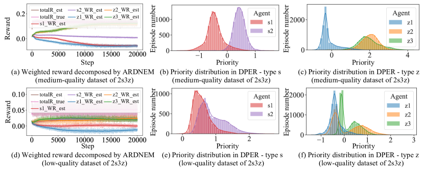
Figure 3: Intermediate results of ARDNEM and DPER modules on 2s3z datasets.

Experiments

In this section, we first introduce the data generation method for agent-wise imbalanced multi-agent datasets in StarCraft II (Samvelyan et al. 2019), multi-agent particle environment (MPE) (Lowe et al. 2017) and multi-agent mujoco (MAmujoco) (Peng et al. 2021). Then, We evaluate our method SIT on these datasets. Finally, we conduct analytical experiments to better illustrate the superiority of our method.

Data Generation for Agent-Wise Imbalanced Multi-Agent Datasets

We construct the agent-wise imbalanced multi-agent datasets based on six maps in StarCraft II (see Table 2 in Appendix C.1) and three maps in MPE (see Table 3 and Figure 5 in Appendix C.1) for discrete control, and two maps in MAmujoco (see Figure 6 in Appendix C.1) for continuous control. In order to obtain diverse behavior policies for generating these imbalanced datasets, we first online train the joint policies based on QMIX (Rashid et al. 2018) (discrete) or FacMAC (Peng et al. 2021) (continuous) in each environment and store them at fixed intervals during the training process. Then, these saved joint policies are deposited into random, medium and expert policy pools according to their episode returns, and the details are elaborated in Table 4, Table 5, Table 6 of Appendix C.2. Since the policy levels among the individual agents during online training are balanced (e.g., the policy level of each individual agent in a medium joint policy is also medium), we can directly sample the required individual behavior policies from different policy pools to generate the agent-wise imbalanced datasets.

For the convenience of expression, each dataset is represented by the type and policy level corresponding to all individual behavior policies. e.g., in ${\rm 3s\_vs_{\_}5z}$ map of StarCraft II, the agent-wise imbalanced multi-agent dataset 100%$[{\rm s_{1}^{r},s_{2}^{m},s_{3}^{e}}]$ indicates that the policy levels of three Stalkers (agents) that generate this data are random, medium and expert, respectively. In practice, since we are interested in non-expert data, we generate low-quality and medium-quality agent-wise imbalanced datasets based on the average episode return for all environments. Each of them contains 10000 trajectories and the detailed configuration is shown in Table 7, Table 8 and Table 9 of Appendix C.3.

Evaluation on Agent-Wise Imbalanced Multi-Agent Datasets

We compare our proposed method against QMIX (discrete), FacMAC (continuous), behavior cloning (BC), multi-agent version of BCQ (Fujimoto, Meger, and Precup 2019) (MABCQ) and CQL (Kumar et al. 2020) (MACQL), and existing start-of-the-art algorithm ICQ (Yang et al. 2021). The value decomposition structure of MABCQ and MACQL follows Yang et al. (2021). Details for baseline implementations are in Appendix B. To better demonstrate the effectiveness of our method, we employ the find-tuned hyper-parameters provided by the authors of BCQ and CQL. Details for experimental configurations are in Appendix D.

Table 1 shows the mean and variance of the episodic return of different algorithms with 5 random seeds on tested maps, where the result corresponding to Behavior represents the average episode return of the offline dataset. It can be found that our method significantly outperforms all baselines in all maps and is even 2x higher than the existing start-of-the-art method ICQ in some maps (e.g., low-quality dataset based on 3s_vs_5z in StarCraft II, medium-quality dataset based on CN_3p1p in MPE and all datasets in MAmujoco), which demonstrates that our method can effectively find and exploit good individual trajectories in agent-wise imbalanced multi-agent datasets to boost the overall performance of multi-agent systems. Note that since the online algorithm QMIX or FacMAC cannot handle the extrapolation error in offline scenarios, its performance is much lower than other methods. We also provide the training curves for all datasets in Appendix E.3 to better understand the strengths of our approach.

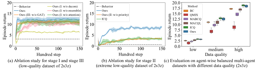
Figure 4: Ablation experiments and the performance on agent-wise balanced datasets.

A Closer Look at SIT

ARDNEM and DPER are two important modules of our SIT. The former is used to estimate individual rewards, and the latter constructs type-wise prioritized experience replays. To better demonstrate the effectiveness of our method, we investigate two questions: 1) Can the learned ARDNEM correctly decompose the global reward into individual rewards? and 2) Can the priority in DPER accurately reflect the quality of individual trajectories? To answer these two questions, we show some intermediate results of our method on medium-quality and low-quality datasets of 2s3z, where the composition of the former is ${\rm 100\%[s_{1}^{r},s_{2}^{e},z_{1}^{r},z_{2}^{e},z_{3}^{e}]}$ and the composition of the latter is ${\rm 50\%[s_{1}^{r},s_{2}^{r},z_{1}^{r},z_{2}^{r},z_{3}^{r}]+50\%[s_{1}^{r},s_{2}^{m},z_{1}^{r},z_{2}^{m},z_{3}^{m}]}$.

Figure 3(a) illustrates the decomposed weighted reward $\hat{r}$, estimated by ARDNEM (denoted as WR in the legend) during training on the medium-quality dataset. We can observe that ${\rm s_{1}}$’s reward (red) is lower than ${\rm s_{2}}$’s reward (violet), and ${\rm z_{1}}$’s reward (blue) is lower than ${\rm z_{2}}$’s reward (orange) and ${\rm z_{3}}$’s reward (green). This decomposition result of ARDNEM agrees with our expectation because all individual trajectories of ${\rm s_{1}}$ and ${\rm z_{1}}$ are generated by random behavior policies, while the individual trajectories of other agents are generated by expert behavior policies. Figure 3(d) illustrates the decomposed weighted reward on the low-quality dataset. Similarly, the comparisons also agree with the intended decomposition we desire to achieve. We further provide the corresponding illustrations for all maps in Appendix E.4, and their decomposition result also matches their data composition (Table 7, Table 8 and Table 9 in Appendix C.3).

Since 2s3z map has two types of agents, we store the individual trajectories of each agent into the corresponding prioritized experience replays by their type. For the medium-quality dataset, Figure 3(b) and Figure 3(c) show the priority distribution of all individual trajectories in each prioritized experience replay. It demonstrates that most individual trajectories of ${\rm s_{1}}$ have lower priority than ${\rm s_{2}}$, while ${\rm z_{1}}$ has lower priority than ${\rm z_{2}}$ and ${\rm z_{3}}$. This comparison is fully consistent with the quality of the individual trajectories, which indicates the priorities in DPER is as intended. Figure 3(e) and Figure 3(f) draw similar conclusions on the low-quality dataset. A deeper look into Figure 3(f) finds that the priority distribution has multiple modals, which indicates that it correctly captures the distribution of the quality even when the variance of the quality is large. e.g., 50% ${\rm z_{2}^{r}}$ + 50% ${\rm z_{2}^{m}}$.

Analytical Experiment

We conduct some analytical experiments to better understand our proposed method. All experiments are evaluated on the low-quality dataset of 2s3z unless otherwise stated.

Ablation study.

Figure 4(a) illustrates the ablation study about stage I and stage III, where ‘(w/o decom)’ represents that the critic of each agent is directly trained based on the total reward without decomposition. ‘(w/o attention)’ represents that the weight $\lambda$ of each estimated reward is always equal to 1 instead of a learnable value. ‘(w/o ensemble)’ removes the ensemble mechanism. ‘(w/o GAT)’ removes the GAT aggregation. The result shows that each part is important in our SIT. To better illustrate the role of priority sampling in stage II, we construct an extreme low-quality dataset based on 2s3z, i.e., ${\rm 99.5\%[s_{1}^{r},s_{2}^{r},z_{1}^{r},z_{2}^{r},z_{3}^{r}]+0.5\%[s_{1}^{r},s_{2}^{m},z_{1}^{r},z_{2}^{m},z_{3}^{m}]}$. The result in Figure 4(b) shows that the priority sampling in stage II plays a key role when the good individual trajectories are sparse in the dataset.

Evaluation on agent-wise balanced multi-agent datasets.

To evaluate the performance of our method on agent-wise balanced multi-agent datasets, we generate datasets with random, medium and expert quality on the 2s3z for evaluation. Figure 4(c) shows our method can achieve similar performance to ICQ on these datasets and is significantly higher than other baselines, which indicates that our method can still work well in agent-wise balanced datasets.

Computational complexity.

According to the experiments, the running time of Stage I (supervised learning) is only 10% of ICQ as it does not contain some complex calculation operations (e.g. CRR trick) during gradient backpropagation. The running time of Stage II is negligible (about 10s) as it only needs the inference of the ARDNEM. The running time of Stage III is similar to ICQ. Almost all experimental maps can be evaluated within 1 GPU day, except 8m, 1c3s5z and 10m_vs_11m maps in StarCraft II which takes 2-3 GPU days.

We also conduct experiments about hyperparameter selection $\alpha,\beta$ and $\eta$. See Appendix E.2 for details.

Conclusion

In this paper, we investigate the diversity of individual trajectories in offline multi-agent datasets and empirically show the current offline algorithms cannot fully exploit the useful knowledge in complex and mixed datasets. e.g., agent-wise imbalanced multi-agent datasets. To address this problem, we propose a novel algorithmic framework called Shared Individual Trajectories (SIT). It can effectively decompose the joint trajectories into individual trajectories, so that the good individual trajectories can be shared among agents to boost the overall performance of multi-agent systems. Extensive experiments on both discrete control (i.e., StarCraft II and MPE) and continuous control (i.e., MAmujoco) demonstrate the effectiveness and superiority of our method in complex and mixed datasets.

Appendix

A. Algorithm

Input: Offline joint dataset $\mathbb{B}$, training epoch of ARDNEM $L_{{{\rm ARDNEM}}}$, training epoch of actor-critic $L_{{{\rm AC}}}$, priority sampling hyperparameter $\alpha$, conservative hyperparameter $\beta$, uncertainty weight $\eta$, network update interval $d$.

1 Initialize ARDNEM $z$ w.r.t. parameters $\psi$, critic networks $Q_{i}$ w.r.t. parameters $\phi_{i}$ and actor networks $\pi_{i}$ w.r.t. parameters $\theta_{i}$ with random parameters.

2 Initialize target critic networks $Q_{i}^{\prime}$.

3 Initialize DPER $\mathbb{B}_{J}=\emptyset$.

// Stage I: learning an ARDNEM.

4 for $l_{{{\rm ARDNEM}}}=1$ to $L_{{{\rm ARDNEM}}}$ do

5       Sample joint trajectories $\{o_{1}^{t,k},a_{1}^{t,k},o_{1}^{t+1,k},\dots,o_{{\rm N}}^{t,k},a_{{\rm N}}^{t,k},o_{{\rm N}}^{t+1,k},s^{t,k},r_{tot}^{t,k}\}$ from $\mathbb{B}$.

6       Train reward decomposition network $z$ with uniform sampling according to $\mathcal{L}_{{\rm MSE}}(\psi)=\mathbb{E}_{{\rm Uniform}(\mathbb{B})}\sum_{m=1}^{M}\frac{1}{M}\left(z(o_{1}^{t,k},a_{1}^{t,k},\dots,o_{{\rm N}}^{t,k},a_{{\rm N}}^{t,k},s^{t,k})-r_{tot}^{t,k}\right)^{2}$.

7      

// Stage II: reconstruct the joint offline dataset into type-wise DPER.

8 for $k=1$ to $K$ do

9       for $i=1$ to $N$ do

10             for $t=1$ to $T$ do

11                   Obtain ensembled weighted reward $\{\lambda_{i,m}^{t,k}r_{i,m}^{t,k}\}^{m=1,\dots,M}$ according to the input $\{o_{i}^{t,k},a_{i}^{t,k},s^{t,k}\}$ and the learned ARDNEM.

12                   Calculate estimated weighted reward $\hat{r}_{i}^{t,k}=\frac{1}{M}\sum_{m=1}^{M}\lambda_{i,m}^{t,k}r_{i,m}^{t,k}$.

13                   Calculate uncertainty $\hat{u}_{i}^{t,k}=\sqrt{\frac{1}{M}\sum_{m=1}^{M}\left(\lambda_{i,m}^{t,k}r_{i,m}^{t,k}-\hat{r}_{i}^{t,k}\right)^{2}}$.

14                   Calculate Monte Carlo return $\hat{g}_{i}^{t,k}=\sum_{t=t^{\prime}}^{T}\gamma^{t-t^{\prime}}\hat{r}_{i}^{t,k}$.

15                  

16            

17      Calculate episode priority $\hat{p}_{i}^{k}=\frac{1}{T}\sum_{t=1}^{T}\hat{g}_{i}^{t,k}$.

18       Reshape episode priority $p_{i}^{k}=\frac{e^{\hat{p}_{i}^{k}/\alpha}}{\sum_{j\in\mathbb{J},k}^{K}e^{\hat{p}_{j}^{k}/\alpha}}$.

19       Store the individual trajectory $\{\{o_{i}^{t,k},a_{i}^{t,k},o_{i}^{t+1,k},\bm{o_{-i}}^{t,k},\hat{r}_{i}^{t,k},\hat{u}_{i}^{t,k}\}^{i=1,\dots,N.t=1,\dots,T},p_{i}^{k}\}$ in DPER $\mathbb{B}_{J}$ according to the agent type $J$.

// Stage III: conservative policy training with GAT-based critic.

20 for $l_{{{\rm AC}}}=1$ to $L_{{{\rm AC}}}$ do

21       Sample the individual trajectory from $\mathbb{B}_{J}$ with priority-based sampling strategy $P_{J}$ for each agent $i$.

22       Train critic networks $Q_{i}$ according to $\mathcal{L}_{{\rm critic}}(\phi_{i})=\mathbb{E}_{P_{J}\left(\mathbb{B}_{J}\right)}\left[\frac{\eta}{\hat{u}_{i(j)}^{t,k}}\left(\hat{r}_{i(j)}^{t,k}+\gamma Q_{i}^{\prime}\left(\tau_{i(j)}^{t+1,k},a_{i(j)}^{t+1,k},\bm{o_{-i(-j)}}^{t+1,k}\right)-Q_{i}\left(\tau_{i(j)}^{t,k},a_{i(j)}^{t,k},\bm{o_{-i(-j)}}^{t,k}\right)\right)^{2}\right]$.

23       Train actor networks $\pi_{i}$ according to $\mathcal{L}_{{\rm actor}}(\theta_{i})=\mathbb{E}_{P_{J}\left(\mathbb{B}_{J}\right)}\left[-\frac{\eta}{\hat{u}_{i(j)}^{t,k}}\frac{e^{Q_{i}\left(\tau_{i(j)}^{t,k},a_{i(j)}^{t,k},\bm{o_{-i(-j)}}^{t,k}\right)/\beta}}{Z}\left.Q_{i}\left(\tau_{i(j)}^{t,k},a,\bm{o_{-i(-j)}}^{t,k}\right)\right|_{a=a_{i(j)}^{t,k}}\right]$.

24       if $l_{{{\rm AC}}}$ mod $d=0$ then

25             Update target networks: $Q_{i}^{\prime}=Q_{i}$.

26            

27      

Algorithm 1 Shared Individual Trajectories (SIT)

B. Baseline implementations

BC. Each agent policy $\pi_{i}$ w.r.t. parameters $\theta_{i}$ is optimized by the following loss

$$\mathcal{L}_{\rm BC}(\theta_{i})=\mathbb{E}_{\tau_{i},a_{i}\sim\mathbb{B}}[-\log(\pi_{i}(a_{i}\mid\tau_{i}))].$$ (11)

MABCQ. Suppose the mixer network $Q$ w.r.t. parameters $\phi$, the individual $Q$ networks $Q_{i}$ w.r.t. parameters $\phi_{i}$, the behavior policies $\mu_{i}$ w.r.t. parameters $\theta_{i}$. We first train behavior policies $\mu_{i}$ by behavior cloning, then the agent networks is trained by the following loss

$$\begin{aligned} \mathcal{L}_{\rm BCQ}(\phi,\phi_{i})&=\mathbb{E}_{\bm{\tau},\bm{a},r,\bm{\tau^{\prime}}\sim\mathbb{B}}\left[\left(r+\gamma\max_{\tilde{\bm{a}}^{[j]}}Q^{\prime}(\bm{\tau^{\prime}},\tilde{\bm{a}}^{[j]})-Q(\bm{\tau},\bm{a})\right)^{2}\right]\\ &\qquad\quad\quad\tilde{\bm{a}}^{[j]}=\bm{a}^{[j]}+\xi(\bm{\tau},\bm{a}^{[j]})\end{aligned},$$ (12)

where $Q(\bm{\tau},\bm{a})=w_{i}Q_{i}(\tau_{i},a_{i})+b$ and $\xi(\bm{\tau},\bm{a}^{[j]})$ denotes the perturbation model, which is decomposed as $\xi_{i}(\tau_{i},a_{i}^{[j]})$. If $\frac{a_{i}^{[j]}\sim\mu_{i}(\tau_{i})}{\max\{a_{i}^{[j]}\sim\mu_{i}(\tau_{i})\}_{j=1}^{m}}\leq\zeta$ in agent $i$, $a_{i}^{[j]}$ is considered an unfamiliar action and $\xi^{i}(\tau^{i},a_{i}^{[j]})$ will mask $a_{i}^{[j]}$ in maximizing $Q_{i}$-value operation.

MACQL. Suppose the mixer network $Q$ w.r.t. parameters $\phi$, the individual $Q$ networks $Q_{i}$ w.r.t. parameters $\phi_{i}$, then the agent networks is trained by the following loss

$$\mathcal{L}_{\rm CQL}(\phi,\phi_{i}) =\beta_{\rm CQL}\mathbb{E}_{\tau_{i},a_{i},\bm{\tau},\bm{a}\sim\mathbb{B}}\left[\sum_{i}\log\sum_{a_{i}}\exp(w_{i}Q_{i}(\tau_{i},a_{i})+b)-\mathbb{E}_{\bm{a}\sim\bm{\mu}(\bm{a}\mid\bm{\tau})}[Q(\bm{\tau},\bm{a})]\right]$$ (13)

$$\qquad\qquad\qquad\qquad\qquad\qquad\qquad\qquad+\frac{1}{2}\mathbb{E}_{\bm{\tau}\sim\mathbb{B},\bm{a}\sim\bm{\mu}(\bm{a}\mid\bm{\tau})}\left[\left(y_{\rm CQL}-Q(\bm{\tau},\bm{a})\right)^{2}\right],$$

where $y_{\rm CQL}$ is calculated based on $n$-step off-policy estimation (e.g., Tree Backup algorithm).

ICQ. Suppose the centralized critic network $Q$ w.r.t. parameters $\phi$, the individual critic networks $Q_{i}$ w.r.t. parameters $\phi_{i}$, the individual policies $\pi_{i}$ w.r.t. parameters $\theta_{i}$, then the actor-critic is trained by the following loss

$$\mathcal{L}_{{\rm actor}}(\theta_{i}) =\mathbb{E}_{\tau_{i},a_{i}\sim\mathbb{B}}\left[-\frac{1}{Z_{i}}\log(\pi_{i}(a_{i}\mid\tau_{i}))\exp\left(\frac{w_{i}Q_{i}(\tau_{i},a_{i})}{\beta_{{\rm ICQ}}}\right)\right]$$ (14)

$$\mathcal{L}_{{\rm critic}}(\phi,\phi_{i}) =\mathbb{E}_{\bm{\tau},\bm{a},r,\bm{\tau^{\prime}},\bm{a^{\prime}}\sim\mathbb{B}}\left[\sum_{t\geq 0}(\gamma\lambda_{{\rm ICQ}})^{t}\left[r+\gamma\frac{\exp\left(\frac{1}{\beta_{{\rm ICQ}}}Q(\bm{\tau^{\prime}},\bm{a^{\prime}})\right)}{Z}Q(\bm{\tau^{\prime}},\bm{a^{\prime}})-Q(\bm{\tau},\bm{a})\right]\right]^{2},$$

where $Q(\bm{\tau},\bm{a})=w_{i}Q_{i}(\tau_{i},a_{i})+b$ represents the linear mixer of the centralized critic network.

C. Environment and offline dataset information

C.1 Environment information

In this paper, we construct the agent-wise imbalanced multi-agent datasets based on six maps in StarCraft II, three modified maps for partially observable settings in the multi-agent particle environment (MPE) and two maps in multi-agent mujoco (MAmujoco). To better understand our experiments, we give a brief introduction to these environments.

Maps	Controlled ally agents	Built-in enemy agents	Difficulties
2s_vs_1sc	2 Stalkers	1 Spine Crawler	Super Hard
3s_vs_5z	3 Stalkers	5 Zealots	Super Hard
2s3z	2 Stalkers & 3 Zealots	2 Stalkers & 3 Zealots	Super Hard
8m	8 Marines	8 Marines	Super Hard
1c3s5z	1 Colossus, 3 Stalkers & 5 Zealots	1 Colossus, 3 Stalkers & 5 Zealots	Super Hard
10m_vs_11m	10 Marines	11 Marines	Super Hard

Table 2: The information of test maps on StarCraft II.

StarCraft II.

StarCraftII micromanagement aims to accurately control the individual units and complete cooperation tasks. In this environment, each enemy unit is controlled by the built-in AI while each allied unit is controlled by a learned policy. The local observation of each agent contains the following attributes for both allied and enemy units within the sight range: ${\rm distance}$, ${\rm relative\_x}$, ${\rm relative\_y}$, ${\rm health}$, ${\rm shield}$, and ${\rm unit\_type}$. The action space of each agent includes: ${\rm noop}$, ${\rm move[direction]}$, ${\rm attack[enemyid]}$, and ${\rm stop}$. Under the control of these actions, each agent can move and attack in various maps. The reward setting is based on the hit-point damage dealt on the enemy units, together with special bonuses for killing the enemy units and winning the battle. In our experiments, we choose 2s_vs_1sc, 3s_vs_5z, 2s3z, 8m, 1c3s5z and 10m_vs_11m for evaluation, and more detailed information about these maps is shown in Table 2.

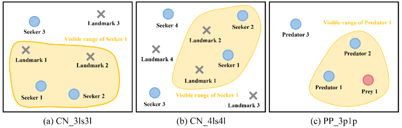
Figure 5: Three modified maps for partially observable settings in MPE.

Maps	Controlled agents	Targets	Visible agents	Visible targets
CN_3ls3l (Cooperative navigation)	3 Landmark Seekers	3 Landmarks	1 Landmark Seeker	2 Landmarks
CN_4ls4l (Cooperative navigation)	4 Landmark Seekers	4 Landmarks	1 Landmark Seeker	2 Landmarks
PP_3p1p (Predator-prey)	3 Predators	1 Prey	1 Predator	1 Prey

Table 3: The information of test maps on MPE.

Multi-agent particle environment (MPE).

MPE is a common benchmark that contains various multi-agent games. In this paper, we choose the discrete version of cooperative navigation (CN) and predator-prey (PP) for evaluation. In CN task, landmark seeks (agents) must cooperate through physical actions to reach a set of landmarks without colliding with each other. In PP task, some slower cooperating predators must chase the faster prey and avoid collisions in a randomly generated environment. We set the prey as a heuristic agent whose movement direction is always away from the nearest predator. Note that in the original MPE environment, each agent can directly observe the global information of the environment. However, we modify the environment to the partially observable setting, a more challenging and practical setting, thus we reset the local observation of the agents in each map as shown in Figure 5 and Table 3.

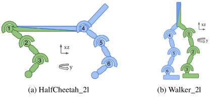
Figure 6: Two maps in MAmujoco.

Multi-agent mujoco (MAmujoco).

MAmujoco is a novel benchmark for continuous cooperative multi-agent robotic control. Starting from the popular single-agent robotic mujoco (Todorov, Erez, and Tassa 2012) control suite included with OpenAI Gym (Brockman et al. 2016). Each agent’s action space in MAmujoco is given by the joint action space over all motors controllable by that agent. As shown in Figure 6, we select HalfCheetah_2l and Walker_2l maps with 200 termination steps for evaluation. In these two maps, each agent can control joints of one color. For example, the agent corresponding to the green partition in HalfCheetah_2l (Figure 6(a)) consists of three joints (joint ids 1, 2, and 3) and four adjacent body segments. Each joint has an action space $[-1,1]$, so the action space for each agent is a 3-dimensional vector with each entry in $[-1,1]$.

C.2 Policy pools for each environments

In order to obtain diverse behavior policies for generating agent-wise imbalanced multi-agent datasets, we first online train the joint policies based on QMIX (Rashid et al. 2018) (discrete) or FacMAC (Peng et al. 2021) (continuous) in each environment and store them at fixed intervals during the training process. Then, these saved joint policies are deposited into random, medium and expert policy pools according to their episode returns. Table 4, Table 5 and Table 6 show the episode return corresponding to different policy pools in each map, where ‘Episode return range’ is determined by fully random policies and the best policies trained by QMIX or FacMAC. After these policy pools are constructed, we can directly sample the required individual behavior policies from different policy pools to generate the agent-wise imbalanced multi-agent datasets.

Maps	Random pools	Medium pools	Expert pools	Episode return range
2s_vs_1sc	0$\sim$6	6$\sim$14	14$\sim$20	0$\sim$20
3s_vs_5z	0$\sim$6	6$\sim$14	14$\sim$20	0$\sim$20
2s3z	0$\sim$6	6$\sim$14	14$\sim$20	0$\sim$20
8m	0$\sim$6	6$\sim$14	14$\sim$20	0$\sim$20
1c3s5z	0$\sim$6	6$\sim$14	14$\sim$20	0$\sim$20
10m_vs_11m	0$\sim$6	6$\sim$14	14$\sim$20	0$\sim$20

Table 4: Episode return of different policy pools in StarCraft II.

Maps	Random pools	Medium pools	Expert pools	Episode return range
CN_3ls3l	-174.41$\sim$-133.28	-133.28$\sim$-78.44	-78.44$\sim$-37.32	-174.41$\sim$-37.32
CN_4ls4l	-288.89$\sim$-214.47	-214.47$\sim$-115.24	-115.24$\sim$-40.81	-288.89$\sim$-40.81
PP_3p1p	-306.57$\sim$-231.08	-231.08$\sim$-130.44	-130.44$\sim$-54.96	-306.57$\sim$-54.96

Table 5: Episode return of different policy pools in MPE.

Maps	Random pools	Medium pools	Expert pools	Episode return range
HalfCheetah_2l	-203.47$\sim$-69.42	-69.42$\sim$64.63	64.63$\sim$198.70	-203.47$\sim$198.70
Walker_2l	-74.51$\sim$27.35	27.35$\sim$129.21	129.21$\sim$231.09	-74.51$\sim$231.09

Table 6: Episode return of different policy pools in MAmujoco.

C.3 Data components of agent-wise imbalanced offline multi-agent datasets

After the policy pools are ready, we sample the individual behavior policies from these pools according to the data composition in Table 7, Table 8 and Table 9, and generate agent-wise imbalanced offline datasets. Note that since we are interested in non-expert data, We mainly generate two types of datasets. i.e., low-quality and medium-quality datasets.

	Maps	Components	Average episode return	Episode number
Low Quality	2s_vs_1sc	${\rm 50\%[s_{1}^{r},s_{2}^{r}]+}$ ${\rm 50\%[s_{1}^{r},s_{2}^{m}]}$	2.84	10000
	3s_vs_5z	${\rm 50\%[s_{1}^{r},s_{2}^{r},s_{3}^{r}]+}$ ${\rm 50\%[s_{1}^{r},s_{2}^{r},s_{3}^{m}]}$	2.94	10000
	2s3z	${\rm 50\%[s_{1}^{r},s_{2}^{r},z_{1}^{r},z_{2}^{r},z_{3}^{r}]+}$ ${\rm 50\%[s_{1}^{r},s_{2}^{m},z_{1}^{r},z_{2}^{m},z_{3}^{m}]}$	3.24	10000
	8m	${\rm 50\%[m_{1}^{r},m_{2}^{r},m_{3}^{r},m_{4}^{r},m_{5}^{r},m_{6}^{r},m_{7}^{r},m_{8}^{r}]+}$ ${\rm 50\%[m_{1}^{r},m_{2}^{r},m_{3}^{r},m_{4}^{r},m_{5}^{r},m_{6}^{r},m_{7}^{r},m_{8}^{m}]}$	3.10	10000
	1c3s5z	${\rm 50\%[c_{1}^{r},s_{1}^{r},s_{2}^{r},s_{3}^{r},z_{1}^{r},z_{2}^{r},z_{3}^{r},z_{4}^{r},z_{5}^{r}]+}$ ${\rm 50\%[c_{1}^{m},s_{1}^{r},s_{2}^{r},s_{3}^{m},z_{1}^{r},z_{2}^{r},z_{3}^{r},z_{4}^{r},z_{5}^{m}]}$	5.56	10000
	10m_vs_11m	${\rm 50\%[m_{1}^{r},m_{2}^{r},m_{3}^{r},m_{4}^{r},m_{5}^{r},m_{6}^{r},m_{7}^{r},m_{8}^{r},m_{9}^{r},m_{10}^{r}]+}$ ${\rm 50\%[m_{1}^{r},m_{2}^{r},m_{3}^{m},m_{4}^{m},m_{5}^{m},m_{6}^{m},m_{7}^{m},m_{8}^{m},m_{9}^{m},m_{10}^{m}]}$	3.82	10000
Medium Quality	2s_vs_1sc	${\rm 100\%[s_{1}^{r},s_{2}^{e}]}$	9.86	10000
	3s_vs_5z	${\rm 100\%[s_{1}^{r},s_{2}^{r},s_{3}^{e}]}$	7.06	10000
	2s3z	${\rm 100\%[s_{1}^{r},s_{2}^{e},z_{1}^{r},z_{2}^{e},z_{3}^{e}]}$	7.04	10000
	8m	${\rm 100\%[m_{1}^{r},m_{2}^{e},m_{3}^{e},m_{4}^{e},m_{5}^{e},m_{6}^{e},m_{7}^{e},m_{8}^{e}]}$	9.85	10000
	1c3s5z	${\rm 100\%[c_{1}^{e},s_{1}^{r},s_{2}^{r},s_{3}^{e},z_{1}^{r},z_{2}^{r},z_{3}^{r},z_{4}^{r},z_{5}^{e}]}$	10.31	10000
	10m_vs_11m	${\rm 100\%[m_{1}^{r},m_{2}^{e},m_{3}^{e},m_{4}^{e},m_{5}^{e},m_{6}^{e},m_{7}^{e},m_{8}^{e},m_{9}^{e},m_{10}^{e}]}$	9.23	10000

Table 7: Data components of agent-wise imbalanced offline multi-agent datasets in StarCraft II.

	Maps	Components	Average episode return	Episode number
Random Quality	CN_3ls3l	${\rm 50\%[ls_{1}^{r},ls_{2}^{r},ls_{3}^{r}]+}$ ${\rm 50\%[ls_{1}^{r},ls_{2}^{r},ls_{3}^{m}]}$	-157.70	10000
	CN_4ls4l	${\rm 50\%[ls_{1}^{r},ls_{2}^{r},ls_{3}^{r},ls_{4}^{r}]+}$ ${\rm 50\%[ls_{1}^{r},ls_{2}^{r},ls_{3}^{r},ls_{4}^{m}]}$	-278.40	10000
	PP_3p1p	${\rm 50\%[p_{1}^{r},p_{2}^{r},p_{3}^{r}]+}$ ${\rm 50\%[p_{1}^{r},p_{2}^{r},p_{3}^{m}]}$	-249.58	10000
Medium Quality	CN_3ls3l	${\rm 100\%[ls_{1}^{r},ls_{2}^{m},ls_{3}^{e}]}$	-107.46	10000
	CN_4ls4l	${\rm 100\%[ls_{1}^{r},ls_{2}^{r},ls_{3}^{e},ls_{4}^{e}]}$	-166.26	10000
	PP_3p1p	${\rm 100\%[p_{1}^{r},p_{2}^{m},p_{3}^{e}]}$	-155.46	10000

Table 8: Data components of agent-wise imbalanced offline multi-agent datasets in MPE.

	Maps	Components	Average episode return	Episode number
Random Quality	HalfCheetah_2l	${\rm 100\%[l_{1}^{m},l_{2}^{r}]}$	-110.52	10000
	Walker_2l	${\rm 100\%[l_{1}^{r},l_{2}^{m}]}$	-21.67	10000
Medium Quality	HalfCheetah_2l	${\rm 100\%[l_{1}^{r},l_{2}^{e}]}$	41.79	10000
	Walker_2l	${\rm 100\%[l_{1}^{r},l_{2}^{e}]}$	71.68	10000

Table 9: Data components of agent-wise imbalanced offline multi-agent datasets in MAmujoco.

D. Experimental configurations

D.1 Hardware configurations

In all experiments, the GPU is NVIDIA A100 and the CPU is AMD EPYC 7H12 64-Core Processor.

D.2 Hyperparameters

In our proposed algorithmic framework SIT, we first train ARDNEM with the hyperparameters shown in Figure 10, then take the last checkpoint to construct type-wise DPER, and finally use the hyperparameters shown in Figure 11 to train the agent policies. To ensure a fair comparison, other baselines also share most hyperparameters with ours during agent training as shown in Figure 11.

Hyperparameter	Value
Learning rate	$1\times 10^{-4}$
Optimizer	RMS
Training epoch	20000
Gradient clipping	10
Reward network dimension	64
Attention hidden dimension	64
Activation function	ReLU
Batch size	32
Replay buffer size	$1.0\times 10^{4}$
Ensemble number	5

Table 10: Hyperparameters sheet for ARDNEM learning

Hyperparameter	Value
Shared
Agent network learning rate	$5\times 10^{-4}$
Optimizer	RMS
Discount factor	0.99
Training epoch	15000
Parameters update interval	100
Gradient clipping	10
Mixer/Critic hidden dimension	32
RNN hidden dimension	64
Activation function	ReLU
Batch size	32
Replay buffer size	$1.0\times 10^{4}$
MABCQ
$\zeta$	0.3
MACQL
$\beta_{\rm CQL}$	2.0
ICQ
Critic network learning rate	$1\times 10^{-4}$
$\beta_{\rm ICQ}$	0.1
$\lambda_{\rm ICQ}$	0.8
Ours
Critic network learning rate	$1\times 10^{-4}$
$\alpha$	0.2
$\beta$	0.1
$\eta$	1
Rescaled priority range	[0,20]

Table 11: Hyperparameters sheet for agent learning

E. Experiments

E.1 Reward decomposition network with the monotonic nonlinear constraint (MNC).

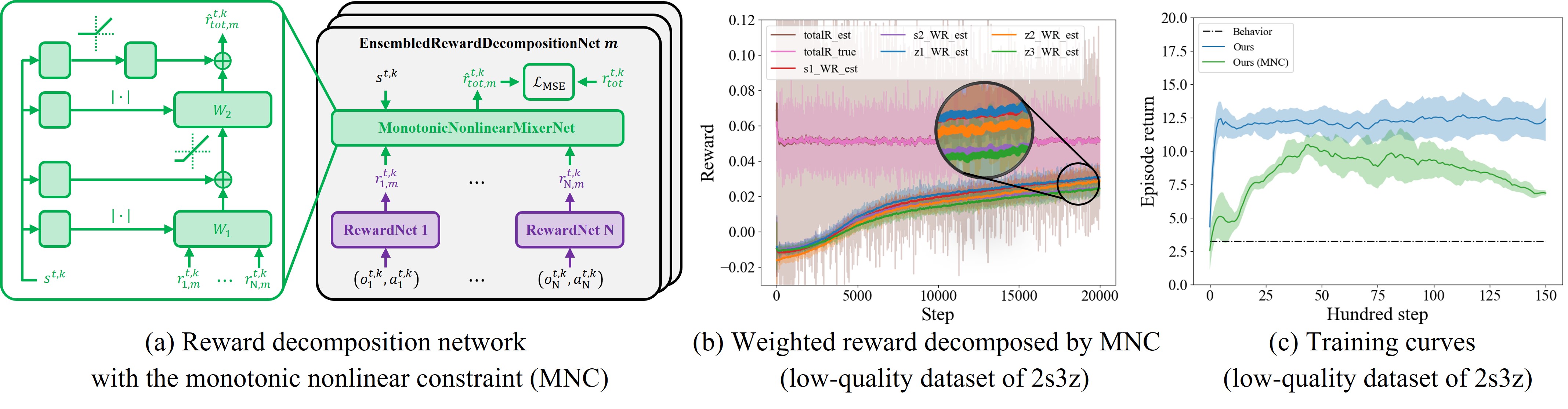
Figure 7: Experiment about reward decomposition network with the monotonic nonlinear constraint (MNC).

In our SIT, we propose an attention-based reward decomposition network in the stage I. A natural alternative is the decomposition module with monotonic nonlinear constraint (MNC), similar to QMIX (Rashid et al. 2018). Specifically, we only need to use the hypernetwork shown in Figure 7(a), so that the total reward $r_{tot}$ and the individual reward $r_{i}$ satisfy the following relationship to achieve reward decomposition

$$\frac{\partial r_{tot}}{\partial r_{i}}\geq 0,~{}\forall i\in N.$$ (15)

Figure 7(b) shows the reward decomposition result of MNC. We can observe there are two problems with the decomposition result. 1) The gap between individual rewards is small, so the quality of the trajectory cannot be well distinguished. 2) More importantly, the reward decomposition result is incorrect. According to the data composition of low-quality dataset of 2s3z. i.e., Table 7. we expect s1 (red)$<$s2 (violet), z1 (blue)$<$z2 (orange), z3 (green), Figure 7(b) does not match this expectation. Instead, the decomposition result of our SIT is as intended. i.e., Figure 3(d). Therefore, policy learning with MNC-decomposed rewards cannot achieve the satisfactory result, as shown in Figure 7(c).

E.2 Hyperparameter selection $\alpha,\beta$ and $\eta$.

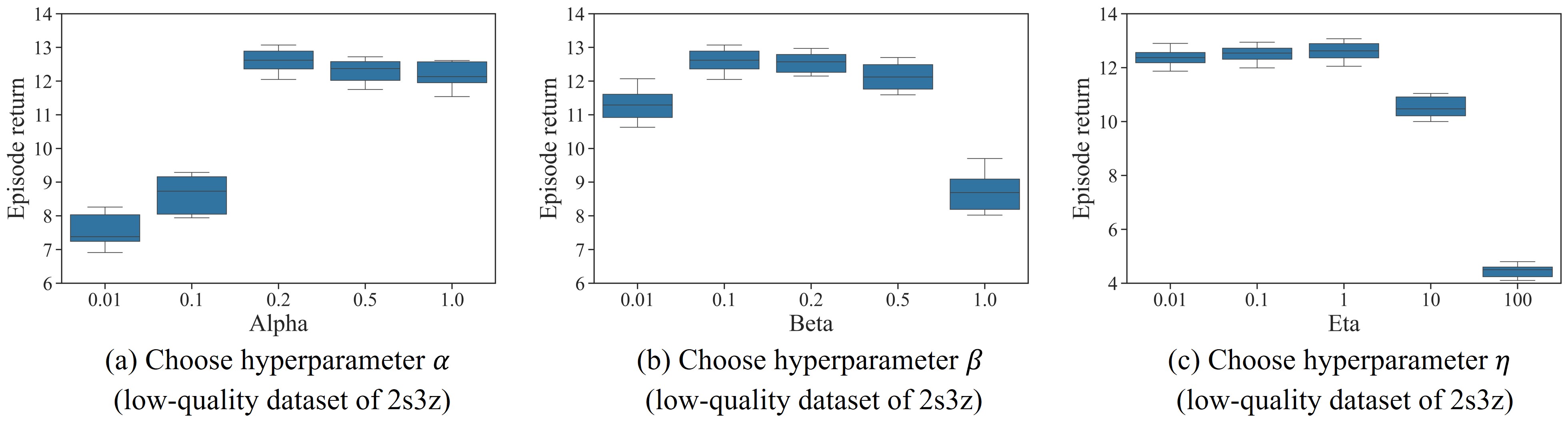
Figure 8: Hyperparameter selection.

The hyperparameter $\alpha$ in Equation (7) determines how much prioritization is used during sampling training data. If $\alpha\rightarrow 0$, it means we only sample the highest quality individual trajectory, while $\alpha\rightarrow\infty$ corresponds to the uniform sampling. The hyperparameter $\beta$ in Equation (10) controls how conservative the policy update is used during training. If $\beta\rightarrow 0$, there are no constraints on policy updates, while $\beta\rightarrow\infty$ results in that agent learning is equivalent to behavior cloning. The hyperparameter $\eta$ in Equation (9) and Equation (10) controls the importance weight of the uncertainty on actor-critic learning. In all experiments, we choose $\alpha=0.2$, $\beta=0.1$ and $\eta=1$ according to Figure 8.

E.3 Training curves

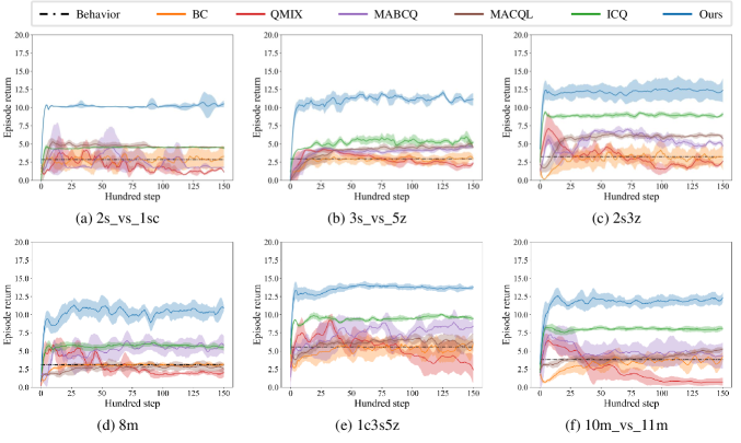
Figure 9: The performance of different algorithms on the low-quality datasets (StarCraft II)

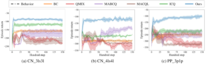
Figure 10: The performance of different algorithms on the low-quality datasets (MPE)

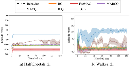
Figure 11: The performance of different algorithms on the low-quality datasets (MAmujoco)

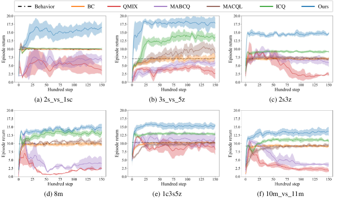
Figure 12: The performance of different algorithms on the medium-quality datasets (StarCraft II)

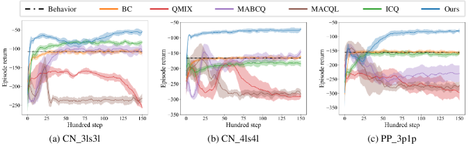
Figure 13: The performance of different algorithms on the medium-quality datasets (MPE)

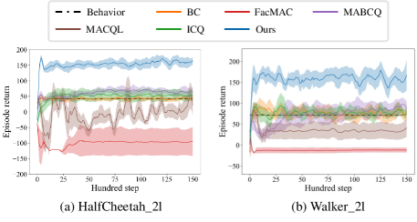
Figure 14: The performance of different algorithms on the medium-quality datasets (MAmujoco)

E.4 Decomposed weighted individual reward

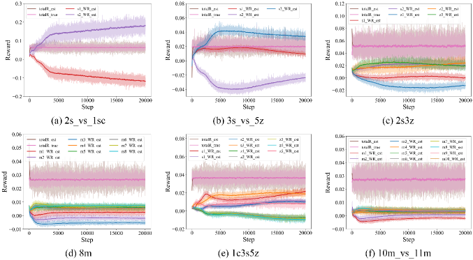
Figure 15: Decomposed weighted individual reward on the low-quality datasets (StarCraft II)

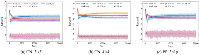
Figure 16: Decomposed weighted individual reward on the low-quality datasets (MPE)

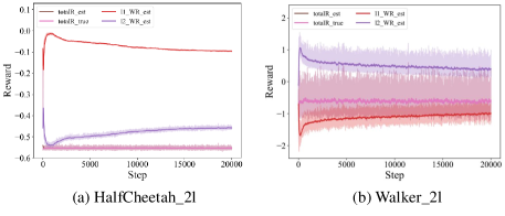
Figure 17: Decomposed weighted individual reward on the low-quality datasets (MAmujoco)

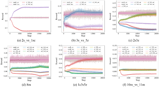
Figure 18: Decomposed weighted individual reward on the medium-quality datasets (StarCraft II)

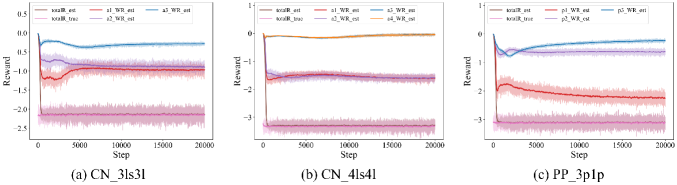
Figure 19: Decomposed weighted individual reward on the medium-quality datasets (MPE)

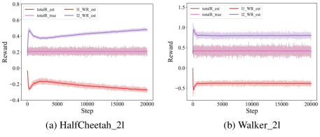
Figure 20: Decomposed weighted individual reward on the medium-quality datasets (MAmujoco)

References

- Bazzan (2009) Bazzan, A. L. 2009. Opportunities for multiagent systems and multiagent reinforcement learning in traffic control. Autonomous Agents and Multi-Agent Systems, 18(3): 342–375.
- Brockman et al. (2016) Brockman, G.; Cheung, V.; Pettersson, L.; Schneider, J.; Schulman, J.; Tang, J.; and Zaremba, W. 2016. Openai gym. arXiv preprint arXiv:1606.01540.
- Chang, Ho, and Kaelbling (2003) Chang, Y.-H.; Ho, T.; and Kaelbling, L. 2003. All learning is local: Multi-agent learning in global reward games. In NeurIPS.
- Christianos, Schäfer, and Albrecht (2020) Christianos, F.; Schäfer, L.; and Albrecht, S. 2020. Shared experience actor-critic for multi-agent reinforcement learning. In NeurIPS.
- Chua et al. (2018) Chua, K.; Calandra, R.; McAllister, R.; and Levine, S. 2018. Deep reinforcement learning in a handful of trials using probabilistic dynamics models. In NeurIPS.
- Foerster et al. (2017) Foerster, J.; Nardelli, N.; Farquhar, G.; Afouras, T.; Torr, P. H.; Kohli, P.; and Whiteson, S. 2017. Stabilising experience replay for deep multi-agent reinforcement learning. In ICML.
- Fujimoto and Gu (2021) Fujimoto, S.; and Gu, S. S. 2021. A minimalist approach to offline reinforcement learning. In NeurIPS.
- Fujimoto, Meger, and Precup (2019) Fujimoto, S.; Meger, D.; and Precup, D. 2019. Off-policy deep reinforcement learning without exploration. In ICML.
- Garcıa (2015) Garcıa, J. 2015. A comprehensive survey on safe reinforcement learning. Journal of Machine Learning Research, 16(1): 1437–1480.
- Gronauer (2022) Gronauer, S. 2022. Multi-agent deep reinforcement learning: a survey. Artificial Intelligence Review, 55(2): 895–943.
- Gulcehre et al. (2021) Gulcehre, C.; Colmenarejo, S. G.; Wang, Z.; Sygnowski, J.; Paine, T.; Zolna, K.; Chen, Y.; Hoffman, M.; Pascanu, R.; and de Freitas, N. 2021. Regularized behavior value estimation. In arXiv preprint arXiv:2103.09575.
- Hüttenrauch et al. (2019) Hüttenrauch, M.; Adrian, S.; Neumann, G.; et al. 2019. Deep reinforcement learning for swarm systems. Journal of Machine Learning Research, 20(54): 1–31.
- Jiang and Lu (2021a) Jiang, J.; and Lu, Z. 2021a. Offline decentralized multi-agent reinforcement learning. In arXiv preprint arXiv:2108.01832.
- Jiang and Lu (2021b) Jiang, J.; and Lu, Z. 2021b. Online Tuning for Offline Decentralized Multi-Agent Reinforcement Learning. In openreview.
- Kumar et al. (2019) Kumar, A.; Fu, J.; Soh, M.; Tucker, G.; and Levine, S. 2019. Stabilizing off-policy q-learning via bootstrapping error reduction. In NeurIPS.
- Kumar et al. (2020) Kumar, A.; Zhou, A.; Tucker, G.; and Levine, S. 2020. Conservative q-learning for offline reinforcement learning. In NeurIPS.
- Li et al. (2021) Li, J.; Kuang, K.; Wang, B.; Liu, F.; Chen, L.; Wu, F.; and Xiao, J. 2021. Shapley counterfactual credits for multi-agent reinforcement learning. In SIGKDD.
- Lin (1992) Lin, L.-J. 1992. Self-improving reactive agents based on reinforcement learning, planning and teaching. Machine learning, 8(3): 293–321.
- Lowe et al. (2017) Lowe, R.; Wu, Y. I.; Tamar, A.; Harb, J.; Pieter Abbeel, O.; and Mordatch, I. 2017. Multi-agent actor-critic for mixed cooperative-competitive environments. In Advances in neural information processing systems.
- Meng et al. (2021) Meng, L.; Wen, M.; Yang, Y.; Le, C.; Li, X.; Zhang, W.; Wen, Y.; Zhang, H.; Wang, J.; and Xu, B. 2021. Offline Pre-trained Multi-Agent Decision Transformer: One Big Sequence Model Conquers All StarCraftII Tasks. In arXiv preprint arXiv:2112.02845.
- Nair et al. (2020) Nair, A.; Gupta, A.; Dalal, M.; and Levine, S. 2020. Awac: Accelerating online reinforcement learning with offline datasets. In arXiv preprint arXiv:2006.09359.
- Oh et al. (2016) Oh, J.; Chockalingam, V.; Lee, H.; et al. 2016. Control of memory, active perception, and action in minecraft. In ICML.
- Oh et al. (2020) Oh, Y.; Lee, K.; Shin, J.; Yang, E.; and Hwang, S. J. 2020. Learning to Sample with Local and Global Contexts in Experience Replay Buffer. In ICLR.
- Oliehoek and Amato (2016) Oliehoek, F. A.; and Amato, C. 2016. A concise introduction to decentralized POMDPs. Springer.
- Omidshafiei et al. (2017) Omidshafiei, S.; Pazis, J.; Amato, C.; How, J. P.; and Vian, J. 2017. Deep decentralized multi-task multi-agent reinforcement learning under partial observability. In ICML.
- Osband et al. (2016) Osband, I.; Blundell, C.; Pritzel, A.; and Van Roy, B. 2016. Deep exploration via bootstrapped DQN. In NeurIPS.
- Palmer et al. (2018) Palmer, G.; Tuyls, K.; Bloembergen, D.; and Savani, R. 2018. Lenient Multi-Agent Deep Reinforcement Learning. In AAMAS.
- Peng et al. (2021) Peng, B.; Rashid, T.; Schroeder de Witt, C.; Kamienny, P.-A.; Torr, P.; Böhmer, W.; and Whiteson, S. 2021. Facmac: Factored multi-agent centralised policy gradients. In NeurIPS.
- Rashid et al. (2018) Rashid, T.; Samvelyan, M.; Schroeder, C.; Farquhar, G.; Foerster, J.; and Whiteson, S. 2018. Qmix: Monotonic value function factorisation for deep multi-agent reinforcement learning. In ICML.
- Samvelyan et al. (2019) Samvelyan, M.; Rashid, T.; Schroeder de Witt, C.; Farquhar, G.; Nardelli, N.; Rudner, T. G.; Hung, C.-M.; Torr, P. H.; Foerster, J.; and Whiteson, S. 2019. The StarCraft Multi-Agent Challenge. In AAMAS.
- Schaul et al. (2016) Schaul, T.; Quan, J.; Antonoglou, I.; and Silver, D. 2016. Prioritized Experience Replay. In ICLR.
- Shalev-Shwartz, Shammah, and Shashua (2016) Shalev-Shwartz, S.; Shammah, S.; and Shashua, A. 2016. Safe, multi-agent, reinforcement learning for autonomous driving. In arXiv preprint arXiv:1610.03295.
- Sunehag et al. (2018) Sunehag, P.; Lever, G.; Gruslys, A.; Czarnecki, W. M.; Zambaldi, V. F.; Jaderberg, M.; Lanctot, M.; Sonnerat, N.; Leibo, J. Z.; Tuyls, K.; et al. 2018. Value-Decomposition Networks For Cooperative Multi-Agent Learning Based On Team Reward. In AAMAS.
- Todorov, Erez, and Tassa (2012) Todorov, E.; Erez, T.; and Tassa, Y. 2012. Mujoco: A physics engine for model-based control. In 2012 IEEE/RSJ international conference on intelligent robots and systems, 5026–5033. IEEE.
- Veličković et al. (2018) Veličković, P.; Cucurull, G.; Casanova, A.; Romero, A.; Liò, P.; and Bengio, Y. 2018. Graph Attention Networks. In ICLR.
- Wang et al. (2020a) Wang, H.-n.; Liu, N.; Zhang, Y.-y.; Feng, D.-w.; Huang, F.; Li, D.-s.; and Zhang, Y.-m. 2020a. Deep reinforcement learning: a survey. Frontiers of Information Technology & Electronic Engineering.
- Wang et al. (2020b) Wang, W.; Yang, T.; Liu, Y.; Hao, J.; Hao, X.; Hu, Y.; Chen, Y.; Fan, C.; and Gao, Y. 2020b. Action semantics network: Considering the effects of actions in multiagent systems. In ICLR.
- Wang et al. (2020c) Wang, Z.; Novikov, A.; Zolna, K.; Merel, J. S.; Springenberg, J. T.; Reed, S. E.; Shahriari, B.; Siegel, N.; Gulcehre, C.; Heess, N.; et al. 2020c. Critic regularized regression. In NeurIPS.
- Wu, Tucker, and Nachum (2019) Wu, Y.; Tucker, G.; and Nachum, O. 2019. Behavior regularized offline reinforcement learning. In arXiv preprint arXiv:1911.11361.
- Yang et al. (2020a) Yang, Y.; Hao, J.; Chen, G.; Tang, H.; Chen, Y.; Hu, Y.; Fan, C.; and Wei, Z. 2020a. Q-value path decomposition for deep multiagent reinforcement learning. In ICML.
- Yang et al. (2020b) Yang, Y.; Hao, J.; Liao, B.; Shao, K.; Chen, G.; Liu, W.; and Tang, H. 2020b. Qatten: A general framework for cooperative multiagent reinforcement learning. In arXiv preprint arXiv:2002.03939.
- Yang et al. (2021) Yang, Y.; Ma, X.; Chenghao, L.; Zheng, Z.; Zhang, Q.; Huang, G.; Yang, J.; and Zhao, Q. 2021. Believe what you see: Implicit constraint approach for offline multi-agent reinforcement learning. In NeurIPS.
- Zha et al. (2019) Zha, D.; Lai, K.-H.; Zhou, K.; and Hu, X. 2019. Experience Replay Optimization. In IJCAI.