Cascaded dynamics of a periodically driven dissipative dipolar system

Abstract

Recent experiments show that periodic drives on dipolar systems lead to long-lived prethermal states. These systems are weakly coupled to the environment and reach prethermal states in a timescale much shorter than the timescale for thermalization. Such nearly-closed systems have previously been analyzed using Floquet formalism, which shows the emergence of a prethermal plateau. We use a fluctuation-regulated quantum master equation (FRQME) to describe these systems. In addition to the system-environment coupling, FRQME successfully captures the dissipative effect from the various local interactions in the system. Our investigation reveals a cascaded journey of the system to a final steady state. The cascade involves a set of prethermal or arrested states characterized by a set of quasi-conserved quantities. We show that these prethermal states emerge in a timescale much shorter than the relaxation timescale. We also find and report the existence of a critical limit beyond which the prethermal plateau ceases to exist.

Experimental evidence shows that nearly isolated systems exhibit prethermalization in a timescale much shorter than that expected from the system-environment coupling Berges et al. (2004); Sen et al. (2004). A complete understanding of how such nearly-isolated systems reach a thermal state remains an enigma. The understanding of the dynamics of this process is now at the forefront of quantum, and statistical mechanics research Deutsch (2018); Ueda (2020). Earlier, Deutsch showed an approach to thermalization in a microcanonical ensemble might be realized through the inclusion of a random Hamiltonian in the system Deutsch (1991, 2018). Another major milestone in the understanding of the thermalization process came from Srednicki; he proposed separate thermalization within the subspace of each eigenvalue of the system, known as the eigenstate thermalization hypothesis (ETH) Srednicki (1994, 1999). In the process of thermalization, the system may encounter long-duration prethermal states at an intermediate timescale. Such prethermal states are characterized by incomplete loss of initial memory, as opposed to the complete loss in a thermalization process Ueda (2020).

For isolated many-body quantum systems, under some circumstances, a periodic drive can lead the system to the long-lived prethermal plateau. It has been theoretically analyzed using Floquet theory and is known as Floquet prethermalization Kuwahara et al. (2016); Abanin et al. (2015); Fleckenstein and Bukov (2021); Holthaus (2016); Weidinger and Knap (2017); Bukov et al. (2015a); Yin et al. (2021). The prethermal plateau has a large number of applications in quantum computation, information processing, and quantum state engineering Bukov et al. (2015b). Experimental demonstrations of Floquet prethermalization are opening a new frontier in non-equilibrium quantum physics Rubio-Abadal et al. (2020); Viebahn et al. (2021); Beatrez et al. (2021); Peng et al. (2021); Neyenhuis et al. (2017).

We note that a recently introduced fluctuation-regulated quantum master equation (FRQME) is capable of describing the non-equilibrium dynamics of a nearly closed system in a unique way by taking into account the dissipators from system interactions in addition to the system-environment coupling Chakrabarti and Bhattacharyya (2018). The unique feature in FRQME is the addition of an explicit bath fluctuation term in the dynamics. While the system evolves infinitesimally under the system Hamiltonians, the bath undergoes a finite propagation under fluctuations. This composite propagation results in a Markovian master equation with a memory kernel in all dissipator terms Chakrabarti and Bhattacharyya (2018). FRQME has been used as an essential tool for theoretical analysis of drive-induced effects in quantum optics, quantum information processing, and nuclear magnetic resonance (NMR) Chatterjee and Bhattacharyya (2020); Chanda and Bhattacharyya (2021, 2020); Saha and Bhattacharyya (2022a, b).

For a driven dipolar dissipative system, in addition to the first-order effects, one can have dissipators from a drive, dipolar relaxation terms, and their cross terms, all potentially much larger than the relaxation terms from system-environment coupling Chakrabarti and Bhattacharyya (2022). Naturally, FRQME can describe the dynamics of nearly closed systems at an intermediate timescale when the above condition is met. We shall show that the dynamics of such a system is dominated by terms other than the relaxation terms, and the journey to the final steady state may have multiple timescales.

In the following, we analyze such a system as a prototype closed system by keeping the system-environment coupling vanishingly small compared to the other terms in the equation. We obtain a set of quasi-conserved quantities which aid in evolving the system from the initial state to the final steady state punctuated by one or more prethermal plateau or an arrested state. Each prethermal state is characterized by quasi-conserved quantities and the decay of each plateau is associated with the breaking of these quasi-conservation laws.

We consider two dipolar coupled spin-$1/2$ particles with the same Zeeman splitting. They are periodically driven. The individual spins are weakly coupled with the external thermal environment that is undergoing fluctuations with characteristic timescale $\tau_{c}$. Except for the fluctuations, the rest of the model mimics the experimental condition at which Beatrez et al. observed a prethermal plateau (Beatrez et al., 2021).

The total Hamiltonian of the system and its environment is given by

$$\mathcal{H}(t) = \mathcal{H}_{\scriptscriptstyle\rm S}^{\circ}+\mathcal{H}_{\scriptscriptstyle\rm L}^{\circ}+\mathcal{H}_{\scriptscriptstyle\rm DR}(t)+\mathcal{H}_{\scriptscriptstyle\rm SL}+\mathcal{H}_{\scriptscriptstyle\rm DD}+\mathcal{H}_{\scriptscriptstyle\rm L}(t).$$ (1)

Here, the first two terms are the free Hamiltonians of the system and local environment. $\mathcal{H}_{\scriptscriptstyle\rm S}^{\circ}$ represents the Zeeman interaction and the form is given by $\sum\limits_{i=1}^{2}\omega_{\circ}I_{z}^{i}$, where $\omega_{\circ}$ is the Zeeman frequency. Here $I_{\alpha}^{i}=\sigma_{\alpha}^{i}/2,\,\alpha\in\{x,y,z\}$, $\sigma_{\alpha}$ is $\alpha$ component of Pauli spin operators for spin-1/2 particles, and $i$ is the spin-index. The analytical form of dipolar coupling in spherical tensor form is given by $\mathcal{H}_{\scriptscriptstyle\rm DD}=\sum\limits_{m=-2}^{2}(-1)^{m}\omega_{d_{m}}\mathcal{T}^{m}_{2}$. Here, $\omega_{d_{m}}=\left(\mu_{\circ}\hbar\gamma^{2}/4\pi r^{3}\right)\mathcal{Y}^{-m}_{2}(\theta,\phi)$. $\mathcal{Y}^{-m}_{2}(\theta,\phi)$ is the spherical harmonics of rank $2$, and $\mathcal{T}^{m}_{2}$ is the irreducible spherical tensor (of rank $2$ and order $m$). $(\theta,\phi)$ is the polar and azimuthal angle of the average orientation of the dipolar vector w.r.t. the direction of the magnetic field. $\gamma$ is the gyro-magnetic ratio of the spin and $\mu_{\circ}$ is the permeability constant. $\vec{r}$ is the average distance between the two spins. A linearly polarized and weak periodic drive is applied in the transverse direction of the system. The corresponding drive Hamiltonian is written as, $\mathcal{H}_{\scriptscriptstyle\rm DR}(t)=\sum\limits_{i=1}^{2}\omega_{1}I_{x}^{i}\cos\omega t$.

$\mathcal{H}_{\scriptscriptstyle\rm SL}$ depicts the system-environment coupling Hamiltonian, which provides the relaxation terms. $\mathcal{H}_{\scriptscriptstyle\rm L}(t)$ represents the spontaneous thermal fluctuation in the local environment which eventually provides a memory kernel in the dissipator Chakrabarti and Bhattacharyya (2018). The form is chosen as, $\mathcal{H}_{\scriptscriptstyle\rm L}(t)=\sum_{i}f_{i}(t)|\phi_{i}\rangle\langle\phi_{i}|$, where, $\{|\phi_{i}\rangle\}$ are the eigenbasis of the environment. $f_{i}$ are the independent Gaussian stochastic variables with zero mean and standard deviation $\kappa\,\left(\kappa^{2}=\frac{1}{\tau_{c}}\right)$, here $\tau_{c}$ is the correlation time. This specific choice of $\mathcal{H}_{\scriptscriptstyle\rm L}(t)$ ensures that the explicit presence of the thermal fluctuation doesn’t destroy the equilibrium density matrix of the environment, but it does destroy the coherences in the environment with a timescale $\tau_{c}$. We assume that a clear timescale separation exists, i.e., $\tau_{c}$ is much smaller than the system’s timescale. Then one can construct a propagator that evolves the system infinitesimally and evolves the environment under fluctuations by a finite amount. A coarse-graining followed by a cumulant expansion of the fluctuation part of the propagator results in a Markovian quantum master equation with a memory kernel in all its dissipators Chakrabarti and Bhattacharyya (2018). For the case in hand, the dynamical equation of the reduced system density matrix – the FRQME – in the interaction picture of the free Hamiltonians $\mathcal{H}_{\scriptscriptstyle\rm S}^{\circ}+\mathcal{H}_{\scriptscriptstyle\rm L}^{\circ}$, is given by,

$$\frac{d\rho_{\scriptscriptstyle S}}{dt} = -i\text{Tr}_{\scriptscriptstyle\rm L}\Big{[}H_{\scriptscriptstyle\rm eff}(t),\rho_{\scriptscriptstyle S}\otimes\rho_{\scriptscriptstyle\rm L}^{\scriptscriptstyle\rm eq}\Big{]}^{\rm sec}$$ (2)

$$-\int\limits^{\infty}_{0}d\tau\text{Tr}_{\scriptscriptstyle\rm L}\Big{[}H_{\scriptscriptstyle\rm eff}(t),\Big{[}H_{\scriptscriptstyle\rm eff}(t-\tau),\rho_{\scriptscriptstyle S}\otimes\rho_{\scriptscriptstyle\rm L}^{\scriptscriptstyle\rm eq}\Big{]}\Big{]}^{\rm sec}e^{-\frac{|\tau|}{\tau_{c}}},$$

where, $H_{\scriptscriptstyle\rm eff}(t)$ is the interaction representation of $\mathcal{H}_{\scriptscriptstyle\rm SL}+\mathcal{H}_{\scriptscriptstyle\rm DR}(t)+\mathcal{H}_{\scriptscriptstyle\rm DD}(t)$. $\rho_{\scriptscriptstyle\rm L}^{\scriptscriptstyle\rm eq}$ is the equilibrium density matrices of the environment. On the right-hand side, the ‘sec’ denotes the secular approximation Claude Cohen-Tannoudji (1998). We note the presence of the exponential kernel $\left(\exp(-t/\tau_{c})\right)$, which gives a finite second-order effect of any local Hamiltonian (e.g. $\mathcal{H}_{\scriptscriptstyle\rm DR}(t)$ and $\mathcal{H}_{\scriptscriptstyle\rm DD}$) along with $\mathcal{H}_{\scriptscriptstyle\rm SL}$.

In the interaction picture, the drive and dipolar Hamiltonian can be written as the sum of the secular (time-independent) and non-secular (time-dependent) parts. The analytical form of the secular parts is given by, $\mathcal{H}_{\scriptscriptstyle\rm DR}^{\rm sec}=\omega_{1}\sum\limits_{i}I_{x}^{i}$ and $\mathcal{H}_{\scriptscriptstyle\rm DD}^{\rm sec}=\omega_{d_{0}}\mathcal{T}^{0}_{2}$. Similarly the non-secular parts are written as, $\mathcal{H}_{\scriptscriptstyle\rm DD}^{\rm n}=\sum\limits_{m}(-1)^{m}\omega_{d_{m}}\mathcal{T}^{m}_{2}e^{-im\omega_{\circ}t}\quad[\forall m\neq 0]$, $\mathcal{H}_{\scriptscriptstyle\rm DR}^{\rm n}=\sum\limits_{i}\omega_{1}\left(I_{+}^{i}e^{+2i\omega_{\circ}t}+I_{-}^{i}e^{-2i\omega_{\circ}t}\right)$. In the superscript, $\rm"sec"$ denotes the secular part, and $\rm"n"$ denotes the non-secular part of the Hamiltonian. We note that the effect of the secular components is much stronger than the non-secular component in the dynamics, as the secular parts are present in the first order commutator, whereas, the non-secular components are only present in the dissipators.

In Liouville space, the dynamical equation can be written as $\frac{d\hat{\rho_{\scriptscriptstyle S}}(t)}{dt}=\hat{\mathcal{L}}\hat{\rho_{\scriptscriptstyle S}}(t)$. For our case, $\hat{\mathcal{L}}$ is a $16\times 16$ matrix and $\hat{\rho_{\scriptscriptstyle S}}$ is a $16\times 1$ column matrix. The detailed form of $\hat{\mathcal{L}}\hat{\rho_{\scriptscriptstyle S}}$ is given by, $\hat{\mathcal{L}}\hat{\rho_{\scriptscriptstyle S}}=\left(\hat{\mathcal{L}}_{sec}+\hat{\mathcal{L}}_{n}+\hat{\mathcal{L}}_{\text{\tiny{SL}}}\right)\hat{\rho_{\scriptscriptstyle S}}$. The three terms, $\hat{\mathcal{L}}_{sec}$, $\hat{\mathcal{L}}_{n}$, $\hat{\mathcal{L}}_{\text{\tiny{SL}}}$ denote the Liouvillian corresponding to the secular parts, the non-secular parts, and system-bath coupling Hamiltonian respectively.

Instead of working with a full density matrix, we chose to rewrite the equation in terms of the expectation values of the relevant spin observables, which can be easily interpreted to gain insight into the dynamics. Normally, a two-spin density matrix can be written by using fifteen observables. For a symmetric case, the number of observables is reduced to nine. The representation of $\rho_{\scriptscriptstyle S}(t)$ is given by,

$$\rho_{\scriptscriptstyle S}(t) = \sum\limits_{\alpha,\beta}A_{\alpha\beta}I_{\alpha}\otimes I_{\beta},$$ (3)

where, $\alpha$, $\beta$ can take values from $\{x,y,z,d\}$, and $I_{d}=2\times 2$ identity matrix. Here, we further define $M_{i}=A_{id}+A_{di}$, $M_{ii}=A_{ii}$, $M_{ij}=A_{ij}+A_{ji}$ $\forall i\neq j$ and $i,j\neq d$.

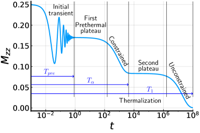
Figure 1: The plot shows the complete dynamics of the observable $M_{zz}$ as a function of $t$ in log-scale. The plot was generated by solving FRQME in Eq. (2) for $\omega_{1}=2\pi\times 5$ KHz, $|\omega_{d_{m}}|=2\pi\times 5$ KHz, $\omega_{\circ}=2\pi\times 10$ MHz, $\tau_{c}=1$ $\mu$s, $\omega_{\text{\tiny{SL}}}=2\pi\times 3\times 10^{-2}$ KHz, and $M_{zz}|_{t\rightarrow 0}=\frac{1}{4}$. The choice of parameters ensures that regular relaxation comes into play long after the other dissipators have completed their part. The dynamics clearly show the emergence of multiple prethermal states and the cascaded journey to the final steady state. $T_{pre}$ shows the timescale at which the initial transients die out and the first prethermal state emerges. This state further decays under a constrained thermalization process, and the second prethermal plateau emerges after $T_{\alpha}$. The regular relaxation with a longer timescale $T_{1}$ finally takes the system to a steady state.

First, we show the complete solution of Eq. 2 in terms of one of the observables defined in Eq. 3 for the initial condition, $\rho_{\scriptscriptstyle S}|_{t\rightarrow 0}=|11\rangle\langle 11|$ (i.e. $M_{zz}|_{t\rightarrow 0}=\frac{1}{4}$) in fig. 1. The figure caption contains the parameters used for generating the plot. We observe a cascaded journey of this observable from the initial value to the final steady state. We shall analyze the cascaded evolution by systematically including various interactions with decreasing strengths.

We note that Chakrabarti et al. has recently described the emergence of prethermal plateau Chakrabarti and Bhattacharyya (2022), and hence we provide a brief review here. One needs to consider the strongest Liouvillian ($\mathcal{L}_{sec}$) to understand the dynamics. Only the effect of the secular parts are considered here $\left(\mathcal{H}_{tot}^{sec}=\mathcal{H}_{\scriptscriptstyle\rm DR}^{sec}+\mathcal{H}_{\scriptscriptstyle\rm DD}^{sec}\right)$ . The explicit form of $\hat{\mathcal{L}}_{sec}$ is given below,

$$\mathcal{L}_{sec}\rho_{\scriptscriptstyle S}(t) = -i\left[\mathcal{H}_{tot}^{sec},\rho_{\scriptscriptstyle S}(t)\right]-\tau_{c}\left[\mathcal{H}_{tot}^{sec},\left[\mathcal{H}_{tot}^{sec},\rho_{\scriptscriptstyle S}(t)\right]\right]$$ (4)

Drive and dipolar interaction can appear in both first order and second order of the above Eq. (4). Cross relaxation occurs due to the cross terms of $\mathcal{H}_{\scriptscriptstyle\rm S}(t)$ and $\mathcal{H}_{\scriptscriptstyle\rm DD}$ in the second order.

The dynamical equation for the collective coherence ($M_{x}$) and corresponding coupled observables which are connected to the quasi-conserved quantities are written as,

$$\dot{M}_{x} = -\frac{9}{4}\omega_{d_{0}}^{2}\tau_{c}M_{x}+6\omega_{1}\omega_{d_{0}}\tau_{c}M_{zz}-6\omega_{1}\omega_{d_{0}}\tau_{c}M_{yy}-3\omega_{d_{0}}M_{yz}$$ (5)

$$\dot{M}_{zz} = \frac{3}{4}\omega_{1}\omega_{d_{0}}\tau_{c}M_{x}-2\omega_{1}^{2}\tau_{c}M_{zz}+2\omega_{1}^{2}\tau_{c}M_{yy}+\omega_{1}M_{yz}$$ (6)

$$\dot{M}_{yy} = -\frac{3}{4}\omega_{1}\omega_{d_{0}}\tau_{c}M_{x}+2\omega_{1}^{2}\tau_{c}M_{zz}-2\omega_{1}^{2}\tau_{c}M_{yy}-\omega_{1}M_{yz}$$ (7)

$$\dot{M}_{yz} = \frac{3}{4}\omega_{d_{0}}M_{x}-2\omega_{1}M_{zz}+2\omega_{1}M_{yy}-(4\omega_{1}^{2}+\frac{9}{4}\omega_{d_{0}}^{2}\tau_{c})M_{xy}$$ (8)

We note that the above equations show several constants of motion. For example, from the above, we infer, $M_{yy}+M_{zz}$, $3\omega_{d_{0}}M_{zz}+\omega_{1}M_{x}$ are constants. From the other equations (not shown), we also have $\dot{M}_{xx}=0$, and hence $M_{xx}$ is also a conserved quantity. However, as one includes other non-secular terms, the quantities may not be conserved. But being weaker than secular parts, the effect of non-secular terms becomes evident in the later part of the dynamics. As such, these quantities appear to be constant for a while and then undergo changes. Following Peng et al. we term these quantities as quasi-conserved Peng et al. (2021). Since the presence of the coherence $M_{x}$ as an arrested state was observed recently by Beatrez et al. Beatrez et al. (2021), we name the quasi-conserved quantity $3\omega_{d_{0}}M_{zz}+\omega_{1}M_{x}$ as the prethermal order. Similarly, we have another quasi-conserved quantity $M_{xx}+M_{yy}+M_{zz}$; this is the expectation value of $J^{2}\propto\vec{\sigma}^{1}.\vec{\sigma}^{2}$, and we name it the dipolar order. The quasi-conserved quantities can also be analyzed by using the eigen-spectrum of $\mathcal{L}_{sec}$. It has four zero-eigenvalues. One of the zero eigenvalues corresponds to the preservation of the trace. The three other zero eigenvalues correspond to the above three quasi-conserved quantities.

While solving the equation, the initial condition is chosen as $M_{zz}|_{t\rightarrow 0}=M_{\circ}$ and other observables as zero. The solution of $M_{zz}(t)$ from Eq. (4) is given by,

$$M_{zz}^{\text{\tiny{pre}}}(t) = \frac{M_{\circ}}{4}\left(1-\frac{2\omega_{1}^{2}}{\kappa_{1}^{2}}\left(1-\cos(\kappa_{1}t)e^{-t\kappa_{1}^{2}\tau_{c}}\right)\right)$$ (9)

where, $\kappa_{1}^{2}=4\omega_{1}^{2}+9\omega_{d_{0}}^{2}/4$. Therefore, $M_{zz}|_{t\rightarrow\infty}=\frac{M_{\circ}}{4}(1-2\omega_{1}^{2}/\kappa_{1}^{2})$ . The above solution shows that the initial transient phase oscillates with a frequency $\kappa_{1}$ and it reaches the prethermal steady state $(M_{zz}|_{t\rightarrow\infty})$ in a characteristic time-scale $T_{pre}=1/\left(\tau_{c}\kappa_{1}^{2}\right)$. In Fig. 1, $T_{pre}$ indicates the timescale of the system to reach the prethermal state from the initial transient phase.

Next, we include $\hat{\mathcal{L}}_{n}\hat{\rho_{\scriptscriptstyle S}}$ in the dynamics, whose form is given by,

$$\mathcal{L}_{n}\rho_{\scriptscriptstyle S}=-i[\mathcal{H}_{bs}+\mathcal{H}_{ds},\rho_{\scriptscriptstyle S}]+\mathcal{D}_{1}\rho_{\scriptscriptstyle S}+\mathcal{D}_{2}\rho_{\scriptscriptstyle S}$$ (10)

The shift terms are the Kramers-Kronig pairs of the second-order dissipative terms of the non-secular parts. They result in the re-normalization of the Zeeman frequency. $\mathcal{H}_{bs}$ is called the Bloch-Siegert shift, $\mathcal{H}_{bs}=2\omega_{1}^{2}\omega_{\circ}\tau_{c}\mathcal{Z}(2)I_{z}^{i}$, similarly $\mathcal{H}_{ds}$ represents the second-order dipolar shift; the expression is given by $\mathcal{H}_{ds}=(\omega_{d_{1}}^{2}\omega_{\circ}\tau_{c}\mathcal{Z}(1)+2\omega_{d_{2}}^{2}\omega_{\circ}\tau_{c}\mathcal{Z}(2))I_{z}^{i}$. Here $\mathcal{Z}(m)=\tau_{c}/\left(1+(m\omega_{\circ}\tau_{c})^{2}\right)$. These shift terms do not contribute to the decay rate and minimally affect the steady-state configuration, so we ignore them in the rest of the analysis. The explicit forms of the dissipative operators in Eq. (10) can be written as,

$$\mathcal{D}_{1}\rho_{\scriptscriptstyle S} = \sum\limits_{m=-2}^{2}|\omega_{d_{m}}|^{2}\mathcal{Z}(m)\left[2\mathcal{T}_{2}^{-m}\rho_{\scriptscriptstyle S}\mathcal{T}_{2}^{m}-\left\{\mathcal{T}_{2}^{m}\mathcal{T}_{2}^{-m},\rho_{\scriptscriptstyle S}\right\}\right]\quad[\forall m\neq 0]$$

$$\mathcal{D}_{2}\rho_{\scriptscriptstyle S} = \sum\limits_{i,j=1}^{2}\omega_{1}^{2}\mathcal{Z}(2)\left[2I_{\pm}^{i}\rho_{\scriptscriptstyle S}I_{\mp}^{j}-\left\{I_{\mp}^{j}I_{\pm}^{i},\rho_{\scriptscriptstyle S}\right\}\right]$$ (11)

We analyze the above Eq. (10) using the observables defined earlier in Eq. (3). The super-operator, $\hat{\mathcal{L}_{sec}}+\hat{\mathcal{L}_{n}}$ has two zero eigenvalues. In the presence of the non-secular terms, two of the earlier four quasi-conserved quantities will no longer be conserved. The prethermal state does not survive in this regime, as $3\omega_{d_{0}}\dot{M}_{zz}+\omega_{1}\dot{M}_{x}\neq 0$. Also, we have $\dot{M}_{xx}\neq 0$ and, $\dot{M}_{zz}+\dot{M}_{yy}\neq 0$. But the dipolar order still survives, ($\dot{M}_{xx}+\dot{M}_{yy}+\dot{M}_{zz}=0$). Therefore this regime shows a constrained thermalization, as the initial memory partly survives. The resulting equation of the observables are,

$$\dot{M}_{x} = -(2q_{1}+\frac{5}{2}p_{1}+p_{2})M_{x}+\text{terms in Eq. (\ref{eq-pre1})}$$

$$\dot{M}_{zz} = -(8q_{1}+2p_{1})M_{zz}+(4q_{1}+p_{1})(M_{xx}+M_{yy})+\text{terms in Eq. (\ref{eq-pre2})}$$

$$\dot{M}_{yy} = -(4q_{1}+p_{2}+p_{1})M_{yy}+p_{2}M_{xx}+(4q_{1}+p_{1})M_{zz}+\text{terms in Eq. (\ref{eq-pre3})}$$

$$\dot{M}_{xx} = -(4q_{1}+p_{2}+p_{1})M_{xx}+p_{2}M_{yy}+(4q_{1}+p_{1})M_{zz}$$ (12)

Here $q_{1}=\omega_{1}^{2}\mathcal{Z}(2)$ and $p_{m}=|\omega_{d_{m}}|^{2}\mathcal{Z}(m)$. In the limit of $\omega_{\circ}\tau_{c}>1$, the solution of transverse magnetization mode $M_{zz}(t)$ is written as,

$$M_{zz}(t) \approx \frac{M_{\circ}}{3}-e^{-t/T_{\alpha}}\left(\frac{M_{\circ}}{3}-M_{zz}^{\text{\tiny{pre}}}(t)\right)$$ (13)

$$\frac{1}{T_{\alpha}} = 3\left(p_{1}+4q_{1}\right)$$

Hence, the above solution of $M_{zz}(t)$ gives the notion of decay of prethermal order. $T_{\alpha}$ is the decay rate due to the non-secular part.

The dynamics of the other observables connected to prethermal order and dipolar order $\{M_{x},\,M_{xx},\,M_{yy},\,M_{zz}\}$ are also shown in Fig.2(a). The observables $\{M_{yy},\,M_{zz}\}$ get non-zero steady-state values in the prethermal time-regime, and $M_{xx}$ remains zero. Then at a later time, they begin to evolve. The constrained thermalization is shown in the time regime $T_{\alpha}$ of Fig.1. The aforementioned terms in Eq. (10) give an effective decay in the dynamics. The decay time is denoted as $T_{\alpha}$. The expression of the decay rate is given in Eq. (13). It is generally expressed as $1/T_{\alpha}\propto\frac{1/T_{pre}}{1+(\omega_{\circ}\tau_{c})^{2}}$. If one begins with $M_{x}|_{t\rightarrow 0}\neq 0$ and other observables are zero, then it replicates the spin-locking phenomena in nuclear magnetic resonance (NMR) and the recent experiment by Beatrez et al. Beatrez et al. (2021).

For a very weak system-bath interaction (long $T_{1}$ process), the timescale corresponding to the decay of quasi-equilibrium state is denoted as $T_{1\rho}$ in the spin-temperature theory of NMR Slichter (1996). In our case, $T_{\alpha}$ is equivalent to $T_{1\rho}$. The necessary condition for having a prethermal plateau is $T_{\alpha}\gg T_{pre}$. Therefore, to fulfill this condition, we must have $\omega_{\circ}\tau_{c}\gg 1$. In this limit, $1/T_{pre}\propto\tau_{c}$ and $1/T_{\alpha}\propto 1/\tau_{c}$.

It is known that, in the case of the dynamics of a dissipative system, the eigenvalues of $\mathcal{\hat{L}}$ must lie in the non-positive plane. The imaginary part of the eigenvalue comes from the unitary process due to the first-order terms and shift terms. On the other hand, the real part depicts the non-unitary dissipation Albert and Jiang (2014). The lifetime of the prethermal plateau is independent of the unitary process, so we neglect the imaginary part of the eigenvalue of $\mathcal{\hat{L}}$ for the rest of the analysis.

In this regime, $\mathcal{L}$ has two zero eigenvalues. Others are the decaying modes. The decay times are obtained by the inverse of the modulus of the eigenvalues. In Fig. 2(b), we have plotted the modulus of the eigenvalues as a function of the dimensionless quantity $\omega_{\circ}\tau_{c}$. It shows that for $\omega_{\circ}\tau_{c}>1$, two eigenvalues are much smaller than the others. When the remaining twelve modes decay, those two modes still remain alive, and the system has a prethermal plateau of a finite lifetime. Whereas, for $\omega_{\circ}\tau_{c}<1$, all the fourteen modes decay nearly at the same time. Hence, the plateau will not survive in this regime.

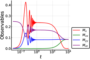
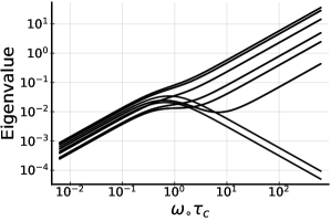
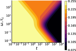
(a)     (b) (c) (d)    

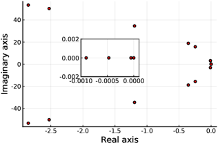
Figure 2: Subfigure (a) shows the plot of $\{M_{x},\,M_{xx},\,M_{yy},\,M_{zz}\}$ vs $t$. All the plots are done by numerically solving Eq. (4) and Eq. (10) simultaneously. The values of the parameters are given below, $\omega_{1}=2\pi\times 5$ KHz, $|\omega_{d_{m}}|=2\pi\times 5$ kHz, $\omega_{\circ}=2\pi\times 10$ MHz, $\tau_{c}=1$ $\mu$s. It shows that in the intermediate timescale, the prethermal order is preserved, but after a characteristic time, it decays. First two eigenvalues of total $\hat{\mathcal{L}}$ (excluding $\mathcal{H}_{\scriptscriptstyle\rm SL}$) are zero. Modulus of the other $14$ eigenvalues are plotted as a function of $\omega_{\circ}\tau_{c}$ in subfigure (b). For $\omega_{\circ}\tau_{c}>1$, The separate existence of the lowest two eigenstates from others is clearly visible. Whereas, for $\omega_{\circ}\tau_{c}\leqslant 1$, they merge. Subfigure (c) shows the filled contour of $M_{zz}(t)$ as a function of $\omega_{\circ}\tau_{c}$ and $t$. $\omega_{\circ}\tau_{c}\approx 1$ is the critical point of the dynamics. For $\omega_{\circ}\tau_{c}>1$, the orange (color online) triangular region shows the prethermal plateau. For $\omega_{\circ}\tau_{c}<1$, no such plateau forms. For (b) and (c), the effect of the imaginary part of the eigenvalues is neglected. Subfigure (d) shows the numerical plots for the distribution of the sixteen eigenvalues of $\hat{\mathcal{L}}_{sec}+\hat{\mathcal{L}}_{n}+\hat{\mathcal{L}}_{\text{\tiny{SL}}}$ in the real and imaginary axis. Here $P_{-}=1.6\times 10^{-5}$, $P_{+}=0.4\times 10^{-5}$ The lowest four eigenvalues are close to zero and are merged. The inset in the middle of the plot shows those four eigenvalues with an enlarged scale. The first two eigenvalues in the inset from the left are responsible for the prethermal plateau. The third one (from the left) shows the notion of constrained thermalization. The right one leads the system to the final steady state.

The solution of $M_{zz}(t)$ as a function of time and for the specific choice of $\omega_{\circ}\tau_{c}$ is shown in the contour plot (Fig. 2(c)). It depicts clearly a critical point at $\omega_{\circ}\tau_{c}=1$. For $\omega_{\circ}\tau_{c}>1$, there exist two distinct decay rates. The prethermal plateau is clearly visible in the regime. As we increase the value of $\omega_{\circ}\tau_{c}$, the length of the plateau increases as the differences between the eigenvalues grow. For, $\omega_{\circ}\tau_{c}<1$, the plateau ceases to exist. This criticality is reminiscent of the behavior of the relaxation rates due to spin-lattice relaxation as a function $\omega_{\circ}\tau_{c}$, as reported by Bloembergen and others Bloembergen et al. (1948, 1947). They found that for high motional narrowing, $\omega_{\circ}\tau_{c}<1$, and for the other regime (large macromolecules or solids) $\omega_{\circ}\tau_{c}>1$.

For the chosen parameters, the effect of $\mathcal{H}_{\scriptscriptstyle\rm SL}$ is prominent after the system reaches the unconstrained thermalization regime. We are not using any specific form of system-bath coupling; we introduce the relaxation rates in terms of known parametric form in the equation, as shown below. The form of $\hat{\mathcal{L}}_{\text{\tiny{SL}}}$ is given by,

$$\mathcal{L}_{\text{\tiny{SL}}}\rho_{\scriptscriptstyle S} = -i\left[\mathcal{H}_{\text{\tiny{lamb}}},\rho_{\scriptscriptstyle S}\right]+\mathcal{D}_{3}\rho_{\scriptscriptstyle S}$$ (14)

$\mathcal{H}_{\text{\tiny{lamb}}}$ is known as Lamb shift. It also has a minimal contribution to the steady state. The form is $D_{3}\rho_{\scriptscriptstyle S}$ is given by,

$$D_{3}\rho_{\scriptscriptstyle S} = \sum\limits_{i=1}^{2}P_{\mp}\left[2I_{\mp}^{i}\rho_{\scriptscriptstyle S}I_{\pm}^{i}-\{I_{\pm}^{i}I_{\mp}^{i},\rho_{\scriptscriptstyle S}\}\right],$$ (15)

where $P_{-},P_{+}$ is defined as the probability of the downward and upward transition due to $\mathcal{H}_{\scriptscriptstyle\rm SL}$ Heinz-Peter Breuer (2002). The form of $P_{-}$, $P_{+}$, and the dynamical equation in terms of the observables are shown in our earlier work Saha and Bhattacharyya (2022b). In the presence of only $\mathcal{H}_{\scriptscriptstyle\rm SL}$ (excluding $\mathcal{H}_{\scriptscriptstyle\rm S}(t)$, $\mathcal{H}_{\scriptscriptstyle\rm DD}$), the final density matrix is diagonal. For this case, the steady-state solution is given by, $M_{z}|_{t\rightarrow\infty}=\frac{P_{-}-P_{+}}{P_{-}+P_{+}}$, $M_{zz}|_{t\rightarrow\infty}=\left(M_{z}|_{t\rightarrow\infty}\right)^{2}/4$, and $T_{1}=1/(P_{+}+P_{-})$.

The total Liouvillian ( $\hat{\mathcal{L}}$) has a single zero eigenvalue, which means the steady state is unique and it has no initial memory. Under the evolution of $\mathcal{H}_{\scriptscriptstyle\rm SL}$, the dipolar order is broken, $\left[\dot{M}_{xx}+\dot{M}_{yy}+\dot{M}_{zz}\neq 0\right]$. Therefore the system reaches a final steady state under the evolution of full $\mathcal{L}$. The distribution of the eigenvalues is plotted in fig. 2(d). In the inset, the first three eigenvalues (from the left in the inset) decay at a longer time scale. Among them, the first two are responsible for the prethermal plateau, and the third one is for constrained thermalization, as only the dipolar mode survives after the prethermal state decays. The zero eigenvalue stands for the steady state; it appears when all fifteen eigenmodes decay.

The decay rate of the dipolar order is much slower than the prethermal order. This kind of quasi-conservation law was recently predicted by Peng et al. in kicked dipolar model Peng et al. (2021). The characteristic decay time is denoted as $T_{1}$ [$1/T_{1}\propto\frac{\omega_{sl}^{2}\tau_{c}}{1+(\omega_{\circ}\tau_{c})^{2}}$]. For $T_{\alpha}\gg T_{1}$, there exists another plateau in the system, which is shown in Fig. 1. For $\omega_{\circ}\tau_{c}<1$, [$T_{\alpha}\approx T_{pre}$], the initial transient phase skips the prethermal plateau and directly goes to the second plateau, whereas, for $T_{1}\gg T_{\alpha},T_{pre}$, the system directly arrives at the steady state, as there is no existence of prethermalization.

Table 1: comparison of different dynamical phases

Dynamical Phase	Liouvillian	Quasi-conserved quantity	Dark state
Prethermalization	$\hat{\mathcal{L}}_{sec}$	(a) $3\omega_{d_{0}}M_{zz}+\omega_{1}M_{x}$,	All eigenstates
		(b) $M_{xx}$, (c) $M_{yy}+M_{zz}$	corresponding to (a)
Constrained thermalization	$\hat{\mathcal{L}}_{sec}+\hat{\mathcal{L}}_{n}$	(a) $M_{xx}+M_{yy}+M_{zz}$	Only Singlet state
Unconstrained thermalization	$\hat{\mathcal{L}}_{sec}+\hat{\mathcal{L}}_{n}+\hat{\mathcal{L}}_{\text{\tiny{SL}}}$	None	None

The cascaded dynamics can be analyzed by the existence of the dark states in each regime. The non-equilibrium steady state ($\rho_{\infty}$) is defined as the null vector of the Liouvillian ($\mathcal{L}\rho_{\infty}=0$). If $\rho_{\infty}$ is a pure density matrix ($\rho_{\infty}=|\psi_{\infty}\rangle\langle\psi_{\infty}|$), then $|\psi_{\infty}\rangle$ is defined as dark state Buča and Prosen (2012). Here, in the prethermal regime, all the eigenstates of the observables corresponding to the prethermal order act as a dark state. When the prethermal plateau decays, three of the previous four states are no longer dark states. In the constrained thermalization regime, only the Bell singlet state ($\frac{1}{\sqrt{2}}(|10\rangle-|01\rangle)$) is acting as a dark state. Finally, when the system reaches unconstrained thermalization, there exists no dark state in the system. Table 1 shows the summary of the above description.

A long prethermal plateau is useful for designing sensitive magnetometers and quantum-sensors Beatrez et al. (2021). The necessary condition for this is $T_{pre}\ll T_{\alpha}\ll T_{1}$ or $\omega_{\circ}\tau_{c}\gg 1$. One can design a system to have a strong dipolar coupling and can apply a strong drive to achieve this condition at any given temperature. We show here the simple case of a dipolar-coupled two-spin system, whereas in the actual experiment, a dipolar network is considered. Our results show good agreement with the recent experiments by Beatrez et al. , and it can be extended to the dipolar network.

In summary, we present here the complete dynamical theory of periodically driven dissipative dipolar system using FRQME. We show that the journey to the equilibrium for such systems is a multi-stage process. The initial transient phase is governed by the first-order unitary processes. The second-order cross-relaxation process leads to the prethermal state. This prethermal state further decays due to the non-secular part of the drive and dipolar Hamiltonian. We calculate an effective decay rate that predicts the lifetime of such a state. We show that there exists a critical limit to the temporal correlation of the local environmental fluctuation. Beyond the limit, the prethermal plateau does not survive. We also observe that there exists another quasi-conserved quantity, even after the prethermal state vanishes. Finally, we discuss the effect of the system-bath coupling, which leads the system to the final steady state. The analysis in the above has been carried out using specific values of system parameters to demonstrate the possible existence of multiple prethermal plateaus. However, we note that for strong system-environment coupling, there may not be a well-defined thermal plateau as the timescales of various may overlap with each other. We envisage that this theoretical exposition of complete dynamics of a driven dissipative dipolar system will pave the way to a better understanding of the thermalization problem.

The authors thank Prasanta K. Panigrahi, Arpan Chatterjee, and Arnab Chakrabarti for their insightful comments and helpful suggestions. SS gratefully acknowledges University Grants Commission for a research fellowship (Student ID: MAY2018- 528071).

References

- Berges et al. (2004) J. Berges, S. Borsányi, and C. Wetterich, Physical Review Letters 93, 142002 (2004).
- Sen et al. (2004) S. Sen, T. R. K. Mohan, and J. M. M. Pfannes, Physica A: Statistical Mechanics and its Applications 342, 336 (2004).
- Deutsch (2018) J. M. Deutsch, Reports on Progress in Physics 81, 082001 (2018).
- Ueda (2020) M. Ueda, Nature Reviews Physics 2, 669 (2020).
- Deutsch (1991) J. M. Deutsch, Physical Review A 43, 2046 (1991).
- Srednicki (1994) M. Srednicki, Physical Review E 50, 888 (1994).
- Srednicki (1999) M. Srednicki, Journal of Physics A: Mathematical and General 32, 1163 (1999).
- Kuwahara et al. (2016) T. Kuwahara, T. Mori, and K. Saito, Annals of Physics 367, 96 (2016).
- Abanin et al. (2015) D. A. Abanin, W. De Roeck, and F. Huveneers, Physical Review Letters 115, 256803 (2015).
- Fleckenstein and Bukov (2021) C. Fleckenstein and M. Bukov, Physical Review B 103, L140302 (2021).
- Holthaus (2016) M. Holthaus, Journal of Physics B: Atomic, Molecular and Optical Physics 49, 013001 (2016).
- Weidinger and Knap (2017) S. A. Weidinger and M. Knap, Scientific Reports 7, 45382 (2017).
- Bukov et al. (2015a) M. Bukov, S. Gopalakrishnan, M. Knap, and E. Demler, Physical Review Letters 115, 205301 (2015a).
- Yin et al. (2021) C. Yin, P. Peng, X. Huang, C. Ramanathan, and P. Cappellaro, Physical Review B 103, 054305 (2021).
- Bukov et al. (2015b) M. Bukov, L. D’Alessio, and A. Polkovnikov, Advances in Physics 64, 139 (2015b).
- Rubio-Abadal et al. (2020) A. Rubio-Abadal, M. Ippoliti, S. Hollerith, D. Wei, J. Rui, S. Sondhi, V. Khemani, C. Gross, and I. Bloch, Physical Review X 10, 021044 (2020).
- Viebahn et al. (2021) K. Viebahn, J. Minguzzi, K. Sandholzer, A.-S. Walter, M. Sajnani, F. Görg, and T. Esslinger, Physical Review X 11, 011057 (2021).
- Beatrez et al. (2021) W. Beatrez, O. Janes, A. Akkiraju, A. Pillai, A. Oddo, P. Reshetikhin, E. Druga, M. McAllister, M. Elo, B. Gilbert, D. Suter, and A. Ajoy, Physical Review Letters 127, 170603 (2021).
- Peng et al. (2021) P. Peng, C. Yin, X. Huang, C. Ramanathan, and P. Cappellaro, Nature Physics 17, 444 (2021).
- Neyenhuis et al. (2017) B. Neyenhuis, J. Zhang, P. W. Hess, J. Smith, A. C. Lee, P. Richerme, Z.-X. Gong, A. V. Gorshkov, and C. Monroe, Science Advances 3, e1700672 (2017).
- Chakrabarti and Bhattacharyya (2018) A. Chakrabarti and R. Bhattacharyya, Phys. Rev. A 97, 063837 (2018).
- Chatterjee and Bhattacharyya (2020) A. Chatterjee and R. Bhattacharyya, Phys. Rev. A 102, 043111 (2020).
- Chanda and Bhattacharyya (2021) N. Chanda and R. Bhattacharyya, Phys. Rev. A 104, 022436 (2021).
- Chanda and Bhattacharyya (2020) N. Chanda and R. Bhattacharyya, Phys. Rev. A 101, 042326 (2020).
- Saha and Bhattacharyya (2022a) S. Saha and R. Bhattacharyya, Journal of Magnetic Resonance Open 10-11, 100046 (2022a).
- Saha and Bhattacharyya (2022b) S. Saha and R. Bhattacharyya, Journal of Physics B: Atomic, Molecular and Optical Physics 55, 235501 (2022b).
- Chakrabarti and Bhattacharyya (2022) A. Chakrabarti and R. Bhattacharyya, arXiv preprint arXiv:1911.07607 (2022).
- Claude Cohen-Tannoudji (1998) G. G. Claude Cohen-Tannoudji, Jacques Dupont-Roc, Atom-photon interactions: basic processes and applications, wiley ed. (Wiley-VCH, 1998).
- Slichter (1996) C. P. Slichter, Principles of Magnetic Resonance (3rd Enlarged and Updated Edition) (Springer, 1996).
- Albert and Jiang (2014) V. V. Albert and L. Jiang, Phys. Rev. A 89, 022118 (2014).
- Bloembergen et al. (1948) N. Bloembergen, E. M. Purcell, and R. V. Pound, Physical Review 73, 679 (1948).
- Bloembergen et al. (1947) N. Bloembergen, E. M. Purcell, and R. V. Pound, Nature 160, 475 (1947).
- Heinz-Peter Breuer (2002) F. P. Heinz-Peter Breuer, The Theory of Open Quantum Systems (Oxford University Press, 2002).
- Buča and Prosen (2012) B. Buča and T. Prosen, New Journal of Physics 14, 073007 (2012).