A Bayesian Approach to Reconstructing Interdependent Infrastructure Networks from Cascading Failures

Abstract

Analyzing the behavior of complex interdependent networks requires complete information about the network topology and the interdependent links across networks. For many applications such as critical infrastructure systems, understanding network interdependencies is crucial to anticipate cascading failures and plan for disruptions. However, data on the topology of individual networks are often publicly unavailable due to privacy and security concerns. Additionally, interdependent links are often only revealed in the aftermath of a disruption as a result of cascading failures. We propose a scalable nonparametric Bayesian approach to reconstruct the topology of interdependent infrastructure networks from observations of cascading failures. Metropolis-Hastings algorithm coupled with the infrastructure-dependent proposal are employed to increase the efficiency of sampling possible graphs. Results of reconstructing a synthetic system of interdependent infrastructure networks demonstrate that the proposed approach outperforms existing methods in both accuracy and computational time. We further apply this approach to reconstruct the topology of one synthetic and two real-world systems of interdependent infrastructure networks, including gas-power-water networks in Shelby County, TN, USA, and an interdependent system of power-water networks in Italy, to demonstrate the general applicability of the approach.

1 Introduction

Networks offer a powerful tool for describing and analyzing various systems with complex interactions, such as ecological, biological, technological, and social systems [1, 2, 3]. Examples in infrastructure systems include modeling water distribution systems as a network wherein facilities like pumping stations and storage tanks are modeled as nodes and water pipes as links. Other examples include modeling interdependent infrastructures systems (e.g., coupled power and water systems) as multi-layer networks to analyze their vulnerability and resilience to disruptive events [4]. Ideally, performing such network-level assessments requires data from real infrastructure networks with complete information on the network topology, flow, and interdependencies. However, data on the topology of real-world infrastructure networks are often not available either due to privacy and security concerns or decentralized operations of different infrastructure sectors [5]. As a result, infrastructure network performance has been evaluated using model-driven techniques that rely on assumptions of the existence and importance of interdependencies. More recent research advances have focused on generating synthetic infrastructure data to overcome real network data challenges [6, 7, 8]. To achieve a more accurate representation of network interdependencies, this study proposes a data-driven approach to infer the structure of interdependent critical infrastructure (ICI) networks based on observations of cascading failures and other data sources.

Network reconstruction from observations of the dynamics on the target network is a fundamental but challenging inverse problem [9, 10]. This problem has garnered significant attention from researchers across several domains with research advances made to (i) capture network structure using partial information [11, 12, 13], and (ii) anticipate dynamic changes [14, 15, 16]. While applications such as social, biological, and ecological networks have obvious dynamic patterns, the structure of critical infrastructure networks has been assumed to be static and deterministic unless the structure is subject to disruptions. Some studies have applied network reconstruction to an individual infrastructure, such as road networks [17], but a generic approach for learning the topology of ICIs is still lacking.

1.1 Background and related work

Network reconstruction aims to infer the network topology from direct or indirect data that are inherently connected to the underlying network such as observations of dynamic processes on the network [18, 3, 9]. Examples of such dynamic processes include the diffusion of news among social media [19], the propagation of cascading failures in infrastructures [20], and the spreading of influence among political parties [21]. Although a single sequence of cascading failures may not provide sufficient information on the underlying network, combining many sequences of cascading failures can enable robust network reconstruction to obtain valuable insight into the functionality of the underlying network [22].

Data-driven network reconstruction approaches are divided into three categories: (i) graph embedding-based approach [23, 24, 25], (ii) optimization-based approach, and (iii) the Bayesian approach [26, 27, 9, 28]. Graph embedding-based approaches, including different types of graph neural networks [29, 30] that first require graph embedding, aim to map nodes into a low-dimensional vector space wherein the quantitative relationships among nodes reflect the topology of the original network [23, 24, 25]. The low-dimensional representation of the original networks is then used for link prediction. However, graph embedding-based approaches are not suitable for reconstructing infrastructure networks because graph embedding requires a relatively high amount of topological information about the target network, which is hard to obtain for real infrastructure systems. optimization-based approaches mainly include matrix factorization [31], compressed sensing [32, 33], and so forth. Similar to graph embedding-based approaches, Optimization-based approaches also assume that a subset of the target network is observed, therefore we resort to other approaches to tackle the problem of infrastructure networks reconstruction.

The Bayesian approach has been commonly used to uncover the complete network structure from partial observations [27] primarily due to their ability to allow for uncertainty measurement of estimated network topology, which is important because in many cases only sparse observations of failure cascades are available [9, 10]. Bayesian approaches for network reconstruction are either parametric or nonparametric. In parametric approaches, such as maximum likelihood estimation [34] or expectation maximization [35], the topology of the target network is usually assumed to be generated by a predefined statistical graph model. Then a fixed set of parameters of the parametric model are fitted such that the model is most likely to produce the data about the underlying network. Parametric models require that the network type is known, but many real-world systems are comprised of a diverse set of interconnected networks that do not fall into a well-defined network type.

In contrast, nonparametric approaches do not assume a particular model form and use a large number of samples of possible topologies to identify the most probable network. Topologies that are compatible with the observed dynamic process will have a higher posterior probability. Several models have been developed along this line. Peixoto [27] integrates a Bayesian approach with epidemic spreading models and the Ising model to learn the network structure and community labels simultaneously from measurements of network dynamics. Gray et al. [9] propose a similar Bayesian approach to infer the network structure that employs the independent cascade model of information diffusion for dynamical processes on networks, which is analogous to the susceptible-infected (SI) model for epidemic spreading. These models demonstrate the power of nonparametric Bayesian approach in reconstructing networks like social networks and information networks, but they are not specifically designed for infrastructure networks.

1.2 Contributions

In this paper, we develop a nonparametric Bayesian approach to infer the discrete posterior distribution of the topology of the target infrastructure networks from observations of cascading failures. The inference is performed using the Markov Chain Monte Carlo (MCMC) algorithm with infrastructure-dependent proposals. Our contributions are twofold:

1. We devise an infrastructure-dependent proposal in applying the MCMC algorithm for reconstructing different types of infrastructure networks with considerations to their unique topological constraints. Taking advantage of the block structure of ICI networks, we leverage the hierarchical stochastic block model (HSBM) to compute the prior probability of the potential graphs. The topological constraints guarantee that the topology of the proposed network matches that of the corresponding real infrastructure and significantly reduces the sampling space of network topology. The convergence of the graph MCMC algorithm is proved analytically and demonstrated numerically.

2. We design three computational optimization techniques to improve the efficiency of the graph MCMC algorithm in reconstructing large-scale networks where the number of possible network topologies grows exponentially over the number of nodes. The performances of these three techniques are demonstrated through experiments on reconstructing synthetic ICI networks.

The rest of this paper is organized as follows: Section 2 introduces the general Bayesian model for reconstructing the network topology based on cascading failures data. The graph MCMC algorithm with the infrastructure-dependent proposal to infer the Bayesian model is described in Section 3. In Section 4, we present three computational optimization techniques to improve the computational efficiency of the proposed network reconstruction approach. Numerical experiments for validating the proposed approach are shown in Section 5, followed by concluding remarks in Section 6.

2 Bayesian approach for network reconstruction

Network reconstruction using Bayesian approaches can be defined as follows.

Definition 1

(Network reconstruction). Given a set of time series data $\bm{C}$ about the binary state of nodes that are generated from a cascading failure process on a network with unknown adjacency matrix $\bm{A}$, the network structure is inferred by finding the adjacency matrix $\bm{A}$ with the highest conditional probability $P(\bm{A}|\bm{C})$. The set of cascading failure data $\bm{C}$ contains independent cascading failure scenarios (sequence) $\bm{c}^{i},i\in\{1,2,...C\}$ starting from time 1 where $\bm{c}^{i}_{t,j}=1$ indicates node $j$ fails at time $t$ in the $i$-th cascading failure scenario. The failure of node $j$ occurs when at least one of its adjacent nodes fails and this failure successfully propagates along links to the node $j$.

In the Bayesian approach for network reconstruction, we need to estimate the probability distribution density (PDF) of the network topology given the observations, i.e., a set of initial node failure scenarios and the following cascading failure sequences. Specifically, conditioned on the time series observations on node failures $\bm{C}$, we estimate the posterior distribution $P(\bm{A}|\bm{C})$ for the adjacency matrix $\bm{A}$ of the underlying network via Bayes’ rule [27, 9]:

$$P(\bm{A}|\bm{C})=\frac{P(\bm{C}|\bm{A})P(\bm{A})}{P(\bm{C})}\propto P(\bm{C}|\bm{A})P(\bm{A}),$$ (1)

where $P(\bm{C}|\bm{A})$ is the likelihood that the cascading failures $\bm{C}$ occur in a network with topology $\bm{A}$, $P(\bm{A})$ encodes the prior information on the network topology, and $P(\bm{C})$ is the normalization constant which represents the total evidence for the cascading failure data $\bm{C}$ [27]. Details on calculating the graph prior $P(\bm{A})$ and the likelihood $P(\bm{C}|\bm{A})$ are presented in Sections 2.1 and 2.2, respectively.

2.1 Hierarchical stochastic block model

This section introduces how to generate the prior probability of network topology using HSBM. Calculating the prior probability of the topology $P(\bm{A})$ requires realistic possible samples of the target network to be reconstructed. Different types of networks having different prior probabilities $P(\bm{A})$ can be generated by different graph models. The graph model we adopt here should represent the realistic behaviors of the target network. Generative graph models for real networks, such as the classical random network, scale-free network, and the small world network, are not applicable to real-world ICIs because nodes in infrastructure networks are grouped by blocks and hierarchy [36]. As such, a suitable model for characterizing ICI networks is the HSBM.

The HSBM is built on the stochastic block model which divides different nodes into different blocks using the membership of nodes. The HSBM then adds hierarchical structures in each block based on levels of node functionality in each block. As such, the probability of an edge between two nodes depends on the blocks to which the nodes belong and the hierarchical levels at which the nodes are positioned. Considering a multilayer network with a set of blocks $\mathcal{M}=\{M_{1},M_{2},...,M_{|\mathcal{M}|}\}$ and the number of nodes in each block is $n_{M},M\in\mathcal{M}$, each single block $M\in\mathcal{M}$ has a hierarchical structure $\mathcal{L}=\{L_{1},L_{2},...,L_{|\mathcal{L}|}\}$ where $n_{M}$ nodes are further divided into $|\mathcal{L}|$ levels. Considering the set of nodes and edges in the multilayer network as $\mathcal{V}^{\mathcal{M}}=\bigcup\limits_{M\in\mathcal{M}}{\mathcal{V}^{M}},\mathcal{E}^{\mathcal{M}}=\bigcup\limits_{M\in\mathcal{M}}{\mathcal{E}^{M}}$ and denoting the block and the level labels of the node $i$ as $m_{i}\in\mathcal{M}$ and $l_{i}\in\mathcal{L}$, then the probability of an edge $(i,j)$ is an independent Bernoulli random variable $p_{ij}$ conditioned on the block and the level labels $b_{i},b_{j},l_{i},l_{j}$ of nodes $i,j$. Therefore, the prior probability $P(\bm{A})$ conditioned on the block and layer assignment, $\mathcal{M}$ and $\mathcal{L}$, is calculated as

$$P(\bm{A}|\mathcal{M},\mathcal{L})=\prod\limits_{\forall i,j\in\mathcal{V}^{\mathcal{M}},i\neq j}{p_{ij}^{\bm{A}_{ij}}(1-p_{ij})^{1-\bm{A}_{ij}}},$$ (2)

$$p_{ij}=g(b_{i},b_{j},l_{i},l_{j}),$$ (3)

where $g$ is a HSBM function that calculates the edge probability based on the block and the layer assignments of nodes. Conditioning the graph prior probability $P(\bm{A})$ on the HSBM model, we introduce prior knowledge on network topology $P(\bm{A}|\mathcal{M},\mathcal{L})$ from the function $g$. In ICIs, $\mathcal{M}$ corresponds to individual infrastructure sectors (e.g., power grid, gas distribution network) and $\mathcal{L}$ represents different types of facilities with different functionalities (e.g., power supply and distribution nodes).

2.2 Cascading failure model

After employing the HSBM to model the prior information on the network topology, we further utilize the cascading failure model to compute the likelihood used in Eq. (1) in this section. Denoting the adjacency matrix of the network to be reconstructed as $\bm{A}^{*}$, the prior knowledge on the network topology is updated with the likelihood $P(\bm{C}|\bm{A})$ towards the target topology $\bm{A}^{*}$ that determines the diffusion of the cascading failure encoded in $\bm{C}$. Disasters cause initial failures of infrastructure components, which then trigger flow redistribution of resources and energy within and across the infrastructure networks [37, 38]. The flow redistribution will then overload and damage additional components, leading to cascading failures until the system reaches a new stable state without newly failed components. We leverage the SI model to simulate the cascading failure occurring on infrastructure networks wherein the failure of facilities is modelled by the ‘infection’ of nodes and the flow redistribution is modelled by the probabilistic propagation of the infection in the network.

Considering a failure propagation from time step $t$ to $t+1$ on node $j$ shown in Fig. 1 and further assuming that the probability of failure propagating from node $i$ to $j$ is $q_{ij}$, the failure probability of node $j$ is calculated as

$$P(\bm{c}^{i}_{t+1,j} =1|\bm{c}^{i}_{t,j}=0,\bm{c}^{i}_{t,1}=1...,\bm{c}^{i}_{t,v}=0)$$

$$=1-(1-q_{1j})(1-q_{2j})\cdots(1-q_{{v-1}j}).$$ (4)

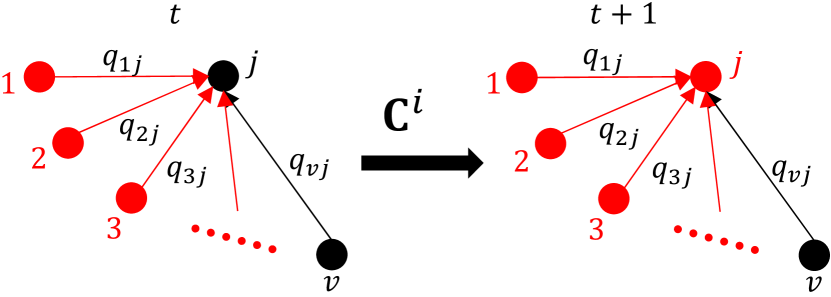
Figure 1: Failure propagation from time $t$ to $t+1$ for node $j$, red represents failed nodes while black represents nodes that are still functional.

Due to the independence between the two cascading failure scenarios $\bm{c}^{i}$ and $\bm{c}^{j}\;(i\neq j,i,j\in\{1,...,C\}$, the likelihood of the cascading failure data $\bm{C}$ encodes the failure propagation across all cascading failure scenarios $i\in\{1,...,C\}$, over all time steps for the entire disruption duration $\{1,...,T(\bm{c}^{i})\}$, and among all nodes in the multilayer network $j\in\mathcal{V}^{\mathcal{M}}$. This likelihood is given by

$$P(\bm{C}|\bm{A}^{M})=\prod\limits^{C}_{i=1}{\prod\limits_{t=1}^{T(\bm{c}^{i})}{\prod\limits_{j=1}^{|\mathcal{V}^{\mathcal{M}}|}{P(\bm{c}^{i}_{t+1,j}|\bm{c}^{i}_{t})}}},$$ (5)

where $T(\bm{c}^{i})$ is the number of time steps that the cascading failure scenario $\bm{c}^{i}$ lasts and $P(\bm{c}^{i}_{t+1,j}|\bm{c}^{i}_{t})$ is the probability of the status of operation of node $j$ at time step $t+1$, which is calculated by incorporating operable node status into Eq. (2.2):

$$P\left(\bm{c}^{i}_{t+1,j}|\bm{c}^{i}_{t}\right)$$

$$={\left[{1-{\prod_{k\in\{{{\cal V}^{\cal M}}\backslash j\}}}\left[{1-{q_{kj}}{\bm{A}_{kj}}\bm{c}_{t,k}^{i}(1-{\rm{}}\bm{c}_{t-1,k}^{i})}\right]}\right]^{\bm{c}_{t+1,j}^{i}(1-\bm{c}_{t,j}^{i})}}$$

$$\;\cdot{\left[{{\prod_{k\in\{{{\cal V}^{\cal M}}\backslash j\}}}\left[{1-{q_{kj}}{\bm{A}_{kj}}\bm{c}_{t,k}^{i}(1-{\rm{}}\bm{c}_{t-1,k}^{i})}\right]}\right]^{(1-\bm{c}_{t+1,j}^{i})(1-\bm{c}_{t,j}^{i})}},$$ (6)

where the first term on the right-hand side represents the probability of failure propagating to node $j$ while the second term represents the failure probability of its complementary event, i.e. failure not propagating to node $j$. The complementary property is guaranteed by the fact that only one of the two binary terms $\bm{c}^{i}_{t+1,j}(1-\bm{c}^{i}_{t,j})$ and $(1-\bm{c}^{i}_{t+1,j})(1-\bm{c}^{i}_{t,j})$ can be 1. The term $\bm{c}^{i}_{t,k}(1-\bm{c}^{i}_{t-1,k})$ ensures that the failure propagation is Markovian, i.e. the failure of nodes at the current time step is only impacted by nodes that failed at the last time step, which matches the failure process of infrastructure networks, such as the progressive collapse of structures and gradual outages of the power stations [39]. For non-Markovian failure propagation wherein nodes that fail several time steps ago can still affect nodes at the current time step, such as information diffusion and epidemic spreading in social networks, one can simply remove the term $\bm{c}^{i}_{t-1,k}$ to incorporate these cases into the cascading failure model.

3 Graph MCMC for network reconstruction

By generating possible network topologies with the graph prior model from Section 2.1 and incorporating the cascading failure model in Section 2.2, Eq. (1) becomes

$$P(\bm{A}|\bm{C},\mathcal{M},\mathcal{L})\propto P(\bm{C}|\bm{A},\mathcal{M},\mathcal{L})P(\bm{A}|\mathcal{M},\mathcal{L})P(\mathcal{M},\mathcal{L}),$$ (7)

where $P(\bm{C}|\bm{A},\mathcal{M},\mathcal{L})$ is the likelihood and $P(\bm{A}|\mathcal{M},\mathcal{L})\cdot P(\mathcal{M},\mathcal{L})$ is the prior probability of the network topology. Since the cascading failure scenarios, $\bm{C}$, are not related to blocks and layers assignments, $\mathcal{M}$ and $\mathcal{L}$, in calculating the prior probability of proposed networks by the HSBM, the likelihood is

$$P(\bm{C}|\bm{A},\mathcal{M},\mathcal{L})=P(\bm{C}|\bm{A}).$$ (8)

Given that $P(\mathcal{M},\mathcal{L})$ does not contain $\bm{A}$ and using Eq. (8), Eq. (7) is simplified as follows

$$P(\bm{A}|\bm{C},\mathcal{M},\mathcal{L})\propto P(\bm{C}|\bm{A})P(\bm{A}|\mathcal{M},\mathcal{L}).$$ (9)

3.1 Metropolis-Hastings algorithm

Since Eq. (9) usually does not have a closed-form solution, simulation techniques are typically leveraged to generate samples of the posterior distributions of possible network topologies. MCMC methods such as Metropolis-Hastings (M-H) algorithm and Gibbs sampling are commonly used to perform the Bayesian inference through sampling [40, 41]. In this study, M-H algorithm is employed to implement the proposed Bayesian approach since the Gibbs sampling algorithm requires an analytical solution to the conditional distributions of each parameter in the model. At each step in the M-H algorithm, a new multilayer network $\mathcal{M}^{\prime}$ with topology $\bm{A}^{\prime}$ is proposed based on the current network $\mathcal{M}$ with topology $\bm{A}$ using the proposal distribution $Q(\bm{A}^{\prime}|\bm{A})$. The M-H algorithm accepts the new proposal probabilistically with the ratio $\gamma$, which is given by

$$\gamma=\min(1,\frac{P(\bm{C}|\bm{A}^{\prime})P(\bm{A}^{\prime}|\mathcal{M},\mathcal{L})}{P(\bm{C}|\bm{A})P(\bm{A}|\mathcal{M},\mathcal{L})}\frac{Q(\bm{A}|\bm{A}^{\prime})}{Q(\bm{A}^{\prime}|\bm{A})}).$$ (10)

The performance of the algorithm depends on the choice of the proposal distribution $Q(\bm{A}^{\prime}|\bm{A})$. The random-walk graph proposal is commonly used in the M-H algorithm, where a random pair of nodes is chosen either by creating or removing the existing edges between them. However, this approach can generate invalid or unrealistic proposals of network topology. For example, in generating proposals of possible underlying topologies of interdependent water and power networks, a likely edge is from pumping stations to storage tanks, representing water extraction from nearby rivers at pumping stations and its transportation to storage tanks to be stored for future use. However, random graph proposals may add edges going from storage tanks to pumping stations which is not realistic. As such, we devise an infrastructure-dependent proposal method that imposes additional constraints on the topology of the proposed networks.

3.2 Infrastructure-dependent proposal

Infrastructure-dependent proposal ensures that only networks with a topology conforming to ICIs are considered. This is achieved by first analyzing the basic topology of ICIs, from which we abstract the topological constraints for designing the infrastructure-dependent proposal. We consider that each individual network in ICIs has a hierarchical structure with three levels corresponding to supply, transmission, and demand facilities. Given a set of infrastructure networks, $\mathcal{M}$, where supply, transmission and demand nodes are denoted as $\text{s},\text{t},\text{d}$, and a set of interdependent links, $\mathcal{I}$, across the networks, we can express the topological constraints as follows:

1. $\forall M\in\mathcal{M},\forall i\in\mathcal{V}_{\text{s}}^{M},\exists j\in\mathcal{V}_{\text{d}}^{M},i\mathop{\rightarrow}\limits^{\text{path}}j$.

2. $\forall M\in\mathcal{M},\forall i\in\mathcal{V}_{\text{d}}^{M},\exists j\in\mathcal{V}_{\text{s}}^{M},j\mathop{\rightarrow}\limits^{\text{path}}i$.

3. $\forall M\in\mathcal{M},\forall i\in\mathcal{V}_{\text{s}}^{M},\exists j\in\mathcal{V}_{\text{t}}^{M},i\mathop{\rightarrow}\limits^{\text{path}}j$.

4. $\forall M\in\mathcal{M},\forall i\in\mathcal{V}_{\text{t}}^{M},\exists j\in\mathcal{V}_{\text{s}}^{M},j\mathop{\rightarrow}\limits^{\text{path}}i$.

5. $\forall I\in\mathcal{I},\forall i\in\mathcal{V}_{\text{t}}^{I},\exists j\in\mathcal{V}_{\text{d}}^{I},i\mathop{\rightarrow}\limits^{path}j$.

6. $\forall I\in\mathcal{I},\forall i\in\mathcal{V}_{\text{d}}^{I},\exists j\in\mathcal{V}_{\text{t}}^{I},j\mathop{\rightarrow}\limits^{path}i$.

7. $\forall M\in\mathcal{M},\forall(i,j)\in\mathcal{E}^{M},i\in\mathcal{V}_{1},j\in\mathcal{V}_{2},\{\mathcal{V}_{1},\mathcal{V}_{2}\}\in\{\{\mathcal{V}^{M}_{\text{s}},\mathcal{V}^{M}_{\text{t}}\},\{\mathcal{V}^{M}_{\text{t}},\mathcal{V}^{M}_{\text{d}}\},\{\mathcal{V}^{M}_{\text{s}},\mathcal{V}^{M}_{\text{d}}\}\}$.

8. $\forall I\in\mathcal{I},\forall(i,j)\in\mathcal{E}^{I},i\in\mathcal{V}^{I}_{s},j\in\mathcal{V}^{I}_{d}$.

9. $\forall M\in\mathcal{M},\forall I\in\mathcal{I},\text{no cycles}$ in $M,I$.

Typically, resources are generated or extracted at supply nodes and transported via transmission nodes to demand nodes where resources are further distributed to local residents. Therefore, in every infrastructure network, $M\in\mathcal{M}$, every supply node $i\in\mathcal{V}^{M}_{\text{s}}$ is connected by a path to at least one demand node $j\in\mathcal{V}^{M}_{\text{d}}$ and vice versa, corresponding to constraints 1-2. Every transmission node $i\in\mathcal{V}^{M}_{\text{t}}$ is connected by a path from at least one supply node $j\in\mathcal{V}^{M}_{\text{s}}$ and to at least one demand node $k\in\mathcal{V}^{M}_{\text{d}}$, corresponding to the constraints 3-4. Similarly, for every interdependent link $I\in\mathcal{I}$, we have the same constraints for connectivity from the supply nodes to demand nodes, according to constraints 5-6. The resources move from supply nodes (at the high level) to demand nodes (at the low level) with no resources flowing back, which results in only forward edges from high level nodes to low level nodes according to constraints 7-8, which automatically leads to no cycles in each individual network as shown by constraint 9.

The M-H algorithm with infrastructure-dependent proposal and considerations of the nine constraints is outlined in Alg. 1. First a basic adjacency matrix $\bm{A}^{0}$ is generated following steps 1-5 to initiate the M-H algorithm. While we construct $\bm{A}^{0}$ by connecting failed nodes in sequential time steps, any method that generates graphs with $P(\bm{C}|\bm{A})>0$ could be used. In step 10, we randomly select a pair of nodes $(i,j)$ from the subset of the feasible set $\mathcal{S}=\{\{\mathcal{V}^{M}_{\text{s}},\mathcal{V}^{M}_{\text{t}}\},\{\mathcal{V}^{M}_{\text{s}},\mathcal{V}^{M}_{\text{d}}\},\{\mathcal{V}^{M}_{\text{t}},\mathcal{V}^{M}_{\text{d}}\},\{\mathcal{V}^{I}_{\text{s}},\mathcal{V}^{I}_{\text{d}}\}\},\forall M\in\mathcal{M},\forall I\in\mathcal{I}\}$, which guarantees that constraints (7)-(9) are satisfied. Then we add or remove the edge between that pair of nodes $(i,j)$ and generate a new candidate network following steps 11-15. The candidate network is accepted as a sample of the posterior distribution of $\mathcal{A}$, if the addition or removal of this edge does not violate constraints (1)-(6). Otherwise, we reject this candidate, propose another pair of nodes, and check the feasibility of the proposed topology, as shown in steps 16-22. Note that the block and layer assignments required in calculating the acceptance ratio, Eq. (10), are already given since blocks correspond to infrastructure networks $\mathcal{M},\mathcal{I}$ and layers correspond to facility types as defined in Section 2.1.

The advantage of this infrastructure-dependent proposal over the original one lies in the improvement in the sampling efficiency. By imposing additional topological constraints, invalid topology proposals are eliminated, thereby increasing the accuracy of sampling. Moreover, such elimination of invalid topology proposals reduces the space of the candidate topology (Appendix B), which significantly decreases the mixing time of the M-H algorithm. We also show that the Markov chain constructed using the infrastructure-dependent proposal converges (Appendix A).

  Algorithm 1: M-H algorithm with infrastructure-dependent proposal

 

1:The set of networks to be reconstructed $\mathcal{M},\mathcal{I}$ with known types of facilities in sets $\mathcal{V}^{M}_{\text{s}},\mathcal{V}^{M}_{\text{t}},\mathcal{V}^{M}_{\text{d}}$, the cascading failure data $\bm{C}$, the maximum number of iterations $Iter_{max}$, the feasible set $\mathcal{S}$ from which the pair of nodes for which an edge is added or removed is randomly picked

2:The posterior distribution of the adjacency matrix $\mathcal{A}$ of the target networks

3:for cascading failure scenario $i\in\{1,...,C\}$ do

4:     for $t\in\{1,...,T(\bm{c}^{i})-1\}$ do

5:         Add a link between every node failing at $t$ and

6:          every node failing at $t+1$

7:     end for

8:end for$\triangleright$ Initialize the adjacency matrix $\bm{A}^{0}$

9:$\text{Iter}\leftarrow 0$

10:while $\text{Iter}<=Iter_{max}$ do$\triangleright$ Start M-H sampling

11:     $\bm{A}\leftarrow\bm{A}^{\text{Iter}}$

12:     Randomly pick a pair of nodes $(i,j)$, $i\in\mathcal{V}_{1}$,

13:      $j\in$ $\mathcal{V}_{2}$ and the set $\{\mathcal{V}_{1},\mathcal{V}_{2}\}\in\mathcal{S}$

14:$\triangleright$ Impose constraints (7)-(9)

15:     if $\bm{A}_{ij}=0$ then

16:         $\bm{A}_{ij}\leftarrow 1$

17:     else

18:         $\bm{A}_{ij}\leftarrow 0$

19:     end if$\triangleright$ Add or remove the link

20:     if $\bm{A}$ causes no violation of constraints (1)-(6) then

21:         Calculate the acceptance ratio $\gamma$ by Eq. (10)

22:         if $\gamma\geq p\sim U(0,1)$ then

23:              Accept $\bm{A}$ as a sample of the posterior

24:              distribution of $\mathcal{A}$

25:              $\text{Iter}\leftarrow\text{Iter}+1$

26:         end if

27:     end if

28:end while

29:return $\mathcal{A}$

 

4 Computational techniques for improving the sampling efficiency

Although the infrastructure-dependent proposal significantly reduces the space of the candidate network topology and thus improves the sampling efficiency, the computational expense can still be very high due to the computation of proposing and updating the topology of the network at each iteration. At each iteration, steps 8-23 in Alg. 1 takes $\mathcal{O}(1)$ operations to randomly choose node pairs from the feasible set and add or remove associated links. Evaluating the likelihood $P(\bm{C}|\bm{A})$ in calculating the acceptance ratio $\gamma$ takes $\mathcal{O}(\sum_{i=1}^{C}{T(\bm{c}^{i})|\mathcal{V}^{\mathcal{M}}|^{2}})$ time to double loop over all nodes in $\mathcal{V}^{\mathcal{M}}$ at time step $t$ to compute the failure probability of every node at $t+1$ and iterate over all time steps in $\{1,...,T(\bm{c}^{i})-1\}$ through all cascading scenarios $\bm{c}^{i},i\in\{1,...,C\}$. Validating whether the generated network $\bm{A}$ violates constraints (1)-(6) requires $\mathcal{O}(|\mathcal{V}^{\mathcal{M}}|(|\mathcal{V}^{\mathcal{M}}|+|\mathcal{E}^{\mathcal{M}}|)+|\mathcal{V}^{\mathcal{I}}|(|\mathcal{V}^{\mathcal{I}}|+|\mathcal{E}^{\mathcal{I}}|))$ as we check the existence of paths by tree-search algorithms such as Depth First Search (DFS) or Breadth First Search (BFS) on every node in every network. So the total time of each iteration in Alg. 1 takes ${\cal O}(\underbrace{\sum\limits_{i=1}^{C}{T({\bm{c}^{i}})|{{\cal V}^{\cal M}}}{|^{2}}}_{{\text{Likelihood calculation}}}+\underbrace{|{{\cal V}^{\mathcal{M}\cup\mathcal{I}}}|(|{{\cal V}^{\mathcal{M}\cup\mathcal{I}}}|+|{{\cal E}^{\mathcal{M}\cup\mathcal{I}}}|)}_{{\text{Graph validation}}})$, which is nonlinear due to $|\mathcal{V}^{\mathcal{M}}|^{2}$ in the likelihood calculation and the $|\mathcal{V}^{\mathcal{M}\cup\mathcal{I}}|^{2}$ in the graph validation. Since the interdependent infrastructure network is a sparse and tripartite graph (supply-transmission-demand), we devise the following three optimization techniques to speed up the computation.

4.1 Likelihood calculation

In the likelihood calculation, the quadratic term $|\mathcal{V}^{\mathcal{M}}|^{2}$ is due to evaluating the failure probability of each node $j$ by considering failure propagation from all other failed nodes that are connected to node $j$, $1-\prod\limits_{k\in\{\mathcal{V}^{\mathcal{M}}\backslash j\}}(1-q_{kj}\bm{A}_{kj}\bm{c}^{i}_{t,k}(1-\bm{c}^{i}_{t-1,k}))$. This computation can be simplified by only considering the failed neighborhoods of node $j$, which is $1-{\prod_{k\in\{{{\mathcal{N}}^{\mathcal{M}}}(j)\}}}(1-{q_{kj}}{\bm{c}}_{t,k}^{i}(1-{\bm{c}}_{t-1,k}^{i}))$. Instead of double looping over all nodes, we traverse the edge list and integrate the probability of failure propagation following Eq. (2.2) over edges with failed heading nodes and the same tailing nodes. See Fig. 2 for an example where we aim to calculate the failure probability of nodes $1$ to $5$ at the next time step based on the current failure status $\bm{C}_{t}^{i}$ by simply traversing the edge list. Since the whole process requires iterating over the adjacency list (an array of linked lists wherein each linked list describes the neighbors of a particular node), the time complexity of calculating the likelihood is reduced to $\mathcal{O}(\sum_{i=1}^{C}{T(\bm{c}^{i})(|\mathcal{V}^{\mathcal{M}}|+|\mathcal{E}^{\mathcal{M}}|)})$.

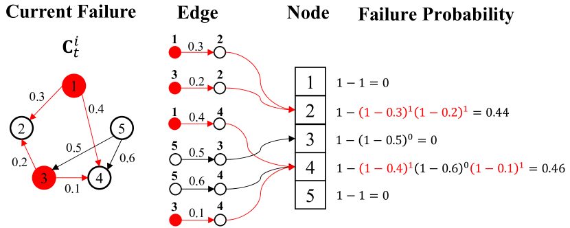
Figure 2: Traversing the edge list to calculate the failure probability

4.2 Graph validation

In graph validation, the second order term ${|{V^{{\cal M}\cup{\cal I}}}|(|{V^{{\cal M}\cup{\cal I}}}|+|{\mathcal{E}^{{\cal M}\cup{\cal I}}}|)}$ is due to checking the corresponding paths on every node in the network. However, considering the tripartite structure of ICI networks and since every iteration of the M-H algorithm only adds or removes one edge, the following theorem is proposed to guarantee that constraints (1)-(6) are validated in linear time.

Theorem 1

Let $\overrightarrow{\bm{A}}^{\prime},\overleftarrow{\bm{A}}^{\prime}$ denote the adjacency list and the reversed adjacency list of the proposed graph $\bm{G}^{\prime}$ after adding or removing the link (i, j) selected from the feasible set $\mathcal{S}$. Given that the graph $\bm{G}$ in the last iteration of the M-H algorithm has already satisfied constraints (1)-(9) and the current proposed graph $\bm{G}^{\prime}$ has already satisfied constraints (7)-(8), we claim that $\bm{G}^{\prime}$ satisfies constraints (1)-(6), (9) if and only if $\overrightarrow{\bm{A}}^{\prime}_{i}\neq\{\}$ and $\overleftarrow{\bm{A}}^{\prime}_{j}\neq\{\}$.

The proof of Theorem 1 is shown in Appendix C. Theorem 1 indicates that we can validate the proposed topology by only checking the out-degree of the heading node $i$ and the in-degree of the tailing node $j$, which only takes linear time ${\mathcal{O}(|{V^{{\cal M}\cup{\cal I}}}|+|{\mathcal{E}^{{\cal M}\cup{\cal I}}}|)}$.

4.3 Tie-No-Tie sampler

The third technique we employ to improve the sampling efficiency is to replace the random sampler at step 10 in Alg. 1 with the ’tie-no-tie’ (TNT) sampler [9, 42]. The random sampler selects pairs of nodes with equal probability, resulting in a higher frequency of proposing node pairs with non-edges (edges not present in the network) and adding the corresponding edges then proposing node pairs with edges and removing the corresponding edges in sparse graphs. However, the newly added edges are likely to be rejected due to the violation of constraints (1)-(9) or the generation of a network topology discouraged by the cascading failure data. Conversely, the TNT sampler first selects the set of edges or the set of non-edges with equal probability, and then changes a random node-pair in that set, which increases the frequency of removing edges in the proposal. Since removing edges are more likely to be accepted due to graph sparsity, the sampling efficiency is improved.

5 Numerical experiments

In this section, we apply the proposed Bayesian approach to one synthetic and two real-world ICIs. In the first case study, we design five methods from different combinations of the infrastructure-dependent proposal and different computational optimization techniques (Table I). By comparing the performance of these methods on reconstructing the synthetic system of ICI networks, we select the best method and apply it to two systems of real-world ICIs.

5.1 Synthetic networks

The synthetic system contains three blocks corresponding to water, power, and gas networks, each of which has three hierarchical levels corresponding to supply, transmission, and demand facilities (Fig. 3). All three networks have two supply nodes, three transmission nodes, and five demand nodes. The interdependency across networks is simulated using the approach for Synthetic Interdependent Critical Infrastructure Networks (SICIN) in [6], which requires as input the degree distribution extracted from real-world infrastructures of the same type. Two types of interdependencies are considered: 1) pumping stations require electricity from 12kV substations for pumping water from nearby rivers and 2) power gate stations depend on water from water delivery stations for cooling purposes; gas gate stations require electricity from 12kV substations for extracting natural gas from underground while power gate stations depend on natural gas from gas delivery stations for generating electricity. Both of the two interdependencies are considered by accounting for the distance between each facility. We denote the water-power-gas SICIN that we aim to reconstruct as $\bm{A}^{*}$ hereafter. The cascading failure data $\bm{C}$ is simulated using the SI epidemic model, the ratio of the initial failed nodes is set to $0.2$ and the probability of failure propagation $q$ in Eq. (2.2) is set to $0.4$ to get sufficient cascading failure data, which is aligned with prior work in the literature [9]. To demonstrate the dependency of the performance of reconstructing network topology on the amount of cascading data $\bm{C}$ we design three experiments: (i) $E_{5}^{5}$: five cascading failure scenarios with at least five time steps each (ii) $E_{5}^{15}$: 15 cascading failure scenarios with at least five time steps (iii) $E_{5}^{40}$: 40 cascading failure scenarios with at least five time steps. All three experiments are performed with and without considering infrastructure-dependent proposals.

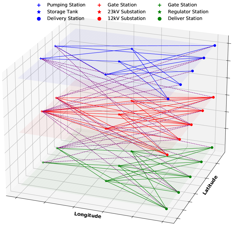
Figure 3: The water-power-gas SICIN. Solid lines represent links within a network while dashed lines represent interdependent links between networks.

Since the average degree is the basic metric for the connectivity and density of the network which affects network features such as the clustering coefficient and the diameter [43], we select the average degree as the representative network feature and draw its trace plot to validate the convergence of the M-H algorithm as shown in Figs. 4 and 5. Regardless of whether we consider the infrastructure-dependent proposal, the average degree of the reconstructed network in $E_{5}^{40}$ (green chain) is closer to the target value (black dashed line) than that in $E_{5}^{5}$ and $E_{5}^{15}$ (blue and orange chains). This outcome is primarily driven by the cascading failure data where the experiment with larger cascading failure scenarios and longer time steps in $E_{5}^{40}$ contains more node-pair information that covers a wider range of network topology than the data with fewer scenarios and shorter time steps in $E_{5}^{5},E_{5}^{15}$. Therefore, in $E_{5}^{40}$, the posterior of these edges is updated with more data of the corresponding node pairs, drawing the distribution closer to the target posterior. Also, when compared to the first two experiments, the value of the average degree converges to the target with fewer iterations in $E_{5}^{40}$, i.e., fewer iterations at the warm-up stage.

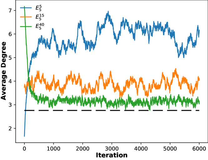
Figure 4: Average degree trace plot without infrastructure-dependent proposal

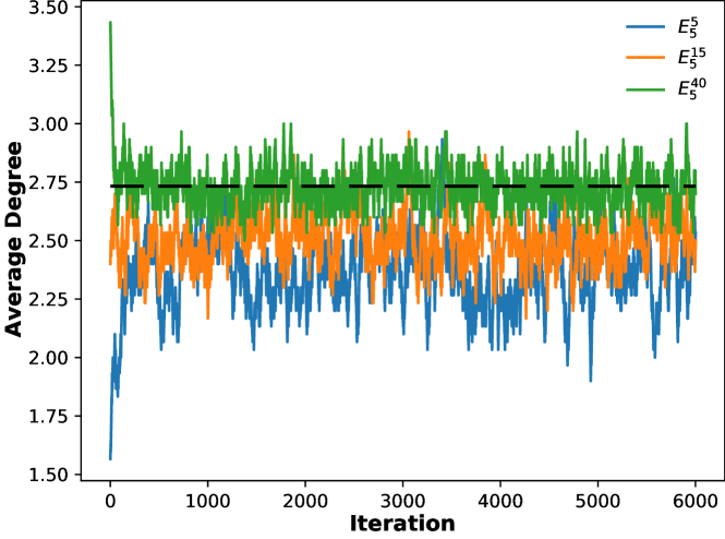
Figure 5: Average degree trace plot with infrastructure-dependent proposal

Comparing Figs. 4 and 5, we can observe that the average degree of the reconstructed network with infrastructure-dependent proposal converges more quickly and closer to the target value than that without infrastructure-dependent proposal in all three experiments. Since infrastructure-dependent proposal exerts extra topological constraints on the proposed network to generate more realistic candidate network topologies, it improves both the accuracy and the computational efficiency.

Next, we evaluate the accuracy of network reconstruction using adjacency matrix. Suppose that the set of networks in the posterior distribution is $\mathcal{A}$, the edge probability $p_{ij}$ for each pair of nodes $(i,j)$ is defined as the ratio of the number of graphs with the edge between $i,j$, $|\{{\mathbf{A}\in\mathcal{A}}:\mathbf{A}_{ij}=1\}|$, and the total number of graphs in the posterior, $|\mathcal{A}|$, as follows

$${p_{ij}}=\frac{|\{{\mathbf{A}\in\mathcal{A}}:\mathbf{A}_{ij}=1\}|}{|\mathcal{A}|}.$$ (11)

The edge probability for each pair of nodes in the network is displayed on the heatmap of the adjacency matrix shown in Fig. 6. In the first row of Fig. 6, a number of noisy edges that are not present in the real networks are proposed and shown in blank areas. In contrast, when using the infrastructure-dependent proposal (shown in the second row of Fig. 6), the heatmap of the adjacency matrix conforms to the block structure in the original network. Furthermore, since ${E}_{5}^{40}$ uses more cascading failure data to update the network topology, we have higher confidence in the predicted edges. Therefore, the heatmap of the adjacency matrix is darker in $E_{5}^{40}$ than in the other two experiments, indicating higher edge probability.

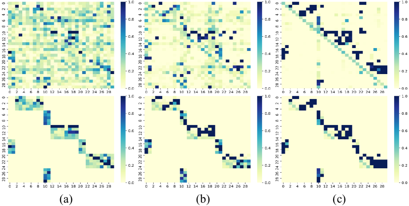
Figure 6: The heatmap of the adjacency matrix reconstructed without (the first row) and with (the second row) infrastructure-dependent proposal under three experiment settings $E_{5}^{5}$ (a), $E_{5}^{15}$ (b), and $E_{5}^{40}$ (c).

We now show the accuracy of the proposed network reconstruction approach. We set a probability threshold $p$ and classify node pairs into two categories: node pair connected by an edge if $p_{ij}\geq p$ and node pair not connected if $p_{ij}<p$. We further count the number of edges for each pair of nodes that are correctly classified and compute the F1-score which is the harmonic mean of precision and recall. The precision-recall curve is plotted in Figs. 18 and 19 in Appendix E. For each of the three experiments, the best F1-score is 0.44, 0.53, and 0.84 for experiments without infrastructure-dependent proposal, and 0.72, 0.85, and 0.95 for experiments with infrastructure-dependent proposal. This outcome is consistent with the previous observation that the accuracy of the reconstructed network improves with additional cascading data. In addition, our infrastructure-dependent proposal significantly improves the performance of reconstructing networks using the same amount of cascading failure data.

To demonstrate the computational performance of incorporating three optimization techniques, we devise five methods by combining different techniques and the infrastructure-dependent proposal. The details of the five methods are outlined in Table I where the checkmark denotes that the corresponding method uses the corresponding technique. ”IP” refers to using infrastructure-dependent proposal and ”Validation” refers to validating the proposed graph according to Theorem 1. We implement each of the five methods 10 times to reconstruct the synthetic networks and report their averaged reconstructing time and F1-score in Fig. 7. In each run, we propose 3000 samples and use the first 2000 samples as warm-ups.

TABLE I: The configuration of five methods for constructing ICIs.

Method	IP	TNT	Edgelist	Validation
M-1	✓	✓	✓	✓
M-2	✓	✓	✓
M-3	✓	✓
M-4	✓
M-5

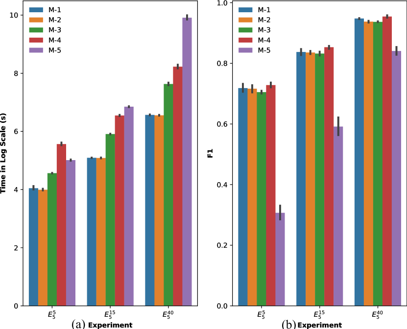
Figure 7: The time (a) and the F1-score (b) of reconstructing the synthetic networks using the five methods.

In Fig. 7(a), M-1 (blue) and M-2 (orange) have the shortest running time and the difference in running time between M-1, M-2 and the other three methods becomes larger as the amount of data increases from $E_{5}^{5}$ to $E_{5}^{40}$, indicating that traversing edge lists rather than adjacency matrix to calculate the likelihood significantly reduces the computational load and this reduction is significant when more failure data is used. The comparable running time between M-1 and M-2 indicates that applying graph validation according to Theorem 1 brings nearly no improvement in computational efficiency. This is because proposing networks by removing edges in TNT sampler can easily generate pairs of disconnected nodes and once we find such pairs of nodes, constraints (1)-(6) are broken and we save the time that would be otherwise needed to check other pairs of nodes. Comparing M-3 (green) and M-4 (red), replacing the random sampler with the TNT sampler reduces the computational load because the TNT sampler proposes more valid topological variation by removing edges rather than adding invalid edges that would be later rejected. The running time of M-4 (red) is greater than that of M-5 (purple) in $E_{5}^{5}$ while it is less in $E_{5}^{15},E_{5}^{40}$. Given the smaller amount of cascading failure data in $E_{5}^{5}$, the proposed networks can be easily accepted without applying the infrastructure-dependent proposal to check any topological constraint in advance. Therefore, the sampling process is completed in a shorter time in M-5 where no extra operations on checking the network topology are required. However, for larger cascading failure data in $E_{5}^{15}$ and $E_{5}^{40}$ and without verifying the network topology for constraints (1)-(9) in advance, the topology candidates proposed by the random sampler are more likely to be rejected as they are not supported by the cascading failure data (low likelihood). Therefore, the time spent on proposing such invalid samples is compensated by the time for checking the topological constraints, leading to shorter time in M-4 than M-5 for $E_{5}^{15}$ and $E_{5}^{40}$. In Fig. 7(b), the first four methods lead to roughly the same and better F1-score than M-5, which demonstrates the power of applying infrastructure-dependent proposals. However, M-4 which applies the random sampler is slightly better than the previous three methods M-1, M-2, M-3 that use the TNT sampler because some edges that are present in the target network have already been removed by the TNT sampler in M-1, M-2, M-3. The random sampler has a higher chance to add edges than the TNT sampler and thus is more likely to recover those edges that should exist in the target network but have already been removed. The running times of different experiments are provided in Tables II and III. Considering the trade-off between the running time and the reconstructing accuracy, M-1 is selected to be used in the following two real-world case studies.

TABLE II: The average F1-score of the five methods

Method	$E_{5}^{5}$	$E_{5}^{15}$	$E_{5}^{40}$
M-1	0.718	0.837	0.948
M-2	0.716	0.836	0.938
M-3	0.705	0.832	0.937
M-4	0.728	0.853	0.954
M-5	0.307	0.591	0.841

TABLE III: The average running time (s) of the five methods

Method	$E_{5}^{5}$	$E_{5}^{15}$	$E_{5}^{40}$
M-1	57.608	162.836	712.096
M-2	54.257	161.850	702.410
M-3	95.876	368.205	2067.501
M-4	261.652	697.319	3762.572
M-5	150.339	944.409	20305.656

5.2 Interdependent power, water, and gas networks in Shelby County

The experiments demonstrating the performance improvement brought by the infrastructure-dependent proposal have thus far only considered synthetic infrastructure networks. Therefore, we apply the proposed method to reconstruct real-world ICIs. The first case study considers the gas-power-water of Shelby County, Tennessee, Fig. 8. Since the size of these networks is larger than the synthetic networks, we increase the amount of cascading failure data to ensure a good performance of network reconstruction. The cascading failure data $E_{20}^{40}$ contains 20 cascading failure scenarios, each with 40 failure sequences. The constant probability value is taken from $0.1$ to $0.9$ with interval of $0.1$ to represent the low, middle and high probability of failure propagation. The F1-score and time of reconstructing the system of Shelby County infrastructure networks with different failure propagation probabilities are shown in Fig. 9.

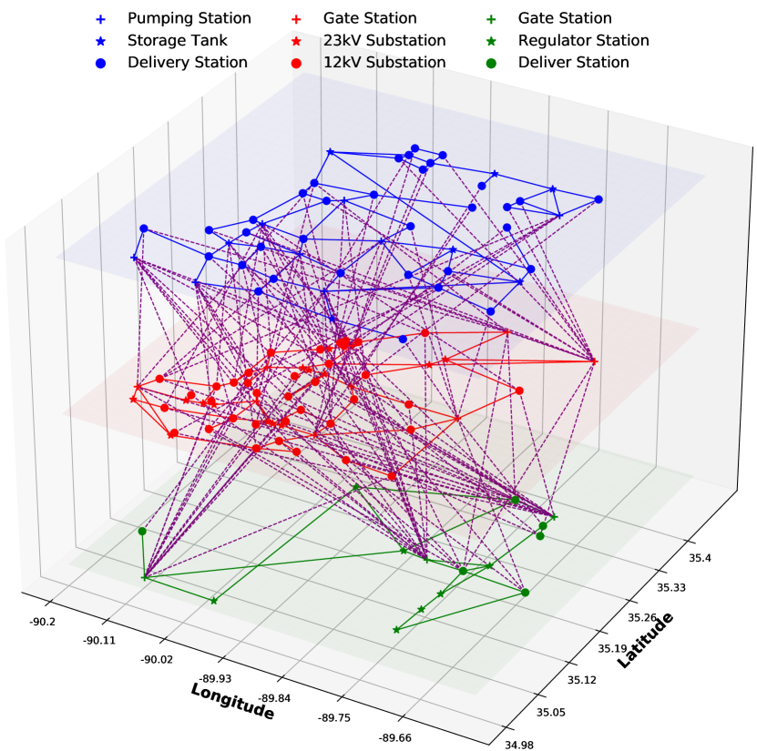
Figure 8: Interdependent gas-power-water networks of Shelby County

For the computation time, since generating network topology used for initiating the reconstruction process establishes invalid edges that do not belong to the target network, the following reconstruction process is to remove these invalid edges by proposing corresponding edge removal. However, since the likelihood of the network topology after removing these invalid edges becomes lower than the original network under the case of high probability of failure propagation, the proposal that removing these invalid edges is more likely to be rejected. Therefore, achieving the same number of posterior samples requires more time in the high probability of failure propagation than in the low one, as observed by the increasing reconstructing time with the increase of the probability of failure propagation. For the F1-score, a high probability of failure propagation prompts adding more edges between consequential failed nodes and the reconstructed network becomes sparser than the target one. Conversely, a very low probability prompts removing more unnecessary edges and the reconstructed network becomes denser than the target one. Both of the above two situations cause low reconstructing resolution and as observed in Fig. 9, the peak F1-score appears when the probability of failure propagation is around 0.4.

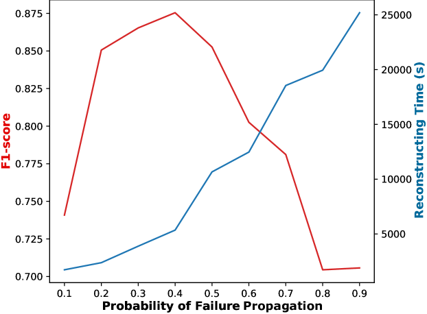
Figure 9: F1-score and time of reconstructing Shelby County networks. Solid lines represent links within a network while dashed lines represent interdependent links.

5.3 Interdependent power and water networks in Ideal City

The second case study considers the system of interdependent power and water networks (Fig. 10) extracted from a virtual city that mimics a typical Italian building stock with geographic boundaries spanning the city of Turin, Italy. The data was provided by [44] and processed to obtain subgraphs of the power and water networks. The water distribution network has one supply node (pumping station), 10 transmission nodes (storage tanks), and 67 demand nodes (delivery stations) while the power network consists of one supply node (gate station), 10 transmission nodes (intermediate stations), and 61 demand nodes (delivery substations). The geographical locations of facilities in these two networks are reorganized using the simulated annealing simulation algorithm based on the population distribution in Italy [45]. Since the topology of this network is more tree-like than the networks in the previous two case studies, the cascading failure is more difficult to propagate, leading to shorter cascading failure sequences. To obtain a reasonably good performance of network reconstruction, we increase the number of cascading scenarios to 100, each of which has at least 12 failure sequences. The F1-score of network reconstruction with different parameters is presented in Fig. 11.

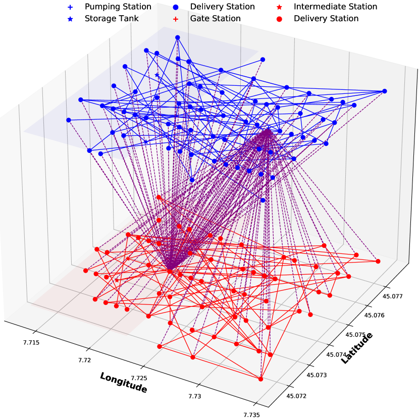
Figure 10: The interdependent gas-power-water networks of Ideal City. Solid lines represent links within a networks while dashed lines represent interdependent links.

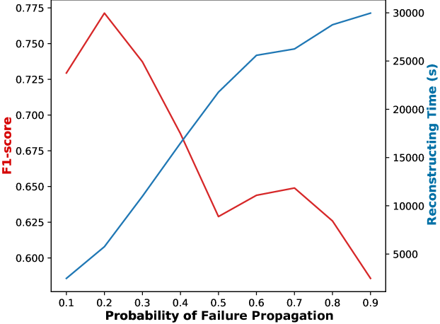
Figure 11: F1-score and time of reconstructing interdependent power and water networks in the Ideal City.

Similar to the observation in the second case study, the reconstructing time increases as the probability of failure propagation increases because the proposals of removing the invalid edges are more likely to be rejected. However, the peak of the F1-score appears when the probability of failure propagation is around 0.2, which is different from the previous case study. This indicates that the probability of failure propagation that achieves the best reconstructing performance depends on the particular topology of the ICI to be reconstructed. Another observation is that even though the number of the cascading scenarios used here is much greater than the previous case study, the best F1-score (0.775) is less than the best F1-score of the previous case study (0.875). This is because cascading failure is more difficult to propagate in the networks in Ideal City that only have two tree structures, therefore less information about the network topology is encoded in the cascading failure sequences than the previous case study.

6 Conclusion

This paper presents a Bayesian approach for reconstructing the topology of systems of ICI networks based on cascading failure data. The HSBM is used to capture the clustering and hierarchical structure of ICIs. The computational complexity resulting from the exponential growth of the potential topology is addressed by a new infrastructure-dependent proposal that takes into account the topological constraints of ICIs. Furthermore, we propose three techniques to significantly improve the sampling efficiency. Results of three case studies demonstrate the effectiveness and transferability of the proposed approach.

Future work can be carried out to investigate the influence of cascading failure data and the network structure on the reconstruction performance. While the proposed approach uses the SI epidemic model to simulate cascading failures in infrastructures, future work can explore other types of failure simulation models, such as susceptible-infected-susceptible (SIS), susceptible–infected–recovered (SIR), and their stochastic variants. In the last case study we demonstrate that the performance of reconstructing the network topology based on the cascading failure data varies from network to network and heavily relies on the topology of the networks. As such, further research can help identify the network topology for which the proposed reconstruction method is best suited.

References

- [1] B. D. Fath, U. M. Scharler, R. E. Ulanowicz, and B. Hannon, “Ecological network analysis: Network construction,” Ecological Modelling, vol. 208, no. 1, pp. 49–55, 2007.
- [2] P. Sharma, D. J. Bucci, S. K. Brahma, and P. K. Varshney, “Communication network topology inference via transfer entropy,” IEEE Transactions on Network Science and Engineering, vol. 7, no. 1, pp. 562–575, 2019.
- [3] I. Brugere, B. Gallagher, and T. Y. Berger-Wolf, “Network structure inference, a survey: Motivations, methods, and applications,” ACM Computing Surveys (CSUR), vol. 51, no. 2, pp. 1–39, 2018.
- [4] C.-W. Ten, C.-C. Liu, and G. Manimaran, “Vulnerability assessment of cybersecurity for scada systems,” IEEE Transactions on Power Systems, vol. 23, no. 4, pp. 1836–1846, 2008.
- [5] W. L. Hamilton, R. Ying, and J. Leskovec, “Representation learning on graphs: Methods and applications,” arXiv preprint arXiv:1709.05584, 2017.
- [6] Y. Wang, J.-Z. Yu, and H. Baroud, “Generating synthetic systems of interdependent critical infrastructure networks,” IEEE Systems Journal, vol. 16, no. 2, pp. 3191–3202, 2022.
- [7] N. Ahmad, M. Chester, E. Bondank, M. Arabi, N. Johnson, and B. L. Ruddell, “A synthetic water distribution network model for urban resilience,” Sustainable and Resilient Infrastructure, pp. 1–15, 2020.
- [8] C. Zhai, T. Y.-j. Chen, A. G. White, and S. D. Guikema, “Power outage prediction for natural hazards using synthetic power distribution systems,” Reliability Engineering & System Safety, vol. 208, p. 107348, 2021.
- [9] C. Gray, L. Mitchell, and M. Roughan, “Bayesian inference of network structure from information cascades,” IEEE Transactions on Signal and Information Processing over Networks, vol. 6, pp. 371–381, 2020.
- [10] A. Braunstein, A. Ingrosso, and A. P. Muntoni, “Network reconstruction from infection cascades,” Journal of the Royal Society Interface, vol. 16, no. 151, p. 20180844, 2019.
- [11] A. Vajdi and C. M. Scoglio, “Identification of missing links using susceptible-infected-susceptible spreading traces,” IEEE Transactions on Network Science and Engineering, vol. 6, no. 4, pp. 917–927, 2018.
- [12] Y. Zhao, Y.-J. Wu, E. Levina, and J. Zhu, “Link prediction for partially observed networks,” Journal of Computational and Graphical Statistics, vol. 26, no. 3, pp. 725–733, 2017.
- [13] K. Huang, Z. Wang, and M. Jusup, “Incorporating latent constraints to enhance inference of network structure,” IEEE Transactions on Network Science and Engineering, vol. 7, no. 1, pp. 466–475, 2018.
- [14] H.-F. Zhang, F. Xu, Z.-K. Bao, and C. Ma, “Reconstructing of networks with binary-state dynamics via generalized statistical inference,” IEEE Transactions on Circuits and Systems I: Regular Papers, vol. 66, no. 4, pp. 1608–1619, 2018.
- [15] M. Wilinski and A. Y. Lokhov, “Scalable learning of independent cascade dynamics from partial observations,” arXiv preprint arXiv:2007.06557, 2020.
- [16] C. Jiang, J. Gao, and M. Magdon-Ismail, “True nonlinear dynamics from incomplete networks,” in Proceedings of the AAAI Conference on Artificial Intelligence, vol. 34, no. 01, 2020, pp. 131–138.
- [17] T. K. Dey, J. Wang, and Y. Wang, “Road network reconstruction from satellite images with machine learning supported by topological methods,” in Proceedings of the 27th ACM SIGSPATIAL International Conference on Advances in Geographic Information Systems, 2019, pp. 520–523.
- [18] A. Clauset, C. Moore, and M. E. Newman, “Hierarchical structure and the prediction of missing links in networks,” Nature, vol. 453, no. 7191, pp. 98–101, 2008.
- [19] A. Louni and K. Subbalakshmi, “Diffusion of information in social networks,” in Social Networking. Springer, 2014, pp. 1–22.
- [20] R. G. Little, “Controlling cascading failure: Understanding the vulnerabilities of interconnected infrastructures,” Journal of Urban Technology, vol. 9, no. 1, pp. 109–123, 2002.
- [21] J. H. Parmelee and S. L. Bichard, Politics and the Twitter revolution: How tweets influence the relationship between political leaders and the public. Lexington Books, 2011.
- [22] S. Pajevic and D. Plenz, “Efficient network reconstruction from dynamical cascades identifies small-world topology of neuronal avalanches,” PLoS Computational Biology, vol. 5, no. 1, p. e1000271, 2009.
- [23] A. Grover and J. Leskovec, “node2vec: Scalable feature learning for networks,” in Proceedings of the 22nd ACM SIGKDD International Conference on Knowledge Discovery and Data Mining, 2016, pp. 855–864.
- [24] W. Hamilton, Z. Ying, and J. Leskovec, “Inductive representation learning on large graphs,” in Advances in Neural Information Processing Systems, 2017, pp. 1024–1034.
- [25] T. N. Kipf and M. Welling, “Semi-supervised classification with graph convolutional networks,” arXiv preprint arXiv:1609.02907, 2016.
- [26] E. K. Kao, S. T. Smith, and E. M. Airoldi, “Hybrid mixed-membership blockmodel for inference on realistic network interactions,” IEEE Transactions on Network Science and Engineering, vol. 6, no. 3, pp. 336–350, 2018.
- [27] T. P. Peixoto, “Network reconstruction and community detection from dynamics,” Physical Review Letters, vol. 123, no. 12, p. 128301, 2019.
- [28] J.-G. Young, G. T. Cantwell, and M. Newman, “Bayesian inference of network structure from unreliable data,” Journal of Complex Networks, vol. 8, no. 6, p. cnaa046, 2020.
- [29] F. Scarselli, M. Gori, A. C. Tsoi, M. Hagenbuchner, and G. Monfardini, “The graph neural network model,” IEEE Transactions on Neural Networks, vol. 20, no. 1, pp. 61–80, 2008.
- [30] M. Chen, J. Zhang, Z. Zhang, L. Du, Q. Hu, S. Wang, and J. Zhu, “Inference for network structure and dynamics from time series data via graph neural network,” arXiv preprint arXiv:2001.06576, 2020.
- [31] M. F. Ochs and E. J. Fertig, “Matrix factorization for transcriptional regulatory network inference,” in 2012 IEEE Symposium on Computational Intelligence in Bioinformatics and Computational Biology (CIBCB). IEEE, 2012, pp. 387–396.
- [32] A. M. Madni, “A systems perspective on compressed sensing and its use in reconstructing sparse networks,” IEEE Systems Journal, vol. 8, no. 1, pp. 23–27, 2013.
- [33] Z. Shen, W.-X. Wang, Y. Fan, Z. Di, and Y.-C. Lai, “Reconstructing propagation networks with natural diversity and identifying hidden sources,” Nature Communications, vol. 5, no. 1, pp. 1–10, 2014.
- [34] M. Gomez-Rodriguez, J. Leskovec, and A. Krause, “Inferring networks of diffusion and influence,” ACM Transactions on Knowledge Discovery from Data (TKDD), vol. 5, no. 4, pp. 1–37, 2012.
- [35] M. Wu, J. Chen, S. He, Y. Sun, S. Havlin, and J. Gao, “Discrimination universally determines reconstruction of multiplex networks,” arXiv preprint arXiv:2001.09809, 2020.
- [36] M. Ouyang, “Review on modeling and simulation of interdependent critical infrastructure systems,” Reliability Engineering & System safety, vol. 121, pp. 43–60, 2014.
- [37] O. Yagan, D. Qian, J. Zhang, and D. Cochran, “Optimal allocation of interconnecting links in cyber-physical systems: Interdependence, cascading failures, and robustness,” IEEE Transactions on Parallel and Distributed Systems, vol. 23, no. 9, pp. 1708–1720, 2012.
- [38] Y. Zhang and O. Yağan, “Robustness of interdependent cyber-physical systems against cascading failures,” IEEE Transactions on Automatic Control, 2019.
- [39] J. M. Adam, F. Parisi, J. Sagaseta, and X. Lu, “Research and practice on progressive collapse and robustness of building structures in the 21st century,” Engineering Structures, vol. 173, pp. 122–149, 2018.
- [40] S. H. Cheung and J. L. Beck, “Bayesian model updating using hybrid Monte Carlo simulation with application to structural dynamic models with many uncertain parameters,” Journal of Engineering Mechanics, vol. 135, no. 4, pp. 243–255, 2009.
- [41] J.-Z. Yu, M. Whitman, A. Kermanshah, and H. Baroud, “A hierarchical bayesian approach for assessing infrastructure networks serviceability under uncertainty: A case study of water distribution systems,” Reliability Engineering & System Safety, p. 107735, 2021.
- [42] D. Lusher, J. Koskinen, and G. Robins, Exponential random graph models for social networks: Theory, methods, and applications. Cambridge University Press, 2013.
- [43] M. A. Serrano and M. Boguná, “Tuning clustering in random networks with arbitrary degree distributions,” Physical Review E, vol. 72, no. 3, p. 036133, 2005.
- [44] S. Marasco, A. Cardoni, A. Z. Noori, O. Kammouh, M. Domaneschi, and G. P. Cimellarof, “Integrated platform to assess seismic resilience at the community level,” Sustainable Cities and Society, p. 102506, 2020.
- [45] Italian National Institute of Statistics, “Resident population,” http://demo.istat.it/, 2019.