On the Effectiveness of Parameter-Efficient Fine-Tuning

Abstract

Fine-tuning pre-trained models has been ubiquitously proven to be effective in a wide range of NLP tasks. However, fine-tuning the whole model is parameter inefficient as it always yields an entirely new model for each task. Currently, many research works propose to only fine-tune a small portion of the parameters while keeping most of the parameters shared across different tasks. These methods achieve surprisingly good performance and are shown to be more stable than their corresponding fully fine-tuned counterparts. However, such kind of methods is still not well understood. Some natural questions arise: How does the parameter sparsity lead to promising performance? Why is the model more stable than the fully fine-tuned models? How to choose the tunable parameters? In this paper, we first categorize the existing methods into random approaches, rule-based approaches, and projection-based approaches based on how they choose which parameters to tune. Then, we show that all of the methods are actually sparse fine-tuned models and conduct a novel theoretical analysis of them. We indicate that the sparsity is actually imposing a regularization on the original model by controlling the upper bound of the stability. Such stability leads to better generalization capability which has been empirically observed in a lot of recent research works. Despite the effectiveness of sparsity grounded by our theory, it still remains an open problem of how to choose the tunable parameters. Currently, the random and rule-based methods do not utilize task-specific data information while the projection-based approaches suffer from the projection discontinuity problem. To better choose the tunable parameters, we propose a novel Second-order Approximation Method (SAM) which approximates the original problem with an analytically solvable optimization function. The tunable parameters are determined by directly optimizing the approximation function. We conduct extensive experiments on several tasks. The experimental results show that our proposed SAM model outperforms many strong baseline models and it also verifies our theoretical analysis.

1 Introduction

Fine-tuning the model parameters for a specific task on a pre-trained model Peters et al. (2018); Kenton and Toutanova (2019); Lan et al. (2020); Radford et al. (2018, 2019); Liu et al. (2019); Brown et al. (2020); Lewis et al. (2020); Raffel et al. (2020) has become one of the most promising techniques for NLP in recent years. It achieves state-of-the-art performance on most of the NLP tasks. However, as the parameter number grows exponentially to billions Brown et al. (2020) or even trillions Fedus et al. (2021), it becomes very inefficient to save the fully fine-tuned parameters He et al. (2021a) for each downstream task. Many recent research works propose a parameter-efficient Houlsby et al. (2019); Zaken et al. (2021); He et al. (2021a) way to solve this problem by tuning only a small part of the original parameters and storing the tuned parameters for each task.

Apart from the efficiency of the parameter-efficient models, it has also been observed in many recent research works that the parameter-efficient methods achieve surprisingly good performance. These models are more stable He et al. (2021b); Lee et al. (2019); Houlsby et al. (2019); Zaken et al. (2021); Sung et al. (2021); Liu et al. (2021); Ding et al. (2022) and even achieve better overall scores than the fully fine-tuned models Lee et al. (2019); Houlsby et al. (2019); Zaken et al. (2021); Sung et al. (2021); Liu et al. (2021); Xu et al. (2021); Guo et al. (2021); He et al. (2021a); Ding et al. (2022) on some tasks. Currently, it remains unclear why the parameter-efficient models can improve the stability and performance in many prevalent works. In this paper, we first categorize the existing methods into three categories (i.e. random approaches, rule-based approaches, and projection-based approaches) depending on how they choose the tunable parameters. Then, we define the generalized sparse fine-tuned model and illustrate that most of the existing parameter-efficient models are actually a sparse fine-tuned model. Afterwards, we introduce the widely used pointwise hypothesis stability of the sparse fine-tuned model and show theoretically that the sparsity actually controls the upper bound of the stability. Based on the stability analysis, we further give a theoretical analysis of the generalization bound for the sparse fine-tuned model.

Though promising results have been achieved by existing parameter-efficient models, it still remains a challenging problem to select suitable parameters as it is an NP-hard problem. Currently, the random Lee et al. (2019) and rule-based Zaken et al. (2021); Han et al. (2015a); Houlsby et al. (2019); Pfeiffer et al. (2020) approaches propose to optimize fixed parameters. These methods are straightforward and easy to implement but they do not utilize task-specific data information. To solve this problem, the projection-based approaches Mallya et al. (2018); Guo et al. (2021); Xu et al. (2021) propose to calculate a score for each parameter based on the data and project the scores onto the parameter selection mask’s feasible region (an $L_{0}$ ball). However, as the feasible region is non-convex, we will show that such projection suffers from the projection discontinuity problem which makes the parameter selection quite unstable. To solve these problems, we propose a novel Second-order Approximation Method (SAM) to approximate the NP-hard optimization target function with an analytically solvable function. Then, we directly choose the parameters based on the optimal value and optimize the parameters accordingly. We conduct extensive experiments to validate our theoretical analysis and our proposed SAM model.

Our contributions can be summarized as follows: 1) We propose a new categorization scheme for existing parameter-efficient methods and generalize most of these methods with a unified view called the sparse fine-tuned model. 2) We conduct a theoretical analysis of the parameter-efficient models’ stability and generalization. 3) We propose a novel SAM model to choose the suitable parameters to optimize. 4) We conduct extensive experiments to verify our theoretical analysis and the SAM model.

2 Unified View of Parameter Efficient Fine-tuning

In this section, we first define the unified sparse fine-tuned model which is simpler and easier for theoretical analysis. Then, we give a unified form of the optimization target. Afterwards, similar to previous works Ding et al. (2022); He et al. (2021a); Mao et al. (2021), we categorize these models into three categories based on how the parameters are chosen. Finally, we show that all the models are sparse fine-tuned model.

2.1 Sparse Fine-tuned Model

We first give the definition of sparse fine-tuned model as well as a unified optimization target. The equivalent model is also defined to help understand the models with modified structures.

Definition 1 ($p$-Sparse Fine-tuned Model).

Given a pre-trained model $\operatorname{\mathcal{M}}^{0}$ with parameters $\theta^{0}$, if a fine-tuned model $\operatorname{\mathcal{M}}$ with parameters $\theta$ has the same structure as $\operatorname{\mathcal{M}}^{0}$ such that $\|\theta-\theta^{0}\|_{0}\leq p\dim(\theta),p\in(0,1)$, we say the model $\operatorname{\mathcal{M}}$ is a $p$-sparse fine-tuned model with the sparsity $p$.

Many previous works propose different methods of selecting proper parameters to fine-tune. We unify these methods by denoting $M$ as a mask matrix on the parameters and the parameter $\theta$ can be denoted as $\theta=\theta^{0}+M\Delta\theta$, where $\Delta\theta$ is the difference vector. For a fixed sparsity coefficient $p$, the sparse fine-tuned model is trying to solve the following problem:

$$\min_{\Delta\theta,M}\operatorname{\mathcal{L}}(\theta^{0}+M\Delta\theta)$$ (1)

$$s.t.\ \ \ \ \|M\|_{0}= \lfloor mp\rfloor;\ \ \ \ M_{ij}=0,\forall i\neq j;\ \ \ \ M_{ii}\in\{0,1\},$$

where $\lfloor\cdot\rfloor$ is the floor function, $m=\dim(\theta)$ is the parameter number, $M\in\{0,1\}^{m\times m}$ is the parameter mask matrix with the diagonal equal to 0 or 1 while other elements are equal to 0 and $\operatorname{\mathcal{L}}$ is the loss function. We will show that most of the existing methods are sparse fine-tuned models. However, in Definition 1, we assume that the fine-tuned model $\operatorname{\mathcal{M}}$ has the same structure as $\operatorname{\mathcal{M}}^{0}$. This assumption hinders us from analyzing many models that alter the structure including Adapter Houlsby et al. (2019); Pfeiffer et al. (2020); Rücklé et al. (2021); He et al. (2021b), LoRA Hu et al. (2022), and etc. We define the notion of equivalent model to solve this problem.

Definition 2 (Equivalent Model).

Given a pre-trained model $\operatorname{\mathcal{M}}^{0}$ with parameters $\theta^{0}$, we say that a model $\tilde{\operatorname{\mathcal{M}}^{0}}$ with parameters $\tilde{\theta}^{0}$ is an equivalent model for model $\operatorname{\mathcal{M}}^{0}$ if $\forall x,\operatorname{\mathcal{M}}^{0}(x)=\tilde{\operatorname{\mathcal{M}}^{0}}(x)$.

Here, we do not require that the equivalent model shares the same structure as the original model. As a result, for models fine-tuned with additional structures (e.g. Adapter and LoRA), we can still get a sparse fine-tuned model with respect to an equivalent model $\tilde{\operatorname{\mathcal{M}}^{0}}$ instead of the original pre-trained model $\operatorname{\mathcal{M}}^{0}$. Therefore, our analysis for the sparse fine-tuned model is also applicable to them.

2.2 Parameter Efficient Fine-tuning as Sparse Fine-tuned Model

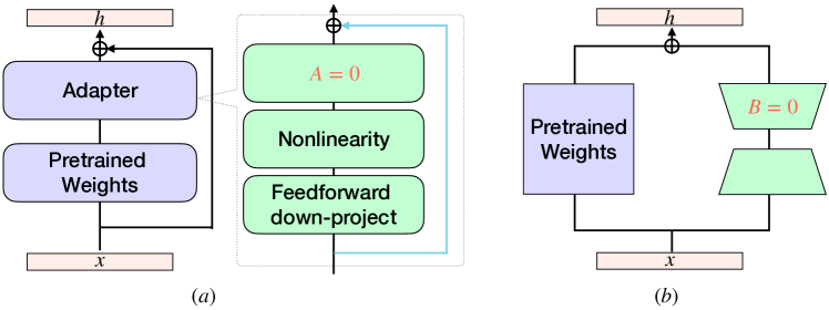
Figure 1: Equivalent model for Adapter (a) and LoRA (b).

Unfortunately, Problem (1) is NP-Hard due to the nonconvexity of the feasible region of the matrix $M$. Many existing methods propose to solve this problem by first estimating $M$ and then optimizing other parameters. Based on different strategies for choosing $M$, the methods can be divided into three categories, namely, random approaches, rule-based approaches, and projection-based approaches. We first give a general introduction of the prevalent parameter efficient fine-tuning methods in each category and then show that all of these methods are actually a sparse fine-tuned model. Then, in next section, we can prove our theory only based on properties in Definition 1 without refering to any specific model’s property.

2.2.1 Random Approaches

Random approaches include Random and Mixout models. These models randomly choose the parameters to be tuned. Such selection does not depend on the task-specific data information. Specifically, Random model is very straightforward by randomly selecting the parameters with respect to a given sparsity ratio and then training the selected parameters. Therefore, according to Definition 1, it is a sparse fine-tuned model. Mixout Lee et al. (2019) proposes to directly reset a portion of the fine-tuned model’s parameters to the pre-trained parameters with respect to a ratio. Therefore, according to Definition 1, it is a sparse fine-tuned model.

2.2.2 Rule-Based Approaches

The rule-based approaches include BitFit, MagPruning, Adapter, and LoRA. This kind of methods directly uses a pre-defined rule to fix the parameters to be tuned. It can be viewed as incorporating prior knowledge to recognize important features and can thus alleviate the problem of random approaches. However, the selection rules are still irrelevant to the specific data. Specifically, BitFit Zaken et al. (2021) only fine-tunes the bias-terms and achieves considerably good performance. Therefore, according to Definition 1, it is a sparse fine-tuned model with pre-defined tuning weights. MagPruning Han et al. (2015a, b); Lee et al. (2021); Lagunas et al. (2021) follows the idea that large weights are more important in the model. It ranks the weights by the absolute value and tunes the parameters with high absolute values. Therefore, according to Definition 1, it is a sparse fine-tuned model. Adapter Houlsby et al. (2019); Pfeiffer et al. (2020); Rücklé et al. (2021); He et al. (2021b); Karimi Mahabadi et al. (2021); Kim et al. (2021); Mahabadi et al. (2021) proposes to add an adapter layer inside the transformer layer. Therefore, the model structure is different from the original model. To make it easier to analyze, Adapter can be viewed as fine-tuning an equivalent model shown in Fig. 1 (a) which initializes the matrix $A$ as an all-zero matrix. The equivalent model has the same output as the original pre-trained model for arbitrary input while the structure is the same as the Adapter model. Therefore, fine-tuning the adapter model can be viewed as fine-tuning partial parameters of the equivalent model with the same structure. According to Definition 1, it is a sparse fine-tuned model with respect to the equivalent model. LoRA Hu et al. (2022); Karimi Mahabadi et al. (2021); Panahi et al. (2021) proposes to add a new vector calculated by recovering an hidden vector from a lower dimension space. The model is illustrated in Fig. 1 (b). It is interesting to notice that the original initialization makes the LoRA model already an equivalent model for the original pre-trained model as the matrix $B$ is set to 0. Therefore, according to Definition 1, fine-tuning a LoRA model can also be viewed as fine-tuning partial parameters of the equivalent model with the same structure.

2.2.3 Projection-Based Approaches

To utilize the task-specific data to help select the model’s tunable parameters, many researchers propose projection-based approaches including the DiffPruning, ChildPruning, and etc. These methods propose to choose the optimal parameter mask $M$ and optimize the parameters $\theta$ alternately to solve Problem (1). Specifically, they first relax $M$ as a continuous variable to get an optimized value and then project the optimized value onto the feasible region which can be denoted as $\hat{M}=\Pi_{\Omega}(M)=\arg\min_{\hat{M}\in\Omega}\|\hat{M}-M\|$, where $\Omega=\{M|\|M\|_{0}=\lfloor mp\rfloor;M_{ij}=0,\forall i\neq j;M_{ii}\in\{0,1\}\}$ and $\Pi_{\Omega}$ denotes the projection operator onto the feasible region $\Omega$ which is an $L_{0}$ ball. Specifically, DiffPruning Mallya et al. (2018); Sanh et al. (2020); Guo et al. (2021); Lagunas et al. (2021) proposes to model the parameter selection mask as a Bernoulli random variable and optimize the variable with a reparametrization method. It then projects the mask onto $M$’s feasible region $\Omega$ and do the optimization alternately. Therefore, according to Definition 1, it is also a sparse fine-tuned model. ChildPruning Xu et al. (2021); Mostafa and Wang (2019) proposes to iteratively train the full model parameters and then calculates the projected mask to find the child network. Therefore, it also agrees with the sparse fine-tuned model’s definition.

Projection Discontinuity Problem. Though projection-based methods can utilize task-specific data information, such kind of methods suffers from the projection discontinuity problem. Specifically, the feasible region $\Omega$ (the $L_{0}$ ball) of $M$ is non-convex. Therefore, it does not have the non-expansion property which is generally guaranteed for projection onto a closed convex set. As a result, a small perturbation on $M$ can lead to a totally different projection. For example, as illustrated in Fig. 2, suppose that $p=0.5$ and $M_{1}=\operatorname{diag}\{0.99,1\},M_{2}=\operatorname{diag}\{1,0.99\}$. Though $M_{1}\approx M_{2}$, we have $\Pi_{\Omega}(M_{1})=\operatorname{diag}\{0,1\}$ while $\Pi_{\Omega}(M_{2})=\operatorname{diag}\{1,0\}$, which is quite different. Consequently, the projection is very sensitive to the parameters updating noise. As a result, it is hard to keep consistent with the previous parameters selection which leads to a big change for the parameters selection. Such inconsistency will impair the overall performance.

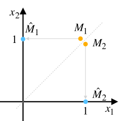
Figure 2: Projection discontinuity problem.

3 Theoretical Analysis of the Sparse Fine-tuned Model

Suppose that we have a pre-trained model $\operatorname{\mathcal{M}}^{0}$ with parameters $\theta^{0}$, we fine-tune the sparse fine-tuned model $\operatorname{\mathcal{M}}$ by updating only $\lfloor pm\rfloor$ parameters. We will first show that sparsity implies a regularization of the original model. Then, we prove that if a model is a sparse fine-tuned model, the model stability can benefit from the sparsity. Next, we give a theoretical analysis of the model generalization error bound and show that sparsity contributes to reducing the generalization error. It should be noted that in the proofs, we only use properties from Definition 1. Therefore, our theory is applicable to all model categories (random approaches, rule-based approaches, and projection-based approaches) that agrees with Definition 1.

3.1 Sparse Fine-tuned Model as a Regularizer

As analyzed in section 2.2, most of the models choose the parameter mask $M$ with different approaches and optimize the parameters $\theta$ accordingly. Here, we treat the matrix $M$ as a given parameter and denote $\theta=\theta^{0}+M\Delta\theta$. The sparse fine-tuned optimization in Problem (1) can be reformulated as:

$$\min_{\theta}\mathcal{L}(\theta)$$ (2)

$$s.t.\ \ \|(I -M)(\theta-\theta^{0})\|^{2}=0,$$

where $M=\operatorname{diag}\{M_{11},\cdots,M_{mm}\}$ is a diagonal matrix with $M_{ii}\in\{0,1\}$. By Lagrangian duality, solving Problem (2) is equivalent to solving the following problem:

$$\small\bar{L}=\min_{\theta}\max_{\lambda}\mathcal{L}(\theta)+\lambda\|(I-M)(\theta-\theta^{0})\|^{2}.$$ (3)

Then, we derive a new regularized problem with the following proposition.

Proposition 1.

Optimizing Problem (2) implies to optimizing the upper bound $\bar{L}$ of the following regularized problem:

$$L_{R}=\min_{\theta}\mathcal{L}(\theta)+\|(I-M)(\theta-\theta^{0})\|^{2}\leq\bar{L}.$$ (4)

The proof can be found in Appendix A.1. It can be concluded that optimizing Problem (2) is the same as optimizing the upper bound of the original loss function $\mathcal{L}(\theta)$ with a regularization term $\|(I-M)(\theta-\theta^{0})\|^{2}$. We will show later that such regularization contributes to the stability of the sparse fine-tuned model.

3.2 Stability Analysis

Stability has been studied in a lot of previous research works Bousquet and Elisseeff (2002); Shalev-Shwartz et al. (2010); Shalev-Shwartz and Ben-David (2014); Hardt et al. (2016); Kuzborskij and Lampert (2018); Charles and Papailiopoulos (2018); Fu et al. (2021) in many different forms. We focus on one of the commonly used notions, namely, the Pointwise Hypothesis Stability (PHS) which focuses on analyzing the change of model output after a training sample is removed. Following Charles and Papailiopoulos (2018), we denote the original training data as $S=\{z_{1},\cdots,z_{n}\}$ and the dataset without one sample as $S^{i}=S\backslash z_{i}=\{z_{1},\cdots,z_{i-1},z_{i+1},\cdots,z_{n}\}$, where $z_{i}$ is the $i$th training sample. We also define $i\sim U(n)$ as a sampling procedure from a uniform distribution with $n$ samples. $\operatorname{\mathcal{A}}(S)$ is defined as model parameters obtained by running algorithm $\operatorname{\mathcal{A}}$ on data $S$.

Definition 3 (Pointwise Hypothesis Stability, Bousquet and Elisseeff (2002)).

We say that a learning algorithm $\operatorname{\mathcal{A}}$ has pointwise hypothesis stability $\epsilon$ with respect to a loss function $\ell$, if

$$\small\mathbb{E}_{S,i\sim U(n)}[|\ell(\operatorname{\mathcal{A}}(S^{i}),z_{i})-\ell(\operatorname{\mathcal{A}}(S),z_{i})|]\leq\epsilon.$$ (5)

Here, $\ell(\theta,z_{i})$ is the single sample loss for $z_{i}$ when the model parameter is $\theta$. We assume that $\operatorname{\mathcal{A}}(S^{i})$ is close to $\operatorname{\mathcal{A}}(S)$. As $\operatorname{\mathcal{A}}(S)$ is the optimal solution, the Hessian matrix at $\operatorname{\mathcal{A}}(S)$ is a positive-semidefinite matrix. We can derive our bound for PHS in the following theorem.

Theorem 1 (Stability).

If the loss function $\ell$ is $\rho-$Lipschitz, $\operatorname{\mathcal{A}}(S^{i})$ is close to $\operatorname{\mathcal{A}}(S)$, the Hessian matrix $\nabla^{2}\mathcal{L}(\operatorname{\mathcal{A}}(S))$ at $\operatorname{\mathcal{A}}(S)$ is positive-semidefinite with a singular value decomposition $U\operatorname{diag}(\Lambda)U^{-1}$, $\Lambda=\{\Lambda_{1},\cdots,\Lambda_{m}\}$ and $\Lambda_{min}=\min\{\Lambda_{1},\cdots,\Lambda_{m}\}$, then the expectation of the loss $\mathbb{E}_{M}L_{R}$ has a pointwise hypothesis stability as:

$$\mathbb{E}_{S,i\sim U(n)}[|\ell(\operatorname{\mathcal{A}}(S^{i}),z_{i})-\ell(\operatorname{\mathcal{A}}(S),z_{i})|]\leq\frac{2\rho^{2}}{(\Lambda_{min}+2(1-p))n}.$$ (6)

The proof can be found in Appendix A.2. It can be observed from Theorem 1 that as the sparsity parameter $p$ decreases, the upper bound also decreases. Therefore, sparse models imply better stability which explains most of the empirical results observed in many recent works He et al. (2021b); Lee et al. (2019); Houlsby et al. (2019); Zaken et al. (2021); Sung et al. (2021); Liu et al. (2021); Ding et al. (2022). It should also be noted that if $p$ is small enough, the upper bound will not change significantly as $p$ continues to decrease. This is because in this case, the denominator is dominated by $\Lambda_{min}$ which is related to the landscape of the function. Empirically, if the sparsity is too small, the landscape will heavily depend on how the parameters are chosen and thus the stability is impaired.

3.3 Generalization Analysis

With the bound for the stability, we can then get the generalization error bound for the sparse fine-tuned model.

Theorem 2 (Generalization).

We denote the generalization error as $R(\operatorname{\mathcal{A}},S)=\mathbb{E}_{z}\ell(\operatorname{\mathcal{A}}(S),z)$ and the empirical error as $\hat{R}(\operatorname{\mathcal{A}},S)=\frac{1}{n}\sum_{i=1}^{n}\ell(\operatorname{\mathcal{A}}(S),z)$. Then, for some constant $C$, we have with probability $1-\delta$,

$$R(\operatorname{\mathcal{A}},S)\leq\hat{R}(\operatorname{\mathcal{A}},S)+\sqrt{\frac{C^{2}+\frac{24C\rho^{2}}{\Lambda_{min}+2(1-p)}}{2n\delta}}.$$ (7)

The proof can be found in Appendix A.3. This result shows that the generalization error upper bound becomes smaller as the fine-tuned parameters become sparser. Intuitively, if a model is stable, a perturbation makes less effect on the model and the model is less likely to overfit. It should be noted that the generalization error bound is determined by both the empirical error $\hat{R}(\operatorname{\mathcal{A}},S)$ and sparsity. Therefore, as the mask becomes sparser, even though the second term decreases, the training error $\hat{R}(\operatorname{\mathcal{A}},S)$ will possibly increase when the tunable parameters are not enough to fit the data. Consequently, as the sparsity decreases, the generalization error will first decrease and then increase. We will further examine this conjecture in experiments.

4 Second-order Approximation Method

In Section 3, we theoretically prove the effectiveness of sparsity in fine-tuning. However, it still remains a problem of how to choose the tunable parameters. As discussed in Section 2.2, the random and the rule-based approaches are robust to noise perturbation as the tunable parameters are fixed during training. However, these methods tune the same parameters on all kinds of tasks without utilizing the information from the task-specific data. On the other hand, the projection-based approaches solve this problem by getting full utilization of the data information but they suffer from the projection discontinuity problem. The noise in the parameter may change the selection of the parameters frequently, thus making the optimization procedure unstable.

To solve the problems, we propose a novel Second-order Approximation Method (SAM), namely, utilizing the data information to help decide the parameter mask while avoiding the projection discontinuity problem. Instead of choosing the parameters randomly or simply by some rules, we propose a novel second-order approximation of Problem (1) to make the optimization target analytically solvable. Then, we directly get the optimal solution for the parameter mask $M$ and fix the mask to train the other parameters $\theta$. Specifically, as indicated by Radiya-Dixit and Wang (2020), the fine-tuned parameters are close to the pre-trained parameters. We can approximate the loss function with its second-order Taylor expansion as $\mathcal{L}(\theta^{0}+M\Delta\theta)\approx\operatorname{\mathcal{L}}(\theta^{0})+\nabla\operatorname{\mathcal{L}}(\theta^{0})^{\mathrm{T}}M\Delta\theta+\frac{1}{2}(M\Delta\theta)^{\mathrm{T}}HM\Delta\theta.$ Unfortunately, the Hessian matrix $H$ is expensive to compute especially for a large neural model. To solve this problem, we adopt the widely used technique Dembo et al. (1982); Ricotti et al. (1988); Bishop and Nasrabadi (2006); Bollapragada et al. (2019); Xu et al. (2020); Yao et al. (2021b, a) of approximating the Hessian matrix with a diagonal matrix denoted as $H=\operatorname{diag}\{h_{1},h_{2},\cdots,h_{n}\}$. We also assume that $H$ is positive semidefinite as the pre-trained weights is close to the global minimizer Radiya-Dixit and Wang (2020) in each downstream task. Then, Problem (1) can be reformulated as:

$$\min_{\Delta\theta}\operatorname{\mathcal{L}}(\theta^{0})+ \nabla\operatorname{\mathcal{L}}(\theta^{0})^{\mathrm{T}}M\Delta\theta+\frac{1}{2}(M\Delta\theta)^{\mathrm{T}}HM\Delta\theta$$ (8)

$$s.t.\ \ \ \ \|M\|_{0}=\lfloor mp \rfloor;\ \ \ \ M_{ij}=0,\forall i\neq j;\ \ \ \ M_{ii}\in\{0,1\}.$$

With the above setup, we can get the optimal parameter mask $M$ for Problem (8) based on the following theorem:

Theorem 3.

If $\hat{M}_{ii}=\mathds{1}(\sum_{j=1}^{m}\mathds{1}(|\frac{\nabla\operatorname{\mathcal{L}}(\theta^{0})_{i}^{2}}{h_{i}}|>|\frac{\nabla\operatorname{\mathcal{L}}(\theta^{0})_{j}^{2}}{h_{j}}|)\geq m-\lfloor mp\rfloor)$, where $\nabla\operatorname{\mathcal{L}}(\theta^{0})_{i}$ is the $i$th element of the gradient vector $\nabla\operatorname{\mathcal{L}}(\theta^{0})$, then

$$\inf_{\Delta\theta}\operatorname{\mathcal{L}}(\theta^{0}+\hat{M}\Delta\theta)\leq\inf_{\begin{subarray}{c}\Delta\theta,\|M\|_{0}=\lfloor mp\rfloor;\\ M_{ij}=0,\forall i\neq j;M_{ii}\in\{0,1\}\end{subarray}}\operatorname{\mathcal{L}}(\theta^{0}+M\Delta\theta).$$ (9)

The proof can be found in Appendix A.4. It can be observed that selecting features according to Theorem 3 achieves the minimal value of the approximation in Problem (8). The remaining problem is how to calculate the diagonal of the Hessian matrix. Unfortunately, calculating the diagonal Hessian is as complex as calculating the whole Hessian. To solve this problem, instead of minimizing the target function in Problem (8), we propose to optimize its upper bound

$$\min_{\Delta\theta}\operatorname{\mathcal{L}}(\theta^{0})+ \nabla\operatorname{\mathcal{L}}(\theta^{0})^{\mathrm{T}}M\Delta\theta+\frac{1}{2}(M\Delta\theta)^{\mathrm{T}}DM\Delta\theta$$ (10)

$$s.t.\ \ \ \ \|M\|_{0}=\lfloor mp \rfloor;\ \ \ \ M_{ij}=0,\forall i\neq j;\ \ \ \ M_{ii}\in\{0,1\}.$$

where $D=\text{diag}\{|\lambda_{max}|,|\lambda_{max}|,\cdots,|\lambda_{max}|\}$ and $\lambda_{max}$ is the maximal eigenvalue of $H$. This can be directly calculated from the Rayleigh quotient that $\forall x\neq 0,x^{T}Hx\leq x^{T}x\lambda_{max}\leq x^{T}x|\lambda_{max}|=x^{T}Dx$. Therefore, the SAM algorithm is quite straightforward based on Theorem 3. We first get the gradient $\nabla\operatorname{\mathcal{L}}(\theta^{0})_{i}$ for the $i$th parameter $\theta_{i}$. Then, we calculate $|\nabla\operatorname{\mathcal{L}}(\theta^{0})_{i}^{2}|$ and take the top $\lfloor mp\rfloor$ parameters to optimize. We will not change the selected parameters during the optimization procedure.

5 Experiments

5.1 Experimental Setup

Following most previous works Phang et al. (2018); Lee et al. (2019); Dodge et al. (2020); Xu et al. (2021), we use the original development set as the test set to report the scores as the original test sets are only available via the leaderboard with a limited submission number. Different from many previous works that train models without validation, we split the original training set by randomly sampling 10% as the new development set while using the remaining 90% samples to train the model. Instead of training the model for fixed epoch number, we use the new development set to do an early stop training by setting the tolerance for all models to 40. We build our models with the jiant Phang et al. (2020) framework and test our models on several GLUE Wang et al. (2018) and SuperGLUE Wang et al. (2019) tasks. Following the setting of Lee et al. (2019); Xu et al. (2021), we choose several tasks including Corpus of Linguistic Acceptability (CoLA) Warstadt et al. (2019), Semantic Textual Similarity Benchmark (STS-B) Cer et al. (2017), Microsoft Research Paraphrase Corpus (MRPC) Dolan and Brockett (2005), Recognizing Textual Entailment (RTE) Dagan et al. (2005); Giampiccolo et al. (2007); Bentivogli et al. (2009), Commitment Bank (CB) De Marneffe et al. (2019), Choice of Plausible Alternatives (COPA) Roemmele et al. (2011), and Winograd Schema Challenge (WSC) Levesque et al. (2012). We compare our model with many strong baseline models including Random, Mixout, BitFit, MagPruning, Adapter, LoRA, DiffPruning, and ChildPruning. The details of these models have been extensively discussed in Section 2.2 and we adopt the same evaluation methods as Wang et al. (2018, 2019) to evaluate the models. We run each experiment 10 times with different random seeds and report the scores with corresponding standard deviations. As many previous experiments are conducted under different settings, we re-implement all the baseline models with the jiant framework to give a fair comparison. For the Adapter and LoRA model, we incorporate AdapterHub Pfeiffer et al. (2020) and loralib into jiant. Following the setting of Guo et al. (2021), we set the sparsity to 0.005 for all models for a fair comparison. In SAM, we calculate $\nabla\mathcal{L}(\theta^{0})_{i}$ by accumulating the gradient for a few burn-in steps as we cannot load all the training data into memory, the burn-in steps are chosen from $\{500,600,700,800,900,1000,2000\}$ on the development set as a hyper-parameter. For CoLA and MRPC, we set burn-in step to 600; For STS-B, we set burn-in step to 1000; For RTE, CB, and COPA we set burn-in step to 700; For WSC, we set burn-in step to 2000. We fine-tune the models based on RoBERTa-base Liu et al. (2019) provided by transformers toolkit Wolf et al. (2020) and we run the models on NVIDIA TITAN RTX GPU with 24GB memory.

	CoLA	STS-B	MRPC	RTE	CB	COPA	WSC	AVG
FullTuning	58.36±1.74	89.80±0.52	89.55[1]±0.81	76.03±2.14	88.93[2]±2.37[2]	67.70±4.41	53.10±6.18	74.78±2.60
Random	58.35±1.05[2]	89.81±0.11[1]	88.73±0.80	72.71±3.23	90.54[1]±3.39	68.80±2.64	52.88±5.97	74.55±2.46
MixOut	58.66±1.96	90.15[3]±0.17	88.69±0.60[3]	77.55[1]±1.64[1]	86.51±4.13	71.30±4.84	52.98±6.78	75.12[3]±2.88
Bitfit	56.67±1.45	90.12±0.14[3]	87.35±0.58[2]	72.74±2.47	86.96±3.20	71.20±3.79	55.10±5.39	74.31±2.43
MagPruning	56.57±2.47	90.30[2]±0.14[3]	88.09±0.79	73.53±1.84[3]	81.25±3.50	71.50[3]±2.46[2]	55.67±2.73[1]	73.85±1.99[2]
Adapter	62.11[1]±1.22[3]	90.05±0.13[2]	89.29[3]±0.60[3]	76.93[3]±2.05	87.32±4.62	69.50±2.54[3]	57.02[2]±5.27	76.03[2]±2.35
LoRA	60.88[3]±1.48	87.19±0.51	89.53[2]±0.62	76.97[2]±1.92	84.64±3.76	69.70±2.83	56.84[3]±4.52	75.11±2.24[3]
DiffPruning	58.53±1.49	89.59±0.34	78.79±6.09	69.93±7.87	86.25±2.65[3]	72.10[2]±2.91	53.37±3.60[3]	72.65±3.57
ChildPruning	60.00±1.29	89.97±1.51	87.19±3.86	75.76±4.38	86.61±3.22	69.40±4.00	55.59±3.81	74.93±3.15
SAM	60.89[2]±0.96[1]	90.59[1]±0.14[3]	88.84±0.49[1]	76.79±1.72[2]	88.93[2]±1.75[1]	74.30[1]±2.45[1]	59.52[1]±3.08[2]	77.12[1]±1.51[1]

Table 1: Main experiment. We run each experiment 10 times with different random seeds and report means and standard deviations. The number in the bracket is the rank for the scores in the corresponding column. Due to the space limit, we attach the training time analysis and the significance test in Appendix A.5 and A.7.

5.2 Experimental Results

Main Experiment. The main experimental results are illustrated in Table 1. We can draw the following conclusions based on the results: (1) Most of the parameter-efficient models achieve better performance than the FullTuning model which is also consistent with the observations in many previous works. This observation supports our theoretical analysis in Theorem 2 that the parameter-efficient model has better generalization capability. (2) Most of the parameter-efficient models are more stable than the FullTuning model. This observation is also consistent with many empirical results in previous works and it also supports our theoretical stability analysis in Theorem 1. (3) It is interesting to note that even the Random model outperforms the FullTuning model. It shows that sparsity itself contributes to improving the performance. (4) Our proposed SAM model outperforms several baseline models in several tasks and it ranks in the top 3 of most tasks. This observation validates the effectiveness of our parameter selecting method discussed in Theorem 3. Due to the space limit, we attach the training time analysis and the significance test in Appendix A.5 and A.7.

Figure 3: Projection discontinuity problem.   Figure 4: Relation between stability and overall Performance.

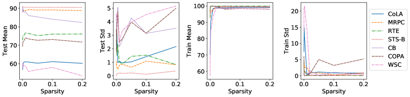
Figure 5: Effectiveness of sparsity.

	CoLA	STS-B	MRPC	RTE	CB	COPA	WSC	AVG
FullTuning	60.74[2]±1.89	90.11[3]±0.26	88.74[3]±1.08	75.37[3]±1.93	84.29±4.21	69.60±2.94	54.81±7.51	74.81±2.83
Random	56.00±1.84	89.79±0.20	88.57±0.72[2]	73.00±2.01	89.29[2]±4.92	70.30±2.69[3]	56.87±4.29	74.83±2.38
MixOut	60.37[3]±1.33	90.11[3]±0.13[3]	88.50±0.78[3]	74.51±1.28[2]	83.75±3.14[3]	69.40±4.80	57.88±6.15	74.93[3]±2.52
Bitfit	55.26±0.78[1]	89.98±0.15	86.87±1.27	71.36±1.71	91.29[1]±2.27[1]	71.80[2]±3.92	55.29±9.90	74.55±2.86
MagPruning	56.45±1.80	90.26[2]±0.11[1]	87.35±0.85	72.24±2.14	84.46±3.58	69.20±3.54	59.71[1]±3.88[2]	74.24±2.27[2]
Adapter	60.05±1.88	89.92±0.19	88.79[1]±0.80	74.55±1.80	86.61±4.97	68.80±2.40[1]	55.63±7.53	74.91±2.79
LoRA	61.46[1]±1.27[3]	86.73±0.38	88.28±1.06	76.46[1]±1.34[3]	88.69[3]±5.32	67.75±2.49[2]	58.85[3]±4.27[3]	75.46[2]±2.30[3]
DiffPruning	58.36±1.45	89.52±0.27	77.46±5.31	70.76±9.01	85.18±2.65[2]	70.40[3]±3.07	55.38±4.30	72.44±3.72
ChildPruning	59.40±2.30	89.33±3.23	88.43±0.80	75.11±2.87	85.71±4.07	70.30±4.54	54.04±7.24	74.62±3.58
SAM	59.52±1.12[2]	90.45[1]±0.12[2]	88.79[1]±0.69[1]	75.74[2]±1.27[1]	86.79±4.39	74.00[1]±2.79	59.52[2]±3.32[1]	76.40[1]±1.96[1]

Table 2: Data perturbation stability. The setting is the same as the main experiments except that we run the experiments on different sampled datasets. Due to the space limit, we attach the significance test in Appendix A.7.

Projection Discontinuity Problem. To give an intuitive illustration of the projection discontinuity problem in projection-based approaches, we plot the training curve of the DiffPruning method on the CB task. As illustrated in Fig. 4, we adjust the mask every 600 training steps. It can be observed from the figure that each time we change the mask, the training error will go back to almost the same value as its initial loss. This result shows that changing the mask severely affects the training procedure due to the projection discontinuity problem.

Relation between Stability and Overall Performance. Theorem 2 shows that stability implies better generalization. To further validate this, we illustrate how the stability ranks and the overall performance ranks are correlated in the main experiment. As shown in Fig. 4, the x-axis is the stability rank in each main experiment while the y-axis is the corresponding overall performance rank. For each vertical line of a specific stability rank, the dot indicates the overall performance mean rank value while the line length indicates the standard deviation. It can be observed from the figure that the two ranks are positively correlated indicating that stabler models usually have better generalization capability. To further show the relationship between the stability and the overall performance, we calculate Spearman’s rank correlation coefficient Spearman (1904) for the two ranks. It can be denoted as $\rho=\frac{\operatorname{cov}(R(S),R(V))}{\sigma_{R(S)}\sigma_{R(V)}}$, where $R(S)$ and $R(V)$ are the rank variables, $\operatorname{cov}(R(S),R(V))$ is the covariance of $R(S)$ and $R(V)$ while $\sigma_{R(V)}$ is the standard deviation of the rank variable $V$. We have $\rho=0.4356$ with p-value$=0.000014<0.05$ indicating that the correlation between the two rank variables is significant.

Effectiveness of Sparsity. To further verify our theoretical analysis in Theorem 1 and Theorem 2, we conduct a new experiment to show how the overall performance and the stability change as we change the sparsity. We change the sparsity of the SAM model in {0.0002, 0.0005, 0.001, 0.002, 0.005, 0.01, 0.02, 0.05, 0.1, 0.2} and plot the relationship between sparsity and the mean/standard deviation in both the test set and training set. The results are shown in Fig. 5. It can be concluded from the results that (1) as the sparsity ratio decreases, the mean and the standard deviation of most tasks also decrease which means the models become more stable with better generalization. This observation is consistent with our bound in Theorem 1 and Theorem 2. (2) If the sparsity ratio drops below a certain threshold, the models become quite unstable and the performance also sees a sharp drop. This is because the empirical error increases drastically which can be observed in the Train Mean and Train Std scores in Fig. 5. At the same time, under such circumstances, decreasing the sparsity ratio cannot further lower the bound effectively. Therefore, such observation is also consistent with our discussion in Theorem 1 and Theorem 2.

Data Perturbation Stability. In the main experiment, we use different random seeds. However, it is unknown whether the performance is still stable if we have a perturbation on the dataset. We conduct a new experiment to verify the data perturbation stability by training the model on 10 different training sets. Each of them is made by randomly removing 10% training samples from our original training set. The results are shown in Table 2. It can be observed from the results that the data perturbation stability performance is similar to the main experiment and our proposed SAM model still has the best data perturbation stability as well as the overall performance among all the models.

6 Related Works

Fine-tuning on a pre-trained model Peters et al. (2018); Devlin et al. (2019); Lan et al. (2020); Radford et al. (2018, 2019); Brown et al. (2020); Dong et al. (2019); Qiu et al. (2020); Chen et al. (2022); Liu et al. (2022) has shown to be very promising in recent years. However, fine-tuning the full model yields a large model with the same size for each task and many works indicate that fine-tuning the full model is unstable Devlin et al. (2019); Phang et al. (2018); Lee et al. (2019); Zhu et al. (2020); Dodge et al. (2020); Pruksachatkun et al. (2020); Mosbach et al. (2020); Zhang et al. (2020); Zhao et al. (2021). To solve this problem, many researchers propose the parameter-efficient methods which only fine-tune a small part of the pre-trained parameters. These methods are found to be more stable than fine-tuning the full model He et al. (2021b); Lee et al. (2019); Houlsby et al. (2019); Zaken et al. (2021); Sung et al. (2021); Liu et al. (2021). Currently, there is still no previous work providing a theoretical analysis for the stability of the parameter-efficient models.

Depending on how the parameter-efficient models choose which parameters to optimize, we categorize them into 1) random approaches (Random and MixoutLee et al. (2019)), 2) rule-based approaches (BitFit Zaken et al. (2021), MagPruning Han et al. (2015a, b); Lee et al. (2021), Adapter Houlsby et al. (2019); Pfeiffer et al. (2020); Rücklé et al. (2021); He et al. (2021b), LoRA Hu et al. (2022)), and 3) projection-based approaches (DiffPruning Mallya et al. (2018); Sanh et al. (2020); Guo et al. (2021), ChildPruning Xu et al. (2021)). We refer readers to section 2.2 for more detailed discussion about these models. Despite the promising results achieved by these models, the random and rule-based approaches do not utilize the information from task-specific data while the projection-based approaches have the projection discontinuity problem.

Apart from the parameter efficient fine-tuning methods, many other approaches Xuhong et al. (2018); Jiang et al. (2020); Hua et al. (2021) have also been proposed to regularize the parameters to enhance the generalization capability. Moreover, many research works Salman et al. (2020); Jiang et al. (2020); Li and Zhang (2021); Hua et al. (2021) propose to train model adversarially while some researchers You et al. (2019); Liang et al. (2021); Ansell et al. (2021); Chen et al. (2021) propose to utilize the lottery ticket approaches to prune the network. Besides, the prompt-tuning Liu et al. (2021); Lester et al. (2021); Li and Liang (2021) methods try to use prefix to adapt the model into new domains without changing the model parameters and the continuous prompts method Li and Liang (2021) can be categorized into the rule-based approaches. Currently, our work focuses on approaches that only fine-tune a small part of the model which is very different from these models in structure or procedure.

7 Conclusions

In this paper, we propose to understand the effectiveness of the parameter-efficient fine-tuning models. Depending on how the tunable parameters are chosen, we first categorize most of the models into three categories, namely, random approaches, rule-based approaches, and projection-based approaches. Then, we show that all models in the three categories are sparse fine-tuned models and we give a theoretical analysis of the stability and the generalization error. We further show that the random approaches and the rule-based methods do not utilize the task data information while the projection-based approaches suffer from the projection discontinuity problem. We propose a novel SAM model to alleviate both problems and we conduct extensive experiments to show the correctness of our theoretical analysis and the effectiveness of our proposed models.

Appendix. Supplementary Material

Appendix A.1 Proof of Proposition 1

Proposition 1.

Optimizing Problem (2) implies to optimizing the upper bound $\bar{L}$ of the following regularized problem:

$$L_{R}=\min_{\theta}\mathcal{L}(\theta)+\|(I-M)(\theta-\theta^{0})\|^{2}\leq\bar{L}.$$ (11)

Proof.

We write the Lagrangian of Problem (2) as:

$$\bar{L}=\min_{\theta}\max_{\lambda}\mathcal{L}(\theta)+\lambda\|(I-M)(\theta-\theta^{0})\|^{2}$$

where $\lambda$ is the Lagrangian multiplier. Therefore, Problem (2) is equivalent to solving the following problem:

$$\min_{\theta}\max_{\lambda}\mathcal{L}(\theta)+\lambda\|(I-M)(\theta-\theta^{0})\|^{2}$$

$$\geq\max_{\lambda}\min_{\theta}\mathcal{L}(\theta)+\lambda\|(I-M)(\theta-\theta^{0})\|^{2}$$

$$\geq\min_{\theta}\mathcal{L}(\theta)+\|(I-M)(\theta-\theta^{0})\|^{2}$$

∎

Appendix A.2 Proof of Theorem 1

Given training dataset $S=\{z_{1},\cdots,z_{n}\}$, $S^{i}=S\backslash z_{i}=\{z_{1},\cdots,z_{i-1},z_{i+1},\cdots,z_{n}\}$. Loss function $\mathcal{L}(\theta)=\frac{1}{n}\sum_{i=1}^{n}\ell(z_{i})$.

The following proof is derived from Shalev-Shwartz and Ben-David (2014) where the original Lemma utilizes the convex assumption which is not guaranteed in the neural network. We use the Taylor expansion instead of the convex assumption which makes it more suitable for describing the neural network models. However, the cost is that the bound will be related to a constant that is determined by the specific shape around the local minima.

Lemma 1.

Assume that the loss function $\ell$ is $\rho$ -Lipschitz. $\operatorname{\mathcal{A}}(S^{i})$ closes to $\operatorname{\mathcal{A}}(S)$. The Hessian matrix $\nabla^{2}\mathcal{L}(\operatorname{\mathcal{A}}(S))$ at $\operatorname{\mathcal{A}}(S)$ is a positive-semidefinite matrix with a singular value decomposition as $U\operatorname{diag}(\Lambda)U^{-1}$, $\Lambda=\{\Lambda_{1},\cdots,\Lambda_{m}\}$ and $\Lambda_{min}=\min\{\Lambda_{1},\cdots,\Lambda_{m}\}$. Then, the learning algorithm $\operatorname{\mathcal{A}}$ defined by

$$\operatorname{\mathcal{A}}(S)=\arg\min_{w}\frac{1}{n}\sum_{i=1}^{n}\ell(z_{i})+\lambda\|w-w_{0}\|^{2}$$

has pointwise hypothesis stability $\epsilon$ with rate $\frac{2\rho^{2}}{(\Lambda_{min}+2\lambda)n}$. It follows that:

$$\mathbb{E}_{S,i\sim U(n)}[|\ell(\operatorname{\mathcal{A}}(S^{i}),z_{i})-\ell(\operatorname{\mathcal{A}}(S),z_{i})|]\leq\frac{2\rho^{2}}{(\Lambda_{min}+2\lambda)n}$$

Proof.

We denote $f_{S}(w)=\mathcal{L}(w)+\lambda\|w-w_{0}\|^{2}$, and $\operatorname{\mathcal{A}}(S)=\arg\min_{w}f_{S}(w)$. As $\operatorname{\mathcal{A}}(S)$ minimize $f_{S}(w)$, we have $\nabla f_{S}(\operatorname{\mathcal{A}}(S))=0$. $\forall v$ close to $\operatorname{\mathcal{A}}(S)$, we have:

$$f_{S}(v)=f_{S}(\operatorname{\mathcal{A}}(S))+ [v-\operatorname{\mathcal{A}}(S)]^{T}\nabla f_{S}(\operatorname{\mathcal{A}}(S))+\frac{1}{2}[v-\operatorname{\mathcal{A}}(S)]^{T}\nabla^{2}f_{S}(\operatorname{\mathcal{A}}(S))[v-\operatorname{\mathcal{A}}(S)]$$

$$f_{S}(v)=f_{S}(\operatorname{\mathcal{A}}(S))+ \frac{1}{2}[v-\operatorname{\mathcal{A}}(S)]^{T}\nabla^{2}f_{S}(\operatorname{\mathcal{A}}(S))[v-\operatorname{\mathcal{A}}(S)]$$

$$f_{S}(v)-f_{S}(\operatorname{\mathcal{A}}(S)) =\frac{1}{2}[v-\operatorname{\mathcal{A}}(S)]^{T}\nabla^{2}f_{S}(\operatorname{\mathcal{A}}(S))[v-\operatorname{\mathcal{A}}(S)]$$

$$f_{S}(v)-f_{S}(\operatorname{\mathcal{A}}(S)) =\frac{1}{2}[v-\operatorname{\mathcal{A}}(S)]^{T}\nabla^{2}_{w=A(S)}(\mathcal{L}(w)+\lambda\|w-w_{0}\|^{2})[v-\operatorname{\mathcal{A}}(S)]$$

$$f_{S}(v)-f_{S}(\operatorname{\mathcal{A}}(S)) =\frac{1}{2}[v-\operatorname{\mathcal{A}}(S)]^{T}(\nabla^{2}\mathcal{L}(\operatorname{\mathcal{A}}(S))+2\lambda I)[v-\operatorname{\mathcal{A}}(S)]$$

$$f_{S}(v)-f_{S}(\operatorname{\mathcal{A}}(S)) =\frac{1}{2}[v-\operatorname{\mathcal{A}}(S)]^{T}(U\operatorname{diag}(\Lambda)U^{-1}+2\lambda I)[v-\operatorname{\mathcal{A}}(S)]$$

$$f_{S}(v)-f_{S}(\operatorname{\mathcal{A}}(S)) =\frac{1}{2}[v-\operatorname{\mathcal{A}}(S)]^{T}(U(\operatorname{diag}(\Lambda)+2\lambda I)U^{-1})[v-\operatorname{\mathcal{A}}(S)]$$

$$f_{S}(v)-f_{S}(\operatorname{\mathcal{A}}(S)) =\frac{1}{2}[v-\operatorname{\mathcal{A}}(S)]^{T}U(\operatorname{diag}(\Lambda+2\lambda)U^{-1}[v-\operatorname{\mathcal{A}}(S)]$$

$$f_{S}(v)-f_{S}(\operatorname{\mathcal{A}}(S)) =\frac{1}{2}[v-\operatorname{\mathcal{A}}(S)]^{T}U\operatorname{diag}(\sqrt{\Lambda_{1}+2\lambda},\cdots,\sqrt{\Lambda_{m}+2\lambda})\cdot$$

$$\ \ \ \ \ \ \operatorname{diag}(\sqrt{\Lambda_{1}+2\lambda},\cdots,\sqrt{\Lambda_{m}+2\lambda})U^{-1}[v-\operatorname{\mathcal{A}}(S)]$$

$$f_{S}(v)-f_{S}(\operatorname{\mathcal{A}}(S)) =\frac{1}{2}[v-\operatorname{\mathcal{A}}(S)]^{T}U\operatorname{diag}(\sqrt{\Lambda_{1}+2\lambda},\cdots,\sqrt{\Lambda_{m}+2\lambda})U^{-1}\cdot$$

$$\ \ \ \ \ \ U\operatorname{diag}(\sqrt{\Lambda_{1}+2\lambda},\cdots,\sqrt{\Lambda_{m}+2\lambda})U^{-1}[v-\operatorname{\mathcal{A}}(S)]$$

$$f_{S}(v)-f_{S}(\operatorname{\mathcal{A}}(S)) =\frac{1}{2}\|U\operatorname{diag}(\sqrt{\Lambda_{1}+2\lambda},\cdots,\sqrt{\Lambda_{m}+2\lambda})U^{-1}[v-\operatorname{\mathcal{A}}(S)]\|^{2}$$

$$f_{S}(v)-f_{S}(\operatorname{\mathcal{A}}(S)) \geq\frac{1}{2}(\Lambda_{min}+2\lambda)\|v-\operatorname{\mathcal{A}}(S)\|^{2}$$

Then, if $n$ is large enough, by the definition of $f_{S}(w)$. $\forall u,v$, we have:

$$f_{S}(v)-f_{S}(u) =L_{S}(v)+\lambda\|v-w_{0}\|^{2}-(L_{S}(u)+\lambda\|u-w_{0}\|^{2})$$

$$=L_{S^{i}}(v)+\lambda\|v-w_{0}\|^{2}-(L_{S^{i}}(u)+\lambda\|u-w_{0}\|^{2})+$$

$$\frac{\ell(v,z_{i})-\ell(u,z_{i})}{n}$$

Then, we choose $v=\operatorname{\mathcal{A}}(S^{i}),u=\operatorname{\mathcal{A}}(S)$. As $v$ minimizes $L_{S^{i}}(v)+\lambda\|v-w_{0}\|^{2}$, we have:

$$f_{S}(\operatorname{\mathcal{A}}(S^{i}))-f_{S}(\operatorname{\mathcal{A}}(S))\leq\frac{\ell(\operatorname{\mathcal{A}}(S^{i}),z_{i})-\ell(\operatorname{\mathcal{A}}(S),z_{i})}{n}$$

$$\frac{1}{2}(\Lambda_{min}+2\lambda)\|\operatorname{\mathcal{A}}(S^{i})-\operatorname{\mathcal{A}}(S)\|^{2}\leq\frac{\ell(\operatorname{\mathcal{A}}(S^{i}),z_{i})-\ell(\operatorname{\mathcal{A}}(S),z_{i})}{n}$$

As the loss function $\ell(\cdot,z_{i})$ is $\rho-$Lipschitz, we have:

$$|\ell(\operatorname{\mathcal{A}}(S^{i}),z_{i})-\ell(\operatorname{\mathcal{A}}(S),z_{i})|\leq\rho\|\operatorname{\mathcal{A}}(S^{i})-\operatorname{\mathcal{A}}(S)\|$$ (12)

Then, we have:

$$\frac{1}{2}(\Lambda_{min}+2\lambda)\|A(S^{i})-\operatorname{\mathcal{A}}(S)\|^{2}\leq\frac{\rho\|A(S^{i})-\operatorname{\mathcal{A}}(S)\|}{n}$$

$$\|A(S^{i})-\operatorname{\mathcal{A}}(S)\|\leq\frac{2\rho}{(\Lambda_{min}+2\lambda)n}$$

Then, plug back into Equation (12), we have:

$$|\ell(\operatorname{\mathcal{A}}(S^{(i)}),z_{i})-\ell(\operatorname{\mathcal{A}}(S),z_{i})|\leq\frac{2\rho^{2}}{(\Lambda_{min}+2\lambda)n}.$$

As this holds for any $S,i$ we immediately obtain:

$$\mathbb{E}_{S,i\sim U(n)}[|\ell(\operatorname{\mathcal{A}}(S^{(i)}),z_{i})-\ell(\operatorname{\mathcal{A}}(S),z_{i})|]\leq\frac{2\rho^{2}}{(\Lambda_{min}+2\lambda)n}.$$

∎

Theorem 1 (Stability).

If the loss function $\ell$ is $\rho-$Lipschitz, $\operatorname{\mathcal{A}}(S^{i})$ is close to $\operatorname{\mathcal{A}}(S)$, the Hessian matrix $\nabla^{2}\mathcal{L}(\operatorname{\mathcal{A}}(S))$ at $\operatorname{\mathcal{A}}(S)$ is positive-semidefinite with a singular value decomposition $U\operatorname{diag}(\Lambda)U^{-1}$, $\Lambda=\{\Lambda_{1},\cdots,\Lambda_{m}\}$ and $\Lambda_{min}=\min\{\Lambda_{1},\cdots,\Lambda_{m}\}$, then the expectation of the loss $\mathbb{E}_{M}L_{R}$ has a pointwise hypothesis stability as:

$$\mathbb{E}_{S,i\sim U(n)}[|\ell(\operatorname{\mathcal{A}}(S^{i}),z_{i})-\ell(\operatorname{\mathcal{A}}(S),z_{i})|]\leq\frac{2\rho^{2}}{(\Lambda_{min}+2(1-p))n}.$$ (13)

Proof.

$$\mathbb{E}_{M}L_{R} =\mathcal{L}(\theta)+\mathbb{E}\|(I-M)(\theta^{0}-\theta)\|^{2}$$

$$=\mathcal{L}(\theta)+\mathbb{E}\sum_{i=1}^{m}(1-M_{ii})^{2}(\theta^{0}_{i}-\theta_{i})^{2}$$

$$=\mathcal{L}(\theta)+\sum_{i=1}^{m}(\theta^{0}_{i}-\theta_{i})^{2}\mathbb{E}(1-M_{ii})^{2}$$

$$=\mathcal{L}(\theta)+\sum_{i=1}^{m}(\theta^{0}_{i}-\theta_{i})^{2}(1-p)$$

$$=\mathcal{L}(\theta)+(1-p)\|(\theta^{0}-\theta)\|^{2}$$

From Lemma 1, we have:

$$\mathbb{E}_{S,i\sim U(m)}[|\ell(\operatorname{\mathcal{A}}(S^{i}),z_{i})-\ell(\operatorname{\mathcal{A}}(S),z_{i})|]\leq\frac{2\rho^{2}}{(\Lambda_{min}+2(1-p))n}$$

∎

Appendix A.3 Proof of Theorem 2

We first give a Lemma from Theorem 11 of Bousquet and Elisseeff (2002). It has an extended version to random algorithms in Elisseeff et al. (2005).

Lemma 2.

For any learning algorithm $\operatorname{\mathcal{A}}$ with pointwise hypothesis stability $\beta$ with respect to a loss function such that $0\leq c(y,y^{\prime})\leq C$, we have with probability $1-\delta$,

$$R(\operatorname{\mathcal{A}},S)\leq\hat{R}(\operatorname{\mathcal{A}},S)+\sqrt{\frac{C^{2}+12Cn\beta}{2n\delta}},$$

where, $c(y,y^{\prime})=|y-y^{\prime}|$ is an absolute loss function.

Theorem 2 (Generalization).

We denote the generalization error as $R(\operatorname{\mathcal{A}},S)=\mathbb{E}_{z}\ell(\operatorname{\mathcal{A}}(S),z)$ and the empirical error as $\hat{R}(\operatorname{\mathcal{A}},S)=\frac{1}{n}\sum_{i=1}^{n}\ell(\operatorname{\mathcal{A}}(S),z)$. Then, for some constant $C$, we have with probability $1-\delta$,

$$R(\operatorname{\mathcal{A}},S)\leq\hat{R}(\operatorname{\mathcal{A}},S)+\sqrt{\frac{C^{2}+\frac{24C\rho^{2}}{\Lambda_{min}+2(1-p)}}{2n\delta}}.$$ (14)

Appendix A.4 Proof of Theorem 3

Theorem 3.

If $\hat{M}_{ii}=\mathds{1}(\sum_{j=1}^{m}\mathds{1}(|\frac{\nabla\operatorname{\mathcal{L}}(\theta^{0})_{i}^{2}}{h_{i}}|>|\frac{\nabla\operatorname{\mathcal{L}}(\theta^{0})_{j}^{2}}{h_{j}}|)\geq m-\lfloor mp\rfloor)$, where $\nabla\operatorname{\mathcal{L}}(\theta^{0})_{i}$ is the $i$th element of the gradient vector $\nabla\operatorname{\mathcal{L}}(\theta^{0})$, then

$$\inf_{\Delta\theta}\operatorname{\mathcal{L}}(\theta^{0}+\hat{M}\Delta\theta)\leq\inf_{\begin{subarray}{c}\Delta\theta,\|M\|_{0}=\lfloor mp\rfloor;\\ M_{ij}=0,\forall i\neq j;M_{ii}\in\{0,1\}\end{subarray}}\operatorname{\mathcal{L}}(\theta^{0}+M\Delta\theta).$$ (15)

Proof.

We denote $\mathcal{I}=\{i|\hat{M}_{ii}=1\}$, $\forall M\in\Omega=\{M|\|M\|_{0}=\lfloor mp\rfloor;M_{ij}=0,\forall i\neq j;M_{ii}\in\{0,1\}\}$ , we have

$$\inf_{\Delta\theta,M\in\Omega}\operatorname{\mathcal{L}}(\theta^{0}+M\Delta\theta) =\inf_{\Delta\theta,M\in\Omega}\operatorname{\mathcal{L}}(\theta^{0})+\nabla\operatorname{\mathcal{L}}(\theta^{0})^{\mathrm{T}}M\Delta\theta+\frac{1}{2}(M\Delta\theta)^{\mathrm{T}}HM\Delta\theta$$

$$=\inf_{\Delta\theta,M\in\Omega}\operatorname{\mathcal{L}}(\theta^{0})+\sum_{i=1}^{m}M_{ii}\nabla\operatorname{\mathcal{L}}(\theta^{0})_{i}\Delta\theta_{i}+\frac{1}{2}\sum_{i=1}^{m}M_{ii}h_{i}\Delta\theta_{i}^{2}$$

$$=\inf_{\Delta\theta,M\in\Omega}\operatorname{\mathcal{L}}(\theta^{0})+\sum_{i=1}^{m}M_{ii}(\frac{1}{2}h_{i}\Delta\theta_{i}^{2}+\nabla\operatorname{\mathcal{L}}(\theta^{0})_{i}\Delta\theta_{i})$$

$$=\inf_{M\in\Omega}\operatorname{\mathcal{L}}(\theta^{0})-\sum_{i=1}^{m}M_{ii}\frac{\nabla\operatorname{\mathcal{L}}(\theta^{0})_{i}^{2}}{2h_{i}}$$

$$\geq\operatorname{\mathcal{L}}(\theta^{0})-\sum_{i\in\mathcal{I}}\frac{\nabla\operatorname{\mathcal{L}}(\theta^{0})_{i}^{2}}{2h_{i}}\ \ \ \ \ \ \ \ \ \ \ \text{(By the definition of $\hat{M}$ and $\mathcal{I}$)}$$

$$=\operatorname{\mathcal{L}}(\theta^{0})-\sum_{i=1}^{m}\hat{M}_{ii}\frac{\nabla\operatorname{\mathcal{L}}(\theta^{0})_{i}^{2}}{2h_{i}}$$

$$=\inf_{\Delta\theta}\operatorname{\mathcal{L}}(\theta^{0}+\hat{M}\Delta\theta)$$

∎

Appendix A.5 Training Time Analysis

To further analyze the computational cost of each method, we list the training time for different models as shown in Table 3. It should be noted that as we adopt the early stop strategy, models stop training when they converge and the running step number may be different from each other. It can be concluded from the results that: (1) Adapter and LoRA model outperform the FullTuning model as they only tune only a few newly added parameters; (2) Other parameter-efficient models spend more time than the FullTuning model because in the current implementation, all of these models use a mask to determine which parameters to tune and thus cannot save the computational cost. (3) Our proposed SAM model outperforms all other models (except Adapter and LoRA) as it has a faster convergence rate. However, it still needs a mask and thus needs more time to train than the FullTuning model. It should be noted that as indicated by Guo et al. (2021); Houlsby et al. (2019), though most of the parameter-efficient models need more time to train, they actually need less storage space as they can just only store the changed parameters. This is quite useful when there are a lot of downstream tasks.

	CoLA	MRPC	STS-B	RTE	CB	COPA	WSC	AVG
FullTuning	0.74	1.04	1.90	2.63	3.18	0.66	1.55	1.67
ChildPruning	3.91	1.36	2.12	3.77	3.13	0.91	2.34	2.51
Adapter	0.89	1.24	3.43	3.51	1.16	0.41	0.47	1.59
LoRA	1.39	1.23	2.12	4.87	2.15	0.60	1.43	1.97
Bitfit	2.30	1.70	6.70	7.02	2.18	1.20	0.87	3.14
DiffPruning	0.60	1.07	6.61	5.30	2.86	1.21	1.06	2.67
Random	0.41	3.36	4.34	6.70	1.60	1.27	0.69	2.62
SAM	2.31	1.68	2.78	3.15	2.70	0.72	0.82	2.02

Table 3: Training time (in hour) analysis.

Appendix A.6 Tunable Parameter Ratio Comparison

To make the model results comparable with each other, we try our best to set the tunable parameter ratio for each experiment as close as possible. Table 4 shows the ratio of tunable parameters for each model. The tunable parameters for Adapter and BitFit are fixed and cannot be changed. We follow the official setting for the LoRA model to set the size of the tunable parameters. For other models including our proposed SAM model, we follow Guo et al. (2021) to set the tunable ratio as 0.5% to make the models comparable with each other.

	FullTuning	ChildPruning	Adapter	LoRA	Bitfit	DiffPruning	Random	MixOut	MagPruning	SAM
%Param	100	0.5	0.72	0.91	0.09	0.5	0.5	0.5	0.5	0.5

Table 4: Tunable parameter ratio comparison.

Appendix A.7 T-Test of the Significance of SAM

To show how significantly our proposed SAM model outperforms other models, we conduct a t-test by comparing the SAM’s results with other models’ results. If the SAM model outperforms another model, the t-statistics will be greater than 0. If it outperforms another model significantly, the p-value will be less than 0.05. We report the t-statistics/p-value for the main experiment in Table 5 as well as the corresponding results for the data perturbation experiments in Table 6. We can conclude from the experimental results that our proposed SAM model outperforms the corresponding model significantly with p-values ¡ 0.05. It shows that SAM model can outperform the other models in most of the cases.

	CoLA	STS-B	MRPC	RTE	CB	COPA	WSC
FullTuning	3.81/0.00	4.43/0.00	-1.69/0.11	0.83/0.42	-0.00/1.00	3.36/0.00	2.91/0.01
Random	5.38/0.00	12.34/0.00	0.60/0.56	3.35/0.00	-1.26/0.22	3.47/0.00	3.13/0.01
MixOut	3.07/0.01	5.81/0.00	0.83/0.42	-0.96/0.35	1.60/0.13	1.47/0.16	2.84/0.01
Bitfit	7.27/0.00	6.89/0.00	4.68/0.00	4.04/0.00	1.62/0.12	1.73/0.10	2.39/0.03
MagPruning	4.88/0.00	4.34/0.00	2.43/0.03	3.78/0.00	5.88/0.00	1.83/0.08	2.84/0.01
Adapter	-2.34/0.03	7.93/0.00	-1.12/0.28	-0.16/0.87	0.98/0.34	3.07/0.01	1.60/0.13
LoRA	0.02/0.99	18.99/0.00	-1.87/0.08	-0.21/0.84	3.10/0.01	2.85/0.01	1.76/0.10
DiffPruning	4.00/0.00	8.16/0.00	4.97/0.00	2.55/0.02	2.53/0.02	1.38/0.18	3.78/0.00
ChildPruning	1.67/0.11	1.27/0.22	1.35/0.19	0.66/0.52	1.90/0.07	2.63/0.02	2.59/0.02

Table 5: T-Test results (t-statistics/p-value) for comparing SAM with other models in each tasks. We use green color if the t-statistics is larger than 0 while the p-value ¡ 0.05. It shows the SAM model outperforms the corresponding model significantly. We use red color if the t-statistics is less than 0 while the p-value ¡ 0.05. It shows the corresponding model outperforms the SAM model significantly. The uncolored text means there is no statistical significance with respect to p-value=0.05.

	CoLA	STS-B	MRPC	RTE	CB	COPA	WSC
FullTuning	-0.25/0.81	3.61/0.00	0.12/0.90	1.14/0.27	1.23/0.23	3.26/0.00	1.76/0.10
Random	3.72/0.00	7.99/0.00	0.66/0.52	3.68/0.00	-1.14/0.27	2.96/0.01	2.49/0.02
MixOut	0.06/0.95	5.33/0.00	0.82/0.42	2.47/0.02	1.69/0.11	2.48/0.02	0.78/0.44
Bitfit	6.34/0.00	6.65/0.00	3.99/0.00	5.64/0.00	-2.49/0.02	1.37/0.19	1.27/0.22
MagPruning	3.39/0.01	3.22/0.00	3.96/0.00	4.34/0.00	1.23/0.23	3.19/0.01	0.05/0.96
Adapter	0.32/0.75	6.82/0.00	-0.02/0.99	2.14/0.05	0.08/0.94	6.23/0.00	2.64/0.02
LoRA	-1.09/0.30	26.73/0.00	1.21/0.24	0.00/1.00	-0.72/0.48	4.67/0.00	0.49/0.63
DiffPruning	2.04/0.06	9.16/0.00	6.34/0.00	1.85/0.08	0.94/0.36	2.60/0.02	2.24/0.04
ChildPruning	0.74/0.48	1.05/0.31	1.02/0.32	1.16/0.26	0.54/0.60	2.08/0.05	2.09/0.05

Table 6: T-Test for significance of SAM in data perturbation stability experiments. The color scheme is the same as Table 5.

Appendix A.8 Limitations and Future Directions

In this work, we theoretically prove the SAM model achieves approximal optimal value with Theorem 3 with the second-order approximation. Therefore, there is still some room for improvement for the real target function. We can consider exploring some other assumptions of the target function like quadratic growth, Polyak-Łojasiewicz, etc. We may get different approximate optimal solutions under different assumptions. Besides, though the current model achieves better results with better stability, the training time is a little bit longer than the full tuning model. This is because, in the current implementation, the sparsity is achieved with a gradient mask. As a result, the training time may be slightly longer than an ordinary model. We can explore to further improve the implementation strategy to accelerate the running speed.

Appendix A.9 Broader Impact Statement

This paper proposes a theoretical analysis of existing methods and proposes an improved method under the same task setting. It may help researchers to understand existing models better and we also propose the SAM model to improve the model performance. The task is widely studied in the NLP community and we do not conduct any experiments with any living beings. Our work also does not cause any kind of safety or security concerns. Our work also does not raise any human rights concerns or environmental concerns. Therefore, there will be no negative societal impact on our work. All the data used in this paper come from widely used datasets and we have given a detailed description and source of the datasets. As far as we know, these datasets do not have any personally identifiable information. From the previous literature, no bias cases were reported.

References

- Ansell et al. (2021) Alan Ansell, Edoardo Maria Ponti, Anna Korhonen, and Ivan Vulić. 2021. Composable sparse fine-tuning for cross-lingual transfer. arXiv preprint arXiv:2110.07560.
- Bentivogli et al. (2009) Luisa Bentivogli, Peter Clark, Ido Dagan, and Danilo Giampiccolo. 2009. The fifth pascal recognizing textual entailment challenge. In TAC.
- Bishop and Nasrabadi (2006) Christopher M Bishop and Nasser M Nasrabadi. 2006. Pattern recognition and machine learning, volume 4. Springer.
- Bollapragada et al. (2019) Raghu Bollapragada, Richard H Byrd, and Jorge Nocedal. 2019. Exact and inexact subsampled newton methods for optimization. IMA Journal of Numerical Analysis, 39(2):545–578.
- Bousquet and Elisseeff (2002) Olivier Bousquet and André Elisseeff. 2002. Stability and generalization. The Journal of Machine Learning Research, 2:499–526.
- Brown et al. (2020) Tom Brown, Benjamin Mann, Nick Ryder, Melanie Subbiah, Jared D Kaplan, Prafulla Dhariwal, Arvind Neelakantan, Pranav Shyam, Girish Sastry, Amanda Askell, et al. 2020. Language models are few-shot learners. Advances in neural information processing systems, 33:1877–1901.
- Cer et al. (2017) Daniel Cer, Mona Diab, Eneko Agirre, Inigo Lopez-Gazpio, and Lucia Specia. 2017. Semeval-2017 task 1: Semantic textual similarity-multilingual and cross-lingual focused evaluation. arXiv preprint arXiv:1708.00055.
- Charles and Papailiopoulos (2018) Zachary Charles and Dimitris Papailiopoulos. 2018. Stability and generalization of learning algorithms that converge to global optima. In International conference on machine learning, pages 745–754. PMLR.
- Chen et al. (2022) Guanzheng Chen, Fangyu Liu, Zaiqiao Meng, and Shangsong Liang. 2022. Revisiting parameter-efficient tuning: Are we really there yet? arXiv preprint arXiv:2202.07962.
- Chen et al. (2021) Xiaohan Chen, Yu Cheng, Shuohang Wang, Zhe Gan, Zhangyang Wang, and Jingjing Liu. 2021. Earlybert: Efficient bert training via early-bird lottery tickets. In Proceedings of the 59th Annual Meeting of the Association for Computational Linguistics and the 11th International Joint Conference on Natural Language Processing (Volume 1: Long Papers), pages 2195–2207.
- Dagan et al. (2005) Ido Dagan, Oren Glickman, and Bernardo Magnini. 2005. The pascal recognising textual entailment challenge. In Machine Learning Challenges Workshop, pages 177–190. Springer.
- De Marneffe et al. (2019) Marie-Catherine De Marneffe, Mandy Simons, and Judith Tonhauser. 2019. The commitmentbank: Investigating projection in naturally occurring discourse. In proceedings of Sinn und Bedeutung, volume 23, pages 107–124.
- Dembo et al. (1982) Ron S Dembo, Stanley C Eisenstat, and Trond Steihaug. 1982. Inexact newton methods. SIAM Journal on Numerical analysis, 19(2):400–408.
- Devlin et al. (2019) Jacob Devlin, Ming-Wei Chang, Kenton Lee, and Kristina Toutanova. 2019. Bert: Pre-training of deep bidirectional transformers for language understanding. In Proceedings of NAACL-HLT, pages 4171–4186.
- Ding et al. (2022) Ning Ding, Yujia Qin, Guang Yang, Fuchao Wei, Zonghan Yang, Yusheng Su, Shengding Hu, Yulin Chen, Chi-Min Chan, Weize Chen, et al. 2022. Delta tuning: A comprehensive study of parameter efficient methods for pre-trained language models. arXiv preprint arXiv:2203.06904.
- Dodge et al. (2020) Jesse Dodge, Gabriel Ilharco, Roy Schwartz, Ali Farhadi, Hannaneh Hajishirzi, and Noah A Smith. 2020. Fine-tuning pretrained language models: Weight initializations, data orders, and early stopping.
- Dolan and Brockett (2005) Bill Dolan and Chris Brockett. 2005. Automatically constructing a corpus of sentential paraphrases. In Third International Workshop on Paraphrasing (IWP2005).
- Dong et al. (2019) Li Dong, Nan Yang, Wenhui Wang, Furu Wei, Xiaodong Liu, Yu Wang, Jianfeng Gao, Ming Zhou, and Hsiao-Wuen Hon. 2019. Unified language model pre-training for natural language understanding and generation. Advances in Neural Information Processing Systems, 32.
- Elisseeff et al. (2005) Andre Elisseeff, Theodoros Evgeniou, Massimiliano Pontil, and Leslie Pack Kaelbing. 2005. Stability of randomized learning algorithms. Journal of Machine Learning Research, 6(1).
- Fedus et al. (2021) William Fedus, Barret Zoph, and Noam Shazeer. 2021. Switch transformers: Scaling to trillion parameter models with simple and efficient sparsity. arXiv preprint arXiv:2101.03961.
- Fu et al. (2021) Zihao Fu, Wai Lam, Anthony Man-Cho So, and Bei Shi. 2021. A theoretical analysis of the repetition problem in text generation. In Proceedings of the AAAI Conference on Artificial Intelligence, volume 35, pages 12848–12856.
- Giampiccolo et al. (2007) Danilo Giampiccolo, Bernardo Magnini, Ido Dagan, and William B Dolan. 2007. The third pascal recognizing textual entailment challenge. In Proceedings of the ACL-PASCAL workshop on textual entailment and paraphrasing, pages 1–9.
- Guo et al. (2021) Demi Guo, Alexander M Rush, and Yoon Kim. 2021. Parameter-efficient transfer learning with diff pruning. In Proceedings of the 59th Annual Meeting of the Association for Computational Linguistics and the 11th International Joint Conference on Natural Language Processing (Volume 1: Long Papers), pages 4884–4896.
- Han et al. (2015a) Song Han, Huizi Mao, and William J Dally. 2015a. Deep compression: Compressing deep neural networks with pruning, trained quantization and huffman coding. arXiv preprint arXiv:1510.00149.
- Han et al. (2015b) Song Han, Jeff Pool, John Tran, and William Dally. 2015b. Learning both weights and connections for efficient neural network. Advances in neural information processing systems, 28.
- Hardt et al. (2016) Moritz Hardt, Ben Recht, and Yoram Singer. 2016. Train faster, generalize better: Stability of stochastic gradient descent. In International conference on machine learning, pages 1225–1234. PMLR.
- He et al. (2021a) Junxian He, Chunting Zhou, Xuezhe Ma, Taylor Berg-Kirkpatrick, and Graham Neubig. 2021a. Towards a unified view of parameter-efficient transfer learning. arXiv preprint arXiv:2110.04366.
- He et al. (2021b) Ruidan He, Linlin Liu, Hai Ye, Qingyu Tan, Bosheng Ding, Liying Cheng, Jiawei Low, Lidong Bing, and Luo Si. 2021b. On the effectiveness of adapter-based tuning for pretrained language model adaptation. In Proceedings of the 59th Annual Meeting of the Association for Computational Linguistics and the 11th International Joint Conference on Natural Language Processing (Volume 1: Long Papers), pages 2208–2222.
- Houlsby et al. (2019) Neil Houlsby, Andrei Giurgiu, Stanislaw Jastrzebski, Bruna Morrone, Quentin De Laroussilhe, Andrea Gesmundo, Mona Attariyan, and Sylvain Gelly. 2019. Parameter-efficient transfer learning for nlp. In International Conference on Machine Learning, pages 2790–2799. PMLR.
- Hu et al. (2022) Edward J Hu, yelong shen, Phillip Wallis, Zeyuan Allen-Zhu, Yuanzhi Li, Shean Wang, Lu Wang, and Weizhu Chen. 2022. LoRA: Low-rank adaptation of large language models. In International Conference on Learning Representations.
- Hua et al. (2021) Hang Hua, Xingjian Li, Dejing Dou, Chengzhong Xu, and Jiebo Luo. 2021. Noise stability regularization for improving bert fine-tuning. In Proceedings of the 2021 Conference of the North American Chapter of the Association for Computational Linguistics: Human Language Technologies, pages 3229–3241.
- Jiang et al. (2020) Haoming Jiang, Pengcheng He, Weizhu Chen, Xiaodong Liu, Jianfeng Gao, and Tuo Zhao. 2020. Smart: Robust and efficient fine-tuning for pre-trained natural language models through principled regularized optimization. In Proceedings of the 58th Annual Meeting of the Association for Computational Linguistics, pages 2177–2190.
- Karimi Mahabadi et al. (2021) Rabeeh Karimi Mahabadi, James Henderson, and Sebastian Ruder. 2021. Compacter: Efficient low-rank hypercomplex adapter layers. Advances in Neural Information Processing Systems, 34.
- Kenton and Toutanova (2019) Jacob Devlin Ming-Wei Chang Kenton and Lee Kristina Toutanova. 2019. Bert: Pre-training of deep bidirectional transformers for language understanding. In Proceedings of NAACL-HLT, pages 4171–4186.
- Kim et al. (2021) Seungwon Kim, Alex Shum, Nathan Susanj, and Jonathan Hilgart. 2021. Revisiting pretraining with adapters. In Proceedings of the 6th Workshop on Representation Learning for NLP (RepL4NLP-2021), pages 90–99.
- Kuzborskij and Lampert (2018) Ilja Kuzborskij and Christoph Lampert. 2018. Data-dependent stability of stochastic gradient descent. In International Conference on Machine Learning, pages 2815–2824. PMLR.
- Lagunas et al. (2021) François Lagunas, Ella Charlaix, Victor Sanh, and Alexander M Rush. 2021. Block pruning for faster transformers. In Proceedings of the 2021 Conference on Empirical Methods in Natural Language Processing, pages 10619–10629.
- Lan et al. (2020) Zhenzhong Lan, Mingda Chen, Sebastian Goodman, Kevin Gimpel, Piyush Sharma, and Radu Soricut. 2020. Albert: A lite bert for self-supervised learning of language representations. In International Conference on Learning Representations.
- Lee et al. (2019) Cheolhyoung Lee, Kyunghyun Cho, and Wanmo Kang. 2019. Mixout: Effective regularization to finetune large-scale pretrained language models. In International Conference on Learning Representations.
- Lee et al. (2021) Jaeho Lee, Sejun Park, Sangwoo Mo, Sungsoo Ahn, and Jinwoo Shin. 2021. Layer-adaptive sparsity for the magnitude-based pruning. In International Conference on Learning Representations.
- Lester et al. (2021) Brian Lester, Rami Al-Rfou, and Noah Constant. 2021. The power of scale for parameter-efficient prompt tuning. In Proceedings of the 2021 Conference on Empirical Methods in Natural Language Processing, pages 3045–3059.
- Levesque et al. (2012) Hector Levesque, Ernest Davis, and Leora Morgenstern. 2012. The winograd schema challenge. In Thirteenth international conference on the principles of knowledge representation and reasoning.
- Lewis et al. (2020) Mike Lewis, Yinhan Liu, Naman Goyal, Marjan Ghazvininejad, Abdelrahman Mohamed, Omer Levy, Veselin Stoyanov, and Luke Zettlemoyer. 2020. Bart: Denoising sequence-to-sequence pre-training for natural language generation, translation, and comprehension. In Proceedings of the 58th Annual Meeting of the Association for Computational Linguistics, pages 7871–7880.
- Li and Zhang (2021) Dongyue Li and Hongyang Zhang. 2021. Improved regularization and robustness for fine-tuning in neural networks. Advances in Neural Information Processing Systems, 34.
- Li and Liang (2021) Xiang Lisa Li and Percy Liang. 2021. Prefix-tuning: Optimizing continuous prompts for generation. In Proceedings of the 59th Annual Meeting of the Association for Computational Linguistics and the 11th International Joint Conference on Natural Language Processing (Volume 1: Long Papers), pages 4582–4597.
- Liang et al. (2021) Jianze Liang, Chengqi Zhao, Mingxuan Wang, Xipeng Qiu, and Lei Li. 2021. Finding sparse structures for domain specific neural machine translation. In Proceedings of the AAAI Conference on Artificial Intelligence, volume 35, pages 13333–13342.
- Liu et al. (2022) Haokun Liu, Derek Tam, Mohammed Muqeeth, Jay Mohta, Tenghao Huang, Mohit Bansal, and Colin Raffel. 2022. Few-shot parameter-efficient fine-tuning is better and cheaper than in-context learning.
- Liu et al. (2021) Xiao Liu, Kaixuan Ji, Yicheng Fu, Zhengxiao Du, Zhilin Yang, and Jie Tang. 2021. P-tuning v2: Prompt tuning can be comparable to fine-tuning universally across scales and tasks. arXiv preprint arXiv:2110.07602.
- Liu et al. (2019) Yinhan Liu, Myle Ott, Naman Goyal, Jingfei Du, Mandar Joshi, Danqi Chen, Omer Levy, Mike Lewis, Luke Zettlemoyer, and Veselin Stoyanov. 2019. Roberta: A robustly optimized bert pretraining approach.
- Mahabadi et al. (2021) Rabeeh Karimi Mahabadi, Sebastian Ruder, Mostafa Dehghani, and James Henderson. 2021. Parameter-efficient multi-task fine-tuning for transformers via shared hypernetworks. In Proceedings of the 59th Annual Meeting of the Association for Computational Linguistics and the 11th International Joint Conference on Natural Language Processing (Volume 1: Long Papers), pages 565–576.
- Mallya et al. (2018) Arun Mallya, Dillon Davis, and Svetlana Lazebnik. 2018. Piggyback: Adapting a single network to multiple tasks by learning to mask weights. In Proceedings of the European Conference on Computer Vision (ECCV), pages 67–82.
- Mao et al. (2021) Yuning Mao, Lambert Mathias, Rui Hou, Amjad Almahairi, Hao Ma, Jiawei Han, Wen-tau Yih, and Madian Khabsa. 2021. Unipelt: A unified framework for parameter-efficient language model tuning. arXiv preprint arXiv:2110.07577.
- Mosbach et al. (2020) Marius Mosbach, Maksym Andriushchenko, and Dietrich Klakow. 2020. On the stability of fine-tuning bert: Misconceptions, explanations, and strong baselines. In International Conference on Learning Representations.
- Mostafa and Wang (2019) Hesham Mostafa and Xin Wang. 2019. Parameter efficient training of deep convolutional neural networks by dynamic sparse reparameterization. In International Conference on Machine Learning, pages 4646–4655. PMLR.
- Panahi et al. (2021) Aliakbar Panahi, Seyran Saeedi, and Tom Arodz. 2021. Shapeshifter: a parameter-efficient transformer using factorized reshaped matrices. Advances in Neural Information Processing Systems, 34.
- Peters et al. (2018) Matthew E. Peters, Mark Neumann, Mohit Iyyer, Matt Gardner, Christopher Clark, Kenton Lee, and Luke Zettlemoyer. 2018. Deep contextualized word representations. In NAACL.
- Pfeiffer et al. (2020) Jonas Pfeiffer, Andreas Rücklé, Clifton Poth, Aishwarya Kamath, Ivan Vulić, Sebastian Ruder, Kyunghyun Cho, and Iryna Gurevych. 2020. Adapterhub: A framework for adapting transformers. In Proceedings of the 2020 Conference on Empirical Methods in Natural Language Processing: System Demonstrations, pages 46–54.
- Phang et al. (2018) Jason Phang, Thibault Févry, and Samuel R Bowman. 2018. Sentence encoders on stilts: Supplementary training on intermediate labeled-data tasks.
- Phang et al. (2020) Jason Phang, Phil Yeres, Jesse Swanson, Haokun Liu, Ian F. Tenney, Phu Mon Htut, Clara Vania, Alex Wang, and Samuel R. Bowman. 2020. jiant 2.0: A software toolkit for research on general-purpose text understanding models. http://jiant.info/.
- Pruksachatkun et al. (2020) Yada Pruksachatkun, Jason Phang, Haokun Liu, Phu Mon Htut, Xiaoyi Zhang, Richard Yuanzhe Pang, Clara Vania, Katharina Kann, and Samuel Bowman. 2020. Intermediate-task transfer learning with pretrained language models: When and why does it work? In Proceedings of the 58th Annual Meeting of the Association for Computational Linguistics, pages 5231–5247.
- Qiu et al. (2020) Xipeng Qiu, Tianxiang Sun, Yige Xu, Yunfan Shao, Ning Dai, and Xuanjing Huang. 2020. Pre-trained models for natural language processing: A survey. Science China Technological Sciences, 63(10):1872–1897.
- Radford et al. (2018) Alec Radford, Karthik Narasimhan, Tim Salimans, and Ilya Sutskever. 2018. Improving language understanding by generative pre-training.
- Radford et al. (2019) Alec Radford, Jeffrey Wu, Rewon Child, David Luan, Dario Amodei, Ilya Sutskever, et al. 2019. Language models are unsupervised multitask learners. OpenAI blog, 1(8):9.
- Radiya-Dixit and Wang (2020) Evani Radiya-Dixit and Xin Wang. 2020. How fine can fine-tuning be? learning efficient language models. In International Conference on Artificial Intelligence and Statistics, pages 2435–2443. PMLR.
- Raffel et al. (2020) Colin Raffel, Noam Shazeer, Adam Roberts, Katherine Lee, Sharan Narang, Michael Matena, Yanqi Zhou, Wei Li, and Peter J Liu. 2020. Exploring the limits of transfer learning with a unified text-to-text transformer. Journal of Machine Learning Research, 21:1–67.
- Ricotti et al. (1988) Lucio Prina Ricotti, Susanna Ragazzini, and Giuseppe Martinelli. 1988. Learning of word stress in a sub-optimal second order back-propagation neural network. In ICNN, volume 1, pages 355–361.
- Roemmele et al. (2011) Melissa Roemmele, Cosmin Adrian Bejan, and Andrew S Gordon. 2011. Choice of plausible alternatives: An evaluation of commonsense causal reasoning. In AAAI spring symposium: logical formalizations of commonsense reasoning, pages 90–95.
- Rücklé et al. (2021) Andreas Rücklé, Gregor Geigle, Max Glockner, Tilman Beck, Jonas Pfeiffer, Nils Reimers, and Iryna Gurevych. 2021. Adapterdrop: On the efficiency of adapters in transformers. In Proceedings of the 2021 Conference on Empirical Methods in Natural Language Processing, pages 7930–7946.
- Salman et al. (2020) Hadi Salman, Andrew Ilyas, Logan Engstrom, Ashish Kapoor, and Aleksander Madry. 2020. Do adversarially robust imagenet models transfer better? Advances in Neural Information Processing Systems, 33:3533–3545.
- Sanh et al. (2020) Victor Sanh, Thomas Wolf, and Alexander Rush. 2020. Movement pruning: Adaptive sparsity by fine-tuning. Advances in Neural Information Processing Systems, 33:20378–20389.
- Shalev-Shwartz and Ben-David (2014) Shai Shalev-Shwartz and Shai Ben-David. 2014. Understanding machine learning: From theory to algorithms. Cambridge university press.
- Shalev-Shwartz et al. (2010) Shai Shalev-Shwartz, Ohad Shamir, Nathan Srebro, and Karthik Sridharan. 2010. Learnability, stability and uniform convergence. The Journal of Machine Learning Research, 11:2635–2670.
- Spearman (1904) Charles Spearman. 1904. The proof and measurement of association between two things. The American journal of psychology, 15(1):72–101.
- Sung et al. (2021) Yi-Lin Sung, Varun Nair, and Colin A Raffel. 2021. Training neural networks with fixed sparse masks. Advances in Neural Information Processing Systems, 34.
- Wang et al. (2019) Alex Wang, Yada Pruksachatkun, Nikita Nangia, Amanpreet Singh, Julian Michael, Felix Hill, Omer Levy, and Samuel Bowman. 2019. Superglue: A stickier benchmark for general-purpose language understanding systems. Advances in neural information processing systems, 32.
- Wang et al. (2018) Alex Wang, Amanpreet Singh, Julian Michael, Felix Hill, Omer Levy, and Samuel Bowman. 2018. Glue: A multi-task benchmark and analysis platform for natural language understanding. In Proceedings of the 2018 EMNLP Workshop BlackboxNLP: Analyzing and Interpreting Neural Networks for NLP, pages 353–355.
- Warstadt et al. (2019) Alex Warstadt, Amanpreet Singh, and Samuel R Bowman. 2019. Neural network acceptability judgments. Transactions of the Association for Computational Linguistics, 7:625–641.
- Wolf et al. (2020) Thomas Wolf, Lysandre Debut, Victor Sanh, Julien Chaumond, Clement Delangue, Anthony Moi, Pierric Cistac, Tim Rault, Rémi Louf, Morgan Funtowicz, Joe Davison, Sam Shleifer, Patrick von Platen, Clara Ma, Yacine Jernite, Julien Plu, Canwen Xu, Teven Le Scao, Sylvain Gugger, Mariama Drame, Quentin Lhoest, and Alexander M. Rush. 2020. Transformers: State-of-the-art natural language processing. In Proceedings of the 2020 Conference on Empirical Methods in Natural Language Processing: System Demonstrations, pages 38–45, Online. Association for Computational Linguistics.
- Xu et al. (2020) Peng Xu, Fred Roosta, and Michael W Mahoney. 2020. Newton-type methods for non-convex optimization under inexact hessian information. Mathematical Programming, 184(1):35–70.
- Xu et al. (2021) Runxin Xu, Fuli Luo, Zhiyuan Zhang, Chuanqi Tan, Baobao Chang, Songfang Huang, and Fei Huang. 2021. Raise a child in large language model: Towards effective and generalizable fine-tuning. In Proceedings of the 2021 Conference on Empirical Methods in Natural Language Processing, pages 9514–9528.
- Xuhong et al. (2018) LI Xuhong, Yves Grandvalet, and Franck Davoine. 2018. Explicit inductive bias for transfer learning with convolutional networks. In International Conference on Machine Learning, pages 2825–2834. PMLR.
- Yao et al. (2021a) Zhewei Yao, Amir Gholami, Sheng Shen, Mustafa Mustafa, Kurt Keutzer, and Michael Mahoney. 2021a. Adahessian: An adaptive second order optimizer for machine learning. In Proceedings of the AAAI Conference on Artificial Intelligence, volume 35, pages 10665–10673.
- Yao et al. (2021b) Zhewei Yao, Peng Xu, Fred Roosta, and Michael W Mahoney. 2021b. Inexact nonconvex newton-type methods. Informs Journal on Optimization, 3(2):154–182.
- You et al. (2019) Haoran You, Chaojian Li, Pengfei Xu, Yonggan Fu, Yue Wang, Xiaohan Chen, Richard G Baraniuk, Zhangyang Wang, and Yingyan Lin. 2019. Drawing early-bird tickets: Toward more efficient training of deep networks. In International Conference on Learning Representations.
- Zaken et al. (2021) Elad Ben Zaken, Shauli Ravfogel, and Yoav Goldberg. 2021. Bitfit: Simple parameter-efficient fine-tuning for transformer-based masked language-models. arXiv preprint arXiv:2106.10199.
- Zhang et al. (2020) Tianyi Zhang, Felix Wu, Arzoo Katiyar, Kilian Q Weinberger, and Yoav Artzi. 2020. Revisiting few-sample bert fine-tuning. In International Conference on Learning Representations.
- Zhao et al. (2021) Zihao Zhao, Eric Wallace, Shi Feng, Dan Klein, and Sameer Singh. 2021. Calibrate before use: Improving few-shot performance of language models. In International Conference on Machine Learning, pages 12697–12706. PMLR.
- Zhu et al. (2020) Chen Zhu, Yu Cheng, Zhe Gan, Siqi Sun, Tom Goldstein, and Jingjing Liu. 2020. Freelb: Enhanced adversarial training for natural language understanding. In ICLR.