Patterns in transitional shear turbulence.
Part 2: Emergence and optimal wavelength

Abstract

Low Reynolds number turbulence in wall-bounded shear flows en route to laminar flow takes the form of oblique, spatially-intermittent turbulent structures. In plane Couette flow, these emerge from uniform turbulence via a spatiotemporal intermittent process in which localised quasi-laminar gaps randomly nucleate and disappear. For slightly lower Reynolds numbers, spatially periodic and approximately stationary turbulent-laminar patterns predominate. The statistics of quasi-laminar regions, including the distributions of space and time scales and their Reynolds number dependence, are analysed. A smooth, but marked transition is observed between uniform turbulence and flow with intermittent quasi-laminar gaps, whereas the transition from gaps to regular patterns is more gradual. Wavelength selection in these patterns is analysed via numerical simulations in oblique domains of various sizes. Via lifetime measurements in minimal domains, and a wavelet-based analysis of wavelength predominance in a large domain, we quantify the existence and non-linear stability of a pattern as a function of wavelength and Reynolds number. We report that the preferred wavelength maximises the energy and dissipation of the large-scale flow along laminar-turbulent interfaces. This optimal behaviour is primarily due to the advective nature of the large-scale flow, with turbulent fluctuations playing only a secondary role.

1 Introduction

Turbulence in wall-bounded shear flows in the transitional regime is characterised by coexisting turbulent and laminar regions, with the turbulent fraction increasing with Reynolds number. This phenomenon was first described by Coles & van Atta (1966) and by Andereck et al. (1986) in Taylor-Couette flow. Later, by constructing Taylor-Couette and plane Couette experiments with very large aspect ratios, Prigent et al. (2002, 2003) showed that these coexisting turbulent and laminar regions, called bands and gaps respectively, spontaneously formed regular patterns with a selected wavelength and orientation that depend systematically on $Re$. These patterns have been simulated numerically and studied intensively in plane Couette flow (Barkley & Tuckerman, 2005, 2007; Duguet et al., 2010; Rolland & Manneville, 2011; Tuckerman & Barkley, 2011), plane Poiseuille flow (Tsukahara et al., 2005; Tuckerman et al., 2014; Shimizu & Manneville, 2019; Kashyap, 2021), and Taylor-Couette flow (Meseguer et al., 2009; Dong, 2009; Wang et al., 2022).

In pipe flow, the other canonical wall-bounded shear flow, only the streamwise direction is long, and transitional turbulence takes the form of puffs, also called flashes (Reynolds, 1883; Wygnanski & Champagne, 1973), which are the one-dimensional analog of turbulent bands. In contrast to bands in planar shear flows, experiments and direct numerical simulations show that puffs do not spontaneously form spatially periodic patterns (Moxey & Barkley, 2010; Avila & Hof, 2013). Instead, the spacing between them is dictated by short-range interactions (Hof et al., 2010; Samanta et al., 2011). Puffs have been extensively studied, especially in the context of the model derived by Barkley (2011a, b, 2016) from the viewpoint of excitable media. In this framework, fluctuations from uniform turbulence trigger quasi-laminar gaps (i.e. low-turbulent-energy holes within the flow) at random instants and locations, as has been seen in direct numerical simulations (DNS) of pipe flow. The bifurcation scenario giving rise to localised gaps has been investigated by Frishman & Grafke (2022), who called them anti-puffs. Interestingly, spatially periodic solutions like those observed in planar shear flows are produced in a centro-symmetric version of the Barkley model (Barkley, 2011b) although the mechanism for their formation has not yet been clarified.

In this paper, we will show that in plane Couette flow, as in pipe flow, short-lived localised gaps emerge randomly from uniform turbulence at the highest Reynolds numbers in the transitional range, which we will see is $Re\simeq 470$ in the domain which we will study. The first purpose of this paper is to investigate these gaps. The emblematic regular oblique large-scale bands appear at slightly lower Reynolds numbers, which we will see is $Re\simeq 430$.

If the localised gaps are disregarded, it is natural to associate the bands with a pattern-forming instability of the uniform turbulent flow. This was first suggested by Prigent et al. (2003) and later investigated by Rolland & Manneville (2011). Manneville (2012) and Kashyap (2021) proposed a Turing mechanism to account for the appearance of patterns by constructing a reaction-diffusion model based on an extension of the Waleffe (1997) model of the streak-roll self-sustaining process. Reetz et al. (2019) discovered a sequence of bifurcations leading to a large-scale steady state that resembles a skeleton for the banded pattern, arising from tiled copies of the exact Nagata (1990) solutions of plane Couette flow. The relationship between these pattern-forming frameworks and local nucleation of gaps is unclear.

The adaptation of classic stability concepts to turbulent flows is currently a major research topic. At the simplest level, it is always formally possible to carry out linear stability analysis of a mean flow, as was done by Barkley (2006) for a limit cycle in the cylinder wake. The mean flow of uniformly turbulent plane Couette flow has been found to be linearly stable (Tuckerman et al., 2010). However, this procedure makes the drastic simplification of neglecting the Reynolds stress entirely in the stability problem and hence its interpretation is uncertain (e.g., Bengana & Tuckerman, 2021). The next level of complexity and accuracy is to represent the Reynolds stress via a closure model. However, classic closure models for homogeneous turbulence (e.g. $(K,\Omega)$) have yielded predictions that are completely incompatible with results from full numerical simulation or experiment (Tuckerman et al., 2010). Another turbulent configuration in which large, spatially periodic scales emerge are zonal jets, characteristic of geophysical turbulence. For zonal jets, a closure model provided by a cumulant expansion (Srinivasan & Young, 2012; Tobias & Marston, 2013) has led to a plausible stability analysis (Parker & Krommes, 2013). Other strategies are possible for turbulent flows in general: Kashyap et al. (2022) examined the averaged time-dependent response of uniform turbulence to large-wavelength perturbations and provided evidence for a linear instability in plane channel flow. They computed a dispersion relation which is in good agreement with the natural spacing and angle of patterns.

Classic analyses for non-turbulent pattern-forming flows, such as Rayleigh-Bénard convection or Taylor-Couette flow, yield not only a threshold and a preferred wavelength, but also existence and stability ranges for other wavelengths through the Eckhaus instability (Busse, 1981; Ahlers et al., 1986; Riecke & Paap, 1986; Tuckerman & Barkley, 1990; Cross & Greenside, 2009). As the control parameter is varied, this instability causes spatially periodic states to make transitions to other periodic states whose wavelength is preferred. Eckhaus instability is also invoked in turbulent zonal jets (Parker & Krommes, 2013). The second goal of this paper is to study the regular patterns of transitional plane Couette flow and to determine the wavelengths at which they can exist and thrive. At low enough Reynolds numbers, patterns will be shown to destabilise and to acquire a different wavelength.

Pattern formation is sometimes associated with maximisation principles obeyed by the preferred wavelength, as in the canonical Rayleigh-Bénard convection. Such principles, like maximal dissipation, also have a long history for turbulent solutions. Malkus (1954) and Busse (1981) proposed a principle of maximal heat transport, or equivalently maximal dissipation, obeyed by convective turbulent states. The maximal dissipation principle, as formulated by Malkus (1956) in shear flows, occurs in other systems such as von Kármán flow (Ozawa et al., 2001; Mihelich et al., 2017). (This principle has been somewhat controversial and was challenged by Reynolds & Tiederman (1967) within the context of stability theory. See a modern revisit of Malkus stability theory with statistical closures by Markeviciute & Kerswell (2022).) Using the energy analysis formulated in our companion paper Gomé et al. (2023), we will associate the selected wavelength to a maximal dissipation observed for the large-scale flow along the bands.

2 Numerical setup

Plane Couette flow consists of two parallel rigid plates moving at different velocities, here equal and opposite velocities $\pm U_{\text{wall}}$. Lengths are nondimensionalised by the half-gap $h$ between the plates and velocities by $U_{\text{wall}}$. The Reynolds number is defined to be $Re\equiv U_{\text{wall}}h/\nu$. We will require one further dimensional quantity that appears in the friction coefficient – the mean horizontal shear at the walls, which we denote by $U^{\prime}_{\text{wall}}$. We will use non-dimensional variables throughout except when specified. We simulate the incompressible Navier-Stokes equations

$$\frac{\partial\bm{u}}{\partial t}+\left(\bm{u}\cdot\nabla\right)\bm{u} =-\nabla p+\frac{1}{Re}\nabla^{2}\bm{u},$$ (1a)

$$\nabla\cdot\bm{u} =0,$$ (1b)

using the pseudo-spectral parallel code Channelflow (Gibson et al., 2019). Since the bands are found to be oriented obliquely with respect to the streamwise direction, we use a doubly periodic numerical domain which is tilted with respect to the streamwise direction of the flow, shown as the oblique rectangle in figure 1. This choice was introduced by Barkley & Tuckerman (2005) and has become common in studying turbulent bands (Shi et al., 2013; Lemoult et al., 2016; Paranjape et al., 2020; Tuckerman et al., 2020). The $x$ direction is chosen to be aligned with a typical turbulent band and the $z$ coordinate to be orthogonal to the band. The relationship between streamwise-spanwise coordinates and tilted band-oriented coordinates is:

$$\mathbf{e}_{\text{strm}} =\quad\cos{\theta}\,\mathbf{e}_{x}+\sin{\theta}\,\mathbf{e}_{z}$$ (2a)

$$\mathbf{e}_{\text{span}} =-\sin{\theta}\,\mathbf{e}_{x}+\cos{\theta}\,\mathbf{e}_{z}\quad$$ (2b)

The usual wall-normal coordinate is denoted by $y$ and the corresponding velocity by $v$. Thus the boundary conditions are $\bm{u}(y=\pm 1)=\pm\mathbf{e}_{\text{strm}}$ in $y$ and periodic in $x$ and $z$, together with a zero-flux constraint on the flow in the $x$ and $z$ directions. The field visualised in figure 1 comes from an additional simulation we carried out in a domain of size ($L_{\text{strm}},L_{y},L_{\text{span}})=(200,2,100)$ aligned with the streamwise-spanwise directions. Exploiting the periodic boundary conditions of the simulation, the visualisation shows four copies of the instantaneous field.

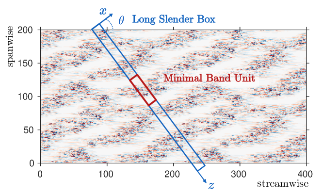
Figure 1: Spatial visualization of our numerical domains at $Re=360$. Colors show the wall-normal velocity $v$ at the midplane $y=0$ (blue: $-0.2$, white: 0, red: 0.2) in a domain of size $L_{\text{strm}}=400$, $L_{\text{span}}=200$. Red and blue boxes respectively show a Minimal Band Unit and a Long Slender Box.

The tilted box effectively reduces the dimensionality of the system by disallowing large-scale variation along the short $x$ direction. The flow in this direction is considered to be statistically homogeneous as it is only dictated by small turbulent scales. In a large non-tilted domain, bands with opposite orientations coexist (Prigent et al., 2003; Duguet et al., 2010; Klotz et al., 2022), but only one orientation is permitted in the tilted box.

We will use two types of numerical domains, with different lengths $L_{z}$. Both have fixed resolution $\Delta z=L_{z}/N_{z}=0.08$, along with fixed $L_{x}=10$ ($N_{x}=120$), $L_{y}=2$ $(N_{y}=33)$ and $\theta=24^{\circ}$. These domains are shown in figure 1.

1. Minimal Band Units, an example of which is shown as the dark red box in figure 1. These domains accommodate a single band-gap pair and so are used to study strictly periodic pattern of imposed wavelength $\lambda=L_{z}$. ($L_{z}$ must typically be below $\simeq 65$ to contain a unique band.)

2. Long Slender Boxes, which have a large $L_{z}$ direction that can accommodate a large and variable number of gaps and bands in the system. The blue box in figure 1 is an example of such a domain size with $L_{z}=240$, but larger sizes ($L_{z}=400$ or $L_{z}=800$) will be used in our study.

3 Nucleation of laminar gaps and pattern emergence

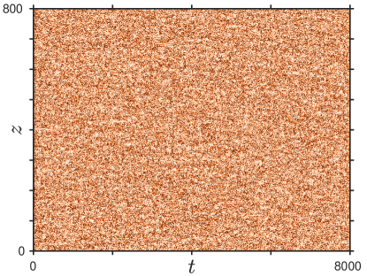
(a)

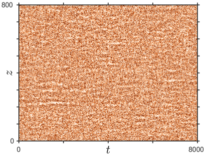
(b)

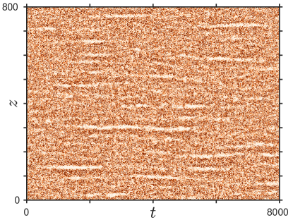
(c)

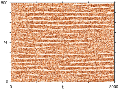
(d)

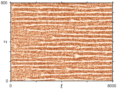
(e)

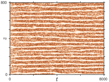
(f)

Figure 2: Spatio-temporal visualization of pattern formation with $L_{z}=800$, for (a) $Re=500$, (b) $Re=460$, (c) $440$, (d) $420$, (e) $400$ and (f) $Re=380$. Flow at $t=0$ is initiated from uniform turbulence at $Re=500$. Color shows cross-flow energy $(v^{2}+u_{\text{span}}^{2})/2$ at $x=L_{x}/2$, $y=0$ (white: 0, red: 0.02). At high $Re$, weak local gaps appear sparsely. When $Re$ is decreased, spatio-temporally intermittent patterns of finite spatial extent emerge. These consist of turbulent cores (dark red) and quasi-laminar gaps (white). For still lower $Re$, quasi-laminar regions live longer, and patterns are more regular and steady.

We have carried out simulations in a Long Slender Box of size $L_{z}=800$ for various $Re$ with the uniform turbulent state from a simulation at $Re=500$ as an initial condition, a protocol called a quench. Figure 2, an extension of figure 1 of Gomé et al. (2023, Part 1), displays the resulting spatio-temporal dynamics at six Reynolds numbers. Plotted is the $(z,t)$ dependence of the cross-flow energy $(v^{2}+u_{\text{span}}^{2})/2$ at $(x=L_{x}/2,y=0)$. The cross-flow energy is a useful diagnostic because it is zero for laminar flow and is therefore a proxy for turbulent kinetic energy. The choice $x=L_{x}/2$ is arbitrary since there is no large-scale variation of the flow field in the short $x$ direction of the simulation.

Figure 2 encapsulates the main message of this section: the emergence of patterns out of uniform turbulence is a gradual process involving spatio-temporal intermittency of turbulent and quasi-laminar flow. At $Re=500$, barely discernible low-turbulent-energy regions appear randomly within the turbulent background. At $Re=460$ these regions are more pronounced and begin to constitute localised, short-lived quasi-laminar gaps within the turbulent flow. As $Re$ is further decreased, these gaps are more probable and last for longer times. Eventually, the gaps self-organise into persistent, albeit fluctuating, patterns. The remainder of the section will quantify the evolution of states seen in figure 2.

3.1 Statistics of laminar and turbulent zones

We consider the $x,y$-averaged cross-flow energy

$$e(z,t)\equiv\frac{1}{L_{x}L_{y}}\int_{-1}^{1}\int_{0}^{L_{x}}\frac{1}{2}(v^{2}+u_{\text{span}}^{2})(x,y,z,t)~{}\mathrm{d}x\,\mathrm{d}y$$ (3)

as a useful diagnostic of quasi-laminar and turbulent zones. The probability density functions (PDFs) of $e(z,t)$ are shown in figure 3a for various values of $Re$. The right tails, corresponding to high-energy events, are broad and exponential for all $Re$. The left, low-energy portions of the PDFs vary qualitatively with $Re$, unsurprisingly since these portions correspond to the weak turbulent events and hence include the gaps. For large $Re$, the PDFs are maximal around $e\simeq 0.007$. As $Re$ is decreased, a low-energy peak emerges at $e\simeq 0.002$, corresponding to the emergence of long-lived quasi-laminar gaps seen in figure 2. The peak at $e\simeq 0.007$ flattens and gradually disappears. An interesting feature is that the distributions broaden with decreasing $Re$ with both low-energy and high-energy events becoming more likely. This reflects a spatial redistribution of energy that accompanies the formation of gaps, with turbulent bands extracting energy from quasi-laminar regions and consequently becoming more intense. (See figure 6 of Gomé et al. (2023, Part 1).)

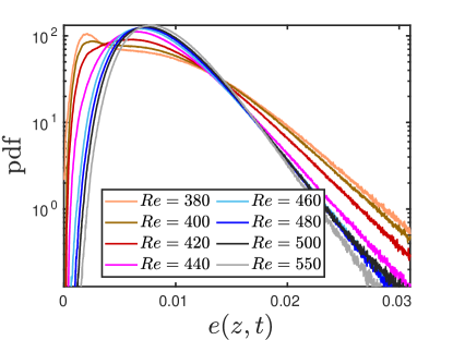
(a)

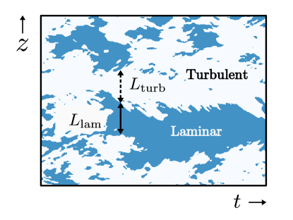
(b)

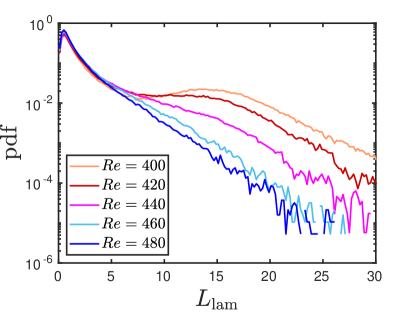
(c)

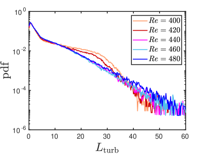
(d)

Figure 3: (a) PDFs of local cross-flow energy $e(z,t)$ defined in (3). Maximum at $e\simeq 0.002$ appears for $Re\leq 420$. (b) Illustration of the thresholding $e(z,t)<e_{\rm turb}$, of a turbulent-laminar field at $Re=440$ with turbulent regions, $e(z,t)>e_{\rm turb}$ in white and quasi-laminar regions in blue. Definitions of $L_{\rm lam}$ and $L_{\rm turb}$, the lengths of quasi-laminar and turbulent regions, are illustrated. (c) PDFs of laminar gap widths $L_{\rm lam}$ showing plateaux near 15 appearing for $Re\leq 440$. (d) PDFs of widths of turbulent regions $L_{\rm turb}$ showing local increase near 20 for $Re\leq 420$.

An intuitive way to define turbulent and quasi-laminar regions is by thresholding the values of $e(z,t)$. In the following, a region will be called quasi-laminar if $e(z,t)<e_{\rm turb}$ and turbulent if $e(z,t)\geq e_{\rm turb}$. As the PDF of $e(z,t)$ evolves with $Re$, we define a $Re$-dependent threshold as a fraction of its average value, $e_{\rm turb}=0.75~{}\overline{e}$. The thresholding is illustrated in figure 3b, which is an enlargement of the flow at $Re=440$ that shows turbulent and quasi-laminar zones as white and blue areas, respectively. Thresholding within a fluctuating turbulent environment can conflate long-lived gaps with tiny, short-lived regions in which the energy fluctuates below the threshold $e_{\rm turb}$. These are seen as the numerous small blue spots in figure 3b that differ from the wider and longer-lived gaps. This deficiency is addressed by examining the statistics of the spatial and temporal sizes of quasi-laminar gaps.

We present the length distributions of laminar $L_{\rm lam}$ and turbulent zones $L_{\rm turb}$ in figures 3c and 3d at various Reynolds numbers. These distributions have their maxima at very small lengths, reflecting the large number of small-scale, low-turbulent-energy regions that arise due to thresholding the fluctuating turbulent field. As $Re$ is decreased, the PDF for $L_{\rm lam}$ begins to develop a plateau around $L_{\rm lam}\simeq 15$, corresponding to the scale of the gaps visible in figure 2. The right tails of the distribution are exponential and shift upwards with decreasing $Re$. The PDF of $L_{\rm turb}$ also varies with $Re$, but in a somewhat different way. As $Re$ decreases, the likelihood of a turbulent length in the range $15\lesssim L_{\rm turb}\lesssim 35$ increases above the exponential background, but at least over the range of $Re$ considered, a maximum does not develop.

The laminar-length distributions show the emergence of structure at $Re$ higher than the turbulent-length distributions. This is visible at $Re=440$, where the distribution of $L_{\rm turb}$ is indistinguishable from those at higher $Re$, while the distribution of $L_{\rm lam}$ is substantially altered. This is entirely consistent with the impression from the visualisation in figure 2c that quasi-laminar gaps emerge from a uniform turbulent background. Although the distributions of $L_{\rm lam}$ and $L_{\rm turb}$ behave differently, the length scale emerging as $Re$ decreases are within a factor of two. This aspect is not present in the pipe flow results of Avila & Hof (2013). (See Appendix A for a more detailed comparison.)

3.2 Gap lifetimes and transition to patterns

Temporal measurements of the gaps are depicted in figure 4. Figure 4a shows the procedure by which we define the temporal extents $t_{\text{gap}}$ of quasi-laminar gaps. For each gap, i.e. a connected zone in $(z,t)$ satisfying $e(z,t)<e_{\rm turb}$, we locate its latest and earliest times and define $t_{\rm gap}$ as the distance between them. Here again, we fix the threshold at $e_{\rm turb}=0.75~{}\overline{e}$. Figure 4b shows the temporal distribution of gaps, via the survival function of their lifetimes. In a similar vein to the spatial gap lengths, two characteristic behaviours are observed: for small times, many points are distributed near zero (as a result of frequent fluctuations near the threshold $e_{\rm turb}$), while for large enough times, an exponential regime is seen:

$$P(t_{\text{gap}}>t)\propto e^{-t/\tau_{\text{gap}}(Re)}\text{ for }t>t_{0},$$ (4)

where $t_{0}=500$ has been used for all $Re$, although the exponential range begins slightly earlier for larger values of $Re$.

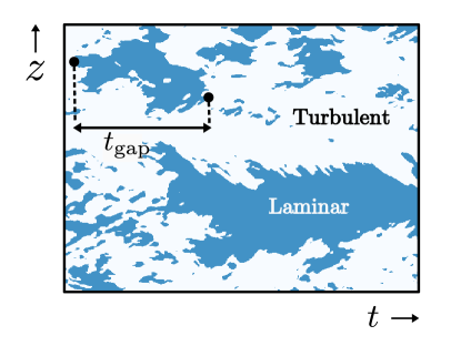
(a)

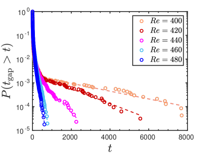
(b)

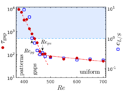
(c)

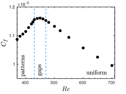
(d)

Figure 4: (a) Same as figure 3b, but illustrating the definition of $t_{\text{gap}}$, the lifetime of a quasi-laminar gap. (b) Survival functions of $t_{\text{gap}}$. After initial steep portions, slopes yield the characteristic times. (c) Evolution with $Re$ of characteristic time $\tau_{\text{gap}}$ and of ratio of large to small scale energy $e_{L/S}$ defined by (7). Both of these quantities present two exponential regimes, with the same slopes and a common crossover at $Re_{\rm gu}$. The horizontal dashed line delimits the region $e_{L/S}>1$, defining $Re_{\rm pg}$ below which regular patterns dominate. We estimate $Re_{\rm pg}\simeq 430$ and $Re_{\rm gu}\simeq 470$ (to two significant figures). (d) Evolution of friction coefficient $C_{f}$ with $Re$, with the three regimes delimited by $Re_{\rm pg}$ and $Re_{\rm gu}$, as defined from (c).

The slope of the exponential tail is extracted at each $Re$ and the resulting characteristic time-scale $\tau_{\text{gap}}$ is shown in figure 4c. The evolution of $\tau_{\rm gap}$ with $Re$ displays two regimes, each with nearly exponential dependence on $Re$, but with very different slopes on the semi-log plot. For $Re\geq 470$, the characteristic lifetimes are $\tau_{\rm gap}=O(10^{2})$ and vary weakly with $Re$. These short timescales correspond to the small white events visible in figure 2a and are associated with low-energy values on the left tails of the PDFs for $e(z,t)$ in figure 3a. Discounting these events, we refer to such states as uniform turbulence. For $Re<470$, $\tau_{\rm gap}$ varies rapidly with $Re$, increasing by two orders of magnitude between $Re=470$ and $Re=380$. The abrupt change in slope seen in figure 4c, which we denote by $Re_{\rm gu}$, marks the transition between gaps and uniform turbulence; we estimate $Re_{\rm gu}=470$ (to two significant figures). We stress that as far as we have been able to determine, there is no critical phenomenon associated with this change of behaviour. That is, the transition is smooth and lacks a true critical point. It is nevertheless evident that the dynamics of quasi-laminar gaps changes significantly in the region of $Re=470$ and therefore it is useful to define a reference Reynolds number marking this change in behaviour.

Note that typical lifetimes of laminar gaps must become infinite by the threshold $Re\simeq 325$ below which turbulence is no longer sustained (Lemoult et al., 2016). (We believe this to be true even for $Re\lesssim 380$ when the permanent banded regime is attained, although this is not shown here.) For this reason, we have restricted our study of gap lifetimes to $Re\gtrsim 380$ and we have limited our maximal simulation time to $\sim 10^{4}$.

To quantify the distinction between localized gaps and patterns, we introduce a variable $e_{L/S}$ as follows. Using the Fourier transform in $z$,

$$\bm{\hat{u}}(x,y,k_{z},t)=\frac{1}{L_{z}}\int_{0}^{L_{z}}\bm{u}(x,y,z,t)e^{-ik_{z}z}\,\text{d}z\>,$$ (5)

we compute the averaged spectral energy

$$\widehat{E}(y,k_{z})\equiv\frac{1}{2}\overline{\bm{\hat{u}}\cdot\bm{\hat{u}}^{\ast}},\qquad\qquad\widehat{E}(k_{z})\equiv\langle\widehat{E}(y,k_{z})\rangle_{y}$$ (6)

where the overbar designates an average in $x$ and $t$. This spectral energy is described in figure 3a of our companion paper Gomé et al. (2023, Part 1). We are interested in the ratio of $\widehat{E}(k_{z})$ at large scales (pattern scale) to small scales (roll-streak scale), as it evolves with $Re$. For this purpose, we define the ratio of large-scale to small-scale maximal energy:

$$e_{L/S}=\frac{\underset{k_{z}<0.5}{\max}\widehat{E}(k_{z})}{\underset{k_{z}\geq 0.5}{\max}\widehat{E}(k_{z})}$$ (7)

The choice of wavenumber $k_{z}=0.5$ to delimit large and small scales comes from the change in sign of non-linear transfers, as established in Gomé et al. (2023, Part 1). This quantity is shown as blue squares in figure 4c and is highly correlated to $\tau_{\rm gap}$. This correlation is in itself a surprising observation for which we have no explanation.

For $Re\gtrsim 430$, we have $e_{L/S}<1$, signaling that the dominant peak in the energy spectrum is at the roll-streak scale, while for $Re\lesssim 430$, the large-scale pattern begins to dominate the streaks and rolls, as indicated by $e_{L/S}>1$ (dashed blue line on figure 4c). Note that $Re=430$ is also the demarcation between unimodal and bimodal PDFs of $e(z,t)$ in figure 3a. The transition from gaps to patterns is smooth. In fact, we do not even observe a qualitative feature sharply distinguishing gaps and patterns. We nevertheless find it useful to define a reference Reynolds number associated to patterns starting to dominate the energy spectrum. This choice has the advantage of yielding a quantitative criterion, which we estimate as $Re_{\rm pg}\simeq 430$ (to two significant figures). We find a similar estimation of the value of $Re$ below which patterns start to dominate via a wavelet-based measurement, see Appendix B.

In addition to the previous quantitative measures, we also extract the friction coefficient. This is defined as the ratio of the mean wall shear stress $\mu U^{\prime}_{\text{wall}}$ to the dynamic pressure $\rho U_{\text{wall}}^{2}/2$, which we write in physical units and then in non-dimensional variables as:

$$C_{f}\equiv\frac{\mu U^{\prime}_{\text{wall}}}{\frac{1}{2}\rho U_{\text{wall}}^{2}}=\frac{2\nu}{hU_{\text{wall}}}\frac{U^{\prime}_{\text{wall}}}{U_{\text{wall}}/h}=\frac{2}{Re}\frac{\partial\left<u_{\text{strm}}\right>_{x,z,t}}{\partial y}\bigg{\rvert}_{\rm wall}$$ (8)

In (8), the dimensional quantities $h$, $\rho$, $\mu$, and $\nu$ are the half-height, the density, and dynamic and kinematic viscosities, and $U_{\rm wall}$ and $U^{\prime}_{\rm wall}$ are the velocity and mean velocity gradient at the wall. We note that the behavior of $C_{f}$ in the transitional region has been investigated in plane channel flow by Shimizu & Manneville (2019) and Kashyap et al. (2020). Our measurements of $C_{f}$ are shown in figure 4d. We distinguish different trends within each of the three regimes defined earlier in figure 4c. In the uniform regime $Re>Re_{\rm gu}=470$, $C_{f}$ increases with decreasing $Re$. In the patterned regime $Re<Re_{\rm pg}=430$, $C_{f}$ decreases with decreasing $Re$. The localised-gap regime $Re_{\rm pg}<Re<Re_{\rm gu}$ connects these two tendencies, with $C_{f}$ reaching a maximum at $Re=450$.

The presence of a region of maximal $C_{f}$ (or equivalently maximal total dissipation) echoes the results on the energy balance presented in Gomé et al. (2023, Part 1): the uniform regime dissipates more energy as $Re$ decreases, up to a point where this is mitigated by the many laminar gaps nucleated. This is presumably due to the mean flow in the turbulent region needing energy influx from gaps to compensate for its increasing dissipation.

3.3 Laminar-turbulent correlation function

The changes in regimes and the distinction between local gaps and patterns can be further studied by measuring the spatial correlation between quasi-laminar regions within the flow. We define

$$\Theta(z,t)=\begin{dcases}1~{}~{}\text{ if }e(z,t)<e_{\rm turb}\text{ (laminar) }\\ 0~{}~{}\text{ otherwise (turbulent) }\end{dcases}$$ (9)

(this is the quantity shown in blue and white in figures 3b and 4a). We then compute its spatial correlation function:

$$C(\delta z)=\frac{\left<{\Theta}(z){\Theta}(z+\delta z)\right>_{z,t}-\left<{\Theta}(z)\right>^{2}_{z,t}}{\left<{\Theta}(z)^{2}\right>_{z,t}-\left<{\Theta}(z)\right>^{2}_{z,t}}.$$ (10)

Along with $(z,t)$ averaging, $C$ is also averaged over multiple realisations of quench experiments. As $\Theta$ is a Heaviside function, $C$ can be understood as the average probability of finding a gap at a distance $\delta z$ from a gap at position $z$. The results are presented in figure 5a. The comparative behaviour of $C$ at near-zero values is enhanced by plotting $\tanh(10~{}C)$ in figure 5b. At long range, $C$ approaches zero with small fluctuations at $Re=480$, a noisy periodicity at $Re=460$, and a nearly periodic behaviour for $Re\leq 420$.

In all cases, $C$ initially decreases from one and reaches a first minimum at $\delta z\simeq 20$, due to the minimal possible size of a turbulent zone that suppresses the creation of neighbouring laminar gaps. $C$ has a prominent local maximum $\delta z_{\rm max}$ right after its initial decrease, at $\delta z_{\rm max}\simeq 32$ at $Re=480$, which increases to $\delta z_{\rm max}\simeq 41$ at $Re=420$. These maxima, shown as coloured circles in figure 5b, indicate that gap nucleation is preferred at distance $\delta z_{\rm max}$ from an existing gap. The increase in $\delta z_{\rm max}$ and in the subsequent extrema as $Re$ is lowered agrees with the trend of increasing wavelength of turbulent bands as $Re$ is decreased in the fully banded regime at lower $Re$ (Prigent et al., 2003; Barkley & Tuckerman, 2005).

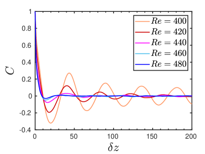
(a)

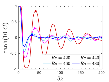
(b)

Figure 5: (a) Gap-to-gap correlation function $C(\delta z)$ defined by (10) for various values of $Re$. (b) For $Re\gtrsim 440$ the weak variation and short-ranged maxima are enhanced by plotting $\tanh(10~{}C(\delta z))$. The dots correspond to the first local maximum, indicating the selection of a finite distance between two local gaps, including at the highest $Re$. Large-scale modulations smoothly leave room to weak short-range interaction as $Re$ increases and the flow visits patterned, local-gap and uniform regimes.

The smooth transition from patterns to uniform flow is confirmed in the behaviour of the correlation function. Large-scale modulations characteristic of the patterned regime gradually disappear with increasing $Re$, as gaps become more and more isolated. Only a weak, finite-length interaction subsists in the local-gap and uniform regimes, and will further disappear with increasing $Re$. This is the selection of this finite gap spacing that we will investigate in §4 and §5.

4 Wavelength selection for turbulent-laminar patterns

In this section, we investigate the existence of a preferred pattern wavelength by using as a control parameter the length $L_{z}$ of the Minimal Band Unit. In a Minimal Band Unit, the system is constrained and the distinction between local gaps and patterns is lost; see section 3 of our companion paper Gomé et al. (2023, Part 1). $L_{z}$ is chosen such as to accommodate at most a single turbulent zone and a single quasi-laminar zone, which due to imposed periodicity, can be viewed as one period of a perfectly periodic pattern. By varying $L_{z}$, we can verify whether a regular pattern of given wavelength $L_{z}$ can emerge from uniform turbulence, disregarding the effect of scales larger than $L_{z}$ or of competition with wavelengths close to $L_{z}$. We refer to these simulations in Minimal Band Units as existence experiments. Indeed, one of the main advantages of the Minimal Band Unit is the ability to create patterns of a given angle and wavelength which may not be stable in a larger domain.

In contrast, in a Long Slender Box, $L_{z}$ is large enough to accommodate multiple bands and possibly even patterns of different wavelengths. An initial condition consisting of a regular pattern of wavelength $\lambda$ can be constructed by concatenating bands produced from a Minimal Band Unit of size $\lambda$. The stability of such a pattern is studied by allowing this initial state to evolve via the non-linear Navier-Stokes equations. Both existence and stability studies can be understood in the framework of the Eckhaus instability (Kramer & Zimmermann, 1985; Ahlers et al., 1986; Tuckerman & Barkley, 1990; Cross & Greenside, 2009).

In previous studies of transitional regimes, Barkley & Tuckerman (2005) studied the evolution of patterns as $L_{z}$ was increased. In Section 4.1, we extend this approach to multiple sizes of the Minimal Band Unit by comparing lifetimes of patterns that naturally arise in this constrained geometry. The stability of regular patterns of various wavelengths will be studied in Long Slender Domains ($L_{z}=400$) in Section 4.2.

4.1 Temporal intermittency of regular patterns in a short-$L_{z}$ box

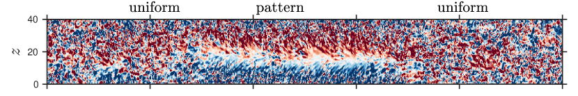
(a)

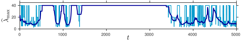
(b)

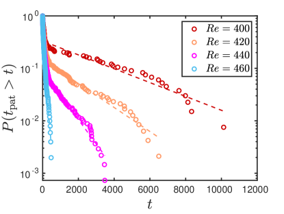
(c)

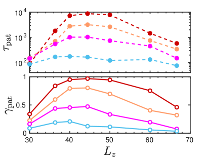
(d)

Figure 6: Pattern lifetimes. (a) Space-time visualization of a metastable pattern in a Minimal Band Unit with $L_{z}=40$ at $Re=440$. Colors show spanwise velocity (blue: $-0.1$, white: 0, red: 0.1). (b) Values of the dominant wavelength $\widehat{\lambda}_{\max}$ (light blue curve) and of its short-time average $\langle\widehat{\lambda}_{\max}\rangle_{t_{a}}$ (dark blue curve) are shown; see (11). A state is defined to be patterned if $\widehat{\lambda}_{\max}=L_{z}$. (c) Survival function of lifetimes of turbulent-laminar patterns in a Minimal Band Unit with $L_{z}=40$ for various $Re$. The pattern lifetimes $t_{\rm pat}$ are the lengths of the time intervals during which $\widehat{\lambda}_{\max}=L_{z}$. (d) Above: characteristic times $\tau_{\rm pat}$ extracted from survival functions as a function of $L_{z}$ and $Re$. Below: intermittency factor for the patterned state $\gamma_{\rm pat}$, which is the fraction of time spent in the patterned state.

Figure 6a shows the formation of a typical pattern in a Minimal Band Unit of size $L_{z}=40$ and at $Re=440$. While the system cannot exhibit the spatial intermittency seen in figure 2c, temporal intermittency is possible and is seen as alternation between uniform turbulence and a pattern. We plot the spanwise velocity at $y=0$ and $x=L_{x}/2$. This is a particularly useful measure of the large-scale flow associated with patterns, seen as red and blue zones surrounding a white quasi-laminar region, i.e. a gap. The patterned state spontaneously emerges from uniform turbulence and remains from $t\simeq 1500$ to $t\simeq 3400$. At $t\simeq 500$, a short-lived gap appears at $z=10$, which can be seen as an attempt to form a pattern.

We characterise the pattern quantitatively as follows. For each time $t$, we compute $|\langle\widehat{\bm{u}}(y=0,k_{z},t)\rangle_{x}|^{2}$, which is the instantaneous energy contained in wavenumber $k_{z}$ at the mid-plane. We then determine the wavenumber that maximises this energy and compute the corresponding wavelength. That is, we define

$$\widehat{\lambda}_{\max}(t)\equiv\frac{2\pi}{\underset{k_{z}>0}{\text{argmax}}\>|{\langle\widehat{\bm{u}}(y=0,k_{z},t)}\rangle_{x}|^{2}}.$$ (11)

The possible values of $\widehat{\lambda}_{\max}$ are integer divisors of $L_{z}$, here 40, 20, 10, etc. Figure 6b presents $\widehat{\lambda}_{\max}$ and its short-time average $\langle\widehat{\lambda}_{\max}\rangle_{t_{a}}$ with $t_{a}=30$ as light and dark blue curves, respectively. When turbulence is uniform, $\widehat{\lambda}_{\max}$ varies rapidly between its discrete allowed values, while $\langle\widehat{\lambda}_{\max}\rangle_{t_{a}}$ fluctuates more gently around 10. The flow state is deemed to be patterned when its dominant mode is $\langle\widehat{\lambda}_{\max}\rangle_{t_{a}}=L_{z}$. The long-lived pattern occurring for $1500\leq t\leq 3400$ in figure 6a is seen as a plateau of $\langle\widehat{\lambda}_{\max}\rangle_{t_{a}}$ in figure 6b. There are other shorter-lived plateaus, notably at for $500\leq t\leq 750$. A similar analysis was carried out by Barkley & Tuckerman (2005); Tuckerman & Barkley (2011) using the Fourier component corresponding to wavelength $L_{z}$ of the spanwise mid-gap velocity.

Figure 6c shows the survival function $t_{\rm pat}$ of the pattern lifetimes obtained from $\langle\widehat{\lambda}_{\max}\rangle_{t_{a}}$ over long simulation times for various $Re$. This measurement differs from figure 4b, which showed lifetimes of gaps in a Long Slender Box and not regular patterns obtained in a Minimal Band Unit. The results are however qualitatively similar, with two characteristic zones in the distribution, as in in figure 4b: at short times, many patterns appear due to fluctuations; while after $t\simeq 200$, the survival functions enter an approximately exponential regime, from which we extract the characteristic times $\tau_{\rm pat}$ by taking the inverse of the slope.

We then vary $L_{z}$, staying within the Minimal Box regime $L_{z}\lesssim 65$ in which only one band can fit. Figure 6d (top) shows that $\tau_{\rm pat}$ presents a broad maximum in $L_{z}$ whose strength and position depend on $Re$: $L_{z}\simeq 42$ at $Re=440$ and $L_{z}\simeq 44$ at $Re=400$. This wavelength corresponds approximately to the natural spacing observed in a Large Slender Box (figure 2). Figure 6d (bottom) presents the fraction of time that is spent in a patterned state, denoted $\gamma_{\rm pat}$, to reflect that this should be thought of as the intermittency factor for the patterned state. The dependence of $\gamma_{\rm pat}$ on $L_{z}$ follows the same trend as $\tau_{\rm pat}$, but less strongly (the scale of the inset is linear, while that for $\tau_{\rm pat}$ is logarithmic).

The results shown in figure 6d complement the Ginzburg-Landau description proposed by Prigent et al. (2003) and Rolland & Manneville (2011). To quantify the bifurcation from featureless to pattern turbulence, these authors defined an order parameter and showed that it has a quadratic maximum at an optimal wavenumber. This is consistent with the approximate quadratic maxima that we observe in $\tau_{\rm pat}$ and in $\gamma_{\rm pat}$ with regard to $L_{z}$. Note that the scale of the pattern can be roughly set from the force balance in the laminar flow regions (Barkley & Tuckerman, 2007), $\lambda\simeq Re\sin\theta/\pi$, which yields a wavelength of 52 at $Re=400$ (close to the value of 44 found in figure 6d).

4.2 Pattern stability in a large domain

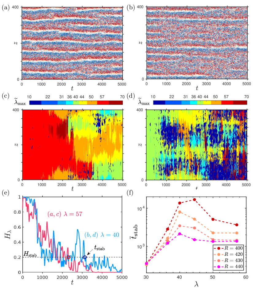
Figure 7: Simulation in a Long Slender Box from a noise-perturbed periodic pattern with (a) initial $\lambda=57$ at $Re=400$ and (b) initial $\lambda=40$ at $Re=430$. Colors show spanwise velocity (red: 0.1, white: 0, blue: $-0.1$). (c) and (d) show the local dominant wavelength $\tilde{\lambda}_{\rm max}(z,t)$ determined by wavelet analysis (see Appendix B) corresponding to the simulations shown in (a) and (b). Color at $t=0$ shows the wavelength $\lambda$ of the initial condition. (e) shows the wavelet-defined $H_{\lambda}(t)$ defined in (12), which quantifies the proportion of the domain that retains initial wavelength $\lambda$ as a function of time for cases (a) and (b). Circles indicate the times for (a) and (b) after which $H_{\lambda}$ is below the threshold value $H_{\rm stab}$ for a sufficiently long time. (f) Ensemble-averaged $\bar{t}_{\text{stab}}$ of the decay time of an imposed pattern of wavelength $\lambda$ for various values of $Re$. The relative stability of a wavelength, whether localised or not, is measured by $\bar{t}_{\text{stab}}$ via the wavelet analysis.

To study the stability of a pattern of wavelength $\lambda$, we prepare an initial condition for a Long Slender Box by concatenating repetitions of a single band produced in a Minimal Band Unit. We add small-amplitude noise to this initial pattern so that the repeated bands do not all evolve identically. Figures 7a and 7b show two examples of such simulations. Depending on the value of $Re$ and of the initial wavelength $\lambda$, the pattern destabilises to either another periodic pattern (figure 7a for $Re=400$) or to localised patterns surrounded by patches of featureless turbulence (figure 7b for $Re=430$).

It can be seen that patterns often occupy only part of the domain. For this reason, we turn to the wavelet decomposition (Meneveau, 1991; Farge, 1992) to quantify patterns locally. In contrast to a Fourier decomposition, the wavelet decomposition quantifies the signal as a function of space and scale. From this, we are able to define a local dominant wavelength, $\widetilde{\lambda}_{\max}(z,t)$, similar in spirit to $\widehat{\lambda}_{\max}(t)$ in (11), but now at each space-time point. (See Appendix B for details.) Figures 7c and 7d show $\widetilde{\lambda}_{\max}(z,t)$ obtained from wavelet analysis of the simulations visualised in figures 7a and 7b.

We now use the local wavelength $\widetilde{\lambda}_{\max}(z,t)$ to quantify the stability of an initial wavelength. We use a domain of length $L_{z}=400$ and we concatenate $n=7$ to 13 repetitions of a single band to produce a pattern with initial wavelength $\lambda(n)\equiv 400/n\simeq 57,50,44\ldots 31$. (We have rounded $\lambda$ to the nearest integer value here and in what follows.) After adding low-amplitude noise, we run a simulation lasting 5000 time units, compute the wavelet transform and calculate from it the local wavelengths $\widetilde{\lambda}_{\max}(z,t)$. We define $\epsilon_{\lambda}\equiv\min((\lambda(n+1)-\lambda(n))/2,(\lambda(n)-\lambda(n-1))/2)$ such that $|\lambda-\widetilde{\lambda}_{\max}(z,t)|<\epsilon_{\lambda}$ if $\widetilde{\lambda}_{\max}$ is closer to $\lambda(n)$ than to its two neighboring values . Finally, in order to measure the proportion of $L_{z}$ in the dominant mode $\widetilde{\lambda}_{\max}$ is $\lambda$, we compute

$$H_{\lambda}(t)=\left\langle\frac{1}{L_{z}}\int_{0}^{L_{z}}\Theta\left(\epsilon_{\lambda}-|\lambda-\widetilde{\lambda}_{\max}(z,t)|\right)~{}\text{d}z\right\rangle_{t_{a}}$$ (12)

where $\Theta$ is the Heaviside function and the short-time average $\left<\cdot\right>_{t_{a}}$ is taken over time $t_{a}=30$ as before. In practice, because patterns in a Long Slender Box still fluctuate in width, a steady pattern may have $H_{\lambda}$ somewhat less than 1. If $H_{\lambda}\ll 1$, a pattern of wavelength $\lambda$ is present in only a very small part of the flow.

Figure 7e shows how wavelet analysis via the Heaviside-like function $H_{\lambda}(t)$ quantifies the relative stability of the pattern in the examples shown in figures 7a and 7b. The flow in figure 7a at $Re=400$ begins with $\lambda=57$, i.e. 7 bands. Figure 7c retains the red color corresponding to $\lambda=57$ over all of the domain for $t\lesssim 1200$ and over most of it until $t\lesssim 2300$. The red curve in figure 7e shows $H_{\lambda}$ decaying quickly and roughly monotonically. One additional gap appears at around $t=2300$ and starting from then, $H_{\lambda}$ remains low. This corresponds to the initial wavelength $\lambda=57$ losing its dominance to $\lambda=40$, 44 and 50 in the visualisation of $\widetilde{\lambda}_{\max}(z,t)$ in figure 7c. By $t=5000$, the flow shows 9 bands with a local wavenumber $\lambda$ between 40 and 50.

The flow in figure 7b at $Re=430$ begins with $\lambda=40$, i.e. 10 bands. Figure 7d shows that the initial light green color corresponding to 40 is retained until $t\lesssim 800$. The blue curve in figure 7e representing $H_{\lambda}$ initially decreases and drops precipitously around $t\simeq 1000$ as several gaps disappear in figure 7b. $H_{\lambda}$ then fluctuates around a finite value, which is correlated to the presence of gaps whose local wavelength is the same as the initial $\lambda$, visible as zones where $\widetilde{\lambda}_{\max}=40$ in figure 7d. The rest of the flow can be mostly seen as locally featureless turbulence, where the dominant wavelength is small ($\widetilde{\lambda}_{\max}\leq 10$). The local patterns fluctuate in width and strength, and $H_{\lambda}$ evolves correspondingly after $t=1000$. The final state reached in figure 7a at $Re=430$ is characterised by the presence of intermittent local gaps.

The lifetime of an initially imposed pattern wavelength $\lambda$ is denoted $t_{\text{stab}}$ and is defined as follows: We first define a threshold $H_{\rm stab}\equiv 0.2$ (marked by a horizontal dashed line on figure 7e). If $H_{\lambda}(t)$ is statistically below $H_{\rm stab}$, the imposed pattern will be considered as unstable. Following this principle, $t_{\text{stab}}$ is defined as the first time $H_{\lambda}$ is below $H_{\rm stab}$, with a further condition to dampen the effect of short-term fluctuations: $t_{\text{stab}}$ must obey $\left<H_{\lambda}(t)\right>_{t\in[t_{\text{stab}},~{}t_{\text{stab}}+2000]}<H_{\rm stab}$, so as to ensure that the final state is on average below $H_{\rm stab}$. The corresponding times in case (a) and (b) are marked respectively by a red and a blue circle in figure 7e.

Repeating this experiment over multiple realisations of the initial pattern (i.e. different noise realisations) yields an ensemble-averaged $\bar{t}_{\text{stab}}$. This procedure estimates the time for an initially regular and dominant wavelength to disappear from the flow domain, regardless of the way in which it does so and of the final state approached. Figure 7f presents the dependence of $\overline{t}_{\text{stab}}$ on $\lambda$ for different values of $Re$. Although our procedure relies on highly fluctuating signals (like those presented on figure 7e) and on a number of arbitrary choices ($H_{\rm stab}$, $\epsilon_{\lambda}$, etc.) that alter the exact values of stability times, we find that the trends visualised in figure 7f are robust. (The sensitivity of $\overline{t}_{\text{stab}}$ with $H_{\rm stab}$ is shown in figure 13b of Appendix B.)

A most-stable wavelength ranging between 40 and 44 dominates the stability times for all the values of $Re$ under study. This is similar to the results from the existence study on figure 6d, which showed a preferred wavelength emerging from the uniform state at around $42$ at $Re=440$. Consistently with what was observed in Minimal Band Units of different sizes, the most stable wavelength grows with decreasing $Re$.

4.3 Discussion

Our study of the existence and stability of large-scale modulations of the turbulent flow is summarised in figure 8. This figure resembles the existence and stability diagrams presented for usual (non-turbulent) hydrodynamic instabilities such as Rayleigh-Bénard convection and Taylor-Couette flow (Busse, 1981; Ahlers et al., 1986; Cross & Greenside, 2009). In classic systems, instabilities appear with increasing control parameter, while here gaps and bands emerge from uniform turbulent flow as $Re$ is lowered. Therefore, we plot the vertical axis in figure 8 with decreasing upwards Reynolds.

We recall that the existence study of $\S$4.1 culminated in the measurement of $\gamma_{\rm pat}(\lambda,Re)$, the fraction of simulation time that is spent in a patterned state, plotted in figure 6d. The parameter values at which $\gamma_{\rm pat}(\lambda,Re)=0.45$ (an arbitrary threshold that covers most of our data range) are shown as black circles in figure 8. The dashed curve is an interpolation of the iso-$\gamma_{\rm pat}$ points and separates two regions, with patterns more likely to exist above the curve than below. The minimum of this curve is estimated to be $\lambda\simeq 42$. This is a preferred wavelength at which patterns first statistically emerge as $Re$ is decreased from large values.

The final result of the stability study in section §4.2, shown in figure 7f, was $\overline{t}_{\text{stab}}(Re,\lambda)$, a typical duration over which a pattern initialised with wavelength $\lambda$ would persist. The colours in figure 8 show $\overline{t}_{\text{stab}}$. The peak in $\overline{t}_{\text{stab}}$ is first discernible at $Re\simeq 440$ and occurs at $\lambda\simeq 40$. The pattern existence and stability zones are similar in shape and in their lack of symmetry with respect to line $\lambda=42$. The transition seen in figures 7a and 7c from $\lambda=57$ to $\lambda=44$ at $Re=400$ corresponds to motion from a light blue to a dark blue area in the top row of figure 8. This change in pattern wavelength resembles the Eckhaus instability which, in classic hydrodynamics, leads to transitions from unstable wavelengths outside a stability band to stable wavelengths inside.

The presence of a most-probable wavelength confirms the initial results of Prigent et al. (2003) and those of Rolland & Manneville (2011). This is also consistent with the instability study of Kashyap et al. (2022) in plane Poiseuille flow. However, contrary to classic pattern-forming instabilities, the turbulent-laminar pattern does not emerge from an exactly uniform state, but instead from a state in which local gaps are intermittent, as established in Section 3. In Section 5, we will emphasise the importance of the mean flow in the wavelength selection that we have described.

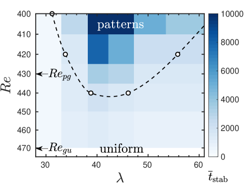
Figure 8: Visualisation of the pattern selection in the phase space $(\lambda,Re)$. Colours show the stability times $\overline{t}_{\text{stab}}$, while open circles are points $\gamma_{\rm pat}(\lambda,Re)=0.45$. The dashed line is an illustrative fit of these points.

5 Optimisation of the large-scale flow

This section is devoted to the dependence of various energetic features of the patterned flow on the domain length $L_{z}$ of a Minimal Band Unit. We fix the Reynolds number at $Re=400$. In the existence study of §4, the wavelength $\lambda\simeq 44$ was found to be selected by patterns. (Recall the uppermost curves corresponding to $Re=400$ in figure 6d.) We will show that this wavelength also extremises quantities in the energy balances of the flow.

5.1 Average energies in the patterned state

We first decompose the flow into a mean and fluctuations, $\bm{u}=\overline{\bm{u}}+\bm{u}^{\prime}$, where the mean (overbar) is taken over the statistically homogeneous directions $x$ and $t$. We compute energies of the total flow $\left<E\right>\equiv\left<\bm{u}\cdot\bm{u}\right>/2$ and of the fluctuations (turbulent kinetic energy) $\left<K\right>\equiv\left<\bm{u}^{\prime}\cdot\bm{u}^{\prime}\right>/2$, where $\left<\cdot\right>$ is the $(x,y,z,t)$ average. Figure 9a shows these quantities as a function of $L_{z}$ for the patterned state at $Re=400$. At $L_{z}=44$, $\left<E\right>$ is maximal and $\left<K\right>$ is minimal. As a consequence, the mean-flow energy $\frac{1}{2}\left<\overline{\bm{u}}\cdot\overline{\bm{u}}\right>=\left<E\right>-\left<K\right>$ is also maximal at $L_{z}=44$. Figure 9a additionally shows average dissipation of the total flow $\left<D\right>\equiv\left<|\nabla\times\bm{u}|^{2}\right>/Re$ and average dissipation of turbulent kinetic energy $\left<\epsilon\right>\equiv\left<|\nabla\times\bm{u}^{\prime}|^{2}\right>/Re$, both of which are minimal at $L_{z}=44$. Note that these total energy and dissipation terms change very weakly with $L_{z}$, with a variation of less than $6\%$.

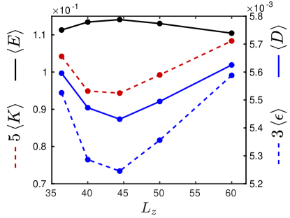
(a)

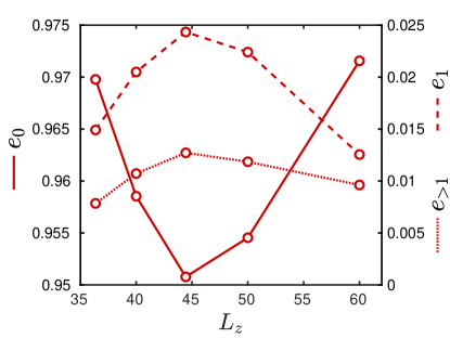
(b)

Figure 9: Energy analysis for the patterned state at $Re=400$ as a function of the size $L_{z}$ of a Minimal Band Unit. (a) Spatially-averaged total energy $\left<E\right>$, mean TKE $\left<K\right>$ ($\times 5$), mean total dissipation $\left<D\right>$, mean turbulent dissipation $\left<\epsilon\right>$ ($\times 3$), for the patterned state at $Re=400$ as a function of $L_{z}$. (b) Energy in each of the $z$-Fourier components of the mean flow (equations (13) and (14)).

The mean flow is further analysed by computing the energy of each spectral component of the mean flow. For this, the $x$, $t$ averaged flow $\overline{\bm{u}}$ is decomposed into Fourier modes in $z$:

$$\overline{\bm{u}}(y,z)=\overline{\bm{u}}_{0}(y)+2\mathcal{R}\left(\overline{\bm{u}}_{1}(y)e^{i2\pi z/L_{z}}\right)+\overline{\bm{u}}_{>1}(y,z)$$ (13)

where $\overline{\bm{u}}_{0}$ is the uniform component of the mean flow, $\overline{\bm{u}}_{1}$ is the trigonometric Fourier coefficient corresponding to $k_{z}=2\pi/L_{z}$ and $\overline{\bm{u}}_{>1}$ is the remainder of the decomposition, for $k_{z}>2\pi/L_{z}$. (We have omitted the hats on the $z$ Fourier components of $\overline{\bm{u}}$.) The energies of the spectral components relative to the total mean energy are

$$e_{0}=\frac{\left<\overline{\bm{u}}_{0}\cdot\overline{\bm{u}}_{0}\right>}{\left<\overline{\bm{u}}\cdot\overline{\bm{u}}\right>},~{}~{}~{}e_{1}=\frac{\left<\overline{\bm{u}}_{1}\cdot\overline{\bm{u}}_{1}\right>}{\left<\overline{\bm{u}}\cdot\overline{\bm{u}}\right>},~{}~{}~{}e_{>1}=\frac{\left<\overline{\bm{u}}_{>1}\cdot\overline{\bm{u}}_{>1}\right>}{\left<\overline{\bm{u}}\cdot\overline{\bm{u}}\right>}$$ (14)

These are presented in figure 9b. It can be seen that $e_{0}\gg e_{1}>e_{>1}$ and also that all have an extremum at $L_{z}=44$. In particular, $L_{z}=44$ minimizes $e_{0}$ ($e_{0}=0.95$) while maximising the trigonometric component ($e_{1}=0.025$) along with the remaining components ($e_{>1}\simeq 0.011$). Note that for a banded state at $Re=350$, $L_{z}=40$, Barkley & Tuckerman (2007) found that $e_{0}\simeq 0.70$, $e_{1}\simeq 0.30$ and $e_{>1}\simeq 0.004$, consistent with a strengthening of the bands as $Re$ is decreased.

5.2 Mean flow spectral balance

We now investigate the spectral contributions to the budget of the mean flow $\overline{\bm{u}}$, dominated by the mean flow’s two main spectral components $\overline{\bm{u}}_{0}$ and $\overline{\bm{u}}_{1}$. The balances can be expressed as in Gomé et al. (2023, Part 1):

$$\widehat{\overline{A}}_{0}-\widehat{\overline{\Pi}}_{0}-\widehat{\overline{D}}_{0}+I=0\text{ for }\overline{\bm{u}}_{0}~{}~{}~{}\text{and}~{}~{}~{}\widehat{\overline{A}}_{1}-\widehat{\overline{\Pi}}_{1}-\widehat{\overline{D}}_{1}=0\text{ for }\overline{\bm{u}}_{1}$$ (15)

where $I$ is the rate of energy injection by the viscous shear, and $\widehat{\overline{\Pi}}_{0}$, $\widehat{\overline{D}}_{0}$ and $\widehat{\overline{A}}_{0}$ stand for, respectively, production, dissipation and advection (i.e. non-linear interaction) contributions to the energy balance of mode $\overline{\bm{u}}_{0}$ and similarly for $\overline{\bm{u}}_{1}$. These are defined by

$$I =\frac{2}{Re}\mathcal{R}\left\{\int_{-1}^{1}\frac{\partial}{\partial y}\left(\widehat{\overline{u}}_{j}^{*}(k_{z}=0)\widehat{\overline{s}}_{yj}(k_{z}=0)\right)\,\text{d}y\right\}=\frac{1}{Re}\left(\frac{\partial\overline{u}_{\text{strm}}}{\partial y}\bigg{\rvert}_{1}+\frac{\partial\overline{u}_{\text{strm}}}{\partial y}\bigg{\rvert}_{-1}\right)$$ (16a)

$$\widehat{\overline{\Pi}}_{0} =\mathcal{R}\left\{\int_{-1}^{1}\frac{\partial\widehat{\overline{u}}_{j}^{*}}{\partial x_{i}}(k_{z}=0)~{}\widehat{\overline{u_{i}^{\prime}u_{j}^{\prime}}}(k_{z}=0)~{}\text{d}y\right\}$$ (16b)

$$\widehat{\overline{D}}_{0} =\frac{2}{Re}\mathcal{R}\left\{\int_{-1}^{1}\widehat{\overline{s}}_{ij}(k_{z}=0)~{}\widehat{\overline{s}}_{ij}^{*}(k_{z}=0)~{}\text{d}y\right\}$$ (16c)

$$\widehat{\overline{A}}_{0} =-\mathcal{R}\left\{\int_{-1}^{1}\widehat{\overline{u}}_{j}^{*}(k_{z}=0)~{}\widehat{\overline{u}_{i}\frac{\partial\overline{u}_{j}}{\partial x_{i}}}(k_{z}=0)~{}\text{d}y\right\}$$ (16d)

where $\mathcal{R}$ denotes the real part. We define $\widehat{\overline{\Pi}}_{1}$, $\widehat{\overline{D}}_{1}$ and $\widehat{\overline{A}}_{1}$ similarly by replacing $k_{z}=0$ by $k_{z}=2\pi/L_{z}$ in (16a)-(16d).

We recall two main results from Gomé et al. (2023, Part 1): first, $\widehat{\overline{A}}_{1}\simeq-\widehat{\overline{A}}_{0}$. This term represents the energetic transfer between modes $\overline{\bm{u}}_{0}$ and $\overline{\bm{u}}_{1}$ via the self-advection of the mean flow (the energetic spectral influx from $(\overline{\bm{u}}\cdot\nabla)\overline{\bm{u}}$). Second, $\widehat{\overline{\Pi}}_{1}<0$, and this term approximately balances the negative part of TKE production. This is an energy transfer from turbulent fluctuations to the component $\overline{\bm{u}}_{1}$ of the mean flow.

Each term contributing to the balance of $\overline{\bm{u}}_{0}$ and $\overline{\bm{u}}_{1}$ is shown as a function of $L_{z}$ in figures 10a and 10b. We do not show $\widehat{\overline{A}}_{0}$ because $\widehat{\overline{A}}_{0}\simeq-\widehat{\overline{A}}_{1}$.

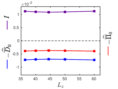
(a)

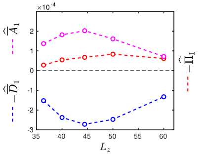
(b)

Figure 10: Spectral energy balance of the mean flow components (a) $\overline{\bm{u}}_{0}$ (uniform component) and (b) $\overline{\bm{u}}_{1}$ (large-scale flow along the laminar-turbulent interface). See equation (15). Advection and dissipation of the large-scale flow, $\widehat{\overline{A}}_{1}$ and $\widehat{\overline{D}}_{1}$, show the strongest variations with $L_{z}$ and are optimal at the preferred wavelength $L_{z}\simeq 44$.

We obtain the following results:

1. Production $\widehat{\overline{\Pi}}_{0}$, dissipation $\widehat{\overline{D}}_{0}$ and energy injection $I$ are nearly independent of $L_{z}$, varing by no more than 6% over the range shown. These $k_{z}=0$ quantities correspond to uniform fields in $z$ and hence it is unsurprising that they depend very little on $L_{z}$.

2. The non-linear term $\widehat{\overline{A}}_{1}\simeq-\widehat{\overline{A}}_{0}$, i.e. the transfer from $\overline{\bm{u}}_{0}$ to $\overline{\bm{u}}_{1}$ which is the principal source of energy of $\overline{\bm{u}}_{1}$, varies strongly with $L_{z}$ and has a maximum at $L_{z}\simeq 44$. This is the reason for which $\overline{\bm{u}}_{0}$ is minimised by $L_{z}\simeq 44$ (see figure 9b): more energy is transferred from $\overline{\bm{u}}_{0}$ to $\overline{\bm{u}}_{1}$.

3. Production $\widehat{\overline{\Pi}}_{1}$ increases with $L_{z}$ and does not show an extremum at $L_{z}\simeq 44$ (it instead has a weak maximum at $L_{z}\simeq 50$). In all cases, $\widehat{\overline{\Pi}}_{1}<\widehat{\overline{A}}_{1}$: the TKE feedback on the mean flow, although present, is not dominant and not selective.

4. Dissipation $\widehat{\overline{D}}_{1}$ accounts for the remaining budget and its extremum at $L_{z}\simeq 44$ corresponds to maximal dissipation.

The turbulent kinetic energy balance is also modified with changing $L_{z}$. This is presented in Appendix C. The impact of TKE is however secondary, because of the results established in item (3).

6 Conclusion and discussion

We have explored the appearance of patterns from uniform turbulence in plane Couette flow at $Re\leq 500$. We used numerical domains of different sizes to quantify the competition between featureless (or uniform) turbulence and (quasi-) laminar gaps. In Minimal Band Units, intermittency reduces to a random alternation between two states: uniform or patterned. In large slender domains, however, gaps nucleate randomly and locally in space, and the transition to patterns takes place continuously via the regimes presented in Section 3: the uniform regime in which gaps are rare and short-lived (above $Re\simeq 470$), and another regime ($Re<470$) in which gaps are more numerous and long-lived. Below $Re\simeq 430$, the large-scale spacing of these gaps starts to dominate the energy spectrum, which is a possible demarcation of the patterned regime. With further decrease in $Re$, gaps eventually fill the entire flow domain, forming regular patterns. The distinction between these regimes is observed in both gap lifetime and friction factor.

Spatially isolated gaps were already observed by Prigent et al. (2003), Barkley & Tuckerman (2005) and Rolland & Manneville (2011). (See also Manneville (2015, 2017) and references therein.) Our results confirm that pattern emergence, mediated by randomly-nucleated gaps, is necessarily more complex than the supercritical Ginzburg-Landau framework initially proposed by Prigent et al. (2003) and later developed by Rolland & Manneville (2011). However, this does not preclude linear processes in the appearance of patterns, such as those reported by Kashyap et al. (2022) from an ensemble-averaged linear response analysis.

The intermittency between uniform turbulence and gaps that we quantify here in the range $380\lesssim Re\lesssim 500$ is not comparable to that between laminar flow and bands present for $325\lesssim Re\lesssim 340$. The latter is a continuous phase transition in which the laminar flow is absorbing: laminar regions cannot spontaneously develop into turbulence and can only become turbulent by contamination from neighbouring turbulent flow. This is connected to the existence of a critical point at which the correlation length diverges with a power-law scaling with $Re$, as characterised by important past studies (Shi et al., 2013; Chantry et al., 2017; Lemoult et al., 2016) which demonstrated a connection to directed percolation. The emergence of gaps from uniform turbulence is of a different nature. Neither uniform turbulence nor gaps are absorbing states, since gaps can always appear spontaneously and can also disappear, returning the flow locally to a turbulent state. While the lifetimes of quasi-laminar gaps do exhibit an abrupt change in behaviour at $Re=470$ (figure 4c), we observe no evidence of critical phenomena associated with the emergence of gaps from uniform turbulence. Hence, the change in behaviour appears to be in fact smooth. This is also true in pipe flow where quasi-laminar gaps form, but not patterns (Avila & Hof, 2013; Frishman & Grafke, 2022).

We used the pattern wavelength as a control parameter, via either the domain size or the initial condition, to investigate the existence of a preferred pattern wavelength. We propose that the finite spacing between gaps, visible in both local gaps and patterned regimes, is selected by the preferred size of their associated large-scale flow. Once gaps are sufficiently numerous and patterns are established, their average wavelength increases with decreasing $Re$, with changes in wavelength in a similar vein to the Eckhaus picture.

The influence of the large-scale flow in wavelength selection is analysed in Section 5, where we carried out a spectral analysis like that in Gomé et al. (2023, Part 1) for various sizes of the Minimal Band Unit. In particular, we investigated the roles of the turbulent fluctuations and of the mean flow, which is in turn decomposed into its uniform component $\overline{\bm{u}}_{0}$ and its trigonometric component $\overline{\bm{u}}_{1}$, associated to the large-scale flow along the laminar-turbulent interface. Our results demonstrate a maximisation of the energy and dissipation of $\overline{\bm{u}}_{1}$ by the wavelength naturally preferred by the flow, and this is primarily associated to an optimisation of the advective term $(\overline{\bm{u}}\cdot\nabla)\overline{\bm{u}}$ in the mean flow equation. This term redistributes energy between modes $\overline{\bm{u}}_{0}$ and $\overline{\bm{u}}_{1}$ and is mostly responsible for energising the large-scale along-band flow. Turbulent fluctuations are of secondary importance in driving the large-scale flow and do not play a significant role in the wavelength selection. Our results of maximal transport of momentum and dissipation of the large-scale flow are therefore analogous to the principles mentioned by Malkus (1956) and Busse (1981). Explaining this observation from first principles remains a prodigious task.

It is essential to understand the creation of the large-scale flow around a randomly emerging laminar hole. The statistics obtained in our tilted configuration should be extended to large streamwise-spanwise domains, where short-lived and randomly-nucleated holes might align in the streamwise direction (Manneville, 2017, Fig. 5). This presumably occurs at $Re$ above the long-lived-gap regime, in which the two gap orientations $\pm\theta$ compete. The selected pattern angle might also maximise the dissipation of the large-scale flow, similarly to what we found for the preferred wavelength. Furthermore, a more complete dynamical picture of gap creation is needed. The excitable model of Barkley (2011a) might provide a proper framework, as it accounts for both the emergence of anti-puffs (Frishman & Grafke, 2022) and of periodic solutions (Barkley, 2011b). Connecting this model to the Navier-Stokes equations is, however, a formidable challenge. Our work emphasises the necessity of including the effects of the advective large-scale flow (Barkley & Tuckerman, 2007; Duguet & Schlatter, 2013; Klotz et al., 2021; Marensi et al., 2022) to adapt this model to the establishment of the turbulent-laminar patterns of both preferred wavelength and angle observed in planar shear flows.

Declaration of Interests

The authors report no conflict of interest.

Appendix A Laminar and turbulent distributions in pipe vs Couette flows.

From figures 3c and 3d of the main text, both distributions of laminar or turbulent lengths, $L_{\rm lam}$ and $L_{\rm turb}$, are exponential for large enough lengths, similarly to pipe (Avila & Hof, 2013). It is however striking that the distributions of $L_{\rm lam}$ and $L_{\rm turb}$ have different shapes for $L_{\rm lam}$ or $L_{\rm turb}>10$ in plane Couette flow: $L_{\rm lam}$ shows a sharper distribution, whereas $L_{\rm turb}$ is more broadly distributed. We present on figures 11a and 11b the cumulative distributions of $L_{\rm lam}$ and $L_{\rm turb}$ for a complementary analysis.

We focus on the characteristic length $l_{\rm turb}^{*}$ or $l_{\rm lam}^{*}$ for which $P(L_{\rm lam}>l_{\rm lam}^{*})=P(L_{\rm turb}>l_{\rm turb}^{*})=10^{-2}$: for example, $l_{\rm lam}^{*}=15.5$ and $l_{\rm turb}^{*}=26.5$ at $Re=440$; $l_{\rm lam}^{*}=23.4$ and $l_{\rm turb}^{*}=30.3$ at $Re=400$. We see that $l_{\rm turb}^{*}$ and $l_{\rm lam}^{*}$ are of the same order of magnitude. This differs from the same measurement in pipe flow, carried out by Avila & Hof (2013, Fig. 2): $l_{\rm lam}^{*}=6$ and $l_{\rm turb}^{*}\simeq 50$ at $Re=2800$; $l_{\rm lam}^{*}\simeq 17$ and $l_{\rm turb}^{*}\simeq 160$ at $Re=2500$ (as extracted from their figure 2.). This confirms that turbulent and laminar spacings are of the same order of magnitude in plane Couette flow, contrary to pipe flow.

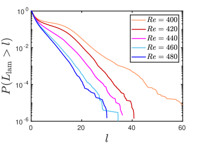
(a)

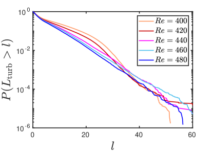
(b)

Figure 11: Cumulative distribution of (a) laminar gaps and (b) turbulent zones, for various $Re$.

Appendix B Wavelet transform

We introduce the one-dimensional continuous wavelet transform of the velocity $\bm{u}(z,t)$ taken along the line $(x,y)=(L_{x}/2,0)$:

$$\tilde{\bm{u}}(z,r,t)=C_{\psi}^{-1/2}r^{-1/2}\int_{0}^{L_{z}}\psi^{*}\left(\frac{z^{\prime}-z}{r}\right)\bm{u}(z^{\prime},t)dz^{\prime}$$ (17)

Here $\psi$ is the Morlet basis function, defined in Fourier space as $\hat{\psi}(k)=\pi^{-1/4}e^{-(k-k_{\psi})^{2}/2}$ for $k>0$. Its central wavenumber is $k_{\psi}=6/\Delta z$, where $\Delta z$ is the grid spacing. The scale factor $r$ is related to wavelength via $\lambda\simeq 2\pi r/k_{\psi}$. $C_{\psi}\equiv\int|k|^{-1}|\hat{\psi}(k)|^{2}\text{d}k$ is a normalization constant. Tildes are used to designate wavelet transformed quantities. The inverse transform is:

$$\bm{u}(z,t)=C_{\psi}^{-1/2}\int_{0}^{\infty}\int_{-\infty}^{\infty}\>r^{-1/2}\psi\left(\frac{z-z^{\prime}}{r}\right)\tilde{\bm{u}}(z^{\prime},r,t)\>\frac{dz^{\prime}~{}dr}{r^{2}}$$ (18)

The wavelet transform is related to the Fourier transform in $z$ by:

$$\tilde{\bm{u}}(z,r,t)=\frac{1}{2\pi}C_{\psi}^{-1/2}r^{1/2}\int_{-\infty}^{\infty}\widehat{\psi}(r\,k_{z})\widehat{\bm{u}}(k_{z},t)e^{ik_{z}z}\text{d}k_{z}$$ (19)

We then define the most energetic instantaneous wavelength as:

$$\widetilde{\lambda}_{\max}(z,t)=\frac{2\pi}{k_{\psi}}~{}\underset{r}{\text{argmax}}~{}|\tilde{\bm{u}}(z,r,t)|^{2}$$ (20)

The characteristic evolution of $\widetilde{\lambda}_{\max}(z,t)$ is illustrated in figure 12b for the flow case corresponding to figure 12a. Regions in which $\widetilde{\lambda}_{\max}$ is large $(>10)$ and dominated by a single value correspond to the local patterns observed in figure 12a. In contrast, in regions where $\widetilde{\lambda}_{\max}$ is small $(<10)$ and fluctuating, the turbulence is locally uniform.

This space-time intermittency of the patterns is quantified by measuring

$$f_{L/S}=\left<\Theta(\widetilde{\lambda}_{\max}(z,t)-10)\right>_{z,t}$$ (21)

and is shown in figure 13a as a function of $Re$.

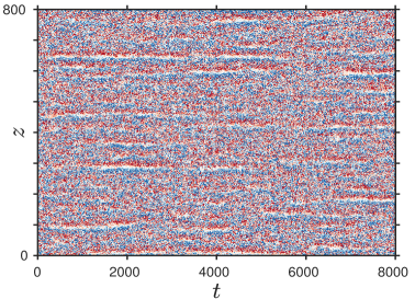
(a)

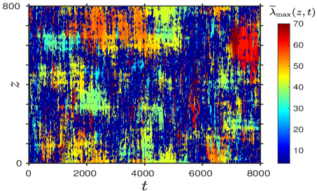
(b)

Figure 12: Space-time visualisation of a quench experiment at $Re=430$: (a) spanwise velocity (blue: $-0.2$, white: 0, red: 0.2), (b) $\widetilde{\lambda}_{\max}(z,t)$ defined by (20). $\widetilde{\lambda}_{\max}(z,t)$ (b) quantifies the presence of local large-scale modulations within the flow. Dark blue zones where $\widetilde{\lambda}_{\max}(z,t)<10$ correspond to locally featureless turbulence in (a). Large-scale modulation of gaps at different wavelengths are visible as the green-to-red spots in (b).

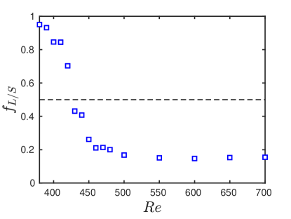
(a)

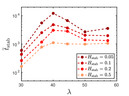
(b)

Figure 13: (a) Space-time fraction of large to small wavelengths obtained by wavelet transform. $f_{L/S}$ crosses 0.5 at $Re\simeq 427\simeq Re_{\rm pg}$. (b) Sensitivity of the stability analysis in 4.2 with regard to threshold $H_{\rm stab}$, at $Re=430$.

Appendix C Turbulent kinetic energy balance for various $L_{z}$

In this appendix, we address the balance of turbulent kinetic energy $\widehat{K}(k_{z})$, written here in $y$-integrated form at a specific mode $k_{z}$ (see equation (5.3) of Gomé et al. (2023, Part 1) and the methodology in, e.g., Bolotnov et al. (2010); Lee & Moser (2015); Mizuno (2016); Cho et al. (2018)):

$$0=\widehat{\Pi}-\widehat{D}+\widehat{A}+\widehat{T}_{nl}$$ (22)

where the variables in (22) indicate $y$-integrated quantities:

$$\widehat{\Pi}(k_{z})\equiv-\mathcal{R}\left\{\int_{-1}^{1}\overline{\widehat{u_{j}^{\prime}}^{*}\widehat{\overline{u}_{i}\frac{\partial u_{j}^{\prime}}{\partial x_{i}}}}~{}\text{d}y\right\},~{}~{}~{}~{}\widehat{D}(k_{z})\equiv\frac{2}{Re}\int_{-1}^{1}\overline{\widehat{s_{ij}^{\prime}}\widehat{s_{ij}^{\prime}}^{*}}~{}\text{d}y,$$

$$\widehat{T}_{nl}(k_{z})\equiv-\mathcal{R}\left\{\int_{-1}^{1}\overline{\widehat{u_{j}^{\prime}}^{*}\widehat{u_{i}^{\prime}\frac{\partial u_{j}^{\prime}}{\partial x_{i}}}}~{}\text{d}y\right\},~{}~{}~{}~{}\widehat{A}(k_{z})\equiv-\mathcal{R}\left\{\int_{-1}^{1}\overline{\widehat{u_{j}^{\prime}}^{*}\widehat{\overline{u}_{i}\frac{\partial u_{j}^{\prime}}{\partial x_{i}}}}~{}\text{d}y\right\}$$ (23)

respectively standing for production, dissipation, triadic interaction and advection terms. We recall that $\overline{(\cdot)}$ is an average in $(x,t)$. The $y$ evolution of the energy balance was analysed in Gomé et al. (2023, Part 1).

Gomé et al. (2023, Part 1) reported robust negative production at large scales, along with inverse non-linear transfers to large scales. If $k_{\text{rolls}}=1.41$ denotes the scale of rolls and streaks, this inverse transfer occurs for $k_{z}<k_{\text{LS}}=0.94$, while a downward transfer occurs for $k_{z}>k_{\text{SS}}=3.6$ (We refer the reader to figure 5 of Gomé et al. (2023, Part 1)). This spectral organization of the energy balance will be quantified by the following transfer terms arising from (23):

$$\widehat{T}_{LS}\equiv\sum_{k_{z}=0}^{k_{\text{LS}}}\widehat{T}_{nl}(k_{z}),~{}~{}~{}\widehat{T}_{SS}\equiv\sum_{k_{z}=k_{\text{SS}}}^{\infty}\widehat{T}_{nl}(k_{z}),~{}~{}~{}\widehat{D}_{LS}\equiv\sum_{k_{z}=0}^{k_{\text{LS}}}\widehat{D}(k_{z}),~{}~{}~{}\widehat{A}_{LS}\equiv\sum_{k_{z}=0}^{k_{\text{LS}}}\widehat{A}(k_{z})$$ (24)

$\widehat{T}_{LS}$ quantifies transfer to large scales, $\widehat{T}_{SS}$ the transfer to small scales, $\widehat{D}_{LS}$ the dissipation at large scales, and $\widehat{A}_{LS}$ is a transfer of energy from the mean flow to the large fluctuating scales. Large-scale production is not shown here, as we presented in figure 10b a similar measurement of large-scale turbulent transfer to the mean flow, via $\widehat{\overline{\Pi}}_{1}$.

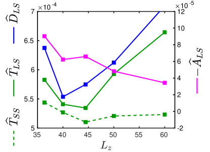
Figure 14: Evolution of the large-scale TKE balance with $L_{z}$ (24).

The variables defined in (24) are displayed in figure 14 as a function of $L_{z}$. $\widehat{T}_{LS}$ is minimal at $L_{z}\simeq 44$. $\widehat{D}_{LS}$ is minimal at $L_{z}\simeq 40$. Contrary to $\widehat{T}_{LS}$, $\widehat{T}_{SS}$ is relatively constant with $L_{z}$ (green dashed line in figure 14), with a variation of around $6\%$. This demonstrates that transfers to small scales are unchanged with $L_{z}$. Large-scale TKE advection decays with increasing $L_{z}$ hence it does not play a role in the preference of a wavelength. Our results show that the balance at large-scale is minimised around $L_{z}\simeq 44$, confirming the less important role played by turbulent fluctuations in the wavelength selection, compared to that of the mean-flow advection reported in the main text.

References

- Ahlers et al. (1986) Ahlers, Guenter, Cannell, David S, Dominguez-Lerma, Marco A & Heinrichs, Richard 1986 Wavenumber selection and Eckhaus instability in Couette-Taylor flow. Physica D 23 (1-3), 202–219.
- Andereck et al. (1986) Andereck, C David, Liu, SS & Swinney, Harry L 1986 Flow regimes in a circular Couette system with independently rotating cylinders. J. Fluid Mech. 164, 155–183.
- Avila & Hof (2013) Avila, Marc & Hof, Björn 2013 Nature of laminar-turbulence intermittency in shear flows. Phys. Rev. E 87 (6), 063012.
- Barkley (2006) Barkley, Dwight 2006 Linear analysis of the cylinder wake mean flow. Europhys. Lett. 75 (5), 750.
- Barkley (2011a) Barkley, Dwight 2011a Simplifying the complexity of pipe flow. Phys. Rev. E 84 (1), 016309.
- Barkley (2011b) Barkley, Dwight 2011b Modeling the transition to turbulence in shear flows. J. Phys. Conf. Ser. 318 (3), 032001.
- Barkley (2016) Barkley, Dwight 2016 Theoretical perspective on the route to turbulence in a pipe. J. Fluid Mech. 803, P1.
- Barkley & Tuckerman (2005) Barkley, Dwight & Tuckerman, Laurette S 2005 Computational study of turbulent-laminar patterns in Couette flow. Phys. Rev. Lett. 94 (1), 014502.
- Barkley & Tuckerman (2007) Barkley, Dwight & Tuckerman, Laurette S 2007 Mean flow of turbulent–laminar patterns in plane Couette flow. J. Fluid Mech. 576, 109–137.
- Bengana & Tuckerman (2021) Bengana, Yacine & Tuckerman, Laurette S 2021 Frequency prediction from exact or self-consistent mean flows. Physical Review Fluids 6 (6), 063901.
- Bolotnov et al. (2010) Bolotnov, Igor A, Lahey Jr, Richard T, Drew, Donald A, Jansen, Kenneth E & Oberai, Assad A 2010 Spectral analysis of turbulence based on the DNS of a channel flow. Computers & Fluids 39 (4), 640–655.
- Busse (1981) Busse, Friedrich H 1981 Transition to turbulence in Rayleigh-Bénard convection. In Hydrodynamic instabilities and the transition to turbulence, pp. 97–137. Springer.
- Chantry et al. (2017) Chantry, Matthew, Tuckerman, Laurette S & Barkley, Dwight 2017 Universal continuous transition to turbulence in a planar shear flow. J. Fluid Mech. 824, R1.
- Cho et al. (2018) Cho, Minjeong, Hwang, Yongyun & Choi, Haecheon 2018 Scale interactions and spectral energy transfer in turbulent channel flow. J. Fluid Mech. 854, 474–504.
- Coles & van Atta (1966) Coles, Donald & van Atta, Charles 1966 Progress report on a digital experiment in spiral turbulence. AIAA Journal 4 (11), 1969–1971.
- Cross & Greenside (2009) Cross, Michael & Greenside, Henry 2009 Pattern Formation and Dynamics in Nonequilibrium Systems. Cambridge University Press.
- Dong (2009) Dong, S 2009 Evidence for internal structures of spiral turbulence. Phys. Rev. E 80 (6), 067301.
- Duguet & Schlatter (2013) Duguet, Yohann & Schlatter, Philipp 2013 Oblique laminar-turbulent interfaces in plane shear flows. Phys. Rev Lett. 110 (3), 034502.
- Duguet et al. (2010) Duguet, Yohann, Schlatter, Philipp & Henningson, Dan S 2010 Formation of turbulent patterns near the onset of transition in plane Couette flow. J. Fluid Mech. 650, 119–129.
- Farge (1992) Farge, Marie 1992 Wavelet transforms and their applications to turbulence. Annu. Rev. Fluid Mech. 24 (1), 395–458.
- Frishman & Grafke (2022) Frishman, Anna & Grafke, Tobias 2022 Dynamical landscape of transitional pipe flow. Phys. Rev. E 105, 045108.
- Gibson et al. (2019) Gibson, J.F., Reetz, F., Azimi, S., Ferraro, A., Kreilos, T., Schrobsdorff, H., Farano, M., A.F. Yesil, S. S. Schütz, Culpo, M. & Schneider, T.M. 2019 Channelflow 2.0. Manuscript in preparation, see channelflow.ch.
- Gomé et al. (2023) Gomé, Sébastien, Tuckerman, Laurette S & Barkley, Dwight 2023 Patterns in transitional turbulence. Part 1. Energy transfer and mean-flow interaction. J. Fluid Mech. 964, A16.
- Hof et al. (2010) Hof, Björn, De Lozar, Alberto, Avila, Marc, Tu, Xiaoyun & Schneider, Tobias M 2010 Eliminating turbulence in spatially intermittent flows. Science 327 (5972), 1491–1494.
- Kashyap (2021) Kashyap, Pavan 2021 Subcritical transition to turbulence in wall-bounded shear flows: spots, pattern formation and low-order modelling. PhD thesis, Université Paris-Saclay.
- Kashyap et al. (2020) Kashyap, Pavan V, Duguet, Yohann & Dauchot, Olivier 2020 Flow statistics in the transitional regime of plane channel flow. Entropy 22 (9), 1001.
- Kashyap et al. (2022) Kashyap, Pavan V, Duguet, Yohann & Dauchot, Olivier 2022 Linear instability of turbulent channel flow. arXiv:2205.05652 .
- Klotz et al. (2022) Klotz, Lukasz, Lemoult, Grégoire, Avila, Kerstin & Hof, Björn 2022 Phase transition to turbulence in spatially extended shear flows. Phys. Rev. Lett. 128 (1), 014502.
- Klotz et al. (2021) Klotz, Lukasz, Pavlenko, AM & Wesfreid, JE 2021 Experimental measurements in plane Couette–Poiseuille flow: dynamics of the large-and small-scale flow. J. Fluid Mech. 912.
- Kramer & Zimmermann (1985) Kramer, Lorenz & Zimmermann, Walter 1985 On the Eckhaus instability for spatially periodic patterns. Physica D 16 (2), 221–232.
- Lee & Moser (2015) Lee, Myoungkyu & Moser, Robert D 2015 Direct numerical simulation of turbulent channel flow up to . J. Fluid Mech. 774, 395–415.
- Lemoult et al. (2016) Lemoult, Grégoire, Shi, Liang, Avila, Kerstin, Jalikop, Shreyas V, Avila, Marc & Hof, Björn 2016 Directed percolation phase transition to sustained turbulence in Couette flow. Nature Physics 12 (3), 254.
- Malkus (1956) Malkus, WVR 1956 Outline of a theory of turbulent shear flow. J. Fluid Mech. 1 (5), 521–539.
- Malkus (1954) Malkus, Willem VR 1954 The heat transport and spectrum of thermal turbulence. Proc. Roy. Soc. A 225 (1161), 196–212.
- Manneville (2012) Manneville, Paul 2012 Turbulent patterns in wall-bounded flows: A Turing instability? Europhys. Lett. 98 (6), 64001.
- Manneville (2015) Manneville, Paul 2015 On the transition to turbulence of wall-bounded flows in general, and plane Couette flow in particular. Eur. J Mech. B Fluids 49, 345–362.
- Manneville (2017) Manneville, Paul 2017 Laminar-turbulent patterning in transitional flows. Entropy 19 (7), 316.
- Marensi et al. (2022) Marensi, Elena, Yalnız, Gökhan & Hof, Björn 2022 Dynamics and proliferation of turbulent stripes in channel and couette flow. arXiv preprint arXiv:2212.12406 .
- Markeviciute & Kerswell (2022) Markeviciute, Vilda K & Kerswell, Rich R 2022 Improved assessment of the statistical stability of turbulent flows using extended Orr-Sommerfeld stability analysis. arXiv:2201.01540 .
- Meneveau (1991) Meneveau, Charles 1991 Analysis of turbulence in the orthonormal wavelet representation. J. Fluid Mech. 232, 469–520.
- Meseguer et al. (2009) Meseguer, Alvaro, Mellibovsky, Fernando, Avila, Marc & Marques, Francisco 2009 Instability mechanisms and transition scenarios of spiral turbulence in Taylor-Couette flow. Phys. Rev. E 80 (4), 046315.
- Mihelich et al. (2017) Mihelich, Martin, Faranda, Davide, Paillard, Didier & Dubrulle, Bérengère 2017 Is turbulence a state of maximum energy dissipation? Entropy 19 (4), 154.
- Mizuno (2016) Mizuno, Yoshinori 2016 Spectra of energy transport in turbulent channel flows for moderate Reynolds numbers. J. Fluid Mech. 805, 171–187.
- Moxey & Barkley (2010) Moxey, David & Barkley, Dwight 2010 Distinct large-scale turbulent-laminar states in transitional pipe flow. Proc. Nat. Acad. Sci. 107 (18), 8091–8096.
- Nagata (1990) Nagata, Masato 1990 Three-dimensional finite-amplitude solutions in plane Couette flow: bifurcation from infinity. J. Fluid Mech. 217, 519–527.
- Ozawa et al. (2001) Ozawa, Hisashi, Shimokawa, Shinya & Sakuma, Hirofumi 2001 Thermodynamics of fluid turbulence: A unified approach to the maximum transport properties. Phys. Rev. E 64 (2), 026303.
- Paranjape et al. (2020) Paranjape, Chaitanya S, Duguet, Yohann & Hof, Björn 2020 Oblique stripe solutions of channel flow. J. Fluid Mech. 897, A7.
- Parker & Krommes (2013) Parker, Jeffrey B & Krommes, John A 2013 Zonal flow as pattern formation. Phys. Plasmas 20 (10), 100703.
- Prigent et al. (2003) Prigent, Arnaud, Grégoire, Guillaume, Chaté, Hugues & Dauchot, Olivier 2003 Long-wavelength modulation of turbulent shear flows. Physica D 174 (1-4), 100–113.
- Prigent et al. (2002) Prigent, Arnaud, Grégoire, Guillaume, Chaté, Hugues, Dauchot, Olivier & van Saarloos, Wim 2002 Large-scale finite-wavelength modulation within turbulent shear flows. Phys. Rev. Lett. 89 (1), 014501.
- Reetz et al. (2019) Reetz, Florian, Kreilos, Tobias & Schneider, Tobias M 2019 Exact invariant solution reveals the origin of self-organized oblique turbulent-laminar stripes. Nature communications 10 (1), 2277.
- Reynolds (1883) Reynolds, Osborne 1883 An experimental investigation of the circumstances which determine whether the motion of water shall be direct or sinuous, and of the law of resistance in parallel channels. Phil. Trans. R. Soc. Lond. 174, 935—982.
- Reynolds & Tiederman (1967) Reynolds, WC & Tiederman, WG 1967 Stability of turbulent channel flow, with application to malkus’s theory. J. Fluid Mech. 27 (2), 253–272.
- Riecke & Paap (1986) Riecke, Hermann & Paap, Hans-Georg 1986 Stability and wave-vector restriction of axisymmetric Taylor vortex flow. Phys. Rev. A 33 (1), 547.
- Rolland & Manneville (2011) Rolland, Joran & Manneville, Paul 2011 Ginzburg–Landau description of laminar-turbulent oblique band formation in transitional plane Couette flow. Eur. Phys. J. B 80 (4), 529–544.
- Samanta et al. (2011) Samanta, Devranjan, De Lozar, Alberto & Hof, Björn 2011 Experimental investigation of laminar turbulent intermittency in pipe flow. J. Fluid Mech. 681, 193–204.
- Shi et al. (2013) Shi, Liang, Avila, Marc & Hof, Björn 2013 Scale invariance at the onset of turbulence in Couette flow. Phys. Rev. Lett. 110 (20), 204502.
- Shimizu & Manneville (2019) Shimizu, Masaki & Manneville, Paul 2019 Bifurcations to turbulence in transitional channel flow. Phys. Rev. Fluids 4, 113903.
- Srinivasan & Young (2012) Srinivasan, Kaushik & Young, W.R. 2012 Zonostrophic instability. J. Atmos. Sci. 69 (5), 1633–1656.
- Tobias & Marston (2013) Tobias, SM & Marston, JB 2013 Direct statistical simulation of out-of-equilibrium jets. Phys. Rev. Lett. 110 (10), 104502.
- Tsukahara et al. (2005) Tsukahara, Takahiro, Seki, Yohji, Kawamura, Hiroshi & Tochio, Daisuke 2005 DNS of turbulent channel flow at very low Reynolds numbers. In Fourth International Symposium on Turbulence and Shear Flow Phenomena. Begel House Inc. arXiv:1406.0248.
- Tuckerman & Barkley (1990) Tuckerman, Laurette S & Barkley, Dwight 1990 Bifurcation analysis of the Eckhaus instability. Physica D 46 (1), 57–86.
- Tuckerman & Barkley (2011) Tuckerman, Laurette S & Barkley, Dwight 2011 Patterns and dynamics in transitional plane Couette flow. Phys. Fluids 23 (4), 041301.
- Tuckerman et al. (2010) Tuckerman, Laurette S, Barkley, Dwight & Dauchot, Olivier 2010 Instability of uniform turbulent plane Couette flow: Spectra, probability distribution functions and K- closure model. In Seventh IUTAM Symposium on Laminar-Turbulent Transition, pp. 59–66. Springer.
- Tuckerman et al. (2020) Tuckerman, Laurette S, Chantry, Matthew & Barkley, Dwight 2020 Patterns in wall-bounded shear flows. Annu. Rev. Fluid Mech. 52, 343.
- Tuckerman et al. (2014) Tuckerman, Laurette S, Kreilos, Tobias, Schrobsdorff, Hecke, Schneider, Tobias M & Gibson, John F 2014 Turbulent-laminar patterns in plane Poiseuille flow. Phys. Fluids 26 (11), 114103.
- Waleffe (1997) Waleffe, Fabian 1997 On a self-sustaining process in shear flows. Phys. Fluids 9 (4), 883–900.
- Wang et al. (2022) Wang, B., Ayats, R., Deguchi, K., Mellibovsky, F. & Meseguer, A. 2022 Self-sustainment of coherent structures in counter-rotating Taylor–Couette flow. J. Fluid Mech. 951, A21.
- Wygnanski & Champagne (1973) Wygnanski, Israel J & Champagne, FH 1973 On transition in a pipe. Part 1. The origin of puffs and slugs and the flow in a turbulent slug. J. Fluid Mech. 59 (2), 281–335.