Magnetic interactions and possible structural distortion in kagome FeGe from first-principles study and symmetry analysis

Abstract

Recently, charge density wave (CDW) order has been discovered in a magnetic kagome metal FeGe, providing a new platform to explore the possible connection between magnetism and CDW in a kagome lattice. Based on density functional theory and symmetry analysis, we present a comprehensive investigation of electronic structure, magnetic properties and possible structural distortion of FeGe. We estimate the magnetic parameters including Heisenberg and Dzyaloshinskii-Moriya (DM) interactions, and find that the ferromagnetic nearest-neighbor $J_{1}$ dominates over the others, while the magnetic interactions between nearest kagome layers favors antiferromagnetic. The Néel temperature $T_{N}$ and Curie-Weiss temperature $\theta_{CW}$ are successfully reproduced, and the calculated magnetic anisotropy energy is also in consistent with the experiment. However, these reasonable Heisenberg interactions and magnetic anisotropy cannot explain the double cone magnetic transition, and the DM interactions, which even exist in the centrosymmetric materials, can result in this small magnetic cone angle. Unfortunately, due to the crystal symmetry of the high-temperature structure, the net contribution of DM interactions to double cone magnetic structure is absent. Based on the experimental $2\times 2\times 2$ supercell, we thus explore the subgroups of the parent phase. Group theoretical analysis reveals that there are 68 different distortions, and only four of them (space group $P622$ or $P6_{3}22$) without inversion and mirror symmetry thus can explain the low-temperature magnetic structure. Furthermore, we suggest that these four proposed CDW phases can be identified by using Raman spectroscopy. Since DM interactions are very sensitive to small atomic displacements and symmetry restrictions, we believe that symmetry analysis is an effective method to reveal the interplay of delicate structural distortions and complex magnetic configurations.

I Introduction

Kagome lattices are emerging as an exciting platform for the rich emergent physics, including magnetism, charge density wave (CDW), topology, and superconductivity Syôzi (1951); Mielke (1991); Tanaka and Ueda (2003); Kiesel et al. (2013); Park et al. (2021); Kang et al. (2020a); Xie et al. (2021); Sales et al. (2019); Do et al. (2022); Zhang et al. (2022); Ye et al. (2018); Lin et al. (2018); Morali et al. (2019); Liu et al. (2019); Kuroda et al. (2017); Yin et al. (2019, 2020); Li et al. (2021a); Ortiz et al. (2019); Zhao et al. (2021a); Chen et al. (2021); Ortiz et al. (2020); Jiang et al. (2021a); Mielke et al. (2022); Denner et al. (2021); Lin and Nandkishore (2021); Nie et al. (2022); Li et al. (2021b); Neupert et al. (2022); Yu et al. (2021); Xiang et al. (2021); Ge et al. (2022); Zheng et al. (2022); Feng et al. (2021); Jiang et al. (2021b); Yang et al. (2020); Subedi (2022); Zhao et al. (2021b); Tan et al. (2021); Zhang et al. (2021); Si et al. (2022); Liu et al. (2020); Kang et al. (2020b). Three key features have been identified in the electronic structure associated with its lattice geometry, which are flat band derived from the destructive phase interference of nearest-neighbour hopping, topological Dirac crossing at K point in the Brillouin zone (BZ), and a pair of van Hove singularities (vHSs) at M point Kiesel et al. (2013); Park et al. (2021); Mielke (1991); Tanaka and Ueda (2003). When large density of states from the kagome flat bands are located near the Fermi level, strong electron correlations can induce magnetic order Mielke (1991); Tanaka and Ueda (2003). There are several magnetic kagome materials, such as FeSn Kang et al. (2020a); Xie et al. (2021); Sales et al. (2019); Do et al. (2022); Zhang et al. (2022), Fe₃Sn₂ Ye et al. (2018); Lin et al. (2018); Morali et al. (2019); Liu et al. (2019), Mn₃Sn Kuroda et al. (2017), Co₃Sn₂S₂ Yin et al. (2019) and AMn₆Sn₆ (A=Tb, Y) Yin et al. (2020); Li et al. (2021a), which usually exhibit magnetic order with ferromagnetically ordered layers that are either ferromagnetically or antiferromagnetically stacked. Meanwhile, when vHSs are located near the Fermi level, interaction between the saddle points and lattice instability could induce symmetry-breaking CDW order Kiesel et al. (2013); Park et al. (2021), such as the class of recently discovered kagome materials AV₃Sb₅ (A=K, Rb, Cs) Ortiz et al. (2019); Zhao et al. (2021a); Chen et al. (2021); Ortiz et al. (2020); Jiang et al. (2021b, a); Mielke et al. (2022); Feng et al. (2021); Denner et al. (2021); Lin and Nandkishore (2021); Nie et al. (2022); Li et al. (2021b); Tan et al. (2021); Neupert et al. (2022); Yu et al. (2021); Xiang et al. (2021); Yang et al. (2020); Ge et al. (2022); Zheng et al. (2022); Zhang et al. (2021); Si et al. (2022); Subedi (2022); Zhao et al. (2021b). Significant interests have been focused on them since an unusual competition between unconventional superconductivity and CDW order has been found Ortiz et al. (2019); Zhao et al. (2021a); Chen et al. (2021); Ortiz et al. (2020); Jiang et al. (2021b, a); Mielke et al. (2022); Feng et al. (2021); Denner et al. (2021); Lin and Nandkishore (2021); Nie et al. (2022); Li et al. (2021b); Tan et al. (2021); Neupert et al. (2022); Yu et al. (2021); Xiang et al. (2021); Yang et al. (2020); Ge et al. (2022); Zheng et al. (2022); Zhang et al. (2021); Si et al. (2022); Subedi (2022); Zhao et al. (2021b). Note that in kagome system, magnetic order and CDW order have not been usually observed simultaneously within one material, probably due to the fact that they originate from the flat band and the vHSs respectively, which have the large energy difference and usually do not both appear near the Fermi level Teng et al. (2022a).

Very recently, a CDW order has been discovered to appear deeply in a magnetically ordered kagome metal FeGe, providing the opportunity for understanding the interplay between CDW and magnetism in a kagome lattice Teng et al. (2022b); Yin et al. (2022); Setty et al. (2022); Shao et al. (2022); Miao et al. (2022); Teng et al. (2022a). Isostructural to FeSn Kang et al. (2020a); Xie et al. (2021); Sales et al. (2019); Do et al. (2022); Zhang et al. (2022) and CoSn Liu et al. (2020); Kang et al. (2020b), hexagonal FeGe consists of stacks of Fe kagome planes with both in-plane and inter-plane Ge atoms Ohoyama et al. (1963). A sequence of magnetic phase transitions have been discussed in 1970-80s Beckman et al. (1972); Häggström et al. (1975); Gäfvert et al. (1977); Forsyth et al. (1978); Bernhard et al. (1984, 1988). Below $T_{N}$ = 410 K, FeGe exhibits collinear A-type antiferromagnetic (AFM) order with moments aligned ferromagnetically (FM) within each plane and anti-aligned between layers, and becomes a c-axis double cone AFM structure at a lower temperature $T_{canting}$ = 60 K Bernhard et al. (1984, 1988). Recent neutron scattering, spectroscopy and transport measurements suggest a CDW in FeGe which takes place at $T_{CDW}$ around 100K, providing the first example of a CDW in a kagome magnet Teng et al. (2022b); Yin et al. (2022). The CDW in FeGe enhances the AFM ordered moment and induces an emergent anomalous Hall effect (AHE) possibly associated with a chiral flux phase similar with AV₃Sb₅ Feng et al. (2021); Jiang et al. (2021b); Yang et al. (2020), suggesting an intimate correlation between spin, charge, and lattice degree of freedom Teng et al. (2022b). Though AHE is not usually seen in antiferromagnets in zero field, recent studies have shown that a breaking of combined time-reversal and lattice symmetries in the antiferromagnetic state results in the AHE Chen et al. (2014); Suzuki et al. (2016); Nakatsuji et al. (2015). In kagome FeGe, the AHE associated with CDW order indicates that, the combined symmetry breaking occurs via the structural distortion or magnetic structure transition below the CDW temperature. The CDW in FeGe was then extensively studied experimentally and theoretically Teng et al. (2022b); Yin et al. (2022); Setty et al. (2022); Shao et al. (2022); Miao et al. (2022); Teng et al. (2022a), and the CDW wavevectors are identical to that of AV₃Sb₅ Jiang et al. (2021a); Mielke et al. (2022); Denner et al. (2021); Lin and Nandkishore (2021); Nie et al. (2022); Li et al. (2021b). However, sharply different from AV₃Sb₅ Tan et al. (2021); Zhang et al. (2021); Si et al. (2022), all the theoretically calculated phonon frequencies in FeGe remain positive Shao et al. (2022); Miao et al. (2022); Teng et al. (2022a), and the structural distortion of the CDW phase remain elusive. It is firstly suggested to be reduced to $P622$ with the distortion of two non-equivalent Fe atoms Teng et al. (2022b), while the later works propose that FeGe shares the same space group of $P6/mmm$ with the pristine phase Shao et al. (2022); Miao et al. (2022). Based on first-principles calculations and scanning tunneling microscopy, Shao $et$ $al.$ show that the CDW phase of FeGe exhibits a generalized Kekulé distortion Kekule (1865) in the Ge honeycomb atomic layers Shao et al. (2022). Meanwhile, using hard x-ray diffraction and spectroscopy, Miao $et$ $al.$ report an experimental discovery of charge dimerization that coexists with the CDW phase in FeGe Miao et al. (2022). Therefore, the understanding of the magnetism, and the intertwined connection between complex magnetism and structural distortion in kagome FeGe is an emergency issue, which we will address in this work based on first-principles study and symmetry analysis.

In this work, we systematically analyze the electronic and magnetic properties of kagome FeGe. Our numerical results show that this material is a magnetic metal exhibiting large magnetic splitting around 1.8 eV. Based on combining magnetic force theorem and linear-response approach Liechtenstein et al. (1987); Wan et al. (2006, 2009), the magnetic exchange parameters have been estimated. The results show that the nearest-neighbor $J_{1}$ is FM and dominates over the others, while the magnetic interactions between nearest kagome layers favors AFM, consequently resulting in the A-type AFM ground-state configuration. Based on these spin exchange parameters, the calculated Néel temperature and Curie-Weiss temperature also agree well with the experiments. Using the method in Ref. Mackintosh and Andersen (1980); Weinert et al. (1985), we also calculate the magnetic anisotropic energy (MAE) to be around 0.066 meV per Fe atom with easy axis being out of the kagome layers, which is in reasonable agreement with the experimental results Bernhard et al. (1988). However, the double cone magnetic transition at $T_{canting}$ = 60 K cannot be reproduced by these reasonable magnetic parameters. We find that Dzyaloshinskii-Moriya (DM) interactions Dzyaloshinsky (1958); Moriya (1960) are much more efficient than Heisenberg interactions for causing this canted spin structure. Unfortunately, the space group $P6/mmm$ of high-temperature phase in FeGe has inversion symmetry and mirror symmetries, and all of them eliminate the net contribution of DM interactions to the double cone magnetic structure. It is well known that DM interactions are very sensitive to atomic displacements, while small structural distortion usually has little effect on Heisenberg interactions. Therefore we explore the possible CDW distortions which can explain the low-temperature magnetic structure. Symmetry theoretical analysis reveals that there are 68 different distortions, which are the subgroups of the parent $P6/mmm$ phase with $2\times 2\times 2$ supercell Teng et al. (2022b); Yin et al. (2022); Shao et al. (2022); Miao et al. (2022). Based on the group theoretical analysis, we find that only four structures (space groups $P622$ and $P6_{3}22$) without inversion and mirror symmetry thus can have double cone spin structure. We further propose that using Raman spectroscopy, these four CDW phases can be identified from their different numbers of Raman active peaks.

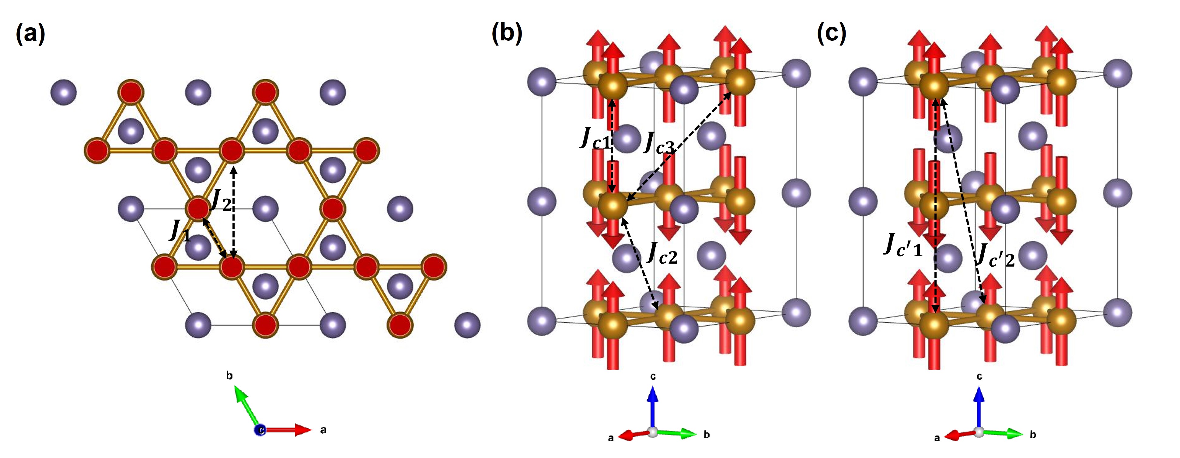
Figure 1: Crystal and magnetic structures of FeGe. Yellow and purple spheres represent Fe and Ge atoms respectively, while arrows denote magnetic moments of Fe atoms. (a) Top view of FeGe. The exchange interactions $J_{i}\$denote the $i$th-nearest-neighbor interactions between Fe ions within kagome layers. (b) The exchange interactions $J_{ci}$ denote the $i$th-nearest-neighbor interactions between Fe ions on the nearest kagome layers. (c) The exchange interactions $J_{c^{\prime}i}$ denote the $i$th-nearest-neighbor interactions between Fe ions on the next nearest kagome layers.

II Method

The first-principles calculations have been carried out by using the full potential linearized augmented plane-wave method as implemented in the Wien2k package Blaha et al. (2001). The converged k-point Monkhorst-Pack meshes are used for the calculations depending on materials. The self-consistent calculations are considered to be converged when the difference in the total energy of the crystal does not exceed $0.01mRy$. We adopt local spin-density approximation (LSDA) Vosko et al. (1980) as the exchange-correlation potential, and include the spin orbit coupling (SOC) using the second-order variational procedure Koelling and Harmon (1977).

The spin exchange interactions, including Heisenberg and DM interactions Dzyaloshinsky (1958); Moriya (1960), are calculated using first principles based on combining magnetic force theorem and linear-response approach Liechtenstein et al. (1987); Wan et al. (2006, 2009), which have successfully applied to various magnetic materials Wan et al. (2006, 2009, 2011, 2021); Wang et al. (2019).

Monte Carlo (MC) simulations are performed with Metropolis algorithm for Heisenberg model Metropolis and Ulam (1949); Shen et al. (2022); Cao et al. (2009). The size of the cell in the MC simulation are 16$\times$16$\times$16-unit cells with periodic boundary conditions. At each temperature we carry out 400000 sweeps to prepare the system, and sample averages are accumulated over 800000 sweeps.

III Results

III.1 The electronic and magnetic properties

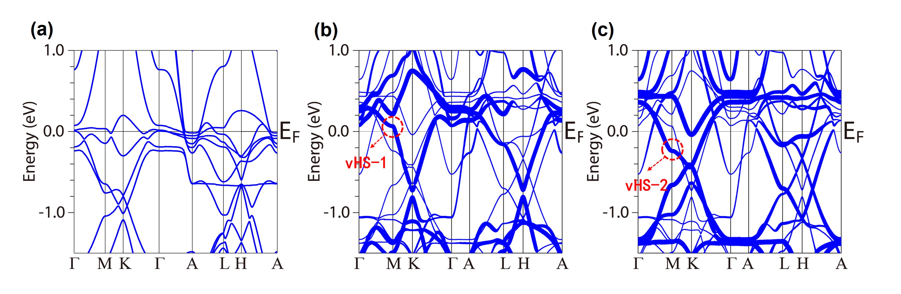
Figure 2: (a) Band structure of nonmagnetic FeGe from LDA + SOC calculation. (b),(c) Orbital-resolved band structure of Fe-$d_{xy}/d_{x^{2}-y^{2}}$ and Fe-$d_{xz}/d_{yz}$ for A-type AFM configuration with spin orientations along the (001) direction from LSDA + SOC calculation.

The pristine phase of FeGe crystallizes in the hexagonal structure with space group P6/mmm (No. 191) Ohoyama et al. (1963), where the coordinates of the atoms are shown in table 2 and Fig. 1. Firstly we perform nonmagnetic local-density approximation (LDA) + SOC calculation, and show the band structures in Fig. 2(a). While Ge-2$p$ states are mainly located between -6.0 and -2.0 eV, the main contribution around the Fermi level comes from the 3$d$ orbitals of Fe ions, as shown in Fig. 4 of Appendix. Consistent with previous first-principle calculations Setty et al. (2022); Teng et al. (2022a), the kagome flat bands around the Fermi level exhibit a large peak in the density of states, which indicates the magnetic instability. Therefore, LSDA + SOC calculations are performed based on the A-type AFM configuration and the band structures are shown in Figs. 2(b) and 2(c). The magnetic moment of Fe ions is estimated to be 1.55 $\mu_{B}$, which is in agreement with the previous experimental value around 1.7 $\mu_{B}$ Häggström et al. (1975); Forsyth et al. (1978). Note that each kagome layer is FM and the key signatures of electronic structures in kagome lattice are remained. The magnetic splitting is around 1.8 eV (see Fig. 4 of Appendix), which makes that the flat bands above and below Fermi level correspond to the spin minority bands and spin majority bands respectively. Meanwhile, the vHSs that are relatively far from the Fermi level in the nonmagnetic state, are brought near the Fermi level by the spin splitting, as shown in Figs. 2(b) and 2(c). We present orbital-resolved band structures, and find that the vHSs near the Fermi level, which marked as vHS-1 and vHS-2 in Figs. 2(b) and 2(c), are mainly contributed by the $d_{xy}/d_{x^{2}-y^{2}}$ and $d_{xz}/d_{yz}$ orbitals respectively. These vHSs near the Fermi level are suggested to induce symmetry-breaking CDW order in kagome metal FeGe Teng et al. (2022a).

Table 1: Spin exchange parameters (in meV) including Heisenberg and DM interactions of FeGe evaluated from LSDA+SOC calculations, respectively. The Fe-Fe distances and the corresponding number of neighbors NN are presented in the second and third columns.

	Distance($\mathring{\mathrm{A}}$)	NN	J	DM
$J_{1}$	2.50	4	-41.97	(0, 0, 0.03)
$J_{2}$	4.33	4	5.49	(0, 0, -0.12)
$J_{c1}$	4.05	2	8.44	(0, 0, 0)
$J_{c2}$	4.76	8	-2.04	(0.01, -0.02, -0.07)
$J_{c3}$	5.93	8	1.81	(0.07, -0.04, -0.09)
$J_{c^{\prime}1}$	8.11	2	-0.66	(0, 0, 0)
$J_{c^{\prime}2}$	8.49	8	0.09	(-0.04, -0.09, -0.03)

To quantitatively understand the rich magnetic phenomenon in kagome FeGe, a microscopic magnetic model with proper parameters is extremely important. Based on the calculated electronic structures, we estimate the exchange parameters including Heisenberg and DM interactions using the linear-response approach Liechtenstein et al. (1987); Wan et al. (2006, 2009) and summarize the results in table 1. As shown in Fig. 1, we divide the magnetic interactions considered into three types: the exchange interactions $J_{i}$, $J_{ci}$ and $J_{c^{\prime}i}\$represent the $i$th-nearest-neighbor interactions between Fe ions within kagome layers, on the nearest kagome layers, and on the next nearest kagome layers respectively. As shown in table 1, the in-plane nearest neighbor coupling $J_{1}$ favors FM order and is estimated to be -41.97 meV, which has the similar value with the one in kagome FeSn (around -50 meV) Xie et al. (2021); Sales et al. (2019); Do et al. (2022); Zhang et al. (2022). Note that the distance in $J_{1}$ is 2.5 Å while the others are all greater than 4 Å. Though there are also AFM in-plane magnetic interactions such as in-plane next-nearest neighbor coupling $J_{2}$, they are at least an order of magnitude smaller than $J_{1}$, resulting in each FM kagome layer. As the out-of-plane nearest neighbor coupling, $J_{c1}$ is estimated to be 8.44 meV. It makes the magnetic moments stacked antiferromagnetically between kagome layers, consequently resulting in the A-type AFM order in kagome FeGe, which is consistent with the experiment Beckman et al. (1972). It is worth mentioning that, SOC always exists and leads to the DM interactions even in the centrosymmetric compound FeGe, since not all Fe-Fe bonds have inversion symmetry. For the equivalent DM interactions connected by the crystal symmetry (see table 3-5 in Appendix), we only present one of them as a representative. As shown in table 1, the in-plane nearest neighbor $\mathbf{D}_{1}$ has the form of (0, 0, $D_{1}^{z}$) according to the crystal symmetry, and $D_{1}^{z}$ is estimated to be 0.03 meV. Meanwhile, the in-plane next nearest neighbor $\mathbf{D}_{2}$ is estimated to be (0, 0, $-$0.12) meV. For the out-of-plane nearest neighbor, $\mathbf{D}_{c1}$ is zero because its bond has an inversion center. The other calculated DM interactions are also listed in table 1, and most of them are small in the order of 0.01 meV.

To explore the magnetic anisotropy in kagome FeGe, we consider the MAE with the expression $E_{MAE}=K_{2}\sin^{2}\theta+K_{4}\sin^{4}\theta$ Beckman et al. (1972); Forsyth et al. (1978); Bernhard et al. (1984, 1988) neglecting terms of order higher than four, where $\theta$ is the angle between the magnetic moment and the z-axis. The values of $K_{2}$ and $K_{4}$ are estimated to be 0.066 meV and 0.018 meV respectively based on the approach of Ref. Mackintosh and Andersen (1980); Weinert et al. (1985), which are in reasonable agreement with the experimental values 0.021 meV Bernhard et al. (1988) and 0.012 meV Beckman et al. (1972). Here $K_{2}$ and $K_{4}$ are both positive, making out-of-plane magnetization favored, which is different from the easy-plane anisotropy in FeSn Sales et al. (2019). Note that positive $K_{4}$ is the requirement for the stability of the double cone magnetic structure, which will be discussed below.

According to the experiments Beckman et al. (1972), the Curie-Weiss temperature $\theta_{CW}$ in kagome FeGe is -200 K while the Néel temperature $T_{N}$ is 410 K. The relative low value of the frustration index $|\theta_{CW}|$/$T_{N}$ (smaller than 1) reveals the interplay of the FM and AFM interactions Baral et al. (2017). As shown in table 1, our calculated results of spin exchange couplings also verify the coexistence of the FM and AFM interactions. Based on these calculated spin exchange parameters, we calculate Néel temperature and Curie-Weiss temperature by MC simulations Metropolis and Ulam (1949); Shen et al. (2022); Cao et al. (2009). The $\theta_{CW}$ and$\ T_{N}$ are calculated to be -219 K and 370 K respectively, which agrees well with the experiment Beckman et al. (1972).

Similar to the electronic structure of a kagome lattice, the spin wave for a localized spin model with FM nearest-neighbor magnetic exchange also yields a flat magnetic band and a Dirac magnon Chisnell et al. (2015). Using the calculated spin model parameters, one can obtain the magnon spectrum Holstein and Primakoff (1940); Wang et al. (2021). The calculated spin-wave dispersion along the high-symmetry axis is shown in Fig. 3, which basically captures the key features of kagome lattice geometry. Similar with FeSn case Xie et al. (2021); Sales et al. (2019); Do et al. (2022); Zhang et al. (2022), strongly dispersive magnons in the xy-plane extend to about 260 meV, where the magnon dispersion along the out-of-plane direction has relatively small bandwidth of less than 15 meV, reflecting the quasi-two-dimensional magnetic properties in kagome FeGe. Meanwhile, the Dirac-like node appears at the K point at about 107 meV, and we find that DM interactions introduce a gap around 1 meV at the Dirac point, as shown in the inset of Fig. 3. Furthermore, the single-ion anisotropy produces a spin gap of about 2 meV, which could be verified in future inelastic neutron scattering experiments.

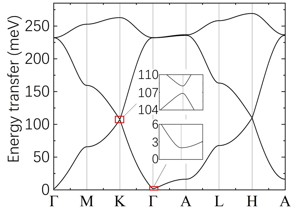
Figure 3: Calculated spin-wave dispersion curves along the high-symmetry axis for FeGe. The insets show the spin gap at $\Gamma$ point induced by easy-axis anisotropy, and the gap located at about 107 meV of K point induced by DM interactions.

III.2 The double cone magnetic structure

Table 2: Four types of $2\times 2\times 2$ CDW phases which can lead to non-zero DM contribution to double cone spin structure. The corresponding Wyckoff positions and the coordinates of the atoms in the pristine phase and these four CDW phases are summarized.

Pristine phase(P6/mmm)			$P622$(type I)			$P622$(type II)			$P6$3$22$(type I)			$P6$3$22$(type II)
	WP	Coordinates		WP	Coordinates		WP	Coordinates		WP	Coordinates		WP	Coordinates
Ge1	1a	(0, 0, 0)	Ge1	1a	(0, 0, 0)	Ge1	2e	(0, 0, z1)	Ge1	2a	(0, 0, 0)	Ge1	2b	(0, 0, 1/4)
			Ge2	1b	(0, 0, 1/2)	Ge2	6i	(1/2, 0, z2)	Ge2	6g	(x1, 0, 0)	Ge2	6h	(x1, 2x1, 1/4)
			Ge3	3f	(0, 1/2, 0)
			Ge4	3g	(0, 1/2, 1/2)
Ge2	2d	(1/3, 2/3, 1/2)	Ge5	4h	(1/3, 2/3, z1)	Ge3	2c	(1/3, 2/3, 0)	Ge3	2c	(1/3, 2/3, 1/4)	Ge3	4f	(1/3, 2/3, z2)
			Ge6	12n	(x2, y2, z2)	Ge4	2d	(1/3, 2/3,1/2)	Ge4	2d	(1/3, 2/3, 3/4)	Ge4	12i	(x3, y3, z3)
						Ge5	6l	(x3, 2x3, 0)	Ge5	6h	(x2, 2x2, 1/4)
						Ge6	6m	(x4, 2x4, 1/2)	Ge6	6h	(x3, 2x3, 1/4)
Fe	3f	(1/2, 0, 0)	Fe1	6j	(x3, 0, 0)	Fe1	12n	(x5, y5, z5)	Fe1	6g	(x4, 0, 0)	Fe1	6h	(x4, 2x4, 1/4)
			Fe2	6k	(x4, 0, 1/2)	Fe2	12n	(x6, y6, z6)	Fe2	6g	(x5, 0, 0)	Fe2	6h	(x5, 2x5, 1/4)
			Fe3	6l	(x5, 2x5, 0)				Fe3	12i	(x6, y6, z6)	Fe3	12i	(x6, y6, z6)
			Fe4	6m	(x6, 2x6, 1/2)

At $T_{canting}$ = 60 K, the kagome lattice FeGe becomes a c-axis double cone AFM structure Beckman et al. (1972); Häggström et al. (1975); Forsyth et al. (1978); Bernhard et al. (1984, 1988) where the magnetic ground state could be written as Eq. (10) in Appendix. Considering the magnetic interactions and the MAE, the total energy of the double cone spin structure could be written as Eq. (12) in Appendix. When DM interactions are not considered, the extremum condition of the total energy gives the equilibrium value of wave vector $\delta$ and the cone half angle $\theta$ (i.e. Eq. (13) and (14) in Appendix)

$$\cos\delta = \frac{\sum_{i}N_{ci}J_{ci}}{4\sum_{i}N_{c^{\prime}i}J_{c^{\prime}i}}$$ (1)

$$\sin^{2}\theta = -\frac{K_{2}-\frac{1}{2N}\sum_{i}N_{c^{\prime}i}J_{c^{\prime}i}\delta^{4}}{2K_{4}}$$ (2)

Note that the minimum of the total energy requires that the second derivative of Eq. (12) in Appendix is positive, thus $K_{4}$ must be positive. Hence $K_{2}-\frac{1}{2N}\sum_{i}N_{c^{\prime}i}J_{c^{\prime}i}\delta^{4}$ (i.e. the numerator of Eq. (2)) must be negative. However, our reasonable magnetic parameters cannot explain the double cone magnetic ground state. The value of wave vector $\delta$ is small in experimental measurement (0.17 in Ref. Beckman et al. (1972) and 0.25 in Ref. Gäfvert et al. (1977)), thus $\delta^{4}$ is around 0.001. Meanwhile, the value of $\frac{1}{2N}\sum_{i}N_{c^{\prime}i}J_{c^{\prime}i}$ is of the order of 1 meV, which obviously cannot explain the double cone magnetic structure Beckman et al. (1972).

We thus consider the effect of DM interactions on double cone spin structure. Since the exchange interactions between two next nearest neighbor kagome layers are relatively small, we only consider the Heisenberg and DM interactions between two nearest neighbor kagome layers, i.e. $J_{ci}$ and $\mathbf{D}_{ci}$. We find that wave vector $\delta$ and the cone half angle $\theta$ have the expressions as (i.e. Eq. (15) and (16) in Appendix)

$$\tan\delta = \frac{\sum_{i,j}D_{ci,j}^{z}}{\sum_{i}N_{ci}J_{ci}}$$ (3)

$$\sin^{2}\theta = -\frac{K_{2}-\frac{1}{2N}\sum_{i,j}D_{ci,j}^{z}\delta}{2K_{4}}$$ (4)

It should be noted that, comparing Eq. (2) and (4), DM interactions are more efficient than Heisenberg interactions for causing double cone spin structure since $\delta$ is small. Though the space group $P6/mmm$ of high-temperature phase in FeGe has a global inversion center, not all Fe-Fe bonds have inversion symmetry and DM interactions could exist. However, according to the inversion symmetry of space group $P6/mmm$, the total contribution of DM interactions to the energy of double cone magnetic structure in Eq. (12) is absent, i.e. $\sum_{i,j}D_{ci,j}^{z}=0$ (see Appendix D). Meanwhile, mirror symmetries in space group $P6/mmm$ would also eliminate the contribution of DM interactions based on the symmetry analysis. Therefore, DM interactions have no net contribution to double cone magnetic structure with the symmetry of high-temperature phase. For the CDW phases with the space group of $P6/mmm$ suggested by Ref. Shao et al. (2022); Miao et al. (2022) (the first two structures of the table 6 in Appendix), the total contribution of DM interactions is still absent and cannot explain the magnetic ground state of double cone spin structure.

III.3 The interplay of CDW and double cone structure

As mentioned above, DM interactions play a more important role in the double cone spin structure. Meanwhile, it is very sensitive to atomic displacements. Therefore, in the following we explore the CDW phases with symmetry-allowed DM contribution to double cone spin structure which may explain the canted magnetic ground state.

The $2\times 2\times 2$ supercell structure of CDW phase (compared with the nonmagnetic pristine phase) is suggested experimentally Teng et al. (2022b); Yin et al. (2022); Shao et al. (2022); Miao et al. (2022). Considering all CDW phases whose associated point group in the maximal subgroups of $D_{6h}$, we find 68 different possible CDW phases which are the subgroups of the parent $P6/mmm$ phase with $2\times 2\times 2$ supercell (see details in Appendix D). The corresponding relations of atomic positions between the pristine phase and these proposed CDW phases are all summarized in table 6-10 of Appendix.

Note that the inversion symmetry and mirror symmetries would all eliminate the net contribution of DM interactions as disscussed above. We find that among these 68 proposed CDW phases, only four distorted structures break all these symetries above, and can lead to non-zero DM contribution in Eq. (12) of Appendix. We list the corresponding Wyckoff positions (WP) and the coordinates of the atoms in the pristine phase and these four CDW phases in table 2. They comes from two space groups $P622$ and $P6_{3}22$. It should be mentioned that there are two different CDW phases for each of these two space groups, which are labeled as (type I) and (type II) in table 2. Note that the CDW phase with $P622$ space group is also suggested in Ref. Teng et al. (2022b).

Raman spectroscopy is a fast and usually non-destructive technique which can be used to characterize the structural distortion of materials. Based on the atomic coordinates in table 2, we predict the irreducible representation of the Raman active modes of these four proposed CDW phases using symmetry analysis Bradley and Cracknell (1972). For $P622$ (type I) and (type II) CDW phases, the Raman active modes are 8$\mathrm{{A_{1}}}$ + 26$\mathrm{{E_{1}}}$ + 22$\mathrm{{E_{2}}}$ and 10$\mathrm{{A_{1}}}$ + 26$\mathrm{{E_{1}}}$ + 22$\mathrm{{E_{2}}}$. Meanwhile, for $P6_{3}22$ (type I) and (type II), the Raman active modes are 8$\mathrm{{A_{1}}}$ + 24$\mathrm{{E_{1}}}$ + 24$\mathrm{{E_{2}}}$ and 10$\mathrm{{A_{1}}}$ + 24$\mathrm{{E_{1}}}$ + 24$\mathrm{{E_{2}}}$, respectively. Note that even within the same symmetry of space group $P622$, the different structural distortion of CDW phases $P622$ (type I) and (type II) could result in the different number of Raman active modes (56 and 58 respectively), which could be identified by Raman spectroscopy.

IV CONCLUSION

In conclusion, we systematically analyze the electronic and magnetic properties of kagome FeGe. Our numerical results show that this material is a magnetic metal exhibiting large magnetic splitting around 1.8 eV. The magnetic splitting makes the flat bands away from Fermi level, and bring two vHSs near the Fermi level. We estimate the magnetic parameters, and find that the ferromagnetic nearest-neighbor $J_{1}$ dominates over the others, while the magnetic interactions between nearest kagome layers favors antiferromagnetic. Based on these spin exchange parameters, the calculated Néel temperature and Curie-Weiss temperature also agree well with the experiments. Furthermore, the magnetic excitation spectra are calculated using linear spin wave theory and a spin gap about 2 meV is predicted. Note that the double cone magnetic transition at a lower temperature cannot be reproduced by these reasonable magnetic parameters. Meanwhile, due to the inversion symmetry and mirror symmetries in the space group $P6/mmm$ of high-temperature phase, the total contribution of DM interactions to the double cone magnetic structure is absent. Since DM interactions are very sensitive to small atomic displacements and symmetry restrictions, and also much more efficient than Heisenberg interactions for causing this canted spin structure, we propose that the double cone spin structure may arise from the structural distortion. We explore 68 possible CDW phases of kagome FeGe which are subgroups of the pristine phase with $2\times 2\times 2$ supercell, and symmetry-allowed four CDW structures which have non-zero DM contribution and may result in double cone spin structure are proposed. These four CDW phases belong to two space groups $P622$ and $P6_{3}22$, and we further propose that they can be identified from their different numbers of Raman active peaks. Therefore, we believe that symmetry analysis plays an important role in exploring the possible structural distortion in complex magnetic configurations.

V Acknowledgements

This work was supported by the NSFC (No. 12188101, 11834006, 12004170, 11790311, 51721001), National Key R&D Program of China (No. 2018YFA0305704), Natural Science Foundation of Jiangsu Province, China (Grant No. BK20200326), and the excellent programme in Nanjing University. Xiangang Wan also acknowledges the support from the Tencent Foundation through the XPLORER PRIZE.

VI Appendix

VI.1 The density of states in kagome FeGe

The Partial density of states (DOS) of FeGe from LSDA + SOC calculations are shown in Fig. 4.

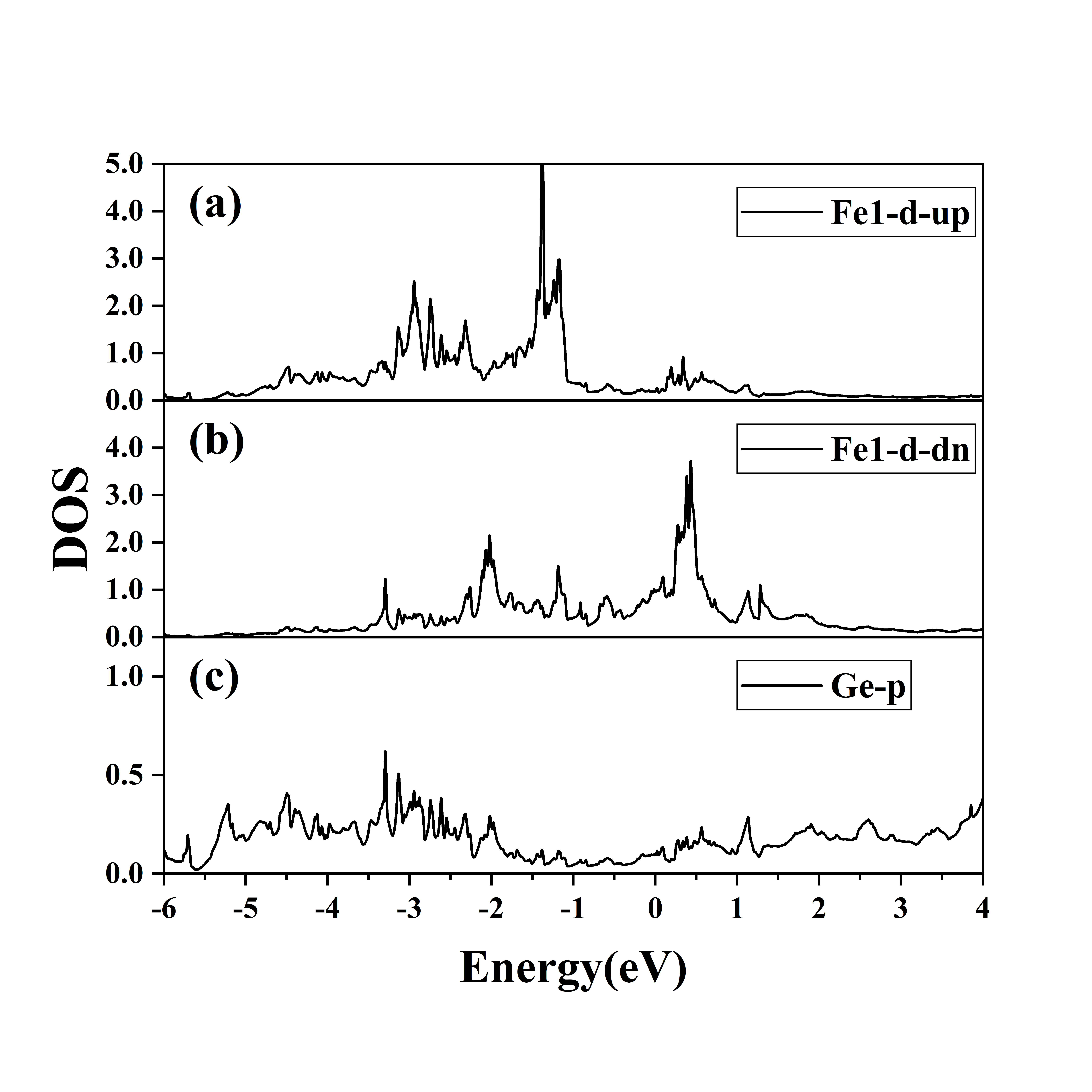
Figure 4: Partial DOS of FeGe from LSDA + SOC calculations. The Fermi energy is set to zero. (a) and (b) represent the spin-up and spin-down channel of $d$ orbitals in Fe1 atom located at (1/2,0,0), while (c) represents the DOS of Ge-$p$ orbitals.

VI.2 The symmetry restrictions on the magnetic interactions

Table 3: The distances, the bond information and the symmetry restricted interactions of corresponding Fe ions within xy-planes. Here $n$, $n^{\prime}$ and $R_{l}$ correspond to $\mathbf{J}_{\boldsymbol{\tau}_{n},\boldsymbol{\tau_{n^{\prime}}+}\mathbf{R}_{l}}$, where $R_{l}$ and $\tau_{n}$ represent the lattice translation vector and the position of magnetic ions in the lattice basis. Three magnetic ions are located at $\tau_{1}$ (1/2, 0, 0), $\tau_{2}$ (0, 1/2, 0), and $\tau_{3}$ (1/2, 1/2, 0). The equivalent $\mathbf{D}_{i}$’s are labeled as the sub-index of $j$, i.e. the $\mathbf{D}_{i,j}$ in the table.

Distance($\mathring{\mathrm{A}}$)	$n$	$n^{\prime}$	$R_{l}$	$J$	DM
2.50	3	1	(0,1,0)	$J_{1}$	$\mathbf{D}_{1,1}(0,0,D_{1}^{z})$
	1	2	(0,-1,0)	$J_{1}$	$\mathbf{D}_{1,2}(0,0,D_{1}^{z})$
	2	3	(0,0,0)	$J_{1}$	$\mathbf{D}_{1,3}(0,0,D_{1}^{z})$
	3	1	(0,0,0)	$J_{1}$	$\mathbf{D}_{1,4}(0,0,D_{1}^{z})$
	1	2	(1,0,0)	$J_{1}$	$\mathbf{D}_{1,5}(0,0,D_{1}^{z})$
	2	3	(-1,0,0)	$J_{1}$	$\mathbf{D}_{1,6}(0,0,D_{1}^{z})$
4.33	1	2	(1,-1,0)	$J_{2}$	$\mathbf{D}_{2,1}(0,0,D_{2}^{z})$
	2	3	(0,1,0)	$J_{2}$	$\mathbf{D}_{2,2}(0,0,D_{2}^{z})$
	3	1	(-1,0,0)	$J_{2}$	$\mathbf{D}_{2,3}(0,0,D_{2}^{z})$
	1	2	(0,0,0)	$J_{2}$	$\mathbf{D}_{2,4}(0,0,D_{2}^{z})$
	2	3	(-1,-1,0)	$J_{2}$	$\mathbf{D}_{2,5}(0,0,D_{2}^{z})$
	3	1	(1,1,0)	$J_{2}$	$\mathbf{D}_{2,6}(0,0,D_{2}^{z})$

Table 4: The distances, the bond information and the symmetry restricted interactions of corresponding Fe ions between nearest-neighbor $(001)$-planes. Here $n$, $n^{\prime}$ and $R_{l}$ correspond to $\mathbf{J}_{\boldsymbol{\tau}_{n},\boldsymbol{\tau_{n^{\prime}}+}\mathbf{R}_{l}}$, where $R_{l}$ and $\tau_{n}$ represent the lattice translation vector and the position of magnetic ions in the lattice basis. Three magnetic ions are located at $\tau_{1}$ (1/2, 0, 0), $\tau_{2}$ (0, 1/2, 0), and $\tau_{3}$ (1/2, 1/2, 0). The equivalent $\mathbf{D}_{ci}$’s are labeled as the sub-index of $j$, i.e. the $\mathbf{D}_{ci,j}$ in the table.

Distance($\mathring{\mathrm{A}}$)	$n$	$n^{\prime}$	$R_{l}$	$J$	DM
4.05	1	1	(0,0,1)	$J_{c1}$	$\mathbf{D}_{c1,1}(0,0,0)$
	2	2	(0,0,1)	$J_{c1}$	$\mathbf{D}_{c1,2}(0,0,0)$
	3	3	(0,0,1)	$J_{c1}$	$\mathbf{D}_{c1,3}(0,0,0)$
4.76	3	1	(0,0,1)	$J_{c2}$	$\mathbf{D}_{c2,1}(D_{c2}^{x},-\sqrt{3}D_{c2}^{x},D_{c2}^{z})$
	1	2	(1,0,1)	$J_{c2}$	$\mathbf{D}_{c2,2}(D_{c2}^{x},\sqrt{3}D_{c2}^{x},D_{c2}^{z})$
	2	3	(-1,0,1)	$J_{c2}$	$\mathbf{D}_{c2,3}(-2D_{c2}^{x},0,D_{c2}^{z})$
	3	1	(0,1,1)	$J_{c2}$	$\mathbf{D}_{c2,4}(-D_{c2}^{x},\sqrt{3}D_{c2}^{x},D_{c2}^{z})$
	1	2	(0,-1,1)	$J_{c2}$	$\mathbf{D}_{c2,5}(-D_{c2}^{x},-\sqrt{3}D_{c2}^{x},D_{c2}^{z})$
	2	3	(0,0,1)	$J_{c2}$	$\mathbf{D}_{c2,6}(2D_{c2}^{x},0,D_{c2}^{z})$
	1	3	(0,-1,1)	$J_{c2}$	$\mathbf{D}_{c2,7}(-D_{c2}^{x},\sqrt{3}D_{c2}^{x},-D_{c2}^{z})$
	2	1	(0,1,1)	$J_{c2}$	$\mathbf{D}_{c2,8}(-D_{c2}^{x},-\sqrt{3}D_{c2}^{x},-D_{c2}^{z})$
	3	2	(0,0,1)	$J_{c2}$	$\mathbf{D}_{c2,9}(2D_{c2}^{x},0,-D_{c2}^{z})$
	1	3	(0,0,1)	$J_{c2}$	$\mathbf{D}_{c2,10}(D_{c2}^{x},-\sqrt{3}D_{c2}^{x},-D_{c2}^{z})$
	2	1	(-1,0,1)	$J_{c2}$	$\mathbf{D}_{c2,11}(D_{c2}^{x},\sqrt{3}D_{c2}^{x},-D_{c2}^{z})$
	3	2	(1,0,1)	$J_{c2}$	$\mathbf{D}_{c2,12}(-2D_{c2}^{x},0,-D_{c2}^{z})$
5.93	2	1	(-1,1,1)	$J_{c3}$	$\mathbf{D}_{c3,1}(-\sqrt{3}D_{c3}^{y},D_{c3}^{y},-D_{c3}^{z})$
	3	2	(0,-1,1)	$J_{c3}$	$\mathbf{D}_{c3,2}(0,-2D_{c3}^{y},-D_{c3}^{z})$
	1	3	(1,0,1)	$J_{c3}$	$\mathbf{D}_{c3,3}(\sqrt{3}D_{c3}^{y},D_{c3}^{y},-D_{c3}^{z})$
	2	1	(0,0,1)	$J_{c3}$	$\mathbf{D}_{c3,4}(\sqrt{3}D_{c3}^{y},-D_{c3}^{y},-D_{c3}^{z})$
	3	2	(1,1,1)	$J_{c3}$	$\mathbf{D}_{c3,5}(0,2D_{c3}^{y},-D_{c3}^{z})$
	1	3	(-1,-1,1)	$J_{c3}$	$\mathbf{D}_{c3,6}(-\sqrt{3}D_{c3}^{y},-D_{c3}^{y},-D_{c3}^{z})$
	1	2	(0,0,1)	$J_{c3}$	$\mathbf{D}_{c3,7}(\sqrt{3}D_{c3}^{y},-D_{c3}^{y},D_{c3}^{z})$
	2	3	(-1,-1,1)	$J_{c3}$	$\mathbf{D}_{c3,8}(0,2D_{c3}^{y},D_{c3}^{z})$
	3	1	(1,1,1)	$J_{c3}$	$\mathbf{D}_{c3,9}(-\sqrt{3}D_{c3}^{y},-D_{c3}^{y},D_{c3}^{z})$
	1	2	(1,-1,1)	$J_{c3}$	$\mathbf{D}_{c3,10}(-\sqrt{3}D_{c3}^{y},D_{c3}^{y},D_{c3}^{z})$
	2	3	(0,1,1)	$J_{c3}$	$\mathbf{D}_{c3,11}(0,-2D_{c3}^{y},D_{c3}^{z})$
	3	1	(-1,0,1)	$J_{c3}$	$\mathbf{D}_{c3,12}(\sqrt{3}D_{c3}^{y},D_{c3}^{y},D_{c3}^{z})$

Table 5: The distances, the bond information and the symmetry restricted interactions of corresponding Fe ions between next-nearest-neighbor $(001)$-planes. Here $n$, $n^{\prime}$ and $R_{l}$ correspond to $\mathbf{J}_{\boldsymbol{\tau}_{n},\boldsymbol{\tau_{n^{\prime}}+}\mathbf{R}_{l}}$, where $R_{l}$ and $\tau_{n}$ represent the lattice translation vector and the position of magnetic ions in the lattice basis. Three magnetic ions are located at $\tau_{1}$ (1/2, 0, 0), $\tau_{2}$ (0, 1/2, 0), and $\tau_{3}$ (1/2, 1/2, 0). The equivalent $\mathbf{D}_{c^{\prime}i}$’s are labeled as the sub-index of $j$, i.e. the $\mathbf{D}_{c^{\prime}i,j}$ in the table.

Distance($\mathring{\mathrm{A}}$)	$n$	$n^{\prime}$	$R_{l}$	$J$	DM
8.11	1	1	(0,0,2)	$J_{c^{\prime}1}$	$\mathbf{D}_{c^{\prime}1,1}(0,0,0)$
	2	2	(0,0,2)	$J_{c^{\prime}1}$	$\mathbf{D}_{c^{\prime}1,2}(0,0,0)$
	3	3	(0,0,2)	$J_{c^{\prime}1}$	$\mathbf{D}_{c^{\prime}1,3}(0,0,0)$
8.49	2	1	(0,1,2)	$J_{c^{\prime}2}$	$\mathbf{D}_{c^{\prime}2,1}(D_{c^{\prime}2}^{x},\sqrt{3}D_{c^{\prime}2}^{x},D_{c^{\prime}2}^{z})$
	3	2	(0,0,2)	$J_{c^{\prime}2}$	$\mathbf{D}_{c^{\prime}2,2}(-2D_{c^{\prime}2}^{x},0,D_{c^{\prime}2}^{z})$
	1	3	(0,-1,2)	$J_{c^{\prime}2}$	$\mathbf{D}_{c^{\prime}2,3}(D_{c^{\prime}2}^{x},-\sqrt{3}D_{c^{\prime}2}^{x},D_{c^{\prime}2}^{z})$
	2	1	(-1,0,2)	$J_{c^{\prime}2}$	$\mathbf{D}_{c^{\prime}2,4}(-D_{c^{\prime}2}^{x},-\sqrt{3}D_{c^{\prime}2}^{x},D_{c^{\prime}2}^{z})$
	3	2	(1,0,2)	$J_{c^{\prime}2}$	$\mathbf{D}_{c^{\prime}2,5}(2D_{c^{\prime}2}^{x},0,D_{c^{\prime}2}^{z})$
	1	3	(0,0,2)	$J_{c^{\prime}2}$	$\mathbf{D}_{c^{\prime}2,6}(-D_{c^{\prime}2}^{x},\sqrt{3}D_{c^{\prime}2}^{x},D_{c^{\prime}2}^{z})$
	1	2	(1,0,2)	$J_{c^{\prime}2}$	$\mathbf{D}_{c^{\prime}2,7}(-D_{c^{\prime}2}^{x},-\sqrt{3}D_{c^{\prime}2}^{x},-D_{c^{\prime}2}^{z})$
	2	3	(-1,0,2)	$J_{c^{\prime}2}$	$\mathbf{D}_{c^{\prime}2,8}(2D_{c^{\prime}2}^{x},0,-D_{c^{\prime}2}^{z})$
	3	1	(0,0,2)	$J_{c^{\prime}2}$	$\mathbf{D}_{c^{\prime}2,9}(-D_{c^{\prime}2}^{x},\sqrt{3}D_{c^{\prime}2}^{x},-D_{c^{\prime}2}^{z})$
	1	2	(0,-1,2)	$J_{c^{\prime}2}$	$\mathbf{D}_{c^{\prime}2,10}(D_{c^{\prime}2}^{x},\sqrt{3}D_{c^{\prime}2}^{x},-D_{c^{\prime}2}^{z})$
	2	3	(0,0,2)	$J_{c^{\prime}2}$	$\mathbf{D}_{c^{\prime}2,11}(-2D_{c^{\prime}2}^{x},0,-D_{c^{\prime}2}^{z})$
	3	1	(0,1,2)	$J_{c^{\prime}2}$	$\mathbf{D}_{c^{\prime}2,12}(D_{c^{\prime}2}^{x},-\sqrt{3}D_{c^{\prime}2}^{x},-D_{c^{\prime}2}^{z})$

Here we consider a general pairwise spin model

$$H=\sum_{l,n,l^{\prime},n^{\prime}}\mathbf{S}_{ln}\mathbf{J}_{\mathbf{R}_{l}+\boldsymbol{\tau}_{n},\mathbf{R}_{l^{\prime}}+\boldsymbol{\tau_{n^{\prime}}}}\mathbf{S}_{l^{\prime}n^{\prime}}$$ (5)

where $\mathbf{J}_{\mathbf{R}_{l}+\boldsymbol{\tau}_{n},\mathbf{R}_{l^{\prime}}+\boldsymbol{\tau_{n^{\prime}}}}$, a $3\times 3$ tensor, represents the spin exchange parameters. $\mathbf{R}_{l}$ and $\boldsymbol{\tau}_{n}$ represent the lattice translation vector and the position of magnetic ions in the lattice basis, and $\mathbf{S}_{ln}$ means the spin at the site of $\mathbf{R}_{l}+\boldsymbol{\tau}_{n}.$Translation symmetry will restrict $\mathbf{J}_{\mathbf{R}_{l}+\boldsymbol{\tau}_{n},\mathbf{R}_{l^{\prime}}+\boldsymbol{\tau_{n^{\prime}}}}$ to be only related to $\mathbf{J}_{\boldsymbol{\tau}_{n},\boldsymbol{\tau_{n^{\prime}}+}\mathbf{R}_{l^{\prime\prime}}}$ where $R_{l^{\prime\prime}}=R_{l^{\prime}}-R_{l}$, irrespective of the starting unit cell. Other spatial symmetries will also give restrictions on the magnetic exchange interactions. We consider a general space group element $\{\alpha|\mathbf{t}\}$, where the left part represents the rotation and the right part means the lattice translation. Supposing under this symmetry operator, $\mathbf{R}_{m}+\boldsymbol{\tau}_{p}$ and $\mathbf{R}_{m^{\prime}}+\boldsymbol{\tau_{p^{\prime}}}$ transfer to $\mathbf{R}_{l}+\boldsymbol{\tau}_{n}$ and $\mathbf{R}_{l^{\prime}}+\boldsymbol{\tau_{n^{\prime}}}$, respectively, meanwhile the transformation of spin becomes $\mathbf{S}_{mp}=M(\alpha)\mathbf{S}_{ln}$, where $M(\alpha)$ is the representation matrix of the proper rotation part of the operation $\alpha$ in the coordinate system, we get the following expression:

$$H = \sum_{l,n,l^{\prime},n^{\prime}}\mathbf{S}_{ln}\mathbf{J}_{\mathbf{R}_{l}+\boldsymbol{\tau}_{n},\mathbf{R}_{l^{\prime}}+\boldsymbol{\tau_{n^{\prime}}}}\mathbf{S}_{l^{\prime}n^{\prime}}$$ (6)

$$= \sum_{l,n,l^{\prime},n^{\prime}}\mathbf{S}_{ln}M^{{\dagger}}(\alpha)M(\alpha)\mathbf{J}_{\mathbf{R}_{l}+\boldsymbol{\tau}_{n},\mathbf{R}_{l^{\prime}}+\boldsymbol{\tau_{n^{\prime}}}}M^{{\dagger}}(\alpha)M(\alpha)\mathbf{S}_{l^{\prime}n^{\prime}}$$

$$= \sum_{m,p,m^{\prime},p^{\prime}}\mathbf{S}_{mp}\left[M(\alpha)\mathbf{J}_{\mathbf{R}_{l}+\boldsymbol{\tau}_{n},\mathbf{R}_{l^{\prime}}+\boldsymbol{\tau_{n^{\prime}}}}M^{{\dagger}}(\alpha)\right]\mathbf{S}_{m^{\prime}p^{\prime}}$$

Then the exchange interactions should satisfy the following condition:

$$\mathbf{J}_{\mathbf{R}_{m}+\boldsymbol{\tau}_{p},\mathbf{R}_{m^{\prime}}+\boldsymbol{\tau_{p^{\prime}}}}=M(\alpha)\mathbf{J}_{\mathbf{R}_{l}+\boldsymbol{\tau}_{n},\mathbf{R}_{l^{\prime}}+\boldsymbol{\tau_{n^{\prime}}}}M^{{\dagger}}(\alpha)$$ (7)

After decomposing the $3\times 3$ tensor $\mathbf{J}$ into scalar Heisenberg term $J$ and vector DM term $\mathbf{D}$ as in the maintext, we obtain the following results:

$$J_{\mathbf{R}_{m}+\boldsymbol{\tau}_{p},\mathbf{R}_{m^{\prime}}+\boldsymbol{\tau_{p^{\prime}}}} = J_{\mathbf{R}_{l}+\boldsymbol{\tau}_{n},\mathbf{R}_{l^{\prime}}+\boldsymbol{\tau_{n^{\prime}}}}$$

$$\mathbf{D}_{\mathbf{R}_{m}+\boldsymbol{\tau}_{p},\mathbf{R}_{m^{\prime}}+\boldsymbol{\tau_{p^{\prime}}}} = M(\alpha)\mathbf{D}_{\mathbf{R}_{l}+\boldsymbol{\tau}_{n},\mathbf{R}_{l^{\prime}}+\boldsymbol{\tau_{n^{\prime}}}}$$ (8)

Meanwhile, it is should be noted that the Heisenberg and DM interactions obey the following commutation relations

$$J_{\mathbf{R}_{l^{\prime}}+\boldsymbol{\tau_{n^{\prime}},}\mathbf{R}_{l}+\boldsymbol{\tau}_{n}} = J_{\mathbf{R}_{l}+\boldsymbol{\tau}_{n},\mathbf{R}_{l^{\prime}}+\boldsymbol{\tau_{n^{\prime}}}}$$

$$\mathbf{D}_{\mathbf{R}_{l^{\prime}}+\boldsymbol{\tau_{n^{\prime}},}\mathbf{R}_{l}+\boldsymbol{\tau}_{n}} = -\mathbf{D}_{\mathbf{R}_{l}+\boldsymbol{\tau}_{n},\mathbf{R}_{l^{\prime}}+\boldsymbol{\tau_{n^{\prime}}}}$$ (9)

According to the above equations (i.e. Eq. (8) and (9)), one can obtain the symmetry restricted magnetic interactions for kagome FeGe with space group $P6/mmm$, as shown in table 3, 4 and 5. Note that the equivalent $\mathbf{D}_{i}$’s are labeled as the sub-index of $j$, i.e. the $\mathbf{D}_{i,j}$ in table 3, 4 and 5.

VI.3 The details of double cone structure

According to the experimental works Beckman et al. (1972); Forsyth et al. (1978); Bernhard et al. (1984, 1988), in hexagonal FeGe there is a transition from a uniaxial spin system to a double cone spin structure at $T_{canting}$ = 60 K Beckman et al. (1972), which is expressed by the following equations:

$$\left\langle S^{x}\right\rangle = S\sin\theta\cos\left(\left(\pi\pm\delta\right)\frac{z}{c}+\varphi\right)$$

$$\left\langle S^{y}\right\rangle = S\sin\theta\sin\left(\left(\pi\pm\delta\right)\frac{z}{c}+\varphi\right)$$

$$\left\langle S^{z}\right\rangle = S\cos\theta\cos\left(\frac{\pi z}{c}\right)$$ (10)

where $\theta$ is the cone half angle, and $c$ represents the lattice parameter. If $\delta=0$ there will be a simple tilting of the spins. When $\delta$ represents the small angle, Eq. (10) gives a double cone spin structure. Following the previous works Beckman et al. (1972); Forsyth et al. (1978); Bernhard et al. (1984, 1988), here we consider the MAE with the expression neglecting terms of order higher than four written as

$$E_{MAE}=K_{2}\sin^{2}\theta+K_{4}\sin^{4}\theta$$ (11)

Therefore the total energy of Eq. (5) and Eq. (11) in double cone spin structure per unit cell could be written as

$$E(\delta,\theta) = \sum_{i}N_{ci}J_{ci}(-\sin^{2}\theta\cos\delta-\cos^{2}\theta)$$ (12)

$$+\sum_{i}N_{c^{\prime}i}J_{c^{\prime}i}(\sin^{2}\theta\cos 2\delta+\cos^{2}\theta)$$

$$-\sum_{i,j}D_{ci,j}^{z}(\sin^{2}\theta\sin\delta)$$

$$-\sum_{i,j}D_{c^{\prime}i,j}^{z}(\sin^{2}\theta\sin 2\delta)$$

$$+N(K_{2}\sin^{2}\theta+K_{4}\sin^{4}\theta)$$

where $N_{ci}$ and $N_{c^{\prime}i}$ are the corresponding number of neighbors of $J_{ci}$ and $J_{c^{\prime}i}$, and $N$ represents the number of magnetic ions in one unit cell. When DM interactions are not considered, the extremum condition in total energ gives the equilibrium value of wave vector $\delta$ with following equation Beckman et al. (1972); Bernhard et al. (1988):

$$\cos\delta=\frac{\sum_{i}N_{ci}J_{ci}}{4\sum_{i}N_{c^{\prime}i}J_{c^{\prime}i}}$$ (13)

While the cone half angle $\theta$ has the expression as

$$\sin^{2}\theta=-\frac{K_{2}-\frac{1}{2N}\sum_{i}N_{c^{\prime}i}J_{c^{\prime}i}\delta^{4}}{2K_{4}}$$ (14)

A minimum in the total energy (see Eq. (12)) will occur only if $K_{4}$ is positive, and Eq. (14) requires that $K_{2}-\frac{1}{2N}\sum_{i}N_{c^{\prime}i}J_{c^{\prime}i}\delta^{4}$ must be negative.

When the magnetic interactions including Heisenberg and DM interactions between two nearest neighbor xy-planes, i.e. $J_{ci}$ and $\mathbf{D}_{ci}$, are considered, the equilibrium value of wave vector $\delta$ is obtained by the minimum in total energy written as

$$\tan\delta=\frac{\sum_{i,j}D_{ci,j}^{z}}{\sum_{i}N_{ci}J_{ci}}$$ (15)

where $j$ is the sub-index of the equivalent $\mathbf{D}_{ci}$’s. Meanwhile, we find the following expression for $\theta$

$$\sin^{2}\theta=-\frac{K_{2}-\frac{1}{2N}\sum_{i,j}D_{ci,j}^{z}\delta}{2K_{4}}$$ (16)

Note that in Eq. (16), DM interactions are combined with only the first order of $\delta$, and may have much more efficient than $J_{c^{\prime}i}$ in Eq. (14) since $\delta$ is small around 0.2 Beckman et al. (1972); Gäfvert et al. (1977). This implies that DM interactions may be the origin of double cone structure.

VI.4 The symmetry analysis of CDW phases

The high-temperature phase FeGe crystallizes in space group $P6/mmm$, which has the generators {3${}_{001}^{+}$$|$0}, {2₀₀₁$|$0}, {2₁₁₀$|$0} and {-1$|$0}, where the left part represents the rotation and the right part means the lattice translation (here -1 denotes the inversion symmetry). According to the inversion symmetry, the total contribution of DM interactions to the energy of double cone magnetic structure in Eq. (12) is absent, i.e. $\sum_{i,j}D_{ci,j}^{z}=0$, which is easy to see from the table 4-5. Firstly, each kagome layer is still FM in the double cone magnetic state, thus the in-plane DM interactions are ineffective. For interlayer DM interactions with an inversion center such as $\mathbf{D}_{c1}$, the inversion symmetry restricts it to be zero as shown in table 4. Meanwhile, for other interlayer DM interactions, the inversion symmetry combine the equivalent DM interactions in pairs. For example, as shown in table 4, the $\mathbf{D}_{c2,1}$ and $\mathbf{D}_{c2,7}$ are connected by the inversion symmetry, and have opposite values. Therefore, the summation over equivalent interlayer DM interactions are all zero due to the inversion symmetry. Note that not only inversion symmetry, but mirror symmetries such as {$m_{001}$$|$0}, {$m_{110}$$|$0}, {$m_{100}$$|$0}, {$m_{010}$$|$0}, {$m_{1-10}$$|$0}, {$m_{120}$$|$0} and {$m_{210}$$|$0} in space group $P6/mmm$, would also make the DM contribution to the canted magnetic ground state to be zero based on the similar analysis above. Therefore, DM interactions have no contribution to double cone magnetic structure with the symmetry of high-temperature phase.

As mentioned in the maintext, since the $2\times 2\times 2$ supercell structure of CDW phase (compared with the nonmagnetic pristine phase) is suggested experimentally Teng et al. (2022b); Yin et al. (2022); Shao et al. (2022); Miao et al. (2022), we present the possible CDW phases of kagome FeGe with $2\times 2\times 2$ supercell. The $2\times 2\times 2$ supercell without distortion has the symmetry of space group $P6/mmm$, the non-primitive translation operations $t_{x}$ {1$|$1/2,0,0}, $t_{y}$ {1$|$0,1/2,0}, $t_{z}\${1$|$0,0,1/2}, and many symmetry operations from their combinations. As the subgroups compatible with $2\times 2\times 2$ supercell of pristine FeGe, the structural distortion of CDW phases would break the non-primitive translation operations $t_{x}$, $t_{y}$ and $t_{z}$, and possibly break other symmetry operations as well. Since the point group associated with high-temperature phase FeGe ($P6/mmm$) is $D_{6h}$, we consider all CDW phases whose associated point group is $D_{6h}$ itself or in maximal subgroups of $D_{6h}$ ($D_{2h}$, $D_{6}$, $C_{6h}$, $C_{6v}$, $D_{3d}$, $D_{3h}$). In total we find 68 different possible CDW phases, and list the corresponding relations of atomic positions in the high-temperature phase and all types of proposed CDW phases in table 6-10. Note that the inversion symmetry and mirror symmetries in parent group $P6/mmm$ would all eliminate the contribution of DM interactions based on the symmetry analysis. Among these 68 proposed CDW phases, only four distorted structures do not have the inversion symmetry and mirror symmetries, which can lead to non-zero DM contribution to double cone spin structure and may explain this magnetic ground state. They belong to two space groups $P622$ and $P6_{3}22$, and we list the corresponding Wyckoff positions and the coordinates of the atoms in the pristine phase and these four CDW phases in table 2 of the maintext.

Table 6: The corresponding Wyckoff positions and the coordinates of the atoms in the pristine phase and CDW phases with different symmetries. (PART I).

Pristine phase(P6/mmm)			SG191-P6/mmm(type I)			SG191-P6/mmm(type II)			SG194-P63/mmc(type I)			SG194-P63/mmc(type II)
	WP	Coordinates		WP	Coordinates		WP	Coordinates		WP	Coordinates		WP	Coordinates
Ge1	1a	(0, 0, 0)	Ge1	1a	(0, 0, 0)	Ge1	2e	(0, 0, z)	Ge1	2a	(0, 0, 0)	Ge1	2b	(0, 0, 1/4)
			Ge2	1b	(0, 0, 1/2)	Ge2	6i	(1/2, 0, z)	Ge2	6g	(1/2, 0, 0)	Ge2	6h	(x, 2x, 1/4)
			Ge3	3f	(1/2, 0, 0)
			Ge4	3g	(1/2, 0, 1/2)
Ge2	2d	(1/3, 2/3, 1/2)	Ge5	4h	(1/3, 2/3, z)	Ge3	2c	(1/3, 2/3, 0)	Ge3	2c	(1/3, 2/3, 1/4)	Ge3	4f	(1/3, 2/3, z)
			Ge6	12o	(x, 2x, z)	Ge4	2d	(1/3, 2/3, 1/2)	Ge4	2d	(1/3, 2/3, 1/4)	Ge4	12k	(x, 2x, z)
						Ge5	6l	(x, 2x, 0)	Ge5	6h	(x, 2x, 1/4)
						Ge6	6m	(x, 2x, 1/2)	Ge6	6h	(x, 2x, 1/4)
Fe	3f	(1/2, 0, 0))	Fe1	6j	(x, 0, 0)	Fe1	12n	(x, 2x, z)	Fe1	12k	(x, 0, 0)	Fe1	6h	(x, 2x, 1/4)
			Fe2	6k	(x, 0, 1/2)	Fe2	12o	(x, 0, z)	Fe2	12k	(x, 2x, z)	Fe2	6h	(x, 2x, 1/4)
			Fe3	6l	(x, 2x, 0)							Fe3	12j	(x, y, 1/4)
			Fe4	6m	(x, 2x, 1/2)
Pristine phase(P6/mmm)			SG193-P63/mcm(type I)			SG193-P63/mcm(type II)			SG192-P6/mcc(type I)			SG192-P6/mcc(type II)
	WP	Coordinates		WP	Coordinates		WP	Coordinates					WP	Coordinates
Ge1	1a	(0, 0, 0)	Ge1	2b	(0, 0, 0)	Ge1	2a	(0, 0, 1/4)	Ge1	2b	(0, 0, 0)	Ge1	2b	(0, 0, 1/4)
			Ge2	6f	(1/2, 0, 0)	Ge2	6g	(x, 0, 1/4)	Ge2	6g	(1/2, 0, 0)	Ge2	6f	(1/2, 0, 1/4)
Ge2	2d	(1/3, 2/3, 1/2)	Ge3	4c	(1/3, 2/3, 1/4)	Ge3	4d	(1/3, 2/3, 0)	Ge3	4c	(1/3, 2/3, 1/4)	Ge3	4d	(1/3, 2/3, z)
			Ge4	12j	(x, y, 1/4)	Ge4	12i	(x, 2x, 0)	Ge4	12k	(x, 2x, 1/4)	Ge4	12l	(x, y, 0)
Fe	3f	(1/2, 0, 0))	Fe1	12i	(x, 0, z)	Fe1	6g	(x, 0, 1/4)	Fe1	12l	(x, y, 0)	Fe1	12j	(x, 0, 1/4)
			Fe2	12k	(x 2x ,0)	Fe2	6g	(x, 0, 1/4)	Fe2	12l	(x, y, 0)	Fe2	12k	(x, 2x, 1/4)
						Fe3	12j	(x, y, 1/4)
Pristine phase(P6/mmm)			SG190-P$\overline{6}$2c(type I)			SG190-P$\overline{6}$2c(type II)			SG189-P$\overline{6}$2m(type I)			SG189-P$\overline{6}$2m(type II)
	WP	Coordinates		WP	Coordinates		WP	Coordinates		WP	Coordinates		WP	Coordinates
Ge1	1a	(0, 0, 0)	Ge1	2a	(0, 0, 0)	Ge1	2b	(0, 0, 1/4)	Ge1	1a	(0, 0, 0)	Ge1	2e	(0, 0, z)
			Ge2	6g	(x, 0, 0)	Ge2	6h	(x, y, 1/4)	Ge2	1b	(0, 0, 1/2)	Ge2	6i	(x, 0, z)
									Ge3	3f	(x, 0, 0)
									Ge4	3g	(x, 0, 1/2)
Ge2	2d	(1/3, 2/3, 1/2)	Ge3	2c	(1/3, 2/3, 1/4)	Ge3	4f	(1/3, 2/3, z)	Ge5	4h	(1/3, 2/3, z)	Ge3	2c	(1/3, 2/3, 0)
			Ge4	2d	(1/3, 2/3, 3/4)	Ge4	12i	(x, y, z)	Ge6	12l	(x, y, z)	Ge4	2d	(1/3, 2/3, 1/2)
			Ge5	6h	(x, y, 1/4)							Ge5	6j	(x, y, 0)
			Ge6	6h	(x, y, 1/4)							Ge6	6k	(x, y, 1/2)
Fe	3f	(1/2, 0, 0))	Fe1	6g	(x, 0, 0)	Fe1	6h	(x, y, 1/4)	Fe1	3f	(x, 0, 0)	Fe1	6i	(x, 0, z)
			Fe2	6g	(x, 0, 0)	Fe2	6h	(x, y, 1/4)	Fe2	3f	(x, 0, 0)	Fe2	6i	(x, 0, z)
			Fe3	12i	(x, y, z)	Fe3	6h	(x, y, 1/4)	Fe3	3g	(x, 0, 1/2)	Fe3	12l	(x, y, z)
						Fe4	6h	(x, y, 1/4)	Fe4	3g	(x, 0, 1/2)
									Fe5	6j	(x, y, 0)
									Fe6	6k	(x, y, 1/2)
Pristine phase(P6/mmm)			SG188-P$\overline{6}$c2(type I)			SG188-P$\overline{6}$c2(type II)			SG187-P$\overline{6}$m2(type I)			SG187-P$\overline{6}$m2(type II)
	WP	Coordinates		WP	Coordinates		WP	Coordinates		WP	Coordinates		WP	Coordinates
Ge1	1a	(0, 0, 0)	Ge1	2a	(0, 0, 0)	Ge1	2d	(1/3, 2/3, 1/4)	Ge1	1a	(0, 0, 0)	Ge1	2h	(1/3, 2/3, z)
			Ge2	6j	(x, 2x, 0)	Ge2	6k	(x, y, 1/4)	Ge2	1b	(0, 0, 1/2)	Ge2	6n	(x, 2x, z)
									Ge3	3j	(x, 2x, 0)
									Ge4	3k	(x, 2x, 1/2)
Ge2	2d	(1/3, 2/3, 1/2)	Ge3	2d	(2/3, 1/3, 1/4)	Ge3	2a	(0, 0, 0)	Ge5	2i	(2/3, 1/3, z)	Ge3	1a	(0, 0, 0)
			Ge4	2f	(1/3, 2/3, 1/4)	Ge4	2e	(2/3, 1/3, 0)	Ge6	2h	(1/3, 2/3, z)	Ge4	1b	(0, 0, 1/2)
			Ge5	6k	(x, y, 1/4)	Ge5	6j	(x, 2x, 0)	Ge7	6n	(x, 2x, z)	Ge5	1e	(2/3, 1/3, 0)
			Ge6	6k	(x, y, 1/4)	Ge6	6j	(x, 2x, 1/2)	Ge8	6n	(x, 2x, z)	Ge6	1f	(2/3, 1/3, 1/2)
												Ge7	3j	(x, 2x, 0)
												Ge8	3j	(x, 2x, 0)
												Ge9	3k	(x, 2x, 1/2)
												Ge10	3k	(x, 2x, 1/2)
Fe	3f	(1/2, 0, 0)	Fe1	6j	(x, 2x, 0)	Fe1	6k	(x, y, 1/4)	Fe1	3j	(x, 2x, 0)	Fe1	6n	(x, 2x ,z)
			Fe2	6j	(x, 2x, 0)	Fe2	6k	(x, y, 1/4)	Fe2	3j	(x, 2x, 0)	Fe2	6n	(x, 2x ,z)
			Fe3	12l	(x, y, z)	Fe3	6k	(x, y, 1/4)	Fe3	3k	(x, 2x, 1/2)	Fe3	12o	(x, y, z)
						Fe4	6k	(x, y, 1/4)	Fe4	3k	(x, 2x, 1/2)
									Fe5	6l	(x, y, 0)
									Fe6	6m	(x, y, 1/2)

Table 7: The corresponding Wyckoff positions and the coordinates of the atoms in the pristine phase and CDW phases with different symmetries. (PART II).

Pristine phase(P6/mmm)			SG186-P$\overline{6}_{3}$mc(type I)			SG185-P$\overline{6}_{3}$cm(type I)			SG184-P6cc(type I)			SG183-P6mm(type I)
	WP	Coordinates		WP	Coordinates		WP	Coordinates		WP	Coordinates		WP	Coordinates
Ge1	1a	(0, 0, 0)	Ge1	2a	(0, 0, z)	Ge1	2a	(0, 0, z)	Ge1	2a	(0, 0, z)	Ge1	1a	(0, 0, z)
			Ge2	6c	(x, 0, z)	Ge2	6c	(x, 2x, z)	Ge2	6c	(1/2, 0, z)	Ge2	1a	(0, 0, z)
												Ge3	3c	(1/2, 0, z)
												Ge4	3c	(1/2, 0, z)
Ge2	2d	(1/3, 2/3, 1/2)	Ge3	4b	(1/3, 2/3, z)	Ge3	2b	(1/3, 2/3, z)	Ge3	4b	(1/3, 2/3, z)	Ge5	2b	(1/3, 2/3, z)
			Ge4	12d	(x, y, z)	Ge4	2b	(1/3, 2/3, z)	Ge4	12d	(x, y, z)	Ge6	2b	(1/3, 2/3, z)
						Ge5	6c	(x, 2x, z)				Ge7	6e	(x, 2x, z)
						Ge6	6c	(x, 2x, z)				Ge8	6e	(x, 2x, z)
Fe	3f	(1/2, 0, 0)	Fe1	6c	(x, 0, z)	Fe1	6c	(x, 2x, z)	Fe1	12d	(x, y, z)	Fe1	6d	(x, 0, z)
			Fe2	6c	(x, 0, z)	Fe2	6c	(x, 2x, z)	Fe2	12d	(x, y, z)	Fe2	6d	(x, 0, z)
			Fe3	12d	(x, y, z)	Fe3	12d	(x, y, z)				Fe3	6d	(x, 2x, z)
												Fe4	6d	(x, 2x, z)
Pristine phase(P6/mmm)			SG182-P6322(type I)			SG182-P6322(type II)			SG177-P622(type I)			SG177-P622(type II)
	WP	Coordinates		WP	Coordinates		WP	Coordinates		WP	Coordinates		WP	Coordinates
Ge1	1a	(0, 0, 0)	Ge1	2a	(0, 0, 0)	Ge1	2b	(0, 0, 1/4)	Ge1	1a	(0, 0, 0)	Ge1	2e	(0, 0, z)
			Ge2	6g	(x, 0, 0)	Ge2	6h	(x, 2x, 1/4)	Ge2	1b	(0, 0, 1/2)	Ge2	6i	(1/2, 0, z)
									Ge3	3f	(0, 1/2, 0)
									Ge4	3g	(0, 1/2, 1/2)
Ge2	2d	(1/3, 2/3, 1/2)	Ge3	2c	(1/3, 2/3, 1/4)	Ge3	4f	(1/3, 2/3, z)	Ge5	4h	(1/3, 2/3, z)	Ge3	2c	(1/3, 2/3, 0)
			Ge4	2d	(1/3, 2/3, 3/4)	Ge4	12i	(x, y, z)	Ge6	12n	(x, y, z)	Ge4	2d	(1/3, 2/3,1/2)
			Ge5	6h	(x, 2x, 1/4)							Ge5	6l	(x, 2x, 0)
			Ge6	6h	(x, 2x, 1/4)							Ge6	6m	(x, 2x, 1/2)
Fe	3f	(1/2, 0, 0)	Fe1	6g	(x, 0, 0)	Fe1	6h	(x, 2x, 1/4)	Fe1	6j	(x, 0, 0)	Fe1	12n	(x, y, z)
			Fe2	6g	(x, 0, 0)	Fe2	6h	(x, 2x, 1/4)	Fe2	6k	(x, 0, 1/2)	Fe1	12n	(x, y, z)
			Fe3	12i	(x, y, z)	Fe3	12i	(x, y, z)	Fe3	6l	(x, 2x, 0)
									Fe4	6m	(x, 2x, 1/2)
Pristine phase(P6/mmm)			SG176-P63/m(type I)			SG176-P63/m(type II)			SG175-P6/m(type I)			SG175-P6/m(type II)
	WP	Coordinates		WP	Coordinates		WP	Coordinates		WP	Coordinates		WP	Coordinates
Ge1	1a	(0, 0, 0)	Ge1	2b	(0, 0, 0)	Ge1	2a	(0, 0, 1/4)	Ge1	1a	(0, 0, 0)	Ge1	2e	(0, 1/2, z)
			Ge2	6g	(1/2, 0, 0)	Ge2	6h	(x, y, 1/4)	Ge2	1b	(0, 0, 1/2)	Ge2	6i	(0, 0, z)
									Ge3	3f	(1/2, 0, 0)
									Ge4	3g	(1/2, 0, 1/2)
Ge2	2d	(1/3, 2/3, 1/2)	Ge3	2c	(1/3, 2/3, 1/4)	Ge3	4f	(1/3, 2/3, z)	Ge5	4h	(1/3, 2/3, z)	Ge3	2c	(1/3, 2/3, 0)
			Ge4	2d	(1/3, 2/3, 3/4)	Ge4	12i	(x, y, z)	Ge6	12l	(x, y, z)	Ge4	2d	(1/3, 2/3, 1/2)
			Ge5	6h	(x, y, 1/4)							Ge5	6j	(x, y, 0)
			Ge6	6h	(x, y, 1/4)							Ge6	6k	(x, y, 1/2)
Fe	3f	(1/2, 0, 0)	Fe1	12i	(x, y, z)	Fe1	6h	(x, y, 1/4)	Fe1	6j	(x, y, 0)	Fe1	12l	(x, y, z)
			Fe2	12i	(x, y, z)	Fe2	6h	(x, y, 1/4)	Fe2	6j	(x, y, 0)	Fe2	12l	(x, y, z)
						Fe3	6h	(x, y, 1/4)	Fe3	6k	(x, y, 1/2)
						Fe4	6h	(x, y, 1/4)	Fe4	6k	(x, y, 1/2)
Pristine phase(P6/mmm)			SG165-P$\overline{3}$c1(type I)			SG165-P$\overline{3}$c1(type II)			SG164-P$\overline{3}$m1(type I)			SG164-P$\overline{3}$m1(type II)
	WP	Coordinates		WP	Coordinates		WP	Coordinates		WP	Coordinates		WP	Coordinates
Ge1	1a	(0, 0, 0)	Ge1	2b	(0, 0, 0)	Ge1	2a	(0, 0, 1/4)	Ge1	1a	(0, 0, 0)	Ge1	2c	(0, 0, z)
			Ge2	6e	(1/2, 0, 0)	Ge2	6f	(x, 0, 1/4)	Ge2	1b	(0, 0, 1/2)	Ge2	6i	(x, 2x z)
									Ge3	3e	(0, 1/2, 0)
									Ge4	3f	(0, 1/2, 1/2)
Ge2	2d	(1/3, 2/3, 1/2)	Ge3	4d	(1/3, 2/3, z)	Ge3	4d	(1/3, 2/3, z)	Ge5	2d	(1/3, 2/3, z)	Ge3	2d	(1/3, 2/3, z)
			Ge4	12g	(x, y, z)	Ge4	12g	(x, y, z)	Ge6	2d	(1/3, 2/3, z)	Ge4	2d	(1/3, 2/3, z)
									Ge7	6i	(x, 2x, z)	Ge5	6i	(x, 2x, z)
									Ge8	6i	(x, 2x, z)	Ge6	6i	(x, 2x, z)
Fe	3f	(1/2, 0, 0)	Fe1	12g	(x, y, z)	Fe1	6f	(x, 0, 1/4)	Fe1	6i	(x, 2x, z)	Fe1	6i	(x, 2x, z)
			Fe2	12g	(x, y, z)	Fe2	6f	(x, 0, 1/4)	Fe2	6i	(x, 2x, z)	Fe2	6i	(x, 2x, z)
						Fe3	12g	(x, y, z)	Fe3	12j	(x, y, z)	Fe3	12j	(x, y, z)

Table 8: The corresponding Wyckoff positions and the coordinates of the atoms in the pristine phase and CDW phases with different symmetries. (PART III).

Pristine phase(P6/mmm)			SG163-P$\overline{3}$1c(type I)			SG163-P$\overline{3}$1c(type II)			SG162-P$\overline{3}$1m(type I)			SG162-P$\overline{3}$1m(type II)
	WP	Coordinates		WP	Coordinates		WP	Coordinates		WP	Coordinates		WP	Coordinates
Ge1	1a	(0, 0, 0)	Ge1	2b	(0, 0, 0)	Ge1	2a	(0, 0, 1/4)	Ge1	1a	(0, 0, 0)	Ge1	2e	(0, 0, z)
			Ge2	6g	(0, 1/2, 0)	Ge2	6h	(x, 2x, 1/4)	Ge2	1b	(0, 0, 1/2)	Ge2	6k	(x, 0, z)
									Ge3	3f	(1/2, 0, 0)
									Ge4	3g	(1/2, 0, 1/2)
Ge2	2d	(1/3, 2/3, 1/2)	Ge3	2c	(1/3, 2/3, 1/4)	Ge3	4f	(1/3, 2/3, z)	Ge5	4h	(1/3, 2/3, z)	Ge3	2c	(1/3, 2/3, 0)
			Ge4	2d	(1/3, 2/3, 3/4)	Ge4	12i	(x, y, z)	Ge6	12l	(x, y, z)	Ge4	2d	(1/3, 2/3, 1/2)
			Ge5	6h	(x, 2x, 1/4)							Ge5	6i	(x, 2x, 0)
			Ge6	6h	(x, 2x, 1/4)							Ge6	6j	(x, 2x, 1/2)
Fe	3f	(1/2, 0, 0))	Fe1	12i	(x, y, z)	Fe1	6h	(x, 2x, 1/4)	Fe1	6i	(x, 2x, 0)	Fe1	6k	(x, 0, z)
			Fe2	12i	(x, y, z)	Fe2	6h	(x, 2x, 1/4)	Fe2	6j	(x, 2x, 1/2)	Fe2	6k	(x, 0, z)
						Fe3	12i	(x, y, z)	Fe3	6k	(x, 0, z)	Fe3	12i	(x, y, z)
									Fe4	6k	(x, 0, z)
Pristine phase(P6/mmm)			SG68-Ccce(type I)			SG68-Ccce(type II)			SG68-Ccce(type III)			SG68-Ccce(type IV)
	WP	Coordinates		WP	Coordinates		WP	Coordinates		WP	Coordinates		WP	Coordinates
Ge1	1a	(0, 0, 0)	Ge1	8c	(1/4, 1/4, 0)	Ge1	8e	(x, 1/4, 1/4)	Ge1	8g	(0, 1/4, z)	Ge1	4a	(0, 1/4, 1/4)
			Ge2	8d	(0, 0, 0)	Ge2	8f	(0, y, 1/4)	Ge2	8h	(1/4, 0, z)	Ge2	4b	(0, 1/4, 3/4)
												Ge3	8h	(1/4, 0, z)
Ge2	2d	(1/3, 2/3, 1/2)	Ge3	8f	(0, y, 1/4)	Ge3	16i	(x, y, z)	Ge3	8f	(0, y, 1/4)	Ge3	16i	(x, y, z)
			Ge4	8f	(0, y, 1/4)	Ge4	16i	(x, y, z)	Ge4	8f	(0, y, 1/4)	Ge4	16i	(x, y, z)
			Ge5	16i	(x, y, z)				Ge5	16i	(x, y, z)
Fe	3f	(1/2, 0, 0))	Fe1	8g	(0, 1/4, z)	Fe1	4a	(0, 1/4, 1/4)	Fe1	8c	(1/4, 1/4, 0)	Fe1	8e	(x, 1/4, 1/4)
			Fe2	8h	(1/4, 0, z)	Fe2	4b	(0, 1/4, 3/4)	Fe2	8d	(0, 0, 1/2)	Fe2	8f	(0, y, 1/4)
			Fe3	16i	(x, y, z)	Fe3	8h	(1/4, 0, z)	Fe3	16i	(x, y, z)	Fe3	16i	(x, y, z)
			Fe4	16i	(x, y, z)	Fe4	16i	(x, y, z)	Fe4	16i	(x, y, z)	Fe4	16i	(x, y, z)
						Fe5	16i	(x, y, z)
Pristine phase(P6/mmm)			SG67-Cmme(type I)			SG67-Cmme(type II)			SG67-Cmme(type III)			SG67-Cmme(type IV)
	WP	Coordinates		WP	Coordinates		WP	Coordinates		WP	Coordinates		WP	Coordinates
Ge1	1a	(0, 0, 0)	Ge1	4c	(0, 0, 0)	Ge1	4a	(1/4, 0, 0)	Ge1	4g	(0, 1/4, z)	Ge1	8n	(x, 1/4, z)
			Ge2	4d	(0, 0, 1/2)	Ge2	4b	(1/4, 0, 1/2)	Ge2	4g	(0, 1/4, z)	Ge2	8m	(0, y, z)
			Ge3	4e	(1/4, 1/4, 0)	Ge3	4g	(0, 1/4, z)	Ge3	8l	(1/4, 0, z)
			Ge4	4f	(1/4, 1/4, 1/2)	Ge4	4g	(0, 1/4, z)
Ge2	2d	(1/3, 2/3, 1/2)	Ge5	8m	(0, y, z)	Ge5	8m	(0, y, z)	Ge4	8j	(1/4, y, 0)	Ge3	8j	(1/4, y, 0)
			Ge6	8m	(0, y, z)	Ge6	8m	(0, y, z)	Ge5	8k	(1/4, y, 1/2)	Ge4	8k	(1/4, y, 1/2)
			Ge7	16o	(x, y, z)	Ge7	16o	(x, y, z)	Ge6	8m	(0, y, z)	Ge5	8m	(0, y, z)
									Ge7	8m	(0, y, z)	Ge6	8m	(0, y, z)
Fe	3f	(1/2, 0, 0))	Fe1	4a	(1/4, 0, 0)	Fe1	4c	(0, 0, 0)	Fe1	8n	(x, 1/4, z)	Fe1	4g	(0, 1/4, z)
			Fe2	4b	(1/4, 0, 1/2)	Fe2	4d	(0, 0, 1/2)	Fe2	8m	(0, y, z)	Fe2	4g	(0, 1/4, z)
			Fe3	4g	(0, 1/4, z)	Fe3	4e	(1/4, 1/4, 0)	Fe3	16o	(x, y, z)	Fe3	8l	(1/4, 0, z)
			Fe4	4g	(0, 1/4, z)	Fe4	4f	(1/4, 1/4, 1/2)	Fe4	16o	(x, y, z)	Fe4	16o	(x, y, z)
			Fe5	16o	(x, y, z)	Fe5	16o	(x, y, z)				Fe5	16o	(x, y, z)
			Fe6	16o	(x, y, z)	Fe6	16o	(x, y, z)
Pristine phase(P6/mmm)			SG66-Cccm(type I)			SG66-Cccm(type II)			SG66-Cccm(type III)			SG66-Cccm(type IV)
	WP	Coordinates		WP	Coordinates		WP	Coordinates		WP	Coordinates		WP	Coordinates
Ge1	1a	(0, 0, 0)	Ge1	4c	(0, 0, 0)	Ge1	4a	(0, 0, 1/4)	Ge1	8l	(x, y, 0)	Ge1	8g	(x, 0, 1/4)
			Ge2	4d	(0, 0, 1/2)	Ge2	4b	(0, 1/2, 1/4)	Ge2	8l	(x, y, 0)	Ge2	8h	(0, y, 1/4)
			Ge3	4e	(1/4, 1/4, 0)	Ge3	8k	(1/4, 1/4, 1/4)
			Ge4	4f	(1/4, 1/4, 1/2)
Ge2	2d	(1/3, 2/3, 1/2)	Ge5	8h	(0, y, 1/4)	Ge4	8l	(x, y, 0)	Ge3	8h	(0, y, 1/4)	Ge3	8l	(x, y, 0)
			Ge6	8h	(0, y, 1/4)	Ge5	8l	(x, y, 0)	Ge4	8h	(0, y, 1/4)	Ge4	8l	(x, y, 0)
			Ge7	16m	(x, y, z)	Ge6	8l	(x, y, 0)	Ge5	16m	(x, y, z)	Ge5	8l	(x, y, 0)
						Ge7	8l	(x, y, 0)				Ge6	8l	(x, y, 0)
Fe	3f	(1/2, 0, 0))	Fe1	8l	(x, y, 0)	Fe1	8g	(x, 0, 1/4)	Fe1	4c	(0, 0, 0)	Fe1	4a	(0, 0, 1/4)
			Fe2	8l	(x, y, 0)	Fe2	8h	(0, y, 1/4)	Fe2	4d	(0, 0, 1/2)	Fe2	4b	(0, 1/2, 1/4)
			Fe3	8l	(x, y, 0)	Fe3	16m	(x, y, z)	Fe3	4e	(1/4, 1/4, 0)	Fe3	8k	(1/4, 1/4, 1/4)
			Fe4	8l	(x, y, 0)	Fe4	16m	(x, y, z)	Fe4	4f	(1/4, 1/4, 1/2)	Fe4	16m	(x, y, z)
			Fe5	8l	(x, y, 0)				Fe5	8l	(x, y, 0)	Fe5	16m	(x, y, z)
			Fe6	8l	(x, y, 0)				Fe6	8l	(x, y, 0)
									Fe7	8l	(x, y, 0)
									Fe8	8l	(x, y, 0)

Table 9: The corresponding Wyckoff positions and the coordinates of the atoms in the pristine phase and CDW phases with different symmetries. (PART IV).

Pristine phase(P6/mmm)			SG65-Cmmm(type I)			SG65-Cmmm(case2)			SG65-Cmmm(type III)			SG65-Cmmm(type IV)
	WP	Coordinates		WP	Coordinates		WP	Coordinates		WP	Coordinates		WP	Coordinates
Ge1	1a	(0, 0, 0)	Ge1	2a	(0, 0, 0)	Ge1	4i	(0, y, 0)	Ge1	4k	(0, 0, z)	Ge1	8o	(x, 0, z)
			Ge2	2b	(0, 1/2, 0)	Ge2	4j	(0, y, 1/2)	Ge2	4l	(0, 1/2, z)	Ge2	8n	(0, y, z)
			Ge3	2c	(0, 1/2, 1/2)	Ge3	4g	(x, 0, 0)	Ge3	8m	(1/4, 1/4, z)
			Ge4	2d	(0, 0, 1/2)	Ge4	4h	(x, 0, 1/2)
			Ge5	4e	(1/4, 1/4, 0)
			Ge6	4f	(1/4, 1/4, 1/2)
Ge2	2d	(1/3, 2/3, 1/2)	Ge7	8n	(0, y, z)	Ge5	8n	(0, y, z)	Ge4	4i	(0, y, 0)	Ge3	4i	(0, y, 0)
			Ge8	8n	(0, y, z)	Ge6	8n	(0, y, z)	Ge5	4i	(0, y, 0)	Ge4	4i	(0, y, 0)
			Ge9	16r	(x, y, z)	Ge7	16r	(x, y, z)	Ge6	4j	(0, y, 1/2)	Ge5	4j	(0, y, 1/2)
									Ge7	4j	(0, y, 1/2)	Ge6	4j	(0, y, 1/2)
									Ge8	8p	(x, y, 0)	Ge7	8p	(x, y, 0)
									Ge9	8q	(x, y, 1/2)	Ge8	8q	(x, y, 1/2)
Fe	3f	(1/2, 0, 0)	Fe1	4g	(x, 0, 0)	Fe1	2a	(0, 0, 0)	Fe1	8o	(x, 0, z)	Fe1	4k	(0, 0, z)
			Fe2	4h	(x, 0, 1/2)	Fe2	2b	(0, 1/2, 0)	Fe2	8n	(0, y, z)	Fe2	4l	(0, 1/2, z)
			Fe3	4i	(0, y, 0)	Fe3	2c	(0, 1/2, 1/2)	Fe3	16r	(x, y, z)	Fe3	8m	(1/4, 1/4, z)
			Fe4	4j	(0, y, 1/2)	Fe4	2d	(0, 0, 1/2)	Fe4	16r	(x, y, z)	Fe4	16r	(x, y, z)
			Fe5	8p	(x, y, 0)	Fe5	4e	(1/4, 1/4, 0)				Fe5	16r	(x, y, z)
			Fe6	8p	(x, y, 0)	Fe6	4f	(1/4, 1/4, 1/2)
			Fe7	8q	(x, y, 1/2)	Fe7	8p	(x, y, 0)
			Fe8	8q	(x, y, 1/2)	Fe8	8p	(x, y, 0)
						Fe9	8q	(x, y, 1/2)
						Fe10	8q	(x, y, 1/2)
Pristine phase(P6/mmm)			SG64-Cmce(type I)			SG64-Cmce(type II)			SG64-Cmce(type III)			SG64-Cmce(type IV)
	WP	Coordinates		WP	Coordinates		WP	Coordinates		WP	Coordinates		WP	Coordinates
Ge1	1a	(0, 0, 0)	Ge1	4a	(0, 0, 0)	Ge1	4a	(0, 0, 0)	Ge1	8e	(1/4, y, 1/4)	Ge1	8e	(1/4, y, 1/4)
			Ge2	4b	(0, 0, 1/2)	Ge2	4b	(0, 0, 1/2)	Ge2	8f	(0, y, z)	Ge2	8f	(0, y, z)
			Ge3	8c	(1/4, 1/4, 0)	Ge3	8c	(1/4, 1/4, 0)
Ge2	2d	(1/3, 2/3, 1/2)	Ge4	16g	(x, y, z)	Ge4	8e	(1/4, y, 1/4)	Ge3	8d	(x, 0, 0)	Ge3	8f	(0, y, z)
			Ge5	16g	(x, y, z)	Ge5	8e	(1/4, y, 1/4)	Ge4	8d	(x, 0, 0)	Ge4	8f	(0, y, z)
						Ge6	8f	(0, y, z)	Ge5	16g	(x, y, z)	Ge5	16g	(x, y, z)
						Ge7	8f	(0, y, z)
Fe	3f	(1/2, 0, 0))	Fe1	8d	(x, 0, 0)	Fe1	8e	(1/4, y, 1/4)	Fe1	8e	(1/4, y, 1/4)	Fe1	8e	(1/4, y, 1/4)
			Fe2	8f	(0, y, z)	Fe2	8f	(0, y, z)	Fe2	8f	(0, y, z)	Fe2	8f	(0, y, z)
			Fe3	16g	(x, y, z)	Fe3	16g	(x, y, z)	Fe3	16g	(x, y, z)	Fe3	16g	(x, y, z)
			Fe4	16g	(x, y, z)	Fe4	16g	(x, y, z)	Fe4	16g	(x, y, z)	Fe4	16g	(x, y, z)
Pristine phase(P6/mmm)			SG64-Cmce(type V)			SG64-Cmce(type VI)			SG64-Cmce(type VII)			SG64-Cmce(type VIII)
	WP	Coordinates		WP	Coordinates		WP	Coordinates		WP	Coordinates		WP	Coordinates
Ge1	1a	(0, 0, 0)	Ge1	8e	(1/4, y, 1/4)	Ge1	8e	(1/4, y, 1/4)	Ge1	8d	(x, 0, 0)	Ge1	8d	(x, 0, 0)
			Ge2	8f	(0, y, z)	Ge2	8f	(0, y, z)	Ge2	8f	(0, y, z)	Ge2	8f	(0, y, z)
Ge2	2d	(1/3, 2/3, 1/2)	Ge3	8f	(0, y, z)	Ge3	8d	(x, 0, 0)	Ge3	16g	(x, y, z)	Ge4	8e	(1/4, y, 1/4)
			Ge4	8f	(0, y, z)	Ge4	8d	(x, 0, 0)	Ge4	16g	(x, y, z)	Ge5	8e	(1/4, y, 1/4)
			Ge5	16g	(x, y, z)	Ge5	16g	(x, y, z)				Ge6	8f	(0, y, z)
												Ge7	8f	(0, y, z)
Fe	3f	(1/2, 0, 0))	Fe1	8e	(1/4, y, 1/4)	Fe1	8e	(1/4, y, 1/4)	Fe1	4a	(0, 0, 0)	Fe1	4a	(0, 0, 0)
			Fe2	8f	(0, y, z)	Fe2	8f	(0, y, z)	Fe2	4b	(0, 0, 1/2)	Fe2	4b	(0, 0, 1/2)
			Fe3	16g	(x, y, z)	Fe3	16g	(x, y, z)	Fe3	8c	(1/4, 1/4, 0)	Fe3	8c	(1/4, 1/4, 0)
			Fe4	16g	(x, y, z)	Fe4	16g	(x, y, z)	Fe4	16g	(x, y, z)	Fe4	16g	(x, y, z)
									Fe5	16g	(x, y, z)	Fe5	16g	(x, y, z)

Table 10: The corresponding Wyckoff positions and the coordinates of the atoms in the pristine phase and CDW phases with different symmetries. (PART V).

Pristine phase(P6/mmm)			SG63-Cmcm(typeI)			SG63-Cmcm(type II)			SG63-Cmcm(type III)			SG63-Cmcm(type IV)
	WP	Coordinates		WP	Coordinates		WP	Coordinates		WP	Coordinates		WP	Coordinates
Ge1	1a	(0, 0, 0)	Ge1	4a	(0, 0, 0)	Ge1	4a	(0, 0, 0)	Ge1	4c	(0, y, 1/4)	Ge1	4c	(0, y, 1/4)
			Ge2	4b	(0, 1/2, 0)	Ge2	4b	(0, 1/2, 0)	Ge2	4c	(0, y, 1/4)	Ge2	4c	(0, y, 1/4)
			Ge3	8d	(1/4, 1/4, 0)	Ge3	8d	(1/4, 1/4, 0)	Ge3	8g	(x, y, 1/4)	Ge3	8g	(x, y, 1/4)
Ge2	2d	(1/3, 2/3, 1/2)	Ge4	8g	(x, y, 1/4)	Ge4	4c	(0, y, 1/4)	Ge4	8e	(x, 0, 0)	Ge4	8e	(x, 0, 0)
			Ge5	8g	(x, y, 1/4)	Ge5	4c	(0, y, 1/4)	Ge5	8e	(x, 0, 0)	Ge5	8e	(x, 0, 0)
			Ge6	8g	(x, y, 1/4)	Ge6	4c	(0, y, 1/4)	Ge6	16h	(x, y, z)	Ge6	16h	(x, y, z)
			Ge7	8g	(x, y, 1/4)	Ge7	4c	(0, y, 1/4)
						Ge8	8g	(x, y, 1/4)
						Ge9	8g	(x, y, 1/4)
Fe	3f	(1/2, 0, 0))	Fe1	8e	(x, 0, 0)	Fe1	8e	(x, 0, 0)	Fe1	4c	(0, y, 1/4)	Fe1	4c	(0, y, 1/4)
			Fe2	8f	(0, y, z)	Fe2	8f	(0, y, z)	Fe2	4c	(0, y, 1/4)	Fe2	4c	(0, y, 1/4)
			Fe3	16h	(x, y, z)	Fe3	16h	(x, y, z)	Fe3	8g	(x, y, 1/4)	Fe3	8g	(x, y, 1/4)
			Fe4	16h	(x, y, z)	Fe4	16h	(x, y, z)	Fe4	8g	(x, y, 1/4)	Fe4	8g	(x, y, 1/4)
									Fe5	8g	(x, y, 1/4)	Fe5	8g	(x, y, 1/4)
									Fe6	8g	(x, y, 1/4)	Fe6	8g	(x, y, 1/4)
									Fe7	8g	(x, y, 1/4)	Fe7	8g	(x, y, 1/4)
Pristine phase(P6/mmm)			SG63-Cmcm(type V)			SG63-Cmcm(type VI)			SG63-Cmcm(type VII)			SG63-Cmcm(type VIII)
	WP	Coordinates		WP	Coordinates		WP	Coordinates		WP	Coordinates		WP	Coordinates
Ge1	1a	(0, 0, 0)	Ge1	4c	(0, y, 1/4)	Ge1	4c	(0, y, 1/4)	Ge1	8e	(x, 0, 0)	Ge1	8e	(x, 0, 0)
			Ge2	4c	(0, y, 1/4)	Ge2	4c	(0, y, 1/4)	Ge2	8f	(0, y, z)	Ge2	8f	(0, y, z)
			Ge3	8g	(x, y, 1/4)	Ge3	8g	(x, y, 1/4)
Ge2	2d	(1/3, 2/3, 1/2)	Ge4	8f	(0, y, z)	Ge4	8f	(0, y, z)	Ge3	8g	(x, y, 1/4)	Ge4	4c	(0, y, 1/4)
			Ge5	8f	(0, y, z)	Ge5	8f	(0, y, z)	Ge4	8g	(x, y, 1/4)	Ge5	4c	(0, y, 1/4)
			Ge6	16h	(x, y, z)	Ge6	16h	(x, y, z)	Ge5	8g	(x, y, 1/4)	Ge6	4c	(0, y, 1/4)
									Ge6	8g	(x, y, 1/4)	Ge7	4c	(0, y, 1/4)
												Ge8	8g	(x, y, 1/4)
												Ge9	8g	(x, y, 1/4)
Fe	3f	(1/2, 0, 0))	Fe1	4c	(0, y, 1/4)	Fe1	4c	(0, y, 1/4)	Fe1	4a	(0, 0, 0)	Fe1	4a	(0, 0, 0)
			Fe2	4c	(0, y, 1/4)	Fe2	4c	(0, y, 1/4)	Fe2	4b	(0, 1/2, 0)	Fe2	4b	(0, 1/2, 0)
			Fe3	8g	(x, y, 1/4)	Fe3	8g	(x, y, 1/4)	Fe3	8d	(1/4, 1/4, 0)	Fe3	8d	(1/4, 1/4, 0)
			Fe4	8g	(x, y, 1/4)	Fe4	8g	(x, y, 1/4)	Fe4	16h	(x, y, z)	Fe4	16h	(x, y, z)
			Fe5	8g	(x, y, 1/4)	Fe5	8g	(x, y, 1/4)	Fe5	16h	(x, y, z)	Fe5	16h	(x, y, z)
			Fe6	8g	(x, y, 1/4)	Fe6	8g	(x, y, 1/4)
			Fe7	8g	(x, y, 1/4)	Fe7	8g	(x, y, 1/4)

References

- Syôzi (1951) I. Syôzi, “Statistics of kagomé lattice,” Progress of Theoretical Physics 6, 306 (1951).
- Mielke (1991) A. Mielke, “Ferromagnetic ground states for the Hubbard model on line graphs,” Journal of Physics A: Mathematical and General 24, L73 (1991).
- Tanaka and Ueda (2003) A. Tanaka and H. Ueda, “Stability of ferromagnetism in the Hubbard model on the Kagome lattice,” Physical review letters 90, 067204 (2003).
- Kiesel et al. (2013) M. L. Kiesel, C. Platt, and R. Thomale, “Unconventional Fermi surface instabilities in the kagome Hubbard model,” Physical review letters 110, 126405 (2013).
- Park et al. (2021) T. Park, M. Ye, and L. Balents, “Electronic instabilities of kagome metals: saddle points and Landau theory,” Physical Review B 104, 035142 (2021).
- Kang et al. (2020a) M. Kang, L. Ye, S. Fang, J.-S. You, A. Levitan, M. Han, J. I. Facio, C. Jozwiak, A. Bostwick, E. Rotenberg, M. K. Chan, R. D. McDonald, D. Graf, K. Kaznatcheev, E. Vescovo, D. C. Bell, E. Kaxiras, J. van den Brink, M. Richter, M. Prasad Ghimire, J. G. Checkelsky, and R. Comin, “Dirac fermions and flat bands in the ideal kagome metal FeSn,” Nature materials 19, 163 (2020a).
- Xie et al. (2021) Y. Xie, L. Chen, T. Chen, Q. Wang, Q. Yin, J. R. Stewart, M. B. Stone, L. L. Daemen, E. Feng, H. Cao, H. Lei, Z. Yin, A. H. MacDonald, and P. Dai, “Spin excitations in metallic kagome lattice FeSn and CoSn,” Communications Physics 4, 1 (2021).
- Sales et al. (2019) B. C. Sales, J. Yan, W. R. Meier, A. D. Christianson, S. Okamoto, and M. A. McGuire, “Electronic, magnetic, and thermodynamic properties of the kagome layer compound FeSn,” Physical Review Materials 3, 114203 (2019).
- Do et al. (2022) S.-H. Do, K. Kaneko, R. Kajimoto, K. Kamazawa, M. B. Stone, J. Y. Y. Lin, S. Itoh, T. Masuda, G. D. Samolyuk, E. Dagotto, W. R. Meier, B. C. Sales, H. Miao, and A. D. Christianson, “Damped Dirac magnon in the metallic kagome antiferromagnet FeSn,” Physical Review B 105, L180403 (2022).
- Zhang et al. (2022) Y.-F. Zhang, X.-S. Ni, T. Datta, M. Wang, D.-X. Yao, and K. Cao, “Ab initio study on spin fluctuations of itinerant kagome magnet FeSn,” arXiv preprint arXiv:2209.00187 (2022).
- Ye et al. (2018) L. Ye, M. Kang, J. Liu, F. von Cube, C. R. Wicker, T. Suzuki, C. Jozwiak, A. Bostwick, E. Rotenberg, D. C. Bell, L. Fu, R. Comin, and J. G. Checkelsky, “Massive dirac fermions in a ferromagnetic kagome metal,” Nature 555, 638 (2018).
- Lin et al. (2018) Z. Lin, J.-H. Choi, Q. Zhang, W. Qin, S. Yi, P. Wang, L. Li, Y. Wang, H. Zhang, Z. Sun, L. Wei, S. Zhang, T. Guo, Q. Lu, J.-H. Cho, C. Zeng, and Z. Zhang, “Flatbands and emergent ferromagnetic ordering in fe3sn2 kagome lattices,” Physical review letters 121, 096401 (2018).
- Morali et al. (2019) N. Morali, R. Batabyal, P. K. Nag, E. Liu, Q. Xu, Y. Sun, B. Yan, C. Felser, N. Avraham, and H. Beidenkopf, “Fermi-arc diversity on surface terminations of the magnetic Weyl semimetal Co3Sn2S2,” Science 365, 1286 (2019).
- Liu et al. (2019) D. F. Liu, A. J. Liang, E. K. Liu, Q. N. Xu, Y. W. Li, C. Chen, D. Pei, W. J. Shi, S. K. Mo, P. Dudin, T. Kim, C. Cacho, G. Li, Y. Sun, L. X. Yang, Z. K. Liu, S. S. P. Parkin, C. Felser, and Y. L. Chen, “Magnetic Weyl semimetal phase in a Kagomé crystal,” Science 365, 1282 (2019).
- Kuroda et al. (2017) K. Kuroda, T. Tomita, M.-T. Suzuki, C. Bareille, A. A. Nugroho, P. Goswami, M. Ochi, M. Ikhlas, M. Nakayama, S. Akebi, R. Noguchi, R. Ishii, N. Inami, K. Ono, H. Kumigashira, A. Varykhalov, T. Muro, T. Koretsune, R. Arita, S. Shin, T. Kondo, and S. Nakatsuji, “Evidence for magnetic Weyl fermions in a correlated metal,” Nature materials 16, 1090 (2017).
- Yin et al. (2019) J.-X. Yin, S. S. Zhang, G. Chang, Q. Wang, S. S. Tsirkin, Z. Guguchia, B. Lian, H. Zhou, K. Jiang, I. Belopolski, N. Shumiya, D. Multer, M. Litskevich, T. A. Cochran, H. Lin, Z. Wang, T. Neupert, S. Jia, H. Lei, and M. Z. Hasan, “Negative flat band magnetism in a spin–orbit-coupled correlated kagome magnet,” Nature Physics 15, 443 (2019).
- Yin et al. (2020) J.-X. Yin, W. Ma, T. A. Cochran, X. Xu, S. S. Zhang, H.-J. Tien, N. Shumiya, G. Cheng, K. Jiang, B. Lian, Z. Song, G. Chang, I. Belopolski, D. Multer, M. Litskevich, Z.-J. Cheng, X. P. Yang, B. Swidler, H. Zhou, H. Lin, T. Neupert, Z. Wang, N. Yao, T.-R. Chang, S. Jia, and M. Zahid Hasan, “Quantum-limit Chern topological magnetism in TbMn6Sn6,” Nature 583, 533 (2020).
- Li et al. (2021a) M. Li, Q. Wang, G. Wang, Z. Yuan, W. Song, R. Lou, Z. Liu, Y. Huang, Z. Liu, H. Lei, Z. Yin, and S. Wang, “Dirac cone, flat band and saddle point in kagome magnet YMn6Sn6,” Nature communications 12, 1 (2021a).
- Ortiz et al. (2019) B. R. Ortiz, L. C. Gomes, J. R. Morey, M. Winiarski, M. Bordelon, J. S. Mangum, I. W. Oswald, J. A. Rodriguez-Rivera, J. R. Neilson, S. D. Wilson, et al., “New kagome prototype materials: discovery of KV3Sb5, RbV3Sb5, and CsV3Sb5,” Physical Review Materials 3, 094407 (2019).
- Zhao et al. (2021a) H. Zhao, H. Li, B. R. Ortiz, S. M. Teicher, T. Park, M. Ye, Z. Wang, L. Balents, S. D. Wilson, and I. Zeljkovic, “Cascade of correlated electron states in the kagome superconductor CsV3Sb5,” Nature 599, 216 (2021a).
- Chen et al. (2021) H. Chen, H. Yang, B. Hu, Z. Zhao, J. Yuan, Y. Xing, G. Qian, Z. Huang, G. Li, Y. Ye, S. Ma, S. Ni, H. Zhang, Q. Yin, C. Gong, Z. Tu, H. Lei, H. Tan, S. Zhou, C. Shen, X. Dong, B. Yan, Z. Wang, and H.-J. Gao, “Roton pair density wave in a strong-coupling kagome superconductor,” Nature 599, 222 (2021).
- Ortiz et al. (2020) B. R. Ortiz, S. M. L. Teicher, Y. Hu, J. L. Zuo, P. M. Sarte, E. C. Schueller, A. M. M. Abeykoon, M. J. Krogstad, S. Rosenkranz, R. Osborn, R. Seshadri, L. Balents, J. He, and S. D. Wilson, “CsV3Sb5:A z2 topological kagome metal with a superconducting ground state,” Physical Review Letters 125, 247002 (2020).
- Jiang et al. (2021a) Y.-X. Jiang, J.-X. Yin, M. M. Denner, N. Shumiya, B. R. Ortiz, G. Xu, Z. Guguchia, J. He, M. S. Hossain, X. Liu, J. Ruff, L. Kautzsch, S. S. Zhang, G. Chang, I. Belopolski, Q. Zhang, T. A. Cochran, D. Multer, M. Litskevich, Z.-J. Cheng, X. P. Yang, Z. Wang, R. Thomale, T. Neupert, S. D. Wilson, and M. Z. Hasan, “Unconventional chiral charge order in kagome superconductor KV3Sb5,” Nature Materials 20, 1353 (2021a).
- Mielke et al. (2022) C. Mielke, D. Das, J.-X. Yin, H. Liu, R. Gupta, Y.-X. Jiang, M. Medarde, X. Wu, H. C. Lei, J. Chang, P. Dai, Q. Si, H. Miao, R. Thomale, T. Neupert, Y. Shi, R. Khasanov, M. Z. Hasan, H. Luetkens, and Z. Guguchia, “Time-reversal symmetry-breaking charge order in a kagome superconductor,” Nature 602, 245 (2022).
- Denner et al. (2021) M. M. Denner, R. Thomale, and T. Neupert, “Analysis of Charge Order in the Kagome Metal AV3Sb5(A= K, Rb, Cs),” Physical Review Letters 127, 217601 (2021).
- Lin and Nandkishore (2021) Y.-P. Lin and R. M. Nandkishore, “Complex charge density waves at Van Hove singularity on hexagonal lattices: Haldane-model phase diagram and potential realization in the kagome metals AV3Sb5(A=K, Rb, Cs),” Physical Review B 104, 045122 (2021).
- Nie et al. (2022) L. Nie, K. Sun, W. Ma, D. Song, L. Zheng, Z. Liang, P. Wu, F. Yu, J. Li, M. Shan, D. Zhao, S. Li, B. Kang, Z. Wu, Y. Zhou, K. Liu, Z. Xiang, J. Ying, Z. Wang, T. Wu, and X. Chen, “Charge-density-wave-driven electronic nematicity in a kagome superconductor,” Nature 604, 59 (2022).
- Li et al. (2021b) H. Li, T. T. Zhang, T. Yilmaz, Y. Y. Pai, C. E. Marvinney, A. Said, Q. W. Yin, C. S. Gong, Z. J. Tu, E. Vescovo, C. S. Nelson, R. G. Moore, S. Murakami, H. C. Lei, H. N. Lee, B. J. Lawrie, and H. Miao, “Observation of Unconventional Charge Density Wave without Acoustic Phonon Anomaly in Kagome Superconductors AV3Sb5(A=Rb, Cs),” Physical Review X 11, 031050 (2021b).
- Neupert et al. (2022) T. Neupert, M. M. Denner, J.-X. Yin, R. Thomale, and M. Z. Hasan, “Charge order and superconductivity in kagome materials,” Nature Physics 18, 137 (2022).
- Yu et al. (2021) F. Yu, D. Ma, W. Zhuo, S. Liu, X. Wen, B. Lei, J. Ying, and X. Chen, “Unusual competition of superconductivity and charge-density-wave state in a compressed topological kagome metal,” Nature communications 12, 1 (2021).
- Xiang et al. (2021) Y. Xiang, Q. Li, Y. Li, W. Xie, H. Yang, Z. Wang, Y. Yao, and H.-H. Wen, “Twofold symmetry of c-axis resistivity in topological kagome superconductor CsV3Sb5 with in-plane rotating magnetic field,” Nature communications 12, 1 (2021).
- Ge et al. (2022) J. Ge, P. Wang, Y. Xing, Q. Yin, H. Lei, Z. Wang, and J. Wang, “Discovery of charge-4e and charge-6e superconductivity in kagome superconductor csv3sb5,” arXiv preprint arXiv:2201.10352 (2022).
- Zheng et al. (2022) L. Zheng, Z. Wu, Y. Yang, L. Nie, M. Shan, K. Sun, D. Song, F. Yu, J. Li, D. Zhao, S. Li, B. Kang, Y. Zhou, K. Liu, Z. Xiang, J. Ying, Z. Wang, T. Wu, and X. Chen, “Emergent charge order in pressurized kagome superconductor CsV3Sb5,” Nature 611, 682 (2022).
- Feng et al. (2021) X. Feng, K. Jiang, Z. Wang, and J. Hu, “Chiral flux phase in the Kagome superconductor AV3Sb5,” Science bulletin 66, 1384 (2021).
- Jiang et al. (2021b) K. Jiang, T. Wu, J.-X. Yin, Z. Wang, M. Z. Hasan, S. D. Wilson, X. Chen, and J. Hu, “Kagome superconductors AV3Sb5 (A= K, Rb, Cs),” arXiv preprint arXiv:2109.10809 (2021b).
- Yang et al. (2020) S.-Y. Yang, Y. Wang, B. R. Ortiz, D. Liu, J. Gayles, E. Derunova, R. Gonzalez-Hernandez, L. Šmejkal, Y. Chen, S. S. Parkin, et al., “Giant, unconventional anomalous hall effect in the metallic frustrated magnet candidate, kv3sb5,” Science advances 6, eabb6003 (2020).
- Subedi (2022) A. Subedi, “Hexagonal-to-base-centered-orthorhombic 4Q charge density wave order in kagome metals KV3Sb5, RbV3Sb5, and CsV3Sb5,” Physical Review Materials 6, 015001 (2022).
- Zhao et al. (2021b) J. Zhao, W. Wu, Y. Wang, and S. A. Yang, “Electronic correlations in the normal state of the kagome superconductor KV3Sb5,” Physical Review B 103, L241117 (2021b).
- Tan et al. (2021) H. Tan, Y. Liu, Z. Wang, and B. Yan, “Charge density waves and electronic properties of superconducting kagome metals,” Physical review letters 127, 046401 (2021).
- Zhang et al. (2021) J.-F. Zhang, K. Liu, and Z.-Y. Lu, “First-principles study of the double dome superconductivity in the kagome material CsV3Sb5 under pressure,” Physical Review B 104, 195130 (2021).
- Si et al. (2022) J.-G. Si, W.-J. Lu, Y.-P. Sun, P.-F. Liu, and B.-T. Wang, “Charge density wave and pressure-dependent superconductivity in the kagome metal CsV3Sb5: A first-principles study,” Physical Review B 105, 024517 (2022).
- Liu et al. (2020) Z. Liu, M. Li, Q. Wang, G. Wang, C. Wen, K. Jiang, X. Lu, S. Yan, Y. Huang, D. Shen, J.-X. Yin, Z. Wang, Z. Yin, H. Lei, and S. Wang, “Orbital-selective Dirac fermions and extremely flat bands in frustrated kagome-lattice metal CoSn,” Nature communications 11, 1 (2020).
- Kang et al. (2020b) M. Kang, S. Fang, L. Ye, H. C. Po, J. Denlinger, C. Jozwiak, A. Bostwick, E. Rotenberg, E. Kaxiras, J. G. Checkelsky, and R. Comin, “Topological flat bands in frustrated kagome lattice CoSn,” Nature communications 11, 1 (2020b).
- Teng et al. (2022a) X. Teng, J. S. Oh, H. Tan, L. Chen, J. Huang, B. Gao, J.-X. Yin, J.-H. Chu, M. Hashimoto, D. Lu, C. Jozwiak, A. Bostwick, E. Rotenberg, G. E. Granroth, B. Yan, R. J. Birgeneau, P. Dai, and M. Yi, “Intertwined magnetism and charge density wave order in kagome FeGe,” arXiv preprint arXiv:2210.06653 (2022a).
- Teng et al. (2022b) X. Teng, L. Chen, F. Ye, E. Rosenberg, Z. Liu, J.-X. Yin, Y.-X. Jiang, J. S. Oh, M. Z. Hasan, K. J. Neubauer, B. Gao, Y. Xie, M. Hashimoto, D. Lu, C. Jozwiak, A. Bostwick, E. Rotenberg, R. J. Birgeneau, J.-H. Chu, M. Yi, and P. Dai, “Discovery of charge density wave in a kagome lattice antiferromagnet,” Nature 609, 490 (2022b).
- Yin et al. (2022) J.-X. Yin, Y.-X. Jiang, X. Teng, M. S. Hossain, S. Mardanya, T.-R. Chang, Z. Ye, G. Xu, M. M. Denner, T. Neupert, B. Lienhard, H.-B. Deng, C. Setty, Q. Si, G. Chang, Z. Guguchia, B. Gao, N. Shumiya, Q. Zhang, T. A. Cochran, D. Multer, M. Yi, P. Dai, and M. Z. Hasan, “Discovery of charge order and corresponding edge state in kagome magnet FeGe,” Physical Review Letters 129, 166401 (2022).
- Setty et al. (2022) C. Setty, C. A. Lane, L. Chen, H. Hu, J.-X. Zhu, and Q. Si, “Electron correlations and charge density wave in the topological kagome metal FeGe,” arXiv preprint arXiv:2203.01930 (2022).
- Shao et al. (2022) S. Shao, J.-X. Yin, I. Belopolski, J.-Y. You, T. Hou, H. Chen, Y.-X. Jiang, M. S. Hossain, M. Yahyavi, C.-H. Hsu, Y. Feng, A. Bansil, M. Z. Hasan, and G. Chang, “Charge density wave interaction in a Kagome-honeycomb antiferromagnet,” arXiv preprint arXiv:2206.12033 (2022).
- Miao et al. (2022) H. Miao, T. T. Zhang, H. X. Li, G. Fabbris, A. H. Said, R. Tartaglia, T. Yilmaz, E. Vescovo, S. Murakami, L. X. Feng, K. Jiang, X. L. Wu, A. F. Wang, S. Okamoto, Y. L. Wang, and H. N. Lee, “Charge Dimerization in Strongly Correlated Kagome Magnet FeGe,” arXiv preprint arXiv:2210.06359 (2022).
- Ohoyama et al. (1963) T. Ohoyama, K. Kanematsu, and K. Yasukōchi, “A new intermetallic compound FeGe,” Journal of the Physical Society of Japan 18, 589 (1963).
- Beckman et al. (1972) O. Beckman, K. Carrander, L. Lundgren, and M. Richardson, “Susceptibility measurements and magnetic ordering of hexagonal FeGe,” Physica Scripta 6, 151 (1972).
- Häggström et al. (1975) L. Häggström, T. Ericsson, R. Wäppling, and E. Karlsson, “Mössbauer study of hexagonal fege,” Physica Scripta 11, 55 (1975).
- Gäfvert et al. (1977) U. Gäfvert, L. Lundgren, B. Westerstrandh, and O. Beckman, “Crystalline anisotropy energy of uniaxial antiferromagnets evaluated from low field torque data,” Journal of Physics and Chemistry of Solids 38, 1333 (1977).
- Forsyth et al. (1978) J. Forsyth, C. Wilkinson, and P. Gardner, “The low-temperature magnetic structure of hexagonal FeGe,” Journal of Physics F: Metal Physics 8, 2195 (1978).
- Bernhard et al. (1984) J. Bernhard, B. Lebech, and O. Beckman, “Neutron diffraction studies of the low-temperature magnetic structure of hexagonal FeGe,” Journal of Physics F: Metal Physics 14, 2379 (1984).
- Bernhard et al. (1988) J. Bernhard, B. Lebech, and O. Beckman, “Magnetic phase diagram of hexagonal FeGe determined by neutron diffraction,” Journal of Physics F: Metal Physics 18, 539 (1988).
- Chen et al. (2014) H. Chen, Q. Niu, and A. H. MacDonald, “Anomalous hall effect arising from noncollinear antiferromagnetism,” Physical review letters 112, 017205 (2014).
- Suzuki et al. (2016) T. Suzuki, R. Chisnell, A. Devarakonda, Y.-T. Liu, W. Feng, D. Xiao, J. W. Lynn, and J. Checkelsky, “Large anomalous hall effect in a half-heusler antiferromagnet,” Nature Physics 12, 1119 (2016).
- Nakatsuji et al. (2015) S. Nakatsuji, N. Kiyohara, and T. Higo, “Large anomalous hall effect in a non-collinear antiferromagnet at room temperature,” Nature 527, 212 (2015).
- Kekule (1865) F. Kekule, “Studies on aromatic compounds,” Annalen der Chemie Und Pharmacial, Leipzig 137, 129 (1865).
- Liechtenstein et al. (1987) A. I. Liechtenstein, M. Katsnelson, V. Antropov, and V. Gubanov, “Local spin density functional approach to the theory of exchange interactions in ferromagnetic metals and alloys,” Journal of Magnetism and Magnetic Materials 67, 65 (1987).
- Wan et al. (2006) X. Wan, Q. Yin, and S. Y. Savrasov, “Calculation of magnetic exchange interactions in mott-hubbard systems,” Phys. Rev. Lett. 97, 266403 (2006).
- Wan et al. (2009) X. Wan, T. A. Maier, and S. Y. Savrasov, “Calculated magnetic exchange interactions in high-temperature superconductors,” Phys. Rev. B 79, 155114 (2009).
- Mackintosh and Andersen (1980) A. R. Mackintosh and O. K. Andersen, Electrons at the Fermi surface (1980).
- Weinert et al. (1985) M. Weinert, R. E. Watson, and J. W. Davenport, “Total-energy differences and eigenvalue sums,” Phys. Rev. B 32, 2115 (1985).
- Dzyaloshinsky (1958) I. Dzyaloshinsky, “A thermodynamic theory of weak ferromagnetism of antiferromagnetics,” Journal of Physics and Chemistry of Solids 4, 241 (1958).
- Moriya (1960) T. Moriya, “Anisotropic superexchange interaction and weak ferromagnetism,” Physical Review 120, 91 (1960).
- Blaha et al. (2001) P. Blaha, K. Schwarz, G. K. H. Madsen, D. Kvasnicka, J. Luitz, et al., “wien2k,” An augmented plane wave+ local orbitals program for calculating crystal properties 60 (2001).
- Vosko et al. (1980) S. H. Vosko, L. Wilk, and M. Nusair, “Accurate spin-dependent electron liquid correlation energies for local spin density calculations: a critical analysis,” Can. J. Phys. 58, 1200 (1980).
- Koelling and Harmon (1977) D. D. Koelling and B. N. Harmon, “A technique for relativistic spin-polarised calculations,” J. Phys. C 10, 3107 (1977).
- Wan et al. (2011) X. Wan, J. Dong, and S. Y. Savrasov, “Mechanism of magnetic exchange interactions in europium monochalcogenides,” Physical Review B 83, 205201 (2011).
- Wan et al. (2021) X. Wan, V. Ivanov, G. Resta, I. Leonov, and S. Y. Savrasov, “Exchange interactions and sensitivity of the Ni two-hole spin state to Hund’s coupling in doped NdNiO2,” Physical Review B 103, 075123 (2021).
- Wang et al. (2019) D. Wang, X. Bo, F. Tang, and X. Wan, “Calculated magnetic exchange interactions in the Dirac magnon material Cu3TeO6,” Phys. Rev. B 99, 035160 (2019).
- Metropolis and Ulam (1949) N. Metropolis and S. Ulam, “The monte carlo method,” J. Am. Stat. Assoc. 44, 335 (1949).
- Shen et al. (2022) Z.-X. Shen, C. Su, and L. He, “High-throughput computation and structure prototype analysis for two-dimensional ferromagnetic materials,” NPJ Comput. Mater. 8, 132 (2022).
- Cao et al. (2009) K. Cao, G.-C. Guo, D. Vanderbilt, and L. He, “First-Principles Modeling of Multiferroic ,” Phys. Rev. Lett. 103, 257201 (2009).
- Baral et al. (2017) P. Baral, N. Ahmed, J. Kumar, S. Nair, and R. Nath, “Synthesis and physical properties of spin-1 honeycomb lattice Pb6Ni9(TeO6)5,” Journal of Alloys and Compounds 711, 568 (2017).
- Chisnell et al. (2015) R. Chisnell, J. Helton, D. Freedman, D. Singh, R. Bewley, D. Nocera, and Y. Lee, “Topological magnon bands in a kagome lattice ferromagnet,” Physical review letters 115, 147201 (2015).
- Holstein and Primakoff (1940) T. Holstein and H. Primakoff, “Field dependence of the intrinsic domain magnetization of a ferromagnet,” Physical Review 58, 1098 (1940).
- Wang et al. (2021) D. Wang, J. Yu, F. Tang, Y. Li, and X. Wan, “Determination of the Range of Magnetic Interactions from the Relations between Magnon Eigenvalues at High-Symmetry Points,” Chinese Physics Letters 38, 117101 (2021).
- Bradley and Cracknell (1972) C. J. Bradley and A. P. Cracknell, The Mathematical Theory of Symmetry in Solids: Representation Theory for Point Groups and Space Groups (Oxford University Press, Oxford, 1972).