Calculation of one-loop integrals for four-photon amplitudes
by functional reduction method

O.V. Tarasov

Joint Institute for Nuclear Research,
141980 Dubna, Russia
E-mail: otarasov@jinr.ru

The method for functional reduction of Feynman integrals, proposed by the author, is used to calculate one-loop integrals corresponding to diagrams with four external lines. The integrals that emerge from amplitudes for the scattering of light by light, the photon splitting in an external field and Delbrück scattering are considered. For master integrals in $d$ - dimensions, new analytic results are presented. For $d=4$, these integrals are given by compact expressions in terms of logarithms and dilogarithms.

1 Introduction

In ref. Tarasov:2022clb a method for functional reduction of one-loop integrals with arbitrary masses and external momenta was proposed. In the present article I will describe the application of this method for calculating one-loop integrals that arise when computing radiative corrections to important physical processes. As an example, I chose to calculate integrals required for radiative corrections to the amplitudes of scattering of light by light, photon splitting in an external field and Delbrück scattering. First calculations of radiative corrections to these processes were presented in refs. Karplus:1950zz –Constantini:1971 . Radiative corrections to the amplitude of the photon splitting in an external field were considered in refs. Shima:1966cmi , Baier:1974ga . Electroweak radiative corrections to the process of photon-photon scattering were investigated in refs. Jikia:1993tc , Gounaris:1999gh .

The study of the scattering of light by light is an important part of the experimental program at the LHC. The main experiment in this study is collisions of lead ions. The first results of these experiments were reported in refs. ATLAS:2017fur , CMS:2018erd .

The aim of this paper is to calculate integrals that arise when computing amplitudes for the processes with four external photons. Note that integrals of this type can be used to calculate radiative corrections to other processes, as well as to calculate diagrams with five and more external lines that can be reduced to the considered integrals.

2 Integrals and the functional reduction formula

We will consider the calculation of integrals of the following type

$$I_{4}^{(d)}(m_{1}^{2},m_{2}^{2},m_{3}^{2},m_{4}^{2};s_{12},s_{23},s_{34},s_{14},s_{24},s_{13})=\frac{1}{i\pi^{d/2}}\int\frac{d^{d}k_{1}}{D_{1}D_{2}D_{3}D_{4}},$$ (2.1)

where

$$D_{j}=(k_{1}-p_{j})^{2}-m_{j}^{2}+i\epsilon,~{}~{}~{}~{}~{}~{}~{}~{}s_{ij}=(p_{i}-p_{j})^{2}.$$ (2.2)

In what follows, we will omit the small imaginary term $i\epsilon$, implying that all the masses contain it. Figure 1 shows diagrams corresponding to the integrals that we consider in this paper.

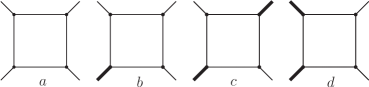
Figure 1: Diagrams corresponding to scattering of light by light, photon splitting and Delbrück scattering. The thick lines correspond to the off-shell photon.

To calculate the integral $I_{4}^{(d)}$, we will need integrals with fewer propagators:

$$I_{3}^{(d)}(m_{1}^{2},m_{2}^{2},m_{3}^{2};s_{23},s_{13},s_{12})=\frac{1}{i\pi^{d/2}}\int\frac{d^{d}k_{1}}{D_{1}D_{2}D_{3}},$$ (2.3)

$$I_{2}^{(d)}(m_{1}^{2},m_{2}^{2};s_{12})=\frac{1}{i\pi^{d/2}}\int\frac{d^{d}k_{1}}{D_{1}D_{2}},$$ (2.4)

$$I_{1}^{(d)}(m_{1}^{2})=\frac{1}{i\pi^{d/2}}\int\frac{d^{d}k_{1}}{D_{1}}.$$ (2.5)

The formula for functional reduction of the integral $I_{4}^{(d)}$ with arbitrary masses and kinematic variables Tarasov:2022clb can be represented as,

$$I_{4}^{(d)}(m_{1}^{2},m_{2}^{2},m_{3}^{2},m_{4}^{2};s_{12},s_{23},s_{34},s_{14},s_{24},s_{13})$$

$$~{}~{}~{}~{}~{}~{}~{}~{}~{}~{}~{}~{}~{}~{}~{}~{}~{}~{}~{}~{}~{}~{}~{}~{}~{}~{}~{}~{}=\sum_{k=1}^{24}Q_{k}{B_{4}^{(d)}(}R^{(k)}_{1},R^{(k)}_{2},R^{(k)}_{3},R^{(k)}_{4}),$$ (2.6)

where $R^{(k)}_{j}$ are the ratios of the modified Cayley determinant to the Gram determinant, $Q_{k}$ are products of the ratios of polynomials in the squared masses and kinematic variables $s_{ij}$. The function $B_{4}^{(d)}$ is defined as follows

$${B_{4}^{(d)}(R_{1},R_{2},R_{3},R_{4})}$$

$$~{}~{}~{}=I_{4}^{(d)}(R_{1},R_{2},R_{3},R_{4};R_{2}\!-\!R_{1},R_{3}\!-\!R_{2},R_{4}\!-\!R_{3},R_{4}\!-\!R_{1},R_{4}\!-\!R_{2},R_{3}\!-\!R_{1})$$

$$~{}~{}~{}=\Gamma\left(4-\frac{d}{2}\right)R_{1}^{\frac{d}{2}-4}\int_{0}^{1}\int_{0}^{1}\int_{0}^{1}x_{1}^{2}x_{2}~{}h_{4}^{\frac{d}{2}-4}dx_{1}dx_{2}dx_{3},$$ (2.7)

$$h_{4}=1-z_{1}x_{1}^{2}-z_{2}x_{1}^{2}x_{2}^{2}-z_{3}x_{1}^{2}x_{2}^{2}x_{3}^{2}.$$

The variables $z_{j}$ are simple combinations of $R_{i}$

$$z_{1}=1-\frac{R_{2}}{R_{1}},~{}~{}~{}~{}z_{2}=\frac{R_{2}-R_{3}}{R_{1}},~{}~{}~{}~{}z_{3}=\frac{R_{3}-R_{4}}{R_{1}}.$$ (2.8)

An explicit formula for the functional reduction of the integral $I_{4}^{(d)}$ is presented in Tarasov:2022clb .

3 Integral $I_{4}^{(d)}$ for the light by light scattering amplitude

The integral required for computing the light by light scattering amplitude corresponds to the following values of kinematic variables and masses

$$s_{12}=s_{23}=s_{34}=s_{14}=0,~{}~{}~{}~{}~{}~{}m_{j}^{2}=m^{2},~{}~{}~{}~{}j=1,...,4.$$ (3.9)

Inserting these values in the final formula for functional reduction of the integral $I_{4}^{(d)}$, given in Tarasov:2022clb , we get

$$I_{4}^{(d)}(m^{2},m^{2},m^{2},m^{2};0,0,0,0,s_{24},s_{13})=$$

$$~{}~{}~{}~{}~{}~{}~{}~{}~{}~{}~{}~{}~{}~{}~{}\frac{\tilde{s}_{13}}{(\tilde{s}_{24}+\tilde{s}_{13})}L^{(d)}(\tilde{s}_{13},M_{2}^{2},m^{2})+\frac{\tilde{s}_{24}}{(\tilde{s}_{24}+\tilde{s}_{13})}L^{(d)}(\tilde{s}_{24},M_{2}^{2},m^{2}),$$ (3.10)

where

$$L^{(d)}(\tilde{s}_{ij},M_{2}^{2},m^{2})=$$

$$~{}~{}~{}~{}~{}~{}I_{4}^{(d)}\left(m^{2}-M_{2}^{2},m^{2},m^{2}-\tilde{s}_{ij},m^{2};M^{2}_{2},-\tilde{s}_{ij},\tilde{s}_{ij},M^{2}_{2},0,M^{2}_{2}-\tilde{s}_{ij}\right),~{}~{}~{}~{}~{}$$ (3.11)

$$M^{2}_{2}=\frac{\tilde{s}_{24}\tilde{s}_{13}}{(\tilde{s}_{24}+\tilde{s}_{13})},~{}~{}~{}~{}~{}~{}~{}\tilde{s}_{ij}=\frac{s_{ij}}{4}.$$ (3.12)

The resulting formula (3.10) represents the integral $I_{4}^{(d)}$ depending on three variables in terms of integrals also depending on three variables. However, calculating the integral $L^{(d)}$ is simpler than calculating the original integral. We will consider different methods of calculating $L^{(d)}$.

It turns out that the recurrence equation with respect to $d$ provides an easy way to derive a compact expression for the function $L^{(d)}$. Such an equation for the integral $L^{(d)}(\tilde{s}_{ij},M_{2}^{2},m^{2})$ has the form Tarasov:2022clb :

$$(d-3)L^{(d+2)}(\tilde{s}_{ij},M_{2}^{2},m^{2})=-2m^{2}_{0}L^{(d)}(\tilde{s}_{ij},M_{2}^{2},m^{2})-I_{3}^{(d)}(m^{2};\tilde{s}_{ij}),$$ (3.13)

where

$$I_{3}^{(d)}(m^{2};\tilde{s}_{ij})=I_{3}^{(d)}(m^{2},m^{2}-\tilde{s}_{ij},m^{2};\tilde{s}_{ij},0,-\tilde{s}_{ij}),$$ (3.14)

$$m_{0}^{2}=m^{2}-M_{2}^{2}.$$ (3.15)

The solution of the equation (3.13) can be represented as

$$L^{(d)}(\tilde{s}_{ij},M^{2}_{2},m^{2})$$

$$~{}~{}~{}~{}~{}~{}~{}=\frac{(m_{0}^{2})^{\frac{d}{2}}~{}c_{4}^{(d)}(\tilde{s}_{ij},M^{2}_{2},m^{2})}{\Gamma\left(\frac{d-3}{2}\right)\sin\frac{\pi d}{2}}-\frac{1}{2m_{0}^{2}}\sum_{r=0}^{\infty}\frac{\left(\frac{d-3}{2}\right)_{r}}{(-m_{0}^{2})^{r}}I_{3}^{(d+2r)}(m^{2};\tilde{s}_{ij}),$$ (3.16)

where $c_{4}^{(d+2)}(\tilde{s}_{ij},M^{2}_{2},m^{2})=c_{4}^{(d)}(\tilde{s}_{ij},M^{2}_{2},m^{2})$ is an arbitrary periodic function of the parameter $d$. Using the method of ref. Tarasov:2015wcd , we obtained for the integral $I_{3}^{(d)}(m^{2};\tilde{s}_{ij})$ a simple functional relation

$$I_{3}^{(d)}(m^{2};\tilde{s}_{ij})=I_{3}^{(d)}(m^{2},m^{2},m^{2};4\tilde{s}_{ij},0,0),$$ (3.17)

which reduces this integral to the well-known result Boos:1990rg

$$I_{3}^{(d)}(m^{2};\tilde{s}_{ij})=-\frac{(m^{2})^{\frac{d}{2}-3}}{2}\Gamma\left(3-\frac{d}{2}\right)\,{}_{3}F_{2}\!\!\left[\begin{array}[]{c}1,1,3-\frac{d}{2}\,;\\ 2,\frac{3}{2}\,;\end{array}\frac{s_{ij}}{4m^{2}}\right].$$ (3.20)

We find the function $c_{4}^{(d)}(\tilde{s}_{ij},M^{2}_{2},m^{2})$ as a solution of a differential equation that can be obtained, for example, from a differential equation for the integral $L^{(d)}(\tilde{s}_{ij},M_{2}^{2},m^{2})$

$$\tilde{s}_{ij}\frac{\partial}{\partial\tilde{s}_{ij}}L^{(d)}(\tilde{s}_{ij},M_{2}^{2},m^{2})=-L^{(d)}(\tilde{s}_{ij},M_{2}^{2},m^{2})$$

$$~{}~{}~{}~{}~{}~{}~{}~{}~{}~{}~{}~{}~{}~{}~{}+\frac{(d-3)}{8(M_{2}^{2}-\tilde{s}_{ij})(M_{2}^{2}-m^{2})}I^{(d)}_{2}(m^{2}-M_{2}^{2},m^{2};M_{2}^{2})$$

$$~{}~{}~{}~{}~{}~{}~{}~{}~{}~{}~{}~{}~{}~{}~{}-\frac{(d-3)}{8(M_{2}^{2}-\tilde{s}_{ij})(\tilde{s}_{ij}-m^{2})}I_{2}^{(d)}(m^{2}-\tilde{s}_{ij},m^{2};\tilde{s}_{ij})$$

$$~{}~{}~{}~{}~{}~{}~{}~{}~{}~{}~{}~{}~{}~{}~{}+\frac{(d-2)}{16m^{2}(\tilde{s}_{ij}-m^{2})(M_{2}^{2}-m^{2})}I_{1}^{(d)}(m^{2}).$$ (3.21)

This equation was obtained under the assumption that $\tilde{s}_{ij}$ and $M_{2}^{2}$ are independent variables. Substituting the solution (3.16) into the equation (3.21), we get a simple differential equation

$$\tilde{s}_{ij}\frac{\partial c_{4}^{(d)}(\tilde{s}_{ij},M_{2}^{2},m^{2})}{\partial\tilde{s}_{ij}}+c_{4}^{(d)}(\tilde{s}_{ij},M_{2}^{2},m^{2})=0.$$ (3.22)

The solution of this equation is

$$c_{4}^{(d)}(\tilde{s}_{ij},M_{2}^{2},m^{2})=\frac{\tilde{c}_{4}^{(d)}(M_{2}^{2},m^{2})}{\tilde{s}_{ij}},$$ (3.23)

where $\tilde{c}_{4}^{(d)}(M_{2}^{2},m^{2})$ is the integration constant of the differential equation (3.22). Using the boundary value of the integral $L^{(d)}$ at $\tilde{s}_{ij}=0$, we get

$$c_{4}^{(d)}(\tilde{s}_{ij},M_{2}^{2},m^{2})=0.$$ (3.24)

For the hypergeometric function from the equation (3.20), we used the following representation rainville1960special

$$\,{}_{3}F_{2}\!\!\left[\begin{array}[]{c}1,1,3-\frac{d}{2}\,;\\ 2,\frac{3}{2}\,;\end{array}x\right]=\frac{-\Gamma\left(\frac{3}{2}\right)}{x\Gamma\left(3-\frac{d}{2}\right)\Gamma\left(\frac{d-3}{2}\right)}\int_{0}^{1}dzz^{\frac{2-d}{2}}(1-z)^{\frac{d-5}{2}}\ln(1-xz).~{}~{}~{}~{}$$ (3.27)

Employing this representation and taking into account equation (3.24), the solution (3.16) can be written as

$$L^{(d)}(\tilde{s}_{ij},M_{2}^{2},m^{2})=-\frac{\pi^{\frac{1}{2}}(m^{2})^{\frac{d}{2}-3}}{8\tilde{s}_{ij}\Gamma\left(\frac{d-3}{2}\right)}\int_{0}^{1}\frac{dz~{}z^{2-\frac{d}{2}}(1-z)^{\frac{d-5}{2}}}{1-z\frac{M_{2}^{2}}{m^{2}}}\ln\left(1-z\frac{\tilde{s}_{ij}}{m^{2}}\right).$$ (3.28)

Substituting this expression into the equation (3.10), we get

$$I_{4}^{(d)}(m^{2},m^{2},m^{2},m^{2};0,0,0,0,s_{24},s_{13})=-\frac{\pi^{\frac{1}{2}}(m^{2})^{\frac{d}{2}-3}}{2(s_{24}+s_{13})\Gamma\left(\frac{d-3}{2}\right)}~{}~{}~{}~{}~{}~{}~{}~{}~{}~{}~{}$$

$$~{}~{}~{}~{}~{}~{}~{}~{}~{}~{}\times\int_{0}^{1}\frac{dz~{}z^{2-\frac{d}{2}}(1-z)^{\frac{d-5}{2}}}{1-z\frac{M_{2}^{2}}{m^{2}}}\left[\ln\left(1-z\frac{s_{13}}{4m^{2}}\right)+\ln\left(1-z\frac{s_{24}}{4m^{2}}\right)\right].~{}~{}~{}$$ (3.29)

This is the simplest representation known so far for this integral. Note that for $d=4$ in ref. Davydychev:1993ut , this integral was obtained in terms of the hypergeometric Appell function $F_{3}$, which was expressed as a two-fold integral.

The representation (3.28) is convenient for a series expansion in $\varepsilon=(4-d)/2$. For $d=4$, we have

$$L^{(4)}(\tilde{s}_{ij},M_{2}^{2},m^{2})=\frac{-1}{8M_{2}^{2}{s}_{ij}\beta_{2}}\left[\ln^{2}\frac{\beta_{ij}+1}{\beta_{2}-\beta_{ij}}-\frac{1}{2}\ln^{2}\frac{\beta_{2}-\beta_{ij}}{\beta_{2}+\beta_{ij}}-\ln\frac{\beta_{ij}-1}{\beta_{ij}+1}\ln\frac{\beta_{2}-\beta_{ij}}{\beta_{2}+\beta_{ij}}\right.$$

$$\left.+\frac{\pi^{2}}{3}+2{\mbox{Li}}_{2}\left(\frac{\beta_{ij}-\beta_{2}}{\beta_{ij}+1}\right)-2{\mbox{Li}}_{2}\left(\frac{\beta_{ij}-1}{\beta_{2}+\beta_{ij}}\right)+{\mbox{Li}}_{2}\left(\frac{\beta_{ij}^{2}-1}{\beta_{ij}^{2}-\beta_{2}^{2}}\right)\right].~{}~{}~{}~{}~{}~{}~{}~{}$$ (3.30)

where

$$\beta_{ij}\equiv\sqrt{1-\frac{m^{2}}{\tilde{s}_{ij}}},~{}~{}~{}~{}(ij=13,24)\;\;~{}~{}~{}~{}~{}~{}~{}~{}~{}~{}~{}\beta_{2}\equiv\sqrt{1-\frac{m^{2}}{M_{2}^{2}}}.\;$$ (3.31)

Using (3.30), from the equation (3.10), we get

$$I_{4}^{(4)}(m^{2},m^{2},m^{2},m^{2};0,0,0,0,s_{24},s_{13})$$

$$=\frac{1}{8\tilde{s}_{13}\tilde{s}_{24}\beta_{2}}\left\{2\ln^{2}\left(\frac{\beta_{2}+\beta_{13}}{\beta_{2}+\beta_{24}}\right)+\ln\left(\frac{\beta_{2}-\beta_{13}}{\beta_{2}+\beta_{13}}\right)\;\ln\left(\frac{\beta_{2}-\beta_{24}}{\beta_{2}+\beta_{24}}\right)-\frac{\pi^{2}}{2}\right.\hskip 28.45274pt$$

$$\left.+\sum_{i=13,24}\left[2{\mbox{Li}}_{2}\left(\frac{\beta_{i}-1}{\beta_{2}+\beta_{i}}\right)-2{\mbox{Li}}_{2}\left(-\frac{\beta_{2}-\beta_{i}}{\beta_{i}+1}\right)-\ln^{2}\left(\frac{\beta_{i}+1}{\beta_{2}+\beta_{i}}\right)\right]\right\}.~{}~{}~{}~{}~{}~{}~{}~{}~{}$$ (3.32)

In the sum of two $L^{(d)}$ the third terms with $\rm Li_{2}$ from (3.30) cancel. The expression (3.32) agrees with the result obtained in ref. Davydychev:1993ut .

The function $L^{(d)}$ can be obtained as a solution to the equation (3.21). For $d=4$, the solution of this equation has the form

$$L^{(4)}(\tilde{s}_{ij},M_{2}^{2},m^{2})=\frac{1}{8s_{ij}M_{2}^{2}\beta_{2}}\Biggl{[}F(y_{ij},y_{2})-2{\rm Li_{2}}\left(1-y_{2}\right)\Biggr{]},~{}~{}~{}~{}~{}~{}$$ (3.33)

where

$$F(y_{ij},y_{k})={\rm Li}_{2}\left(1-y_{ij}y_{k}\right)+{\rm Li}_{2}\left(1-\frac{y_{k}}{y_{ij}}\right)+\frac{1}{2}\ln^{2}y_{ij},$$ (3.34)

$$y_{ij}=\frac{\beta_{ij}-1}{\beta_{ij}+1},~{}~{}~{}~{}~{}~{}y_{2}=\frac{\beta_{2}-1}{\beta_{2}+1}.$$ (3.35)

Note that the expression (3.33) is invariant as with respect to the replacement of $y_{ij}\rightarrow 1/y_{ij}$ and with respect to the replacement $y_{2}\rightarrow 1/y_{2}$.

Substituting (3.33) into the formula (3.10), we get

$$I_{4}^{(d)}(m^{2},m^{2},m^{2},m^{2};0,0,0,0,s_{24},s_{13})$$

$$~{}~{}~{}~{}~{}=\frac{1}{2s_{13}s_{24}\beta_{2}}\Biggl{[}F(y_{13},y_{2})+F(y_{24},y_{2})-4{\rm Li_{2}}\left(1-y_{2}\right)\Biggr{]}.~{}~{}~{}$$ (3.36)

Series representations of $L^{(d)}(\tilde{s}_{ij},M_{2}^{2},m^{2})$ can be obtained from the integral representations (2.7), (3.28).

4 Integral $I_{4}^{(d)}$ for the photon splitting amplitude

In this section, we turn to the integral with one external line off-shell, which is associated with the diagram $b)$ in Figure 1. This integral corresponds to the kinematics

$$s_{23}=s_{34}=s_{14}=0,~{}~{}~{}~{}~{}~{}m_{i}^{2}=m^{2}.$$ (4.37)

Using the final formula for functional reduction of $I_{4}^{(d)}$ from ref. Tarasov:2022clb , we get

$$(s_{12}-s_{24}-s_{13})I_{4}^{(d)}(m^{2},m^{2},m^{2},m^{2},s_{12},0,0,0,s_{24},s_{13})$$

$$~{}~{}~{}~{}=s_{12}L^{(d)}(\tilde{s}_{12},M_{3}^{2},m^{2})-s_{13}L^{(d)}(\tilde{s}_{13},M_{3}^{2},m^{2})-s_{24}L^{(d)}(\tilde{s}_{24},M_{3}^{2},m^{2}).~{}~{}~{}~{}$$ (4.38)

where

$$M_{3}^{2}=\frac{s_{24}s_{13}}{4(s_{13}+s_{24}-s_{12})}.$$ (4.39)

For $d=4$, we have

$$I_{4}^{(4)}(m^{2},m^{2},m^{2},m^{2},s_{12},0,0,0,s_{24},s_{13})$$

$$~{}~{}~{}~{}~{}~{}~{}~{}=\frac{F(y_{13},y_{3})+F(y_{24},y_{3})-F(y_{12},y_{3})-2{\rm Li}_{2}(1-y_{3})}{2{s}_{24}{s}_{13}\beta_{3}},$$ (4.40)

where

$$y_{3}=\frac{\beta_{3}-1}{\beta_{3}+1},~{}~{}~{}~{}~{}\beta_{3}=\sqrt{1-\frac{m^{2}}{M_{3}^{2}}}.$$ (4.41)

5 Integrals $I_{4}^{(d)}$ for the Delbrück scattering amplitude

We now turn to the more complicated integrals corresponding to the diagrams $c)$ and $d)$ in Figure 1.

Inserting the values of masses and kinematic variables for the integral represented by the diagram $c)$,

$$s_{23}=s_{14}=0,~{}~{}~{}~{}~{}m_{k}^{2}=m^{2},~{}~{}~{}k=1,...,4,$$ (5.42)

in the final formula for the functional reduction of $I_{4}^{(d)}$ from ref. Tarasov:2022clb , we get

$$(s_{12}-s_{13}-s_{24}+s_{34})I_{4}^{(d)}(m^{2},m^{2},m^{2},m^{2};s_{12},0,s_{34},0,s_{24},s_{13})$$

$$~{}~{}~{}~{}~{}~{}~{}~{}~{}~{}~{}~{}~{}~{}~{}~{}=s_{12}L^{(d)}(\tilde{s}_{12},M_{4}^{2},m^{2})-s_{13}L^{(d)}(\tilde{s}_{13},M_{4}^{2},m^{2})$$

$$~{}~{}~{}~{}~{}~{}~{}~{}~{}~{}~{}~{}~{}~{}~{}~{}-s_{24}L^{(d)}(\tilde{s}_{24},M_{4}^{2},m^{2})+s_{34}L^{(d)}(\tilde{s}_{34},M_{4}^{2},m^{2}),~{}~{}~{}~{}~{}$$ (5.43)

where

$$M^{2}_{4}=\frac{s_{12}s_{34}-s_{13}s_{24}}{4(s_{12}-s_{13}-s_{24}+s_{34})}.$$ (5.44)

At $d=4$, we obtain

$$I_{4}^{(4)}(m^{2},m^{2},m^{2},m^{2};s_{12},0,s_{34},0,s_{24},s_{13})$$

$$~{}~{}~{}~{}~{}~{}~{}~{}~{}~{}~{}=\frac{F(y_{13},y_{4})+F(y_{24},y_{4})-F(y_{34},y_{4})-F(y_{12},y_{4})}{2({s}_{13}{s}_{24}-{s}_{12}{s}_{34})\beta_{4}},~{}~{}~{}$$ (5.45)

where

$$y_{4}=\frac{\beta_{4}-1}{\beta_{4}+1},~{}~{}~{}~{}~{}\beta_{4}=\sqrt{1-\frac{m^{2}}{M_{4}^{2}}}.$$ (5.46)

Another integral contributing to Delbrück scattering cross section is represented by the diagram $d)$ in Figure 1. The kinematics corresponding to this diagram reads

$$s_{34}=s_{14}=0,~{}~{}~{}~{}m_{k}^{2}=m^{2},~{}~{}~{}~{}k=1,...4.$$ (5.47)

Substituting these values into the final formula for functional reduction Tarasov:2022clb , we obtain

$$d_{1}d_{2}I_{4}^{(d)}(m^{2},m^{2},m^{2},m^{2};s_{12},s_{23},0,0,s_{24},s_{13})$$

$$=\frac{1}{2}d_{1}s_{13}s_{24}I_{4}^{(d)}(m_{0}^{2},m^{2},m^{2}-\tilde{s}_{13},m^{2})-\frac{1}{2}d_{1}s_{23}s_{24}I_{4}^{(d)}(m_{0}^{2},m^{2},m^{2}-\tilde{s}_{23},m^{2})$$

$$-~{}\frac{1}{2}d_{1}s_{12}s_{24}I_{4}^{(d)}(m_{0}^{2},m^{2},m^{2}-\tilde{s}_{12},m^{2})+d_{1}s_{24}^{2}I_{4}^{(d)}(m_{0}^{2},m^{2},m^{2}-\tilde{s}_{24},m^{2})$$

$$+~{}\frac{1}{2}n_{1}s_{12}(s_{12}-s_{13}-s_{23})I_{4}^{(d)}(m_{0}^{2},\tilde{m}^{2}_{0},m^{2}-\tilde{s}_{12},m^{2})$$

$$-~{}\frac{1}{2}n_{1}s_{13}(s_{12}-s_{13}+s_{23})I_{4}^{(d)}(m_{0}^{2},\tilde{m}^{2}_{0},m^{2}-\tilde{s}_{13},m^{2})$$

$$-~{}\frac{1}{2}n_{1}s_{23}(s_{12}+s_{13}-s_{23})I_{4}^{(d)}(m_{0}^{2},\tilde{m}^{2}_{0},m^{2}-\tilde{s}_{23},m^{2}),$$ (5.48)

where

$$m_{0}^{2}=m^{2}-\tilde{s}_{1},~{}~{}~{}~{}~{}~{}\tilde{m}^{2}_{0}=m^{2}-\tilde{s}_{2},~{}~{}~{}~{}~{}~{}\tilde{s}_{1}=\frac{s_{13}s_{24}^{2}}{4d_{2}},~{}~{}~{}~{}~{}~{}\tilde{s}_{2}=-\frac{s_{12}s_{13}s_{23}}{d_{1}},$$ (5.49)

$$n_{1}=2s_{12}s_{23}-s_{12}s_{24}+s_{13}s_{24}-s_{23}s_{24},$$

$$d_{1}=s_{12}^{2}+s_{13}^{2}+s_{23}^{2}-2s_{12}s_{13}-2s_{12}s_{23}-2s_{13}s_{23},$$

$$d_{2}=s_{12}s_{23}-s_{12}s_{24}+s_{13}s_{24}-s_{23}s_{24}+s_{24}^{2}.$$ (5.50)

The first four integrals in the equation (5.48) are expressed in terms of the function $L^{(d)}$. The three remaining integrals $I_{4}^{(d)}(m_{0}^{2},\tilde{m}^{2}_{0},m^{2}-\tilde{s}_{ij},m^{2})$, can be calculated using the formula from ref. Tarasov:2022clb

$$I_{4}^{(d)}(r_{1234},r_{234},r_{34},r_{4})=\int_{0}^{1}\int_{0}^{1}\!\int_{0}^{1}\frac{\Gamma\left(4-\frac{d}{2}\right)x_{1}^{2}x_{2}~{}dx_{1}dx_{2}dx_{3}}{\left[a-bx_{1}^{2}-cx_{1}^{2}x_{2}^{2}-ex_{1}^{2}x_{2}^{2}x_{3}^{2}\right]^{4-\frac{d}{2}}},~{}~{}~{}~{}~{}~{}~{}$$ (5.51)

where

$$a=r_{1234},~{}~{}~{}~{}~{}b=r_{1234}-r_{234},~{}~{}~{}~{}~{}c=r_{234}-r_{34},~{}~{}~{}~{}~{}e=r_{34}-r_{4}.$$ (5.52)

For $d=4$, the integral (5.51) can be calculated as a combination of functions $L^{(4)}$ with various arguments. The detailed derivation of the result will be described in an expanded version of this article.

6 Conclusions

Our results clearly indicate that the application of the functional reduction method makes it possible to reduce complicated integrals to simpler integrals. Even if the number of variables in the integrals resulting from applying the functional reduction is the same as in the original integral, these integrals are simpler than the original integral. In general, integrals depending on more than four variables are reduced to a combination of integrals with four or fewer variables, which are also simpler than the original integral.

The fact that the results for the integrals discussed in this paper are expressed in terms of the same function $L^{(d)}$ may be useful for improving the accuracy and efficiency of calculating radiative corrections. The integral representation (3.28) can significantly simplify the calculation of higher order terms in the $\varepsilon$ expansion of integrals considered in the article.

References

• (1) O. V. Tarasov. Functional reduction of one-loop Feynman integrals with arbitrary masses. JHEP, 06:155, 2 2022.
• (2) R. Karplus and M. Neuman. The scattering of light by light. Phys. Rev., 83:776–784, 1951.
• (3) R. Karplus and M. Neuman. Non-Linear Interactions between Electromagnetic Fields. Phys. Rev., 80:380–385, 1950.
• (4) B. De Tollis. Dispersive Approach to Photon-Photon Scattering. Nuovo Cim., 32:757, 1964.
• (5) B. De Tollis. The Scattering of Photons by Photons. Nuovo Cim., 35:1182, 1965.
• (6) V. Constantini, B. De Tollis, and G. Pistoni. Nonlinear Effect in Quantum Electrodynamics. Nuovo Cimento, 2A:733–787, 1971.
• (7) Y. Shima. Photon Splitting in a Nuclear Electric Field. Phys. Rev., 142(4):944, 1966.
• (8) V. N. Baier, Victor S. Fadin, V. M. Katkov, and E. A. Kuraev. Photon splitting into two photons in a coulomb field. Phys. Lett. B, 49:385–387, 1974.
• (9) G. Jikia and A. Tkabladze. Photon-photon scattering at the photon linear collider. Phys. Lett. B, 323:453–458, 1994.
• (10) G. J. Gounaris, P. I. Porfyriadis, and F. M. Renard. The gamma gamma —$>$ gamma gamma process in the standard and SUSY models at high-energies. Eur. Phys. J. C, 9:673–686, 1999.
• (11) M. Aaboud et al. Evidence for light-by-light scattering in heavy-ion collisions with the ATLAS detector at the LHC. Nature Phys., 13(9):852–858, 2017.
• (12) Albert M Sirunyan et al. Evidence for light-by-light scattering and searches for axion-like particles in ultraperipheral PbPb collisions at $\sqrt{s_{\mathrm{NN}}}=$ 5.02 TeV. Phys. Lett. B, 797:134826, 2019.
• (13) O. V. Tarasov. Derivation of Functional Equations for Feynman Integrals from Algebraic Relations. JHEP, 11:038, 2017.
• (14) E.E. Boos and A. I. Davydychev. A Method of evaluating massive Feynman integrals. Theor.Math.Phys., 89:1052–1063, 1991.
• (15) D. Rainville. Special functions. Macmillan, 1960.
• (16) A. I. Davydychev. Standard and hypergeometric representations for loop diagrams and the photon-photon scattering. In 7th International Seminar on High-energy Physics, 5 1993.