Synchronization transition of the second-order Kuramoto model on lattices

Abstract

The second-order Kuramoto equation describes synchronization of coupled oscillators with inertia, which occur in power grids for example. Contrary to the first-order Kuramoto equation it’s synchronization transition behavior is much less known. In case of Gaussian self-frequencies it is discontinuous, in contrast to the continuous transition for the first-order Kuramoto equation. Here we investigate this transition on large 2d and 3d lattices and provide numerical evidence of hybrid phase transitions, that the oscillator phases $\theta_{i}$, exhibit a crossover, while the frequency spread a real phase transition in 3d. Thus a lower critical dimension $d_{l}^{O}=2$ is expected for the frequencies and $d_{l}^{R}=4$ for the phases like in the massless case. We provide numerical estimates for the critical exponents, finding that the frequency spread decays as $\sim t^{-d/2}$ in case of aligned initial state of the phases in agreement with the linear approximation. However in 3d, in the case of initially random distribution of $\theta_{i}$, we find a faster decay, characterized by $\sim t^{-1.8(1)}$ as the consequence of enhanced nonlinearities which appear by the random phase fluctuations.

I Introduction

Synchronization within interacting systems is an ubiquitous phenomenon in nature. It has been observed in biological, chemical, physical, and sociological systems. Much effort has been dedicated for theoretical understanding of its general features Pikovsky et al. (2003); Acebrón et al. (2005); Arenas et al. (2008). A paradigmatic model of $N$ globally coupled oscillators was introduced and solved in the stationary state in the limit $N\to\infty$ by Kuramoto Kuramoto (1975) and later the macroscopic evolution of the system was shown to be governed by a finite set of nonlinear ordinary differential equations Ott and Antonsen (2008). An interesting property of the so-called first-order Kuramoto model is that it has a continuous phase transition, with a diverging correlation size, separating a synchronized phase from an unsynchronized one. Due to the chaoticity, emerging from nonlinearity, it obeys a scaling theory, analogous to stochastic systems at the critical point and the whole set of critical exponents are known Kuramoto (1975); Ott and Antonsen (2008); Hong et al. (2007); Choi et al. (2013). The corresponding universality class is termed as mean-field since, due to the all-to-all coupling, the individual oscillators interact with a mean-field of the rest of the oscillators. A challenging research direction aims at studying the possibility and nature of synchronization transitions in extended systems, where oscillators are fixed at regular lattice sites of finite dimension $d$ and the interaction, in the extreme case, is restricted to nearest-neighbors Sakaguchi et al. (1987); Hong et al. (2005, 2007); Juhász et al. (2019).

The so-called second-order Kuramoto model was proposed to describe power grids, analogous to the swing equation of AC circuits Filatrella et al. (2008). This is the generalization of the Kuramoto model Kuramoto (1975) with inertia. One of the main consequences of this inertia is that the second-order phase synchronization transition, observed in the mean-field models of the massless first-order Kuramoto models turns into a first-order one Tanaka et al. (1997).

However, in lower dimensions this has not been studied systematically. In Ódor and Hartmann (2018) numerical integration on 2d lattices suggested crossover transitions, with hysteresis in case of the phase order parameter. Note, that due to the inherent heterogeneity of the quenched self-frequencies $\omega_{i}(0)$ of the nodes, rare-region effects may occur, leading to frustrated synchronization and chimera states Ódor and Hartmann (2018); Villegas et al. (2014); Millán et al. (2018); Ódor et al. (2022).

As real power grids are connected via complex networks, topological heterogeneity are also present, which can smear a phase transition, strengthening possible rare-region effects. However, even if topological heterogeneity are not present, it is still not proven yet whether the massive model exhibit real phase transitions at low dimensions. Only conjectures, that the massive model has the same lower and upper critical dimensions as the first-order Kuramoto model , are available. Accordingly, mean-field phase transition for $d\geq 4$ of the phase order parameter and a crossover below it Acebrón et al. (2005) should occur . Thus, the upper and lower critical dimensions may be identical: $d_{c}=d_{l}=4$.

For the frequency entrainment of the massless model the lower critical dimension is expected to be at $d_{l}^{O}=2$ similar to the Mermin-Wagner theorem Mermin and Wagner (1966) for the planar XY spin model and is supported by finite size scaling analysis Hong et al. (2005). Thus, for intermediate dimensions $2<d<4$, real, nontrivial continuous phase transition should occur. Analogously, for the massive case Ódor and Hartmann (2018, 2020); Ódor et al. (2022), entrainment phase transition is also expected for dimensions $2<d<4$, as a very recent power-grid study Ódor et al. (2022) has indicated it for networks with graphs dimensions $2<d<3$.

This has recently been published for the high voltage power-grid networks of the USA and Europe and now we shall investigate it in case of pure 2d and 3d lattices, using finite size scaling. In that work the linear approximation, which is expected to be valid for large couplings, provided a frequency spread decay law $\Omega\sim t^{-d/2}$ Ódor et al. (2022). Now we test the applicability of this approximation at the phase transition points.

Besides the dynamical scaling the frequency order parameter exhibited a hysteresis and a discontinuity Ódor et al. (2022), which is known in statistical physics Cardy (1981), termed as hybrid or mixed type of phase transition, for example at tricriticality Janssen et al. (2004); Chan et al. (2015), or in other nonequilibrium systems Gómez-Gardeñes et al. (2011); Coutinho et al. (2013); Ódor and de Simoni (2021). Now we investigate in detail this transition, which arises by the inertia in the Kuramoto model and results in hysteresis as we change the synchronization level of the initial states.

II Models and methods

II.1 The second-order Kuramoto model

Time evolution of power grids synchronization is described by the swing equations Grainger and Stevenson (1994), set up for mechanical elements with inertia. It is formally equivalent to the second-order Kuramoto equation Filatrella et al. (2008), for a network of $N$ oscillators with phases $\theta_{i}(t)$:

$$\dot{\theta_{i}}(t) = \omega_{i}(t)$$ (1)

$$\dot{\omega_{i}}(t) = \omega_{i}(0)-\alpha\dot{\theta_{i}}(t)+K\sum_{j=1}^{N}A_{ij}\sin[\theta_{j}(t)-\theta_{i}(t)]\ .$$

Here $\alpha$ is the damping parameter, which describes the power dissipation, or an instantaneous feedback Ódor and Hartmann (2020), $K$ is the global coupling, related to the maximum transmitted power between nodes and $A_{ij}$, which is the adjacency matrix of the network, containing admittance elements. The quenched self-frequency of the $i$-th oscillator is $\omega_{i}(0)$, which describes the power in/out of a given node when Eq. (1) is considered to be the swing equation of a coupled AC circuit, but here we have chosen it zero centered Gaussian random variable as rescaling invariance of the equation allows to transform it within a rotating frame.

In our present study the following parameter settings were used: the dissipation factor $\alpha$, is chosen to be equal to $0.4$ to meet expectations for power-grids, with the $[1/s]$ inverse time physical dimension assumption. For modeling instantaneous feedback, or increased damping parameter we also investigated the $\alpha=3.0\,[1/s]$ case, similarly as in Ódor and Hartmann (2020); Ódor et al. (2022).

To solve the differential equations in general we used the adaptive Bulirsch‐Stoer stepper Ahnert and Mulansky , which provides more precise results for large $K$ coupling values than the Runge-Kutta method. The solutions depend on the $\omega_{i}(0)$ values and become chaotic, especially at the synchronization transition, and thus to obtain reasonable statistics, we needed strong computing resources, using parallel codes running on GPU clusters. The corresponding CUDA code allowed us to achieve $\sim 100\times$ speedup on GeForce GTX 1080 cards as compared to Intel(R) Core(TM) i7-4930K CPU @ 3.40GHz cores. The details of the GPU implementation will be discussed in a separate publication Jeffrey et al. (to be published).

We obtain larger synchronization if the initial state is set to be fully synchronized, with phases: $\theta_{i}(0)=0$, but due to the hysteresis one can also investigate other uniform random distributions like: $\theta_{i}(0)\in(0,2\pi)$. The initial frequencies were set as: $\dot{\theta_{i}}(0)=\omega_{i}(0)$.

To characterize the phase transition properties, both the phase order parameter $R(t)$ and the frequency spread $\Omega(t)$, termed the frequency order parameter, will be studied. We measured the Kuramoto phase order parameter:

$$z(t_{k})=r(t_{k})\exp{i\theta(t_{k})}=1/N\sum_{j}\exp{[i\theta_{j}(t_{k})}]\ ,$$ (2)

by increasing the sampling time steps exponentially:

$$t_{k}=1+1.08^{k}\ ,$$ (3)

where $0\leq r(t_{k})\leq 1$ gauges the overall coherence and $\theta(t_{k})$ is the average phase. The set of equations (1) were solved numerically for $10^{3}-10^{4}$ independent initial conditions, initialized by different $\omega_{i}(0)$-s and different $\theta_{i}(0)$-s if a disordered initial phases were invoked. Then sample averages for the phases

$$R(t_{k})=\langle r(t_{k})\rangle$$ (4)

and for the variance of the frequencies

$$\Omega(t_{k},N)=\frac{1}{N}\sum_{j=1}^{N}(\overline{\omega}-\omega_{j})^{2}$$ (5)

were determined, where $\overline{\omega}(t_{k})$ denotes the mean frequency within each respective sample.

In the steady state, which we determined by visual inspection of the mean values $R(t_{k})$, we measured the standard deviations $\sigma(R)$ of the order parameters $R(t_{k})$ in order to locate the transition point by fluctuation maxima. While the transition point for $\Omega(t_{k},N)$ is characterized by a sudden drop of the $\Omega(t\to\infty,N)$ or by an emergence of an algebraic decay of $\Omega(t)$ as we increase $K$. In case of the first-order Kuramoto equation the fluctuations of both order parameters show a maximum at the respective transition points Ódor et al. (2022). For the second-order Kuramoto, only the $\sigma(R(t_{k}))$ seems to have a peak at $K^{\prime}_{c}$, while for $\Omega(t_{k},N)$ we located a different transition point $K_{c}$, where the saturation to steady state value changed to a decay in the $t\to\infty$ limit.

II.2 Linear approximation for the the frequency entrainment

In Ref. Ódor et al. (2022), we showed that, similar to the first-order Kuramoto model, the frequency order parameter (5) decays as $\Omega\propto t^{-d/2}$ on a $d$-dimensional lattice in the large system size and large coupling constant limit Hong et al. (2005). By applying the linear approximation $\sin(x)\propto x$ and casting the continuum second-order Kuramoto equations into the momentum space, the phase velocity [$\omega(\mathbf{x},t)\equiv\dot{\theta}(\mathbf{x},t)$] is obtained Ódor et al. (2022)

$$\omega(\mathbf{k},t)= e^{-\frac{1}{2}t(\alpha+\Delta)}\Big{[}\omega(\mathbf{k},0)\big{(}(\Delta+2-\alpha)e^{\Delta t}$$

$$+\alpha+\Delta-2\big{)}-2Kk^{2}\theta(\mathbf{k},0)\left(e^{\Delta t}-1\right)\Big{]}/2\Delta\,,$$ (6)

where $\Delta=\sqrt{\alpha^{2}-4Kk^{2}}$. When initial disordered condition is considered, say $\theta(\mathbf{x},0)$ is uniformly distributed over $(0,\theta_{\mathrm{max}})$, one has $\langle\theta(\mathbf{x})\theta(\mathbf{x}^{\prime})\rangle=\theta_{\mathrm{max}}^{2}/4$, suggesting that $\langle\theta(\mathbf{k},0)\theta(\mathbf{k}^{\prime},0)\rangle=\mathbf{\delta}^{d}(\mathbf{k})\mathbf{\delta}^{d}(\mathbf{k}^{\prime})$. Hence, in the linear approximation, disorder from the initial condition doesn’t affect the frequency spread (note that $\langle\omega(\mathbf{k},0)\theta(\mathbf{k},0)\rangle=0$) and we have (the same as in Ref. Ódor et al. (2022)):

$$\Omega(t)= \frac{1}{L^{d}}\int d^{d}\mathbf{x}\langle\left[\omega(\mathbf{x},t)-\bar{\omega}(t)\right]^{2}\rangle$$

$$= C_{d}\int_{2\pi/L}^{\pi/a}dkk^{d-1}\frac{e^{-t(\alpha+\Delta)}}{4\Delta^{2}}\Big{[}\alpha+\Delta-2$$

$$+(\Delta-\alpha+2)e^{\Delta t}\Big{]}^{2}\,,$$ (7)

where $\bar{\omega}(t)$ denotes the spatial average of $\omega(\mathbf{x},t)$, while $a$ and $C_{d}$ are the lattice spacing and the geometric factor, respectively.

As shown in Ref. Ódor et al. (2022), Eq. (7) gives rise to the $t^{-d/2}$ law that manifests a rapid cutoff for large couplings in a typical finite system, whereas in the regime where a linear approximation is invalid, weak couplings fail to maintain a narrow frequency entrainment and $\Omega$ is bound to be stationary after some time. Hence, a frequency entrainment phase transition, from finite stationary $\Omega$ value to infinitely decaying $\Omega$ is expected.

III Synchronization transition in 2d

We solved the system of equations (1) on large square lattices with periodic boundary conditions for linear sizes: $L=200,\,400,\,1000,\,2000$. The self-frequencies were chosen randomly from a zero centered Gaussian distribution with unit variance. The order parameters were calculated by ensemble averages over many samples.

III.1 Frequency entrainment phase transition

It is known that the frequency order parameter (5) decays as $\Omega\propto t^{-d/2}$ in case of the first-order Kuramoto model in the large coupling limit if we start from a random initial state Hong et al. (2005). We have also shown that the same is true for the second-order Kuramoto model in the linear approximation in Ódor et al. (2022). Now we investigate this at the neighborhood of frequency entrainment transition point.

As Fig. 1 shows the density decays as $\Omega\propto t^{-1}$ at the critical coupling strength: $K_{c}=3.4(1)$ in the case of ordered phase initial conditions, for $\alpha=3$ damping factor. The decay behavior follows the same power law for $K\geq K_{c}$ before the finite size cutoff can take effect, and we see a saturation to finite values for $K<K_{c}$.

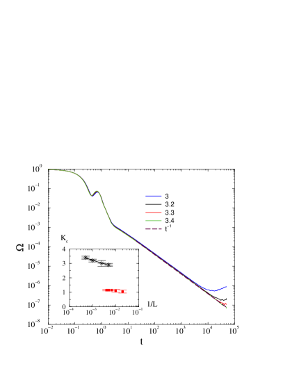
Figure 1: The frequency spread in 2d at $\alpha=3$ for different $K$ values, shown by the legends, for $L=2000$, in case of ordered initial conditions. The dashed line marks a numerical fit at the critical point $K_{c}=3.4(1)$ with $t^{-d/2}$. Inset: finite size scaling of the frequency entrainment transition point $K_{c}$ for various system sizes in 2d (black asterisks) and 3d (red boxes), for $\alpha=3$ and ordered initial conditions. One can see a logarithmic growth in 2d and a convergence to $K_{c}=1.15(5)$ constant value in 3d.

The same is true for $\alpha=0.4$: following a longer initial transient we can see a decay at $K_{c}=3.5(5)$ characterized by $\Omega\propto t^{-1}$. as shown by Fig. 2. An exponential finite size cutoff occurs already for $t>1000$ in contrast to the $\alpha=3$ case, where this happened above $t>10^{4}$.

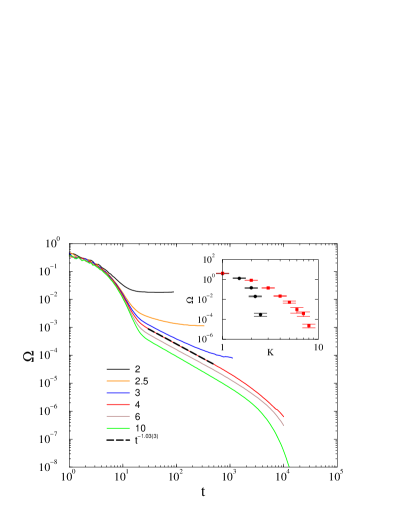
Figure 2: The frequency spread in 2d at $\alpha=0.4$ for different $K$ values, shown by the legends, for $L=2000$, using ordered initial conditions. The dashed line marks a numerical fit at the critical point $K_{c}=3.5(5)$ with $t^{-1.03(3)}$. Inset: Steady state values obtained by starting from ordered (black bullets) and disordered (red boxes) initial conditions.

For smaller system sizes the $K_{c}$-s do not move a lot, as we can see from the inset of Fig. 1. The available data precision restricts finite size scaling, but still we attempted it as shown in the inset of Fig. 1. Assuming a logarithmic growth dependence, which is expected at the lower critical dimension Hong et al. (2005) we obtained $K_{c}(1/L)\propto-1.7(1)\ln(1/L)$.

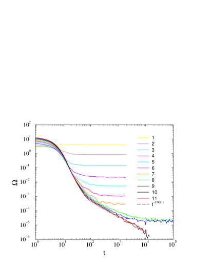
Figure 9: The frequency spread in 2d at $\alpha=0.4$ for different $K$ values, shown by the legends for $L=2000$, with disordered initial conditions. The dashed line marks a numerical fit at the critical point at $K_{c}=9.5(5)$ with $t^{-0.96(5)}$.

In the case of fully disordered initial conditions, $\theta_{i}(t=0)\in(0,2\pi)$, we found the same behavior as in case of the fully phase synchronized starts, as one can see on Fig. 3 for $\alpha=3$ and Fig. 9 for $\alpha=0.4$ shown in the Appendix.

The steady state values, appearing for $t>10^{4}$ near the critical point of the $\alpha=0.4$ damping factor case are also determined and plotted in the inset of Fig. 2 for $L=200$. We can see two branches, depending on the initial conditions. The upper branch corresponds to the disordered, the lower to the fully ordered initial states. Thus we can see a hysteresis like behavior near the phase transition. But the approach of $\Omega(K\to K_{c})$ is rather smooth, which is not surprising at a crossover point.

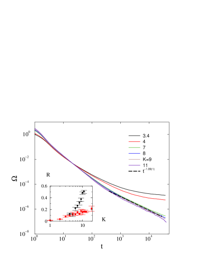
Figure 3: The frequency spread in 2d at $\alpha=3$ for different $K$ values, shown by the legends, for $L=2000$, in case of disordered initial conditions. The dashed line marks a numerical fit at the critical point at $K_{c}=8.0(5)$ with $t^{-1.09(5)}$. Inset: Part of the hysteresis loop of $R$ in 2d obtained by ordered (black bullets) and disordered (red boxes) initial conditions for $\alpha=3$ and $L=200$.

III.2 Phase order parameter transition

We determined the steady state values of $R(t,L)$ by starting the systems from fully phase coherent states up to $t_{max}=10^{4}\mbox{--}5\times 10^{4}$ followed by a visual inspection. For a certain system size $L$, we obtain the dependence of the stationary phase order parameter $R_{\infty}$ on $K$. Fig. 4 shows one such example for $L=200$ and $\alpha=3$ in 2d. The transition point $K^{\prime}_{c}$ then could either be located by the peaks of $\sigma(R)$ as chaoticity take maximum value at $K^{\prime}_{c}$ Ódor et al. (2022, 2021, 2022), or be estimated by the half value $R(L,K^{\prime}_{c})\simeq 0.5$. However, this transition point did not coincide with the critical point $K_{c}$ determined by the order parameter $\Omega$.

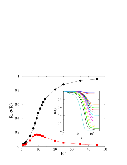
Figure 4: Steady state Kuramoto order parameter in 2d and its variance at $\alpha=3$ at different $K$ values for $L=200$. Inset: $R(t,L=200)$ for $K=$ 1, 2, 3, 5, 7, 8, 9, 10, 11, 12, 13, 14, 20, 25, 35, 45 (bottom to top curves).

As remarked in the Introduction section, we conjecture that the Kuramoto order parameter $R$ exhibits a real discontinuous transition above $d_{l}^{R}>4$, while for $d\leq d_{l}^{R}$ a crossover transition ensues. To verify this conjecture, we estimate the transition point $K^{\prime}_{c}$ and check if it diverges in an infinite system. The crossover transition nature (rather than a real transition) is immediately clear as demonstrated by Fig. 5, in which we see an evident shift of the transition point as the system size is varied. The $\sigma(R)$ also become wider and wider as we increase the size.

Particularly, the inset suggest that the transition point shifts linearly with $L$ in 2d [$K^{\prime}_{c}(L)\propto L$]. Hence the transition points exhibit a power-law growth with exponents, suggesting that $K^{\prime}_{c}(L)\to 0$ as $L\to 0$ and $K^{\prime}_{c}(L)\to\infty$ as $L\to\infty$.

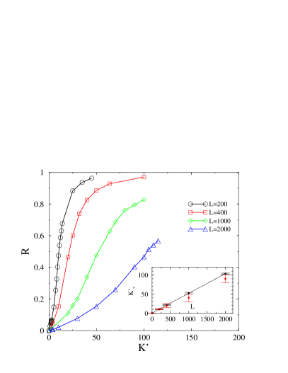
Figure 5: Finite-size behavior of $R$ in 2d for $\alpha=3$ and ordered initial conditions, shows a crossover. Inset: finite-size scaling of $K^{\prime}_{c}$ as estimated by the half values of $R$ (black boxes) and by the $\sigma(R)$ peaks (red bullets) exhibit a linear growth.

For disordered initial conditions we can find much lower steady state values indicated by the inset of Fig.3. The hysteresis loop closes at very large $K$ values only, as was also demonstrated in Ódor et al. (2022) for power-grid networks.

IV Synchronization transition in 3d

In 3d, following the results of the first-order Kuramoto model we expect a real phase transition of the frequency order parameter, but a crossover for the phases. Similarly to 2d we solved the system of equations (1) on large cubic lattices with periodic boundary conditions for linear sizes: $L=50,\,100,\,150,\,200,\,250$ in order to perform finite size analysis.

IV.1 Frequency entrainment phase transition

In case of phase ordered initial states the frequency spread decays with the law $\Omega(t)\propto t^{-d/2}$ above $K_{c}\simeq 1.1$, followed by a finite-size cutoff as shown on Fig. 6 for $L=200$. Doing the finite-size scaling of the transition point, we find that $K_{c}$ does not change within error margins for $L\geq 150$ and we estimate a finite value: $K_{c}=1.15(5)$ as shown in the inset of Fig. 1.

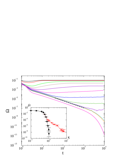
Figure 6: The frequency spread in 3d at $\alpha=3$ for $K=$ 0.1, 0.2, 0.4, 0.5, 0.6, 0.7, 0.8, 0.9, 1, 1.05, 1.1, 2 (top to bottom curves) for $L=200$ linear sized lattices and phase ordered initial conditions. The dashed line marks a numerical fit at the critical point $K_{c}=1.02(2)$ with $t^{-d/2}$. Inset: Steady state values obtained by starting from ordered (black bullets) and disordered (red boxes) initial conditions.

However, in case of the fully random phase initial condition the decay at the critical point seems to deviate from the $t^{-d/2}$ law. It can be be fitted by $\Omega(t)\propto t^{-1.8(1)}$ at $K=K_{c}\simeq 7$ as shown on Fig. 7. Note, that around criticality, in the $t>10^{3}$ region, where finite-size effects emerge, the slope of curves increases, suggesting a nontrivial correction like in case of the first-order Kuramoto model Juhász et al. (2019). Due to the limited computing power, this excludes the possibility to see a crossover towards a $\Omega(t)\propto t^{-d/2}$ asymptotic behavior obtained by the linear approximation. We have investigated this behavior for other levels of randomness in the initial state $\theta_{max}=1,\,1.75,\,1.9$, but found it only at the fully random phase case.

In the case with disordered initial conditions, the level-off of $\Omega(t)$, thus $K_{c}$ also occurs at a much higher couplings, than in the ordered initialization case as the consequence of the phase transition. Therefore, we conjecture a possible different scaling behavior, if any, at the higher $K_{c}$ value. The steady state behavior of $\Omega$ is also shown in the inset of Fig. 6. At first sight it may not suggest a discontinuous transition, but as we applied log-log scales, to observe the rapid changes two branches emerge and we can see the occurrence of a wide hysteresis loop as the consequence of different initial conditions.

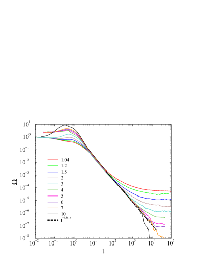
Figure 7: The frequency spread in 3d at $\alpha=3$ for different $K$ values, shown by the legends, for $L=200$ and disordered initial conditions. The dashed line marks a numerical fit at the critical point $K=K_{c}\simeq 7$ with $t^{-1.8(1)}$.

IV.2 Phase order parameter transition

We determined the Kuramoto order parameter values in the steady state for cubes with linear sizes $L=50,100,150,200,150$, using $\alpha=3$ and ordered initial conditions. We display the results for $L=100$ in the Appendix; see Fig. 10. We attempted a finite size scaling analysis as in 2d, as shown on Fig. 8. The $\sigma(R)$ distributions are getting very smeared as $L\to\infty$, making it difficult to locate the peaks. But still, a reasonable power-law fit could be obtained, in agreement with the half value method described in Sec. III.2: $K^{\prime}_{c}\propto L^{0.42(1)}$, as one can see in the inset of Fig. 1. Thus, we still find a crossover behavior in 3d, with a lower $K^{\prime}_{c}$ growth exponent than in 2d, which is expected to decrease as we increase the dimension approaching the lower critical dimension.

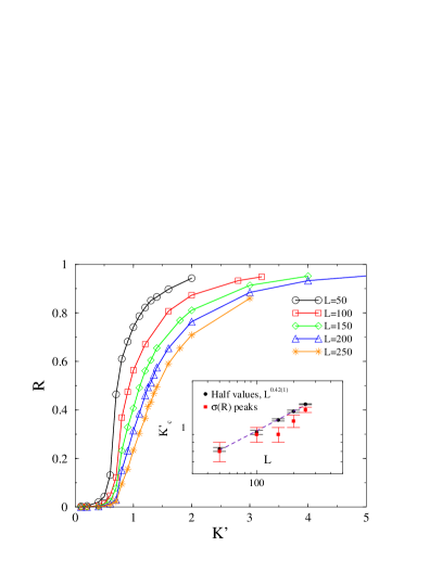
Figure 8: Finite-size behavior of $R$ in 3d for $\alpha=3$ and ordered initial conditions, shows a crossover. Inset: finite-size scaling of $K^{\prime}_{c}$ as estimated by the half values of $R$ (black bullets) as well as by the $\sigma(R)$ peaks (red boxes) exhibit a power-law growth.

V Conclusions

We have performed an extensive numerical study of the synchronization transition of the second-order Kuramoto model in 2 and 3 dimensions. We provided numerical evidence that while the phase order parameter exhibits crossover transition, which diverges with the system size in a power-law manner, the frequency spread order parameter exhibits real phase transition in 3d. In the latter case the finite size dependence of the critical point is negligible on the system sizes we investigated and the transition point for an infinite system, estimated through extrapolation is also very close to those measured in finite systems, except for a logarithmic correction in 2d. The transition of both order parameters exhibit hysteresis behavior though, with the steady state values, which depend on the initial conditions.

However, the variance of $R$, representing chaoticity over initial self frequency choices, has a smeared peak around the crossover point, with growing spread as we increase $L$. This makes the location of the crossover point hard to determine, but we used an alternative method, using half values of $R$, consistent with the peak locations, as a reliable way to obtain it. While the $K^{\prime}_{c}(L)$ grows linearly with $L$ in $2d$, in $3d$ we found a nontrivial power-law dependence: $K^{\prime}_{c}(L)\propto L^{0.42(1)}$.

For the $\Omega$ order parameter we did not find a peak at the critical point, in contrast with the case of the massless Kuramoto model, in agreement with a first-order type phase transition behavior. However, we found asymptotic power-law decay: $\Omega(t)\propto t^{-d/2}$ for $K\geq K_{c}$, which agrees with the linear approximation result. This allowed us to perform a crude finite size scaling of $K_{c}$, which exhibits a logarithmic growth of $K_{c}$ in 2d and a saturation in 3d. Thus, similarly to the massless Kuramoto Hong et al. (2005) we claim $d_{l}^{O}=2$ for the lower critical dimension.

We also found a deviation from the linear approximation law in $d=3$ in case of disordered initial states: $\Omega(t)\propto t^{-1.8}$. This behavior might be the consequence of a slow crossover in time or the nonlinearities due to the phase fluctuations on the upper branch of the frequency order hysteresis curve. This behavior may be observable in real-power grid situations, as we found in Ódor et al. (2022), in case of larger damping factors. For $\alpha=0.4$ this anomalous power-law region is less extended, but this is true for all PL-s we see: the damping factor elongates the scaling regions in agreement with the rescaling invariance of the differential equation, shown in Ódor et al. (2022).

The coexistence of power-law dynamics of $\Omega$ and the hysteresis in the steady sates thus classifies this as a hybrid or mixed type of phase transition, which would be interesting to study further.

Appendix

In this appendix we show results in 2d for the $\Omega(t)$ decay solution in case of disordered initial conditions at $\alpha=0.4$.

Furthermore, we also plot the steady state behavior of $R$ in 3d, for $\alpha=3$, at $L=100$ and ordered initial conditions. One can observe a peak in $\sigma(R)$ at $K\simeq 0.85$, where $R\simeq 0.5$.

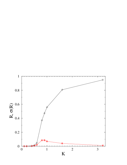
Figure 10: Steady state Kuramoto order parameter and its variance at $\alpha=3$ for different $K$ values for $L=100$. Inset: $R(t,L=100)$.

References

- Pikovsky et al. (2003) A. Pikovsky, J. Kurths, M. Rosenblum, and J. Kurths, Synchronization: A Universal Concept in Nonlinear Sciences, Cambridge Nonlinear Science Series (Cambridge University Press, 2003), ISBN 9780521533522.
- Acebrón et al. (2005) J. A. Acebrón, L. L. Bonilla, C. J. P. Vicente, F. Ritort, and R. Spigler, Rev. Mod. Phys. 77, 137 (2005).
- Arenas et al. (2008) A. Arenas, A. Díaz-Guilera, J. Kurths, Y. Moreno, and C. Zhou, Phys. Rep. 469, 93 (2008).
- Kuramoto (1975) Y. Kuramoto, in Proceedings of the International Symposium on Mathematical Problems in Theoretical Physics, edited by H. Araki (Springer, New York, 1975).
- Ott and Antonsen (2008) E. Ott and T. M. Antonsen, CHAOS 18, 037113 (2008).
- Hong et al. (2007) H. Hong, H. Chaté, H. Park, and L.-H. Tang, Phys. Rev. Lett. 99, 184101 (2007).
- Choi et al. (2013) C. Choi, M. Ha, and B. Kahng, Physical Review E - Statistical, Nonlinear, and Soft Matter Physics 88 (2013).
- Sakaguchi et al. (1987) H. Sakaguchi, S. Shinomoto, and Y. Kuramoto, Prog. Theor. Phys. 77, 1005 (1987).
- Hong et al. (2005) H. Hong, H. Park, and M. Choi, Phys. Rev. E 72, 036217 (2005).
- Juhász et al. (2019) R. Juhász, J. Kelling, and G. Ódor, Journal of Statistical Mechanics: Theory and Experiment 2019, 053403 (2019), URL https://doi.org/10.1088%2F1742-5468%2Fab16c3.
- Filatrella et al. (2008) G. Filatrella, A. H. Nielsen, and N. F. Pedersen, Eur. Phys. J. B 61, 485 (2008).
- Tanaka et al. (1997) H.-A. Tanaka, A. J. Lichtenberg, and O. S., Phys. Rev. Lett. 78, 2104– (1997).
- Ódor and Hartmann (2018) G. Ódor and B. Hartmann, Physical Review E 98, 022305 (2018).
- Villegas et al. (2014) P. Villegas, P. Moretti, and M. A. Munoz, Sci. Rep. 4, 1 (2014).
- Millán et al. (2018) A. P. Millán, J. J. Torres, and G. Bianconi, Sci. Rep. 8, 1 (2018).
- Ódor et al. (2022) G. Ódor, S. Deng, B. Hartmann, and J. Kelling, Phys. Rev. E 106, 034311 (2022), URL https://link.aps.org/doi/10.1103/PhysRevE.106.034311.
- Mermin and Wagner (1966) N. D. Mermin and H. Wagner, Phys. Rev. Lett. 17, 1133 (1966), URL https://link.aps.org/doi/10.1103/PhysRevLett.17.1133.
- Ódor and Hartmann (2020) G. Ódor and B. Hartmann, Entropy 22, 666 (2020).
- Cardy (1981) J. L. Cardy, Journal of Physics A: Mathematical and General 14, 1407 (1981).
- Janssen et al. (2004) H.-K. Janssen, M. Müller, and O. Stenull, Physical Review E 70, 026114 (2004).
- Chan et al. (2015) W. Chan, F. Ghanbarnejad, and P. Grassberger, Nature Physics 11, 936– (2015).
- Gómez-Gardeñes et al. (2011) J. Gómez-Gardeñes, S. Gómez, A. Arenas, and Y. Moreno, Physical Review Letters 106, 128701 (2011).
- Coutinho et al. (2013) B. C. Coutinho, A. V. Goltsev, S. N. Dorogovtsev, and J. F. F. Mendes, Physical Review E 87, 032106 (2013).
- Ódor and de Simoni (2021) G. Ódor and B. de Simoni, Phys. Rev. Res. 3, 013106 (2021).
- Grainger and Stevenson (1994) J. Grainger, J. and D. Stevenson, W., Power system analysis (McGraw-Hill, 1994), ISBN ISBN 978-0-07-061293-8.
- (26) K. Ahnert and M. Mulansky, Boost::odeint, URL https://odeint.com.
- Jeffrey et al. (to be published) K. Jeffrey, S. Deng, L. Barancsuk, B. Hartmann, and G. Ódor (to be published).
- Ódor et al. (2022) G. Ódor, G. Deco, and J. Kelling, Phys. Rev. Research 4, 023057 (2022).
- Ódor et al. (2021) G. Ódor, J. Kelling, and G. Deco, J. Neurocomputing 461, 696 (2021).