Equivariant Networks for Crystal Structures

Abstract

Supervised learning with deep models has tremendous potential for applications in materials science. Recently, graph neural networks have been used in this context, drawing direct inspiration from models for molecules. However, materials are typically much more structured than molecules, which is a feature that these models do not leverage. In this work, we introduce a class of models that are equivariant with respect to crystalline symmetry groups. We do this by defining a generalization of the message passing operations that can be used with more general permutation groups, or that can alternatively be seen as defining an expressive convolution operation on the crystal graph. Empirically, these models achieve competitive results with state-of-the-art on property prediction tasks.

1 Introduction

Deep learning has seen remarkable applications in computational chemistry, both on the side of molecular property prediction and molecule generation. For small molecules, these methods are close to a level of precision that would make them suitable for practical applications [46]. However, less attention has been put to the problem of designing neural network architectures for the larger assemblies of atoms that constitute materials. This is a crucial problem, as deep learning could advantageously complement computationally demanding ab initio simulation methods like DFT [38, 28].

In this paper, we address the problem of designing equivariant layers and use them for supervised learning on materials. We focus on crystals, materials characterized by the ordered arrangement of their atoms in lattices. Crystalline materials are largely present around us and essential in technological applications, as they include a large number of metals, ceramics, and salts, among others [3]. They can be described as the regular repetition of a set of atoms, called the unit cell, in all directions of space. These patterns are analogous to wallpaper patterns, for which the repeated structure is an image. Crystals are characterized by a high degree of symmetry which is fundamental in understanding their physical properties. Consequently, we suggest that equivariant deep learning provides an appropriate framework to design function approximators for crystals.

Graph Neural Networks (GNNs) have recently been proposed for supervised prediction tasks on crystals [54, 70, 12]. We hypothesize here that these models may fall short in exploiting crystal symmetry and that structural information is lost when mapping a crystal structure to a graph. In particular, GNNs are equivariant to the permutation of atoms given as input to the model. This condition is overly restrictive and amounts to forgetting about the ordered nature of a crystal. We propose to use models equivariant to a product of groups $G_{\Lambda}\times S_{C}$, where $G_{\Lambda}$ acts at the level of the Bravais lattice, the underlying periodic grid of the crystal, and $S_{C}$ on the unit cells. We show that our proposed equivariant architecture is more expressive than GNNs on this data structure.

By using the crystal structure, our approach amounts to defining a group-equivariant convolution kernel on the crystal in a way that is completely analogous to convolutional neural networks (CNNs). This convolution is defined on a graph associated with a crystal structure. Our contributions are the following: 1) We derive different equivariant models based on the group-theoretical properties of crystals. 2) We show some of the limitations of GNNs for crystal data and propose an alternative data structure to be used with our architecture. 3) We perform a rigorous analysis, cleaning, and processing of the Materials Project database [33] and share the resulting processed dataset to serve as a benchmark for materials applications. 4) We perform experimental tests of our models on the Materials Project database and report results comparable to or better than baselines.

2 Related works

Equivariant neural networks

It is well known that neural networks have to incorporate inductive biases to be useful in practice [67, 7]. Using models that are invariant or equivariant to the symmetry of the data has proven to be a particularly important inductive bias to promote generalization [8]. The first notable application of this idea was the CNN, for which each convolution layer is equivariant to translation [42]. An alternative parameter-sharing view also appears in early works [57]; while more recent equivariant networks have used both convolutional [13, 40, 15, 19], and parameter-sharing view [51, 24]. A few notable symmetries considered in recent years are rotation in image and volumetric data [13, 68, 65], permutation symmetry in sets [72, 50] and graphs [39, 44], as well as Euclidean [60, 10], and rotational symmetry [14, 2, 21, 55, 23]. In this work, we build on foundational work on hierarchical symmetries [45, 64]

Deep learning for materials

The increasing availability of large materials datasets from high-throughput calculations [18, 33, 36, 47, 31, 11], makes deep learning more and more relevant for materials science. Following the successes of GNNs on molecular data, similar models have been proposed for materials as alternatives to methods based on feature engineering. Note that in what follows, we refer to GNNs in a general sense that includes message passing neural networks (MPNNs) [26].Many variants of GNNs exist [35, 62, 71, 44], the underlying idea being for each node to aggregate features of neighboring nodes in a permutation invariant, or in the case of [39] in an equivariant way. The CGCNN [70] and MEGNet models [12] rely on mapping crystal structures to graphs and applying GNNs to obtain a prediction. For the SchNet model, the correspondence with graphs is less explicit [54], but still present. Other approaches combine permutation equivariance with E(3)-equivariance to design models for molecules and materials [5, 53].

3 Background on crystal symmetry

We first start by introducing some principles of crystallography that will be used to derive our main results. A more comprehensive treatment can also be found in the references [20, 59], whereas basics of group theory are covered in [52] for example.

Lattices

A crystal can be described as the periodic and infinite repetition of a pattern in all directions of space. Crystals are conveniently described using lattices as their underlying structures.

An $n$-dimensional lattice $\Lambda$ can be defined as the set of integral combinations of the linearly independent lattice basis vectors $\mathbf{a}_{i}\in\mathbb{R}^{n}$:

$$\Lambda\doteq\left\{\sum_{i}^{n}{m}_{i}\mathbf{a}_{i}\mid m_{i}\in\mathbb{Z}\right\}.$$ (1)

The lattice is entirely specified by its basis vectors $\mathbf{a}_{i}$. A lattice is associated with a group of translations $T_{\Lambda}$ for which the multiplication rule is addition. This captures the translational symmetry of a crystal. A lattice $\Lambda$ also defines subsets of $\mathbb{R}^{n}$ called unit cells. These subsets have the property of tilling the space when translated by lattice vectors. Of particular importance is the primitive cell $U$ for the basis $\mathbf{a}_{i}$:

$$U\doteq\left\{\sum_{i}^{n}{x}_{i}\mathbf{a}_{i}\mid 0\leq x_{i}<1\right\}.$$ (2)

In a material, the unit cell comprises a set of atomic positions $S=\left\{\left(Z_{i},\mathbf{x}_{i}\right)\mid\mathbf{x}_{i}\in U\right\}$, where the integer $Z_{i}$ is the atomic number and $\mathbf{x}_{i}$ the position of the atom. $S$ can contain an arbitrary number of atoms and must not possess a particular structure. Together with the lattice $\Lambda$, the atomic positions provides a complete description of the crystal structure.

It is often useful to define the concept of a sublattice. A sublattice $\Lambda_{P}$ of $\Lambda$ is a lattice with basis vectors $\mathbf{b}_{i}$ such that $\Lambda_{P}\subset\Lambda$. Correspondingly, the supercell $C_{P}$ is the unit cell associated with the sublattice $\Lambda_{P}$, for which $C_{P}\supset U$. The full lattice is generated by translations of the sublattice by a set of centring vectors $\left\{\mathbf{0}\dots\mathbf{v}_{s}\right\}$. More formally, the sublattice is associated with a normal subgroup $T_{\Lambda_{P}}$ of lattice translations, which specifies a coset decomposition of the original lattice $T_{\Lambda}=\left(\mathbf{0}+T_{\Lambda_{P}}\right)\cup\dots\cup\left(\mathbf{v}_{s}+T_{\Lambda_{P}}\right)$. The centring vectors are coset representatives with respect to that decomposition. It is clear that the centering vectors are also the set of lattice points contained in the supercell $C_{P}$.

Example 3.1 (Graphene).

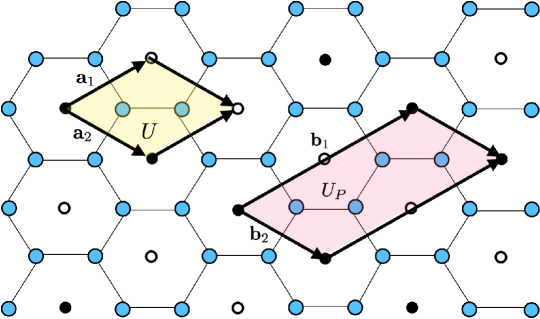
In graphene, carbon atoms are arranged in a two-dimensional crystal with honeycomb structure. The underlying lattice $\Lambda$ has basis vectors $\mathbf{a}_{1}=\frac{a}{2}{\begin{bmatrix}3&\sqrt{3}\end{bmatrix}}$ and $\mathbf{a}_{2}=\frac{a}{2}{\begin{bmatrix}3&-\sqrt{3}\end{bmatrix}}$, where $a$ is a lattice constant. The set of atoms in the unit cell is $S=\left\{\left(6,-\frac{a}{2}{\begin{bmatrix}1&0\end{bmatrix}}\right),\left(6,\frac{a}{2}{\begin{bmatrix}1&0\end{bmatrix}}\right)\right\}$. Figure 1: Graphene crystal structure In Fig.1, blue dots represent carbon atoms. Black and white dots identify points of lattice $\Lambda$ with unit cell $U$. Black points identify a sublattice $\Lambda_{P}$ defined by basis vectors $\mathbf{b}_{1}$ and $\mathbf{b}_{2}$ and with supercell $U_{P}$. The centring vectors $\left\{\mathbf{0},\mathbf{a}_{1}\right\}$ correspond to lattice points contained in the supercell.

Space groups

Symmetry plays a major role in the description of crystals. This symmetry is often directly visible through facets in naturally occurring crystals. Mathematically, it is described by a space group $G$, the set of isometries that maps a crystal structure to itself. As isometries, space groups are subgroups of the Euclidean group $E\left(n\right)$. A space group element can be described as a tuple $\left(\mathbf{W},\mathbf{t}\right)$, where $\mathbf{W}$ is the linear part of the transformation and $\mathbf{t}$ a translation. An element maps a vector $\mathbf{x}\in\mathbb{R}^{n}$ to $\mathbf{W}\mathbf{x}+\mathbf{t}$. The multiplication of space group elements is therefore given by $\left(\mathbf{W}_{1},\mathbf{t}_{1}\right)\left(\mathbf{W}_{2},\mathbf{t}_{2}\right)=\left(\mathbf{W}_{1}\mathbf{W}_{2},\mathbf{W}_{2}\mathbf{t}_{1}+\mathbf{t}_{2}\right)$. The point group $P$ of a space group is the group obtained from linear part operations in $G$, which will in general be rotations and reflections. Considering only elements in $G$ for which the linear part is identity $\left(\mathbf{I},\mathbf{t}\right)$, we obtain the translation subgroup of the space group $T$. It is a normal subgroup, which allows defining the factor group $G/T$ isomorphic to the point group $P$.

The crystallographic restriction theorem guarantees that only certain finite groups are valid point groups of space groups [17]. In particular, in 2 and 3 dimensions, only $n$-fold rotations with $n\in\left\{2,3,4,6\right\}$ are allowed. Two space groups $G$ and $G^{\prime}$ are said to belong to be of same type if they can be related by a change of coordinate system. There are $17$ space group types in 2 dimensions and $230$ in 3 dimensions [59]. For a lattice $\Lambda$, we call the Bravais group of the lattice $P_{\Lambda}$ the set of linear isometries that map $\Lambda$ to itself. Bravais groups provide a way to classify lattices according to their symmetry. We say that two lattices $\Lambda$ and $\Lambda^{\prime}$ belong to the same Bravais type if their Bravais groups are the same matrix groups when written for suitable basis vectors of each lattice. The $5$ Bravais types in 2 dimensions and the $14$ in 3 dimensions are enumerated in the Appendix. The full symmetry group $G_{\Lambda}$ of lattice a $\Lambda$ is given by the semidirect product of its translation group with its Bravais group : $G_{\Lambda}=T_{\Lambda}\rtimes P_{\Lambda}$.

Consider the space group $G$ a crystal structure with lattice $\Lambda$ and unit cell $U$. From the definition of a crystal structure, it is clear that the translation subgroup of $G$ will be $T_{\Lambda}$. However, the point group of $G$ will, in general, not be $P=P_{\Lambda}$. This is because the unit cell may have less symmetry than the underlying lattice, which will result in $P\subseteq P_{\Lambda}$ (see example 3.2). This is the reason why the number of space groups is much larger than the number of Bravais lattices.

Example 3.2 (Wallpaper pattern).

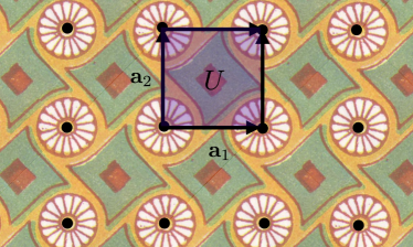
The wallpaper in Figure 2 is described by a square Bravais lattice $\Lambda$ and unit cell $U$ with 4-fold rotational symmetry. The square lattice has a symmetry group $P4m$, with $D_{4}$ Bravais group. However, the unit cell reduces the symmetry of the overall pattern since it does not have reflection axes. The symmetry group of the wallpaper is, therefore, $P4$, with point group $C_{4}$. Figure 2: Egyptian wallpaper [34]

4 Limitations of GNNs

In this section, we examine some of the limitations of GNNs on crystalline data, motivating our model by addressing these limitations. Typical models for crystalline data [70, 12] will build a graph from atoms in the unit cell and assign a feature vector $\mathbf{h}_{i}\in\mathbb{R}^{n}$ to each. Edge features encoding distance might also be used. For convenience, this graph can be represented as a sparse tensor $\mathbf{H}\in\mathbb{R}^{N^{2}\times n}$, where $N$ is the number of atoms considered, and in which node and edge features are encoded on diagonal and off-diagonal entries, respectively. A GNN is a function approximator $f:\mathbb{R}^{N^{2}\times n}\rightarrow\mathbb{Y}$ that produce a prediction, by successive application of layers $\phi\colon\mathbb{R}^{N^{2}\times n_{\ell}}\rightarrow\mathbb{R}^{N^{2}\times n_{\ell+1}}$, where $\ell$ is the layer index.

Expressivity

GNNs are usually stack of layers that are permutation equivariant

$$\phi\left((\mathbf{P}(g)\otimes\mathbf{P}(g))\mathbf{H}\right)=(\mathbf{P}(g)\otimes\mathbf{P}(g))\phi\left(\mathbf{H}\right),\forall g\in S_{N},\mathbf{H}\in\mathbb{R}^{N^{2}\times n},$$ (3)

where $\mathbf{P}(g)$ is the permutation matrix associated with the group element $g$. While $\mathbf{P}(g)$ permutes nodes, $\mathbf{P}(g)\otimes\mathbf{P}(g)$ permutes the vectorized adjacency matrix. Our use of Kronecker product is due to the equality $\text{vec}(\mathbf{P}\mathbf{A}\mathbf{P}^{\top})=(\mathbf{P}\otimes\mathbf{P})\text{vec}(\mathbf{A})$ for $\mathbf{A}\in\mathbb{R}^{N\times N}$.

This captures the fact that these models are designed to be insensitive to node ordering in $\mathbf{H}$. The material is, in a sense, treated as if it was a molecule. Much of the crystal structure is forgotten because it cannot be captured by ordering the nodes in a specific way and is only encoded in positions or distances. We argue that permutation equivariance is an overly strong requirement and was mainly used for practical reasons. When possible, it should be more beneficial to use a model equivariant to the actual symmetry of the data; in this case, the crystal space groups, which will, in general, be much smaller than the symmetric group. Being equivariant to a smaller group results in less restrictive parameter sharing and a more expressive model.

Note that this requirement is different from that of $E(3)$-equivariance characteristic of some architectures [60, 53, 5]. In these models, the $E(n)$ group only acts on the position $\mathbf{x}_{i}\in\mathbb{R}^{3}$ part of each atom’s feature vector. By contrast, the symmetry group of a crystal structure maps the crystal to itself, and its action is a permutation. It therefore offers an alternative to building more powerful architectures for these systems that does not suppose that coordinate information is available. In particular, this approach is more suitable for abstract condensed matter systems, like spin and free-fermion lattice models, in which coordinates are not relevant. Moreover, space groups are subgroups of the Euclidean group; equivariance to space groups is thus less restrictive. In this work, we choose to concentrate on space group equivariance, but we still provide an $E(n)$-equivariant version of our architecture, which is a straightforward extension of [53] in Appendix A.5. Note that equivariance (and not only invariance) is important, as expressive invariant functions can be built by composing equivariant layers with an output pooling layer. Equivariant functions can also be used to predict local properties like magnetization and charge distribution for example.

Invariance and symmetry breaking

Even if the arrangement of atoms in a crystal is symmetric, this does not have to carry over to all local properties of the material. Spontaneous symmetry breaking is common in materials and crucial to describing phenomena such as magnetism and superconductivity [41, 6]. Building a graph only at the unit cell level does not allow to capture local properties that differ across unit cells. Using a supercell of multiple unit cells does not suffice to solve this problem since permutation equivariant models have the property that equal input elements will be mapped to equal outputs elements [58, 73].

5 Input representation

Supercell

Following the arguments of Section 4 we consider the set of atoms in a supercell instead of only in the unit cell, and add explicity symmetry breaking to increase the representational power of the model. Since this increases the computational complexity of the method, we choose to keep the supercells small and define them with sublattice vectors $\mathbf{b}_{i}=2\mathbf{a}_{i}$. The supercell is therefore 8 times larger than the unit cell, with centring vectors $\left\{\sum_{i}^{3}m_{i}\mathbf{a}_{i}\mid m_{i}\in\left\{0,1\right\}\right\}$. For each atom, we build a feature vector with a one-hot encoding of the atomic number and a one-hot encoding identification of the unit cell it belongs to using the corresponding centering vector. We keep track of the index of each atom within the unit cell, and the index of the atoms’ unit cell $\mathbf{h}_{\left(a,i\right)}=\left[\text{onehot}\left(Z_{i}\right),\text{onehot}\left(a\right)\right]$, where $a\in\left\{1,\dots,8\right\}$ and $i\in C$, where $C$ is the number of atoms in the unit cell. The encoding of the unit cell allows to break the symmetry between atoms mapped into each other by lattice translations.

Graph

We construct a graph from atoms in the supercell, encoding relative distances between atoms as edge features. Inspired by [54], an edge feature vector is built from the distance between atoms $d_{ij}=\norm{\mathbf{x}_{i}-\mathbf{x}_{j}}$ as $\mathbf{e}_{ij}=\exp\left(-\gamma\left(d_{ij}-\boldsymbol{\mu}\right)^{2}\right)$. The vector of Gaussian centers $\boldsymbol{\mu}$ and $\gamma$ are hyperparameters. We use this approach to facilitate comparaison to previous works [54, 70], although Bessel encondings [37] could also be considered. It can be seen as “soft" binning of interatomic distances. Using this approach, we use only distance features in contrast to methods that use position vectors. This has the benefit of simplicity while still allowing a complete description of the input structure [66, 4, 63].

Sparsity has proven to be a useful inductive bias in graph representation learning [25], and it is also beneficial in reducing computational complexity. However, atomic bonds are not unambiguously defined in crystals [16, 1]. We choose to follow a similar approach to [32]: an edge is drawn between atoms if they share a Voronoi face and if the distance between atoms is smaller than the sum of atomic Cordero radii plus a cutoff $\Delta=0.5$\mathrm{\SIUnitSymbolAngstrom}$$. This approach has the advantage of being physically sound and producing graphs that are relatively sparse. We provide more details on the graph-building strategy and compute metrics on the resulting graphs in Appendix A.1.

To preserve translational invariance for atoms at the boundary of the supercell, edges are initially also drawn to atoms outside the supercell. Then, if an edge points outside the supercell, its head is mapped to the corresponding representative node inside the supercell. This is analogous to circular padding in image processing.

(a) Identification of the supercell. The sublattice vectors are $\mathbf{b}_{i}=2\mathbf{a}_{i}$

.

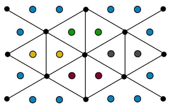
(b) Voronoï tessellation.

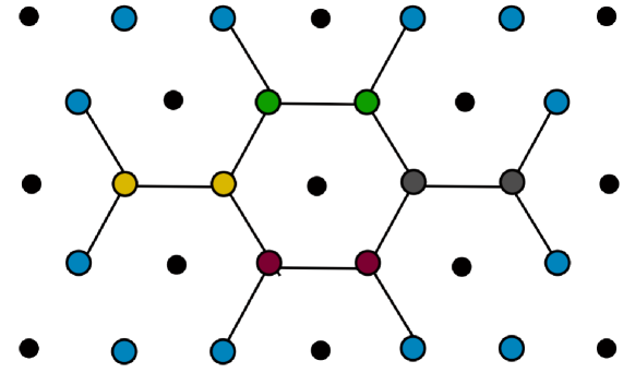
(c) Drawing edges between atoms that share Voronoï faces. The additional condition related to the Cordero radius is not relevant here.

(d) Periodization of the graph. Edges that point to nodes outside the supercell are mapped back to the corresponding atom inside the supercell. Markings show identical atoms.

Figure 3: Building a graph for the graphene crystal structure from Example 3.1.

6 Equivariant crystal networks

Product groups

Consider a crystal structure with space group $G$ and in which each atom has a feature vector $\mathbf{h}_{i}$. Then the space group acts as a permutation of the input atoms

$$g\mathbf{h}_{\left(a,i\right)}=\mathbf{h}_{\left(\pi^{S}_{g}(a),\pi^{U}_{g}(i)\right)}\forall g\in G,$$ (4)

where $\pi^{S}_{g}$ and $\pi^{U}_{g}$ are the permutations associated with group element $g$ on the supercells and within the unit cells respectively.

If a dataset contains only samples that share the same crystal structure, then a model equivariant with respect to $G$ can readily be used. However, the case of a dataset with multiple different crystal structures that would be used in a typical supervised learning setting is more challenging for two reasons. First, samples may have different space groups, which would require different models, each be trained with a fraction of the data. Second, the group action may be different even for the same space group. This is because the unit cells may have different structures and numbers of atoms.

A solution to address these issues is to consider equivariance to a direct product of groups $G_{\Lambda}\times S_{C}$, where the symmetry group of the lattice $G_{\Lambda}$ acts across unit cells and $S_{C}$, the symmetric group, acts within unit cells:

$$(g,h)\mathbf{h}_{\left(a,i\right)}=\mathbf{h}_{\left(\pi^{S}_{g}(a),\pi^{U}_{h}(i)\right)}\forall g\in G_{\Lambda},h\in S_{C}.$$ (5)

In this way, differences in unit cell structures are dealt with by the symmetric group, where parameter-sharing can handle variable-sized inputs [72]. We still have to accommodate 14 different group actions $G_{\Lambda}$ corresponding to the different Bravais lattices. To avoid using a different model for each lattice, we propose two groups to deal with all the lattices. The first option is to consider the least symmetric Bravais lattice of primitive triclinic type and use its symmetry group $P\bar{1}=T_{\Lambda}\rtimes C_{2}$. This group is a subgroup of all the other lattice symmetry groups. The second option we consider is to simply use the symmetric group $S_{\Lambda}$ that is the symmetric group across unit cells, which is an overgroup of all the lattice symmetry groups. This leaves us with a hierarchy of groups, with $S_{N}$, the symmetric group over all atoms of a supercell, being the largest :

$$\underbrace{P\bar{1}\times S_{C}}_{P\bar{1}\text{-model}}\subseteq G_{\Lambda}\times S_{C}\subseteq\underbrace{S_{\Lambda}\times S_{C}}_{S_{\Lambda}\text{-model}}\subseteq S_{N}.$$ (6)

In our experiments, we use the two groups in this hierarchy for different levels of expressivity.

Equivariant message passing

Having defined the group action, we can now build the Equivariant Crystal Network (ECN). We will seek to use the message passing framework, which has demonstrated good performance on molecular data, and generalize it to obtain equivariance to other groups than the symmetric group. The update equations for message passing framework are

$$\mathbf{m}_{ij}=\phi_{e}\left(\mathbf{h}_{i}^{t},\mathbf{h}_{j}^{t},\mathbf{e}_{ij}\right),$$ (7)

$$\mathbf{m}_{i}=\sum_{j\in N_{i}}\mathbf{m}_{ij},$$

$$\mathbf{h}_{i}^{t+1}=\phi_{h}\left(\mathbf{h}_{i}^{t},\mathbf{m}_{i}^{t+1}\right).$$

The idea is to define parameter-sharing patterns for functions $\phi_{e}$ and $\phi_{h}$, such that there can be multiple versions while still retaining equivariance. Following [51], we first define the parameter-sharing pattern of the set of input nodes $\mathbb{N}$, with respect to group $G$ as the colored bipartite graph $\Omega\equiv\left(\mathbb{N},\alpha,\beta\right)$, with the edge-color function $\alpha:\mathbb{N}\times\mathbb{N}\rightarrow\left\{1,\dots,C_{e}\right\}$ and node-color function $\beta:\mathbb{N}\rightarrow\left\{1,\dots,C_{h}\right\}$. We also consider the action of the group $G$ on edges $\Omega$ as $g\cdot\left(i,j\right)\doteq\left(\pi_{g}\left(i\right),\pi_{g}\left(j\right)\right)\forall g\in G$. We define the orbit $G\cdot\left(i,j\right)$ of edge $\left(i,j\right)$ as the set of edges in which it can be moved to by the group action : $G\cdot\left(i,j\right)\doteq\left\{g\cdot\left(i,j\right)\mid g\in G\right\}$. A similar definition applies to the orbit of a node, $G\cdot i\doteq\left\{\pi_{g}\left(i\right)\mid g\in G\right\}$.

We then make the following claim:

Claim 6.1.

The layer defined by the $C_{e}$ functions $\phi^{\alpha\left(i,j\right)}_{e}$ and the $C_{n}$ functions $\phi^{\beta\left(i\right)}_{h}$

$$\mathbf{m}_{ij}=\phi^{\alpha\left(i,j\right)}_{e}\left(\mathbf{h}_{i}^{t},\mathbf{h}_{j}^{t},\mathbf{e}_{ij}\right),$$ (8)

$$\mathbf{m}_{i}=\sum_{j\in N_{i}}\mathbf{m}_{ij},$$ (9)

$$\mathbf{h}_{i}^{t+1}=\phi^{\beta\left(i\right)}_{h}\left(\mathbf{h}_{i}^{t},\mathbf{m}_{i}^{t}\right),$$ (10)

is G-equivariant if the parameter-sharing pattern $\Omega$ respects the equivariance condition:

$$\alpha\left(i,j\right)=\alpha\left(k,l\right) \iff\left(k,l\right)\in G\cdot\left(i,j\right),$$ (11)

$$\beta\left(i\right)=\beta\left(j\right) \iff j\in G\cdot i.$$ (12)

The proof of this claim follows in Appendix A.2. In words, the group action on the graph creates node and edge orbits, and we use a different copy of $\phi_{e}$ and $\phi_{h}$ for each edge and node orbit, respectively. The computational process for producing the pattern is to find the orbit of G-action on the edges (nodes) [51], and the computational cost of this orbit-finding process grows linearly with the number of edges (nodes) [30].

This layer generalizes both MPNNs and equivariant multilayer perceptrons, such as CNNs. The MPNN is recovered with $G=S_{n}$ and a standard CNN with circular convolution with $G=T_{\Lambda}$, $\phi^{\alpha\left(i,j\right)}_{e}\left(\mathbf{h}_{i}^{t},\mathbf{h}_{j}^{t},\mathbf{e}_{ij}\right)=\mathbf{w}^{\alpha\left(i,j\right)}\cdot\mathbf{h}_{i}^{t}$ and $\phi^{\beta\left(i\right)}_{h}\left(\mathbf{h}_{i}^{t},\mathbf{m}_{i}\right)=\text{ReLU}\left(\mathbf{m}_{i}^{t+1}+\mathbf{b}^{\beta\left(i\right)}\right)$

We now consider a product group $G\times H$, acting according to Eq. (5). From Claim 1 of [64], the equivariant linear map for this group is the Kronecker product of equivariant maps for individual groups; see also [45]. The reformulation for parameter-sharing patterns is the following. If parameters-sharing patterns $\Omega_{1}$ and $\Omega_{2}$ satisfy the equivariance condition for $G$ and $H$ respectively, then the parameter-sharing pattern $\Omega=\left({\mathbb{N}\times\mathbb{M}},\alpha,\beta\right)$ satisfies the equivariant condition if

$$\alpha:\mathbb{N}\times\mathbb{M}\times\mathbb{N}\times\mathbb{M}\to\left\{1,\dots,C_{e,1}\right\}\times\left\{1,\dots,C_{e,2}\right\},$$

$$\alpha\left(a,i,b,j\right)=\left(\alpha_{1}\left(a,b\right),\alpha_{2}\left(i,j\right)\right),$$

and

$$\beta:\mathbb{N}\times\mathbb{M}\to\left\{1,\dots,C_{h,1}\right\}\times\left\{1,\dots,C_{h,2}\right\},$$ (13)

$$\beta\left(a,i\right)=\left(\beta_{1}\left(a\right),\beta_{2}\left(i\right)\right).$$ (14)

This simply means that a new color is defined in the product pattern for each possible combination of colors in the original patterns. Example 6.1 demonstrates this idea with a simple example.

We use MLPs to build functions $\phi^{\alpha\left(i,j\right)}_{e}$ and $\phi^{\beta\left(i\right)}_{h}$. The functions used in the experiments are detailed in Appendix A.4. In addition, we add a weighting factor to the edge aggregation 9, as this as been shown to be beneficial by [70, 53]:

$$\mathbf{m}_{i}=\sum_{j\in N_{i}}e_{ij}\mathbf{m}_{ij},\quad\text{where}\quad e_{ij}=\phi_{a}\left(\mathbf{m}_{ij}\right),$$ (15)

and $\phi_{a}$ is simply a linear layer. This change does not affect the equivariance of the model.

Example 6.1.

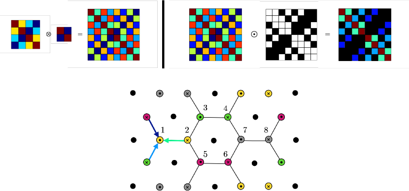
In our running example, the parameter-sharing pattern for the message passing is produced by the Kronecker product of the pattern for the $P2$ group (see Section A.3 for a similar example with the $P6m$ group) and the pattern for the symmetric group $S_{2}$ as shown in the figure below (Top left). However, we only need to keep the colors for which there is a corresponding edge (Top right). Message passing is used on the resulting edge/node colored graph where similar colored nodes and edges use the same functions in message passing. Figure 4: Equivariant message passing for graphene

7 Model implementation

Network architecture

We aimed to keep the architecture of our ECN model as simple as possible. The model receives crystal structure graphs as input, with one-hot encoded feature vectors for each atom. We use 128-dimensional embeddings and keep the same dimension for hidden layers throughout the network. The ECN consists of 6 layers of the equivariant message passing operation 6.1. This is followed by a mean-pooling operation over node embeddings of each graph and a two-layer MLP that outputs the final prediction. Mean pooling is preferred to other options because we only predict intensive physical quantities. These properties are "per-atom" and do not depend on the choice of supercell. Therefore, selecting a pooling operation that respects this invariance makes sense. If we were to predict extensive quantities, sum pooling would be the preferred option.

Input features

Many choices to encode atomic features are possible and have been suggested in the literature. We perform experiments over these variants. For each atom, we encode its type in a feature vector. We consider two strategies, using only information available from the periodic table. The first one is to use only the atomic number. The second one is to use the one-hot encoded group and period numbers for each atom. The second strategy could benefit from promoting better generalization since embeddings of atoms belonging to the same group or period will show a certain similarity. Around $24\%$ of the structures retained in the Materials Project dataset have been computed using the Hubbard-$U$ extension of DFT. Since this information can significantly influence the resulting properties [61] it is added to the atomic feature vector as a binary feature.

Other details

We implemented our model using Pytorch [49]. We use a sparse implementation of the equivariant message-passing based on the Pytorch Scatter package [22]. We use the AdamW optimizer [43] with weight decay regularization. The full hyperparameter setup is provided in Appendix A.7.

8 Experiments

Materials Project

We perform experiments using the Materials Project dataset [33] . This standard dataset of materials informatics comprises more than 120K materials with a complete specification of their crystal structure and some important physical properties obtained with high-throughput DFT calculations.

The Materials Project dataset has not been initially built to serve as a machine learning benchmark; we perform some preprocessing to make it suitable. First, since multiple DFT calculations were sometimes performed on close initial configurations, some samples only show marginal structure differences and resulting properties. This is exemplified by the compound Li9Mn2Co5O16, which appears 322 times in the database. Such duplicates can result in training-test leakage. To prevent this, we consider two structures redundant if they have the same unit cell chemical formula and the same space group. Amongst a set of duplicate structures, the one with the lowest formation energy is chosen. Second, we filter out one-dimensional and two-dimensional materials from the dataset to only keep three-dimensional materials. Finally, we remove materials for which the unit cell contains more than 50 atoms. These are often associated with molecular and inorganic crystals with very different properties than the other materials. Training, validation, and test splits are 80%, 10%, and 10% of the dataset. We provide statistics on the processed dataset in Appendix A.6.

Following previous work, we predict a few relevant energetic properties: the formation energy $E$, the Fermi energy $E_{F}$, and the band gap $E_{g}$ for the subset of insulating materials. We also predict the binary insulator or conductor character material. Finally, we also predict the magnetic moment per atom $M$. This can be seen as a graph regression or classification task. For regression, training is performed using the mean-squared error (MSE) loss function, but we report the mean-absolute error (MAE). For classification, we use the cross-entropy loss function.

Table 1: Results on the Materials Project dataset.

Method Property $E$(eV/atom) $E_{F}$ (eV) $M$ ($\mu_{B}$/atom) $E_{g}$ (eV) Metal precision Nonmetal precision Original CGCNN 0.039 0.363 - 0.388 80% 95% MEGNet 0.028 - - 0.33 78.9% 90.6% SchNet 0.041 - - - - - Ours CGCNN 0.048 $\pm$ 0.0002 0.307 $\pm$ 0.001 0.111 $\pm$ 0.001 0.399 $\pm$ 0.006 81.2% $\pm$ 3.0 86.3% $\pm$ 3.0 MEGNet 0.056 $\pm$ 0.0002 0.365 $\pm$ 0.007 0.110 $\pm$ 0.001 0.434 $\pm$ 0.006 72.1% $\pm$ 3.0 81.6% $\pm$ 4.0 ECN-$P\bar{1}$ 0.052 $\pm$ 0.001 0.303 $\pm$ 0.004 0.108 $\pm$ 0.002 0.44 $\pm$ 0.02 80% $\pm$ 4.0 84% $\pm$ 4.0 ECN-$S_{\Lambda}$ 0.046 ${\pm}$ 0.002 0.281 ${\pm}$ 0.007 0.106 ${\pm}$ 0.002 0.390 ${\pm}$0.02 79.8% $\pm$ 2.0 83.2% $\pm$ 1.0

We compare the results obtained by our models to baselines [54, 70, 12]. Note that because these papers used different training and test splits and preprocessing schemes (even between themselves), our results cannot be directly compared. To alleviate that, we trained our own versions of two of the baselines using our splits and a similar training procedure. We obtain slightly better or comparable results to the baselines on all targets when evaluated on the same splits. The $S_{\Lambda}$ version offers better performance than the $P\bar{1}$ model overall, showing that it is more beneficial to lean on the side of having slightly more symmetry than necessary at the cost of some expressivity. We provide additional results for the model variants in Section A.8. The benefits of the increased expressivity on this task is in the not crucial, which we think can be explained in part by the relatively small size of the Materials Project dataset. In a larger data regime, we expect that the benefit of increased expressivity will outweight the cost in generalization capability.

Perov-5

Finally, we perform experiments using the Perov-5 dataset [9] as provided by [69]. In this dataset, all the materials share the same Perovskite crystal structure. The task considered is the regression of the heat of formation computed through DFT. Results are shown on Table 2.The improvement on this dataset is significantly more important for the proposed model compared to the baselines than on the Materials Project dataset. We hypothesize that the fact that all the structures are shared in this dataset allows the model to specialize more efficiently leading to better generalization.

Method	Property
	Heat All
CGCNN	0.047 $\pm$ 0.000
MEGNet	0.059 $\pm$ 0.006
ECN-$S_{\Lambda}$	0.038 $\bm{\pm}$ 0.004

Table 2: Perov-5 results

Conclusion

We have shown how to leverage crystal symmetry to build more expressive and physically motivated neural networks for materials data. This allows us to obtain a close equivalent of group equivariant convolution on this data structure. These models show excellent accuracy in supervised property prediction, which supports the idea that symmetry is a useful inductive bias. Such models could be used for other tasks on materials such as dynamics prediction, if the dynamics approximately preserves the crystal structure. We also think that these models have significant potential on more abstract condensed matter systems such as spin models and free-fermion models. We have also defined equivariant message passing, a generalization of the MPNN framework that can potentially be used on any data structures for which a group can capture the symmetry in sparse interactions between the basic elements. One limitation of this approach is that it is not clear how to handle structures with different groups without using a larger group like $S_{\Lambda}$. A potential solution is drawing inspiration from the Natural Graph Neural Networks framework introduced in [27]. Another area of future improvement is on the computational efficiency of the equivariant message passing, which does not benefit from optimized algorithms available for convolutions.

Checklist

1. For all authors…

   1. Do the main claims made in the abstract and introduction accurately reflect the paper’s contributions and scope? [Yes] On both the theoretical and experimental side, the paper’s contributions are aligned with the abstract and introduction.

   2. Did you describe the limitations of your work? [Yes] See Conclusion

   3. Did you discuss any potential negative societal impacts of your work? [N/A] We do not think that this is relevant to this work

   4. Have you read the ethics review guidelines and ensured that your paper conforms to them? [Yes]

2. If you are including theoretical results…

   1. Did you state the full set of assumptions of all theoretical results? [Yes] See 6.1 and its proof in the Section A.2

   2. Did you include complete proofs of all theoretical results? [Yes] The only proof is included in Section A.2

3. If you ran experiments…

   1. Did you include the code, data, and instructions needed to reproduce the main experimental results (either in the supplemental material or as a URL)? [Yes] The details needed to reproduce the experiments are included in the supplementary material Section A.7. A link to the relevant code will also be accessible upon publication of the paper.

   2. Did you specify all the training details (e.g., data splits, hyperparameters, how they were chosen)? [Yes] The details needed to reproduce the experiments are included in the supplementary material Section A.7.

   3. Did you report error bars (e.g., with respect to the random seed after running experiments multiple times)? [Yes]

   4. Did you include the total amount of compute and the type of resources used (e.g., type of GPUs, internal cluster, or cloud provider)? [Yes] This is provided in the supplementary material Section A.7

4. If you are using existing assets (e.g., code, data, models) or curating/releasing new assets…

   1. If your work uses existing assets, did you cite the creators? [Yes] See Introduction and Model implementation sections

   2. Did you mention the license of the assets? [Yes] This is mentioned in the supplementary material Section A.6

   3. Did you include any new assets either in the supplemental material or as a URL? [No] The used dataset will be provided upon publication of the paper.

   4. Did you discuss whether and how consent was obtained from people whose data you’re using/curating? [N/A] This is not relevant according to the license of the used assets.

   5. Did you discuss whether the data you are using/curating contains personally identifiable information or offensive content? [N/A] This is not relevant for this paper.

5. If you used crowdsourcing or conducted research with human subjects…

   1. Did you include the full text of instructions given to participants and screenshots, if applicable? [N/A]

   2. Did you describe any potential participant risks, with links to Institutional Review Board (IRB) approvals, if applicable? [N/A]

   3. Did you include the estimated hourly wage paid to participants and the total amount spent on participant compensation? [N/A]

Appendix A Appendix

Table 3: Bravais lattices in $2$ and $3$ dimensions.

Bravais type	Symmetry group	Abstract point group
2 dimensions
Oblique	$P2$	$C_{2}$
Rectangular	$Pmm$	$D_{2}$
Centered rectangular	$Cmm$	$D_{2}$
Square	$P4m$	$D_{4}$
Hexagonal	$P6m$	$D_{6}$
3 dimensions
Primitive triclinic	$P\bar{1}$	$C_{2}$
Primitive monoclinic	$P2/m$	$C_{2h}$
Base-centered monoclinic	$C2/m$	$C_{2h}$
Primitive orthorhombic	$Pmmm$	$D_{2h}$
Base-centered orthorhombic	$Cmmm$	$D_{2h}$
Body-centered orthorhombic	$Immm$	$D_{2h}$
Face-centered orthorhombic	$Fmmm$	$D_{2h}$
Primitive tetragonal	$P4/mmm$	$D_{4h}$
Body-centered tetragonal	$C4/mmm$	$D_{4h}$
Rhombohedral	$R\bar{3}m$	$D_{3d}$
Hexagonal	$P6/mmm$	$D_{6h}$
Primitive cubic	$Pm\bar{3}m$	$O_{h}$
Body-centered cubic	$Im\bar{3}m$	$O_{h}$
Face-centered cubic	$Fm\bar{3}m$	$O_{h}$

A.1 Graph-building strategies

The graphs were built using the IsayevNN class from the pymatgen [48] package. It implements the commonly used Voronoi tessalation to define neighbors. Two atoms are considered bonded if they share a face in the Voronoi tessalation of the supercell and their distance is less than the sum of the atomic Cordero radii (a measure of the atomic radius) plus a cutoff $\Delta=0.5$\mathrm{\SIUnitSymbolAngstrom}$$. This value of the cutoff was increase compared to [32] to reduce the number of disconnected graphs.

We provide statistics for the graphs obtained by the method described in Section 5. A hard cutoff on atomic distances of $6$\mathrm{\SIUnitSymbolAngstrom}$$ is also imposed on atomic distances.

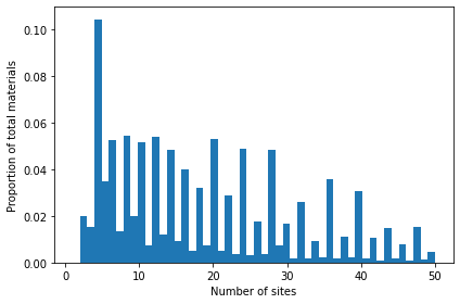
Figure 5: Histogram of the number of primitive cell sites per material in the processed Materials Project dataset.

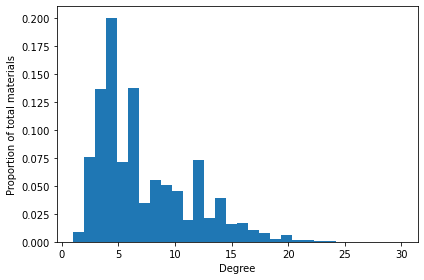
Figure 6: Degree distribution for all graphs.

A.2 Proof of Claim 6.1

We prove that the function defined by

$$\mathbf{m}_{ij}=\phi^{\alpha\left(i,j\right)}_{e}\left(\mathbf{h}_{i}^{t},\mathbf{h}_{j}^{t},\mathbf{e}_{ij}\right),$$ (16)

$$\mathbf{m}_{i}=\sum_{j\in N_{i}}\mathbf{m}_{ij},$$ (17)

$$\mathbf{h}_{i}^{t+1}=\phi^{\beta\left(i\right)}_{h}\left(\mathbf{h}_{i}^{t},\mathbf{m}_{i}^{t}\right),$$ (18)

with

$$\alpha\left(i,j\right)=\alpha\left(k,l\right) \iff\left(k,l\right)\in G\cdot\left(i,j\right),$$ (19)

$$\beta\left(i\right)=\beta\left(j\right) \iff j\in G\cdot i,$$ (20)

is $G$-equivariant by proving the equivariance of every step and using the fact that function composition preserves equivariance.

First, we need to show equivariance of the message function on Equation 16

$$\mathbf{m}_{\pi_{g}(i),\pi_{g}(j)}=\phi^{\alpha\left(i,j\right)}_{e}\left(\mathbf{h}_{\pi_{g}(i)}^{t},\mathbf{h}_{\pi_{g}(j)}^{t},\mathbf{e}_{{\pi_{g}(i)},{\pi_{g}(i)}}\right)\forall g\in G.$$ (21)

Using Equation 19, we have

$$\phi^{\alpha\left(i,j\right)}_{e}\left(\mathbf{h}_{\pi_{g}(i)}^{t},\mathbf{h}_{\pi_{g}(j)}^{t},\mathbf{e}_{{\pi_{g}(i)},{\pi_{g}(i)}}\right)=\phi^{\alpha\left(\pi_{g}(i),\pi_{g}(j)\right)}_{e}\left(\mathbf{h}_{\pi_{g}(i)}^{t},\mathbf{h}_{\pi_{g}(j)}^{t},\mathbf{e}_{{\pi_{g}(i)},{\pi_{g}(i)}}\right)\forall g\in G.$$ (22)

The right-hand side is equal to $\mathbf{m}_{\pi_{g}(i),\pi_{g}(j)}$ by definition.

The message aggregation step at Equation 17 is permutation equivariant

$$\mathbf{m}_{\pi_{g}(i)}=\sum_{\pi_{g}(j)\in N_{\pi_{g}(i)}}\mathbf{m}_{\pi_{g}(i),\pi_{g}(j)}.$$ (23)

Finally, we need to show that the node function on Equation 18 is also equivariant

$$\mathbf{h}_{\pi_{g}(i)}^{t+1}=\phi^{\beta\left(i\right)}_{h}\left(\mathbf{h}_{\pi_{g}(i)}^{t},\mathbf{m}_{\pi_{g}(i)}^{t}\right)\forall g\in G.$$ (24)

Using Equation 20, we find

$$\phi^{\beta\left(i\right)}_{h}\left(\mathbf{h}_{\pi_{g}(i)}^{t},\mathbf{m}_{\pi_{g}(i)}^{t}\right)=\phi^{\beta\left({\pi_{g}(i)}\right)}_{h}\left(\mathbf{h}_{\pi_{g}(i)}^{t},\mathbf{m}_{\pi_{g}(i)}^{t}\right)\forall g\in G.$$ (25)

The right-hand side is equal to $\mathbf{h}_{\pi_{g}(i)}^{t+1}$ by definition.

A.3 Parameter sharing patterns

The parameter sharing patterns are computed using a group-theoretical orbit finding algorithm that has linear complexity in the number of size of the generating sets of a group and in the number of edges in the coloured bipartite graphs [29, 56].

We show the parameter sharing patterns for the different Bravais lattice groups (Figure 7 and Figure 8). For the 2-dimensional groups, we use a $2\times 2$ supercell and for the 3-dimensional groups a $2\times 2\times 2$ supercell. Note that the numbering of the unit cells within the supercell is chosen by convention and can vary for different lattices.

Notice that the parameter-sharing patterns for different groups can be the same. This is because, for different groups, the group action can induce the same orbits on the bipartite graph. In particular, for some groups (Figure 7(c)), the pattern collapses to that of the symmetric group. This can be undesirable since it reduces expressivity. This can be alleviated by using larger supercells or eliminated by considering the group acting on itself instead of on supercells, as done in [13].

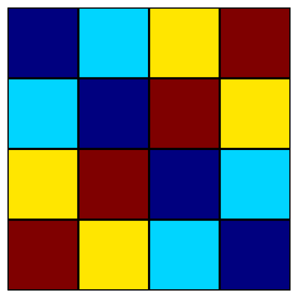
(a) Pattern for groups $P2$ and $Pmm$

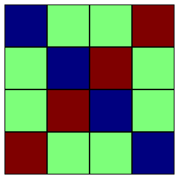
(b) Pattern for group $Cmm$

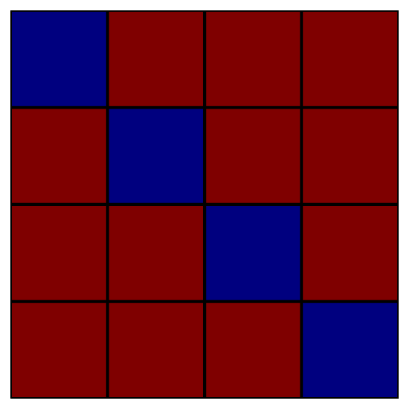
(c) Pattern for groups $P4m$ and $P4m$ and $S_{4}$

Figure 7: Parameter sharing patterns for 2-dimensional Bravais lattices groups

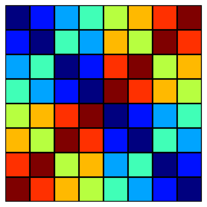
(a) Pattern for group $P\bar{1}$, $P2/m$, $Pmmm$

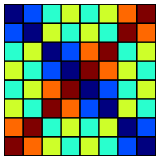
(b) Pattern for group $C2/m$, $Cmmm$, $P4/mmm$

(c) Pattern for group $Immm$

(d) Pattern for group $Fmmm$

(e) Pattern for group $C4/mmm$

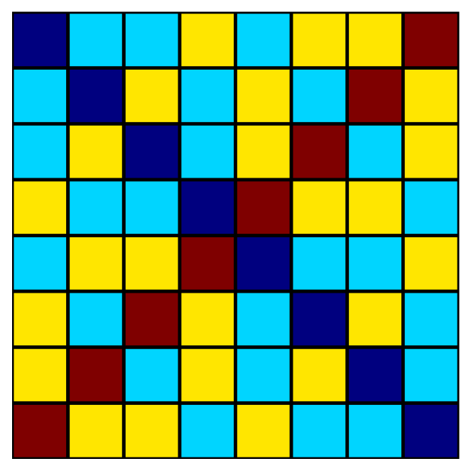
(f) Pattern for group $R\bar{3}m$, $P6/mmm$ and $Pm\bar{3}m$

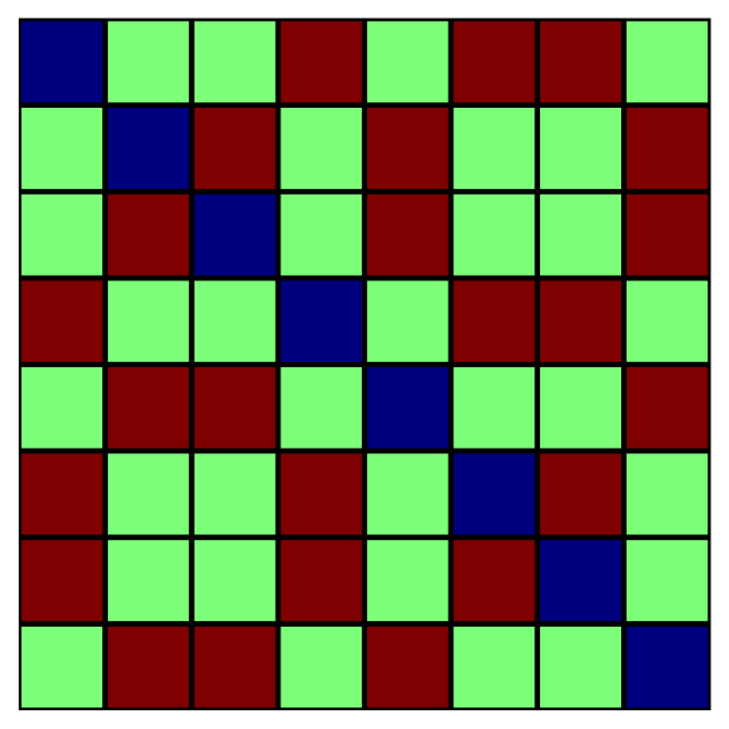
(g) Pattern for group $Im\bar{3}m$

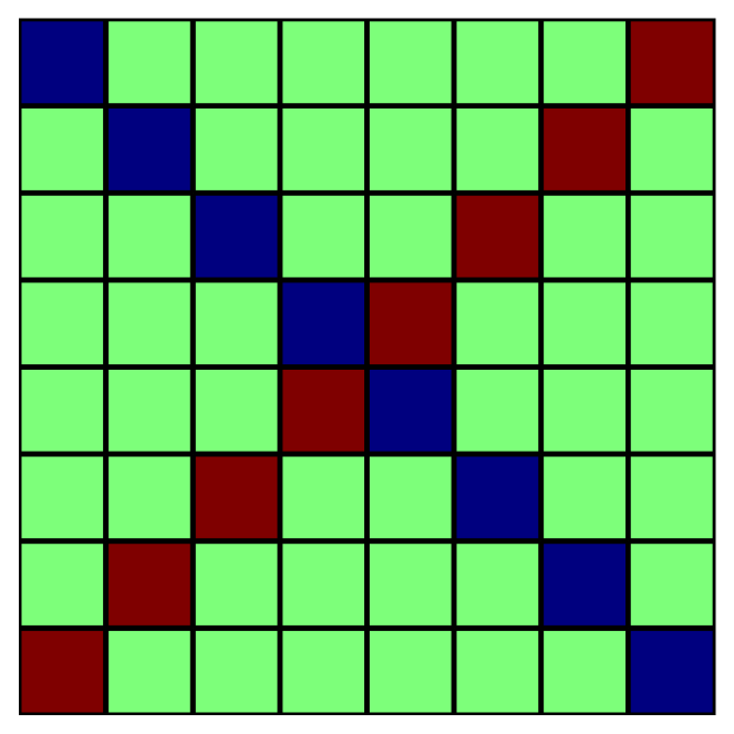
(h) Pattern for group $Fm\bar{3}m$

Figure 8: Parameter sharing patterns for 3-dimensional Bravais lattices groups

A.4 Node and edge functions details

For the node functions $\phi_{h}^{\beta\left(i\right)}$, implementation is facilitated by the fact that for all the group we consider, the group action is transitive. Therefore, for all $i,j\in\mathbb{N}$, $j\in G\cdot i$. This implies that for all $i,j\in\mathbb{N}$, $\beta\left(i\right)=\beta\left(j\right)$. There is thus only one node function, which we implement with two-layer MLP with a residual connection.

For the edge functions $\phi_{h}^{\alpha\left(i,j\right)}$, we do not explicitly build the parameter-sharing patterns. This would be computationally expensive in a dataset in which sample have different unit cell sizes like Materials Project because it would require to build patterns for each unit cell size. Instead, we use an approach inspired by [45]. Let the group be $G_{\Lambda}\times S_{C}$ and each node be represented by the embedding $\mathbf{h}_{\left(a,i\right)}$ where the first index encodes the unit cell within the supercell and the second index encodes the identity of the atom within the unit. Using Theorem 1 of [45], we can define the edge function as

$$\phi_{h}^{\alpha\left(\left(a,i\right),\left(b,j\right)\right)}\left(\mathbf{h}_{\left(b,j\right)}^{t},\mathbf{h}_{\left(b,j\right)}^{t},\mathbf{e}_{\left(a,i\right),\left(b,j\right)}\right)$$ (26)

$$=\delta_{a,b}\phi_{1}^{\alpha_{G_{\Lambda}}\left(i,j\right)}\left(\mathbf{h}_{\left(b,j\right)}^{t},\mathbf{h}_{\left(b,j\right)}^{t},\mathbf{e}_{\left(a,i\right),\left(b,j\right)}\right)+\phi_{2}^{\alpha_{G_{\Lambda}}\left(i,j\right)}\left(\mathbf{h}_{\left(b,j\right)}^{t},\mathbf{h}_{\left(b,j\right)}^{t},\mathbf{e}_{\left(a,i\right),\left(b,j\right)}\right),$$

where $\alpha_{G_{\Lambda}}$ is obtained from the parameter-sharing pattern of the group $\alpha_{G_{\Lambda}}$, which is shared for all the dataset.

In our implementation, $\phi_{1}^{\alpha_{G_{\Lambda}}\left(i,j\right)}$ and $\phi_{2}^{\alpha_{G_{\Lambda}}\left(i,j\right)}$ are built explicitly for as two-layer MLPs for all possible values of $\alpha_{G_{\Lambda}}\left(i,j\right)$.

A.5 ${E(n)}$-equivariant version of ECN

Our architecture can be made ${E(n)}$-equivariant instead of ${E(n)}$-invariant. The basic idea is that multiple edge functions can always be introduced using the parameter sharing pattern. Using a simple generalization of the EGNN model [53], we can define the following layer

$$\mathbf{m}_{ij}=\phi^{\alpha\left(i,j\right)}_{e}\left(\mathbf{h}_{i}^{t},\mathbf{h}_{j}^{t},\norm{\mathbf{x}^{l}_{i}-\mathbf{x}^{l}_{j}},\mathbf{e}_{ij}\right),$$ (27)

$$\mathbf{x}^{l+1}_{i}=\mathbf{x}^{l}_{i}+C\sum_{j\neq i}\left(\mathbf{x}^{l}_{i}-\mathbf{x}^{l}_{j}\right)\phi^{\alpha\left(i,j\right)}_{x}\left(\mathbf{m}_{ij}\right)$$

$$\mathbf{m}_{i}=\sum_{j\in N_{i}}\mathbf{m}_{ij},$$

$$\mathbf{h}_{i}^{t+1}=\phi^{\beta\left(i\right)}_{h}\left(\mathbf{h}_{i}^{t},\mathbf{m}_{i}^{t+1}\right).$$

A.6 Materials Project dataset

We hereafter report the number of samples in the Materials Project dataset at different levels of the preprocessing scheme :

(a)

Full dataset

(b)

No duplicates

(c)

No duplicates and unit cell size constraint

(d)

No duplicates, unit cell size constraint and 3D materials

(e)

No duplicates, unit cell size constraint, 3D materials and valid graphs

(f)

Insulators, no duplicates, unit cell size constraint, 3D materials and valid graphs

Table 4: Number of entries in the Materials Project dataset with processing

(a)	(b)	(c)	(d)	(e)	(f)
126126	114605	96315	82229	78649	33971

We also report the mean and standard deviation of each target for the processed dataset

Table 5: Targets

Property	$E$(eV/atom)	$E_{F}$ (eV)	$M$ ($\mu_{B}$/atom)	$E_{g}$ (eV)
Mean	-1.42	3.77	0.16	2.02
Std. dev.	1.13	2.63	0.44	1.56

A.7 Hyperparameters

We use the same training setup for all the models. The learning rate is initialized at $1\times 10^{-3}$ with a scheduler halving it after each $25$ epoch plateau on the validation loss. Training is perfomed for 1000 epochs or until the learning rate reaches $1\times 10^{-6}$. We performed sweeps over learning rates for all the models to verify that this is indeed a setup in which all models train well.

For the ECN models, we optimized the number of layers, the embedding dimension, the weight decay parameter and dropout (without noticing significant improvement). We use 6 layers of message passing operations. The $\phi^{\alpha\left(i,j\right)}_{e}$ and $\phi^{\beta\left(i\right)}_{h}$ functions are 1-hidden layer MLPs. For the $\phi^{\alpha\left(i,j\right)}_{e}$ functions, the weights for the hidden layer and output layers are shared across all ${\alpha\left(i,j\right)}$. This was found to perform slightly better. The Swish activation function is used. The feature dimension of node embeddings is 100 across all the network. For edge embeddings, the dimension is set at 20.

For the CGCNN model, we used the same embedding sizes (they were not specified in the original paper) and 2 convolution layers. For MEGNet, we used the same architecture setup as in the original paper.

A.8 Supplementary results

Method Property $E$(eV/atom) $E_{F}$ (eV) $M$ ($\mu_{B}$/atom) $E_{g}$ (eV) Metal precision Nonmetal precision ECN-$S_{\Lambda}$ Hubbard 0.052 0.290 0.109 0.368 81.2% 82.9% ECN-$S_{\Lambda}$ Group+Period 0.051 0.295 0.109 0.386 77.6% 85.6%

Table 6: Results for model variants on Materials Project

References

- Alvarez [2013] Alvarez Santiago. A cartography of the van der Waals territories // Dalton Trans. 2013. 42. 8617–8636.
- Anderson et al. [2019] Anderson Brandon, Hy Truong Son, Kondor Risi. Cormorant: Covariant molecular neural networks // Advances in neural information processing systems. 2019. 32.
- Ashcroft et al. [1976] Ashcroft Neil W, Mermin N David, others . Solid state physics. 1976.
- Bartók et al. [2013] Bartók Albert P, Kondor Risi, Csányi Gábor. On representing chemical environments // Physical Review B. 2013. 87, 18. 184115.
- Batzner et al. [2021] Batzner Simon, Musaelian Albert, Sun Lixin, Geiger Mario, Mailoa Jonathan P., Kornbluth Mordechai, Molinari Nicola, Smidt Tess E., Kozinsky Boris. E(3)-Equivariant Graph Neural Networks for Data-Efficient and Accurate Interatomic Potentials. 2021.
- Beekman et al. [2019] Beekman Aron, Rademaker Louk, Wezel Jasper van. An introduction to spontaneous symmetry breaking // SciPost Physics Lecture Notes. 2019. 011.
- Bengio et al. [2013] Bengio Y., Courville A., Vincent P. Representation Learning: A Review and New Perspectives // IEEE Transactions on Pattern Analysis and Machine Intelligence. Aug 2013. 35, 8. 1798–1828.
- Bronstein et al. [2021] Bronstein Michael M, Bruna Joan, Cohen Taco, Veliković Petar. Geometric deep learning: Grids, groups, graphs, geodesics, and gauges // arXiv preprint arXiv:2104.13478. 2021.
- Castelli et al. [2012] Castelli Ivano E, Landis David D, Thygesen Kristian S, Dahl Søren, Chorkendorff Ib, Jaramillo Thomas F, Jacobsen Karsten W. New cubic perovskites for one-and two-photon water splitting using the computational materials repository // Energy & Environmental Science. 2012. 5, 10. 9034–9043.
- Cesa et al. [2021] Cesa Gabriele, Lang Leon, Weiler Maurice. A Program to Build E (N)-Equivariant Steerable CNNs // International Conference on Learning Representations. 2021.
- Chanussot* et al. [2021] Chanussot* Lowik, Das* Abhishek, Goyal* Siddharth, Lavril* Thibaut, Shuaibi* Muhammed, Riviere Morgane, Tran Kevin, Heras-Domingo Javier, Ho Caleb, Hu Weihua, Palizhati Aini, Sriram Anuroop, Wood Brandon, Yoon Junwoong, Parikh Devi, Zitnick C. Lawrence, Ulissi Zachary. Open Catalyst 2020 (OC20) Dataset and Community Challenges // ACS Catalysis. 2021.
- Chen et al. [2019] Chen Chi, Ye Weike, Zuo Yunxing, Zheng Chen, Ong Shyue Ping. Graph Networks as a Universal Machine Learning Framework for Molecules and Crystals // Chemistry of Materials. 2019. 31, 9. 3564–3572.
- Cohen, Welling [2016] Cohen Taco, Welling Max. Group equivariant convolutional networks // International conference on machine learning. 2016. 2990–2999.
- Cohen et al. [2018] Cohen Taco S., Geiger Mario, Köhler Jonas, Welling Max. Spherical CNNs // International Conference on Learning Representations. 2018.
- Cohen et al. [2019] Cohen Taco S, Geiger Mario, Weiler Maurice. A general theory of equivariant cnns on homogeneous spaces // Advances in neural information processing systems. 2019. 32.
- Cordero et al. [2008] Cordero Beatriz, Gómez Verónica, Platero-Prats Ana E., Revés Marc, Echeverría Jorge, Cremades Eduard, Barragán Flavia, Alvarez Santiago. Covalent radii revisited // Dalton Trans. 2008. 2832–2838.
- Coxeter [1961] Coxeter H. S. M. Introduction to geometry. New York: John Wiley & Sons Inc., 1961. xvii+443.
- Curtarolo et al. [2012] Curtarolo Stefano, Setyawan Wahyu, Hart Gus L.W., Jahnatek Michal, Chepulskii Roman V., Taylor Richard H., Wang Shidong, Xue Junkai, Yang Kesong, Levy Ohad, Mehl Michael J., Stokes Harold T., Demchenko Denis O., Morgan Dane. AFLOW: An automatic framework for high-throughput materials discovery // Computational Materials Science. 2012. 58. 218 – 226.
- Dehmamy et al. [2021] Dehmamy Nima, Walters Robin, Liu Yanchen, Wang Dashun, Yu Rose. Automatic Symmetry Discovery with Lie Algebra Convolutional Network // Advances in Neural Information Processing Systems. 2021. 34.
- Dresselhaus et al. [2007] Dresselhaus Mildred S, Dresselhaus Gene, Jorio Ado. Group theory: application to the physics of condensed matter. 2007.
- Esteves et al. [2020] Esteves Carlos, Makadia Ameesh, Daniilidis Kostas. Spin-weighted spherical cnns // Advances in Neural Information Processing Systems. 2020. 33. 8614–8625.
- Fey [2022] Fey Matthias. PyTorch Scatter. 2022.
- Finkelshtein et al. [2022] Finkelshtein Ben, Baskin Chaim, Maron Haggai, Dym Nadav. A simple and universal rotation equivariant point-cloud network // arXiv preprint arXiv:2203.01216. 2022.
- Finzi et al. [2021] Finzi Marc, Welling Max, Wilson Andrew Gordon. A Practical Method for Constructing Equivariant Multilayer Perceptrons for Arbitrary Matrix Groups // arXiv preprint arXiv:2104.09459. 2021.
- Garg et al. [2020] Garg Vikas, Jegelka Stefanie, Jaakkola Tommi. Generalization and representational limits of graph neural networks // International Conference on Machine Learning. 2020. 3419–3430.
- Gilmer et al. [2017] Gilmer Justin, Schoenholz Samuel S., Riley Patrick F., Vinyals Oriol, Dahl George E. Neural Message Passing for Quantum Chemistry // Proceedings of the 34th International Conference on Machine Learning. 70. International Convention Centre, Sydney, Australia: PMLR, 06–11 Aug 2017. 1263–1272. (Proceedings of Machine Learning Research).
- Haan de et al. [2020] Haan Pim de, Cohen Taco S, Welling Max. Natural Graph Networks // Advances in Neural Information Processing Systems. 33. 2020. 3636–3646.
- Hasnip et al. [2014] Hasnip Philip J., Refson Keith, Probert Matt I. J., Yates Jonathan R., Clark Stewart J., Pickard Chris J. Density functional theory in the solid state // Philosophical Transactions of the Royal Society A: Mathematical, Physical and Engineering Sciences. 2014. 372, 2011. 20130270.
- Hiß et al. [2007] Hiß Gerhard, Holt Derek F, Newman Michael F. Computational Group Theory // Oberwolfach Reports. 2007. 3, 3. 1795–1878.
- Holt et al. [2005] Holt Derek F, Eick Bettina, O’Brien Eamonn A. Handbook of computational group theory. 2005.
- Horton et al. [2019] Horton Matthew Kristofer, Montoya Joseph Harold, Liu Miao, Persson Kristin Aslaug. High-throughput prediction of the ground-state collinear magnetic order of inorganic materials using Density Functional Theory // npj Computational Materials. jun 2019. 5, 1.
- Isayev et al. [2017] Isayev Olexandr, Oses Corey, Toher Cormac, Gossett Eric, Curtarolo Stefano, Tropsha Alexander. Universal fragment descriptors for predicting properties of inorganic crystals // Nature Communications. Jun 2017. 8, 1.
- Jain et al. [2013] Jain Anubhav, Ong Shyue Ping, Hautier Geoffroy, Chen Wei, Richards William Davidson, Dacek Stephen, Cholia Shreyas, Gunter Dan, Skinner David, Ceder Gerbrand, al. et. Commentary: The Materials Project: A materials genome approach to accelerating materials innovation // APL Materials. Jul 2013. 1, 1. 011002.
- Jones et al. [1856] Jones Owen, Bedford Francis, Waring J. B., Westwood J. O., Wyatt M. Digby. The Grammar of Ornament. London: Published by Day and Son, Lithographers to the Queen, Gate Street, Lincoln’s Inn Fields, 1856.
- Kipf, Welling [2017] Kipf Thomas N., Welling Max. Semi-Supervised Classification with Graph Convolutional Networks // 5th International Conference on Learning Representations, ICLR 2017, Toulon, France, April 24-26, 2017, Conference Track Proceedings. 2017.
- Kirklin et al. [2015] Kirklin Scott, Saal James E, Meredig Bryce, Thompson Alex, Doak Jeff W, Aykol Muratahan, Rühl Stephan, Wolverton Chris. The Open Quantum Materials Database (OQMD): assessing the accuracy of DFT formation energies // npj Computational Materials. 2015. 1. 15010.
- Klicpera et al. [2020] Klicpera Johannes, Groß Janek, Günnemann Stephan. Directional Message Passing for Molecular Graphs // International Conference on Learning Representations. 2020.
- Kohn, Sham [1965] Kohn W., Sham L. J. Self-Consistent Equations Including Exchange and Correlation Effects // Phys. Rev. Nov 1965. 140. A1133–A1138.
- Kondor et al. [2018] Kondor Risi, Son Hy Truong, Pan Horace, Anderson Brandon, Trivedi Shubhendu. Covariant compositional networks for learning graphs // arXiv preprint arXiv:1801.02144. 2018.
- Kondor, Trivedi [2018] Kondor Risi, Trivedi Shubhendu. On the Generalization of Equivariance and Convolution in Neural Networks to the Action of Compact Groups // Proceedings of the 35th International Conference on Machine Learning. 80. 10–15 Jul 2018. 2747–2755. (Proceedings of Machine Learning Research).
- Landau [1937] Landau Lev Davidovich. On the theory of phase transitions. I. // Phys. Z. Sowjet. 1937. 11. 26.
- LeCun et al. [1995] LeCun Yann, Bengio Yoshua, others . Convolutional networks for images, speech, and time series // The handbook of brain theory and neural networks. 1995. 3361, 10. 1995.
- Loshchilov, Hutter [2019] Loshchilov Ilya, Hutter Frank. Decoupled Weight Decay Regularization // International Conference on Learning Representations. 2019.
- Maron et al. [2019] Maron Haggai, Ben-Hamu Heli, Shamir Nadav, Lipman Yaron. Invariant and Equivariant Graph Networks // International Conference on Learning Representations. 2019.
- Maron et al. [2020] Maron Haggai, Litany Or, Chechik Gal, Fetaya Ethan. On learning sets of symmetric elements // International Conference on Machine Learning. 2020. 6734–6744.
- Noé et al. [2020] Noé Frank, Tkatchenko Alexandre, Müller Klaus-Robert, Clementi Cecilia. Machine Learning for Molecular Simulation // Annual Review of Physical Chemistry. 2020. 71, 1. 361–390. PMID: 32092281.
- O’Mara et al. [2016] O’Mara Jordan, Meredig Bryce, Michel Kyle. Materials Data Infrastructure: A Case Study of the Citrination Platform to Examine Data Import, Storage, and Access // JOM. Jun 2016. 68, 8. 2031–2034.
- Ong et al. [2013] Ong Shyue Ping, Richards William Davidson, Jain Anubhav, Hautier Geoffroy, Kocher Michael, Cholia Shreyas, Gunter Dan, Chevrier Vincent L., Persson Kristin A., Ceder Gerbrand. Python Materials Genomics (pymatgen): A robust, open-source python library for materials analysis // Computational Materials Science. 2013. 68. 314 – 319.
- Paszke et al. [2019] Paszke Adam, Gross Sam, Massa Francisco, Lerer Adam, Bradbury James, Chanan Gregory, Killeen Trevor, Lin Zeming, Gimelshein Natalia, Antiga Luca, others . Pytorch: An imperative style, high-performance deep learning library // Advances in neural information processing systems. 2019. 32. 8026–8037.
- Qi et al. [2017] Qi Charles R, Su Hao, Mo Kaichun, Guibas Leonidas J. Pointnet: Deep learning on point sets for 3d classification and segmentation // Proceedings of the IEEE conference on computer vision and pattern recognition. 2017. 652–660.
- Ravanbakhsh et al. [2017] Ravanbakhsh Siamak, Schneider Jeff G., Póczos Barnabás. Equivariance Through Parameter-Sharing // ICML. 2017. 2892–2901.
- Rotman [2012] Rotman Joseph J. An introduction to the theory of groups. 148. 2012.
- Satorras et al. [2021] Satorras Victor Garcia, Hoogeboom Emiel, Welling Max. E (n) equivariant graph neural networks // arXiv preprint arXiv:2102.09844. 2021.
- Schütt et al. [2017] Schütt Kristof, Kindermans Pieter-Jan, Felix Huziel Enoc Sauceda, Chmiela Stefan, Tkatchenko Alexandre, Müller Klaus-Robert. Schnet: A continuous-filter convolutional neural network for modeling quantum interactions // Advances in Neural Information Processing Systems. 2017. 991–1001.
- Shakerinava, Ravanbakhsh [2021a] Shakerinava Mehran, Ravanbakhsh Siamak. Equivariant Networks for Pixelized Spheres // Proceedings of the 38th International Conference on Machine Learning. 139. 18–24 Jul 2021a. 9477–9488. (Proceedings of Machine Learning Research).
- Shakerinava, Ravanbakhsh [2021b] Shakerinava Mehran, Ravanbakhsh Siamak. Equivariant networks for pixelized spheres // International Conference on Machine Learning. 2021b. 9477–9488.
- Shawe-Taylor [1989] Shawe-Taylor J. Building symmetries into feedforward networks // 1989 First IEE International Conference on Artificial Neural Networks, (Conf. Publ. No. 313). 1989. 158–162.
- Smidt et al. [2021] Smidt Tess E., Geiger Mario, Miller Benjamin Kurt. Finding symmetry breaking order parameters with Euclidean neural networks // Phys. Rev. Research. Jan 2021. 3. L012002.
- Souvignier [2016] Souvignier B. A general introduction to space groups // International Tables for Crystallography. 2016. 1.3, 22–41.
- Thomas et al. [2018] Thomas Nathaniel, Smidt Tess, Kearnes Steven, Yang Lusann, Li Li, Kohlhoff Kai, Riley Patrick. Tensor field networks: Rotation-and translation-equivariant neural networks for 3d point clouds // arXiv preprint arXiv:1802.08219. 2018.
- Tolba et al. [2018] Tolba Sarah A., Gameel Kareem M., Ali Basant A., Almossalami Hossam A., Allam Nageh K. The DFT+U: Approaches, Accuracy, and Applications // Density Functional Calculations. Rijeka: IntechOpen, 2018. 1.
- Veliković et al. [2018] Veliković Petar, Cucurull Guillem, Casanova Arantxa, Romero Adriana, Liò Pietro, Bengio Yoshua. Graph Attention Networks // International Conference on Learning Representations. 2018.
- Villar et al. [2021] Villar Soledad, Hogg David W, Storey-Fisher Kate, Yao Weichi, Blum-Smith Ben. Scalars are universal: Equivariant machine learning, structured like classical physics // Advances in Neural Information Processing Systems. 2021.
- Wang et al. [2020] Wang Renhao, Albooyeh Marjan, Ravanbakhsh Siamak. Equivariant Maps for Hierarchical Structures. 2020.
- Weiler et al. [2018] Weiler Maurice, Geiger Mario, Welling Max, Boomsma Wouter, Cohen Taco. 3d steerable cnns: Learning rotationally equivariant features in volumetric data // Advances in Neural Information Processing Systems. 2018. 10381–10392.
- Weyl [1939] Weyl Hermann. The Classical Groups. 1939.
- Wolpert, Macready [1997] Wolpert D.H., Macready W.G. No free lunch theorems for optimization // IEEE Transactions on Evolutionary Computation. 1997. 1, 1. 67–82.
- Worrall et al. [2017] Worrall Daniel E, Garbin Stephan J, Turmukhambetov Daniyar, Brostow Gabriel J. Harmonic networks: Deep translation and rotation equivariance // Proceedings of the IEEE Conference on Computer Vision and Pattern Recognition. 2017. 5028–5037.
- Xie et al. [2021] Xie Tian, Fu Xiang, Ganea Octavian-Eugen, Barzilay Regina, Jaakkola Tommi. Crystal Diffusion Variational Autoencoder for Periodic Material Generation // arXiv preprint arXiv:2110.06197. 2021.
- Xie, Grossman [2018] Xie Tian, Grossman Jeffrey C. Crystal Graph Convolutional Neural Networks for an Accurate and Interpretable Prediction of Material Properties // Physical Review Letters. Apr 2018. 120, 14.
- Xu et al. [2019] Xu Keyulu, Hu Weihua, Leskovec Jure, Jegelka Stefanie. How Powerful are Graph Neural Networks? // International Conference on Learning Representations. 2019.
- Zaheer et al. [2017] Zaheer Manzil, Kottur Satwik, Ravanbakhsh Siamak, Poczos Barnabas, Salakhutdinov Russ R, Smola Alexander J. Deep Sets // Advances in Neural Information Processing Systems 30. 2017. 3391–3401.
- Zhang et al. [2022] Zhang Yan, Zhang David W, Lacoste-Julien Simon, Burghouts Gertjan J., Snoek Cees G. M. Multiset-Equivariant Set Prediction with Approximate Implicit Differentiation // International Conference on Learning Representations. 2022.