PC-SNN: Supervised Learning with Local Hebbian Synaptic Plasticity based on Predictive Coding in Spiking Neural Networks

Abstract

Deemed as the third generation of neural network, event-driven Spiking Neural Networks(SNNs) combined with bio-plausible local learning rules make it promising to build low-power, neuromorphic hardware for SNNs. However, because of the non-linearity and discrete property of spiking neural networks, the training of SNN remains difficult and is still under discussion. Originated from gradient descent, backpropagation has achieved stunning success in multi-layer SNNs. Nevertheless, it is assumed to lack of biologically plausibility, while consuming relatively high computational resources. In this paper, we propose a novel learning algorithm inspired by predictive coding theory and show that it can perform supervised learning fully autonomously and successfully as the backpropagation, utilizing only local Hebbian plasticity. Furthermore, this method reaches favorable performance compared to the state-of-the-art multi-layer SNNs: test accuracy of 99.25% for Caltech Face/Motorbike dataset, 84.25% for ETH-80 dataset, 98.1% for the MNIST dataset and 98.5% for Neuromorphic dataset: the N-MNIST. Furthermore, our work provides a new perspective on how supervised learning algorithms directly implemented in spiking neural circuitry be conducted, which may give some new insights into Neuromorphological calculation in neuroscience.

I Introduction

Regarded as the third generation neural network, spiking neural networks (SNNs) are made up of bio-inspired spiking neurons [1] and have achieved remarkable performance in pattern recognition tasks [2, 3, 4, 5, 6]. Although SNNs continue to use similar ideas to artificial neural networks (ANNs) when designing network topology, there are essential differences between SNNs and ANNs in the choice of computational neuron model and information encoding strategy. Spiking neurons communicate with each other through binary discrete spikes and they receive and integrate incoming spikes from the presynaptic neurons [7]. Once the membrane potential of a neuron exceeds a pre-defined threshold, emit occurs with an outgoing spike transmitted to the connected neurons in the next layer. Then, the membrane potential is then reset immediately [8]. Since SNNs employ temporal information for transmission as biological neural systems, they can serve as befitting and helpful tools in researching how the brain deals with pattern recognition tasks [9]. In addition, as a result of their unique event-based calculation, SNNs are power-efficient especially for applications with limited computing power such as edge computing, making implementations on neuromorphic chips far from high energy consumption different from these of ANN that are typically dependent on graphics processing units (GPUs) or similar hardware [10].

One of the most challenging component giving rise to the limited applications of SNNs can be attributed to the absence of scalable training algorithms due to complex dynamics and non-differentiable spike function of spiking neural network[10]. Given the main challenge of the non-differentiability of the thresholding activation function of spiking neurons at firing times, the dominant backpropagation mechanism in training ANNs is no longer suited and applicable to SNNs [11]. To overcome these challenges, there are two kinds of supervised learning methodologies have been put forward in the literature. The first type, which is also the most common one, is pre-training ANNs and then adapting the weights obtained to spiking neural networks [12, 13, 14]. Another type of influential works keeps track of the membrane potential of spiking neurons and backpropagates errors based on a final cost function imposing on temporal activities [15, 11, 16, 17]. In this method, the firing time of the neuron is defined as a correlation of its membrane potential or the firing time of presynaptic neurons [18, 19, 20]. SpikeProp [15] is one of the most representative works. However, “dead neuron” problem is observed in those above methods: when a neuron is silent, no learning occurs on it [17]. S4NN [11] has been proposed and solved the “dead neuron” problem effectively: dead neurons that can not be excited in a finite amount of time during the simulation are forced to emit a fake spike at the last time step. At the same time, resetting dead neurons’ synaptic weights to random values sampled from a uniform distribution at the end of each iteration makes it possible for the network to use all neurons’ learning capacity.

In SNN backprop algorithms such as S4NN mentioned above, by backpropagating a global loss function related to activities of output neurons, the gradient value of each synaptic weight during learning is obtained using non-local information that is not directly related to the synapse being modified. In the brain, however, there is no evidence to suggest that this information could be transferred ‘backwards’ throughout the brain [21, 22]. Several researchers believe that the brain tends to execute its learning algorithm locally, depending on just the activity of presynaptic and postsynaptic neurons [23, 24, 25]. Although bio-inspired and local learning rule STDP [10, 26, 27] is often utilized in SNNs, STDP is an unsupervised learning rule and mostly needs an extra classifier, which makes the training process relatively complex and less accurate.

In recent years, nevertheless, aiming to approximate backpropagation in non-spiking MLP models utilizing only biologically plausible connectivity schemes and Hebbian learning rules[28], researchers have come up with a number of models, some of which are discussed as follows. Whittington and Bogacz have shown that the predictive coding framework [29, 30, 31] – A type of biologically feasible and reasonable framework derived from a hierarchical process of probabilistic model – can achieve the same effects as backpropagation in ANNs [23]. It is worth to note that additional nodes are introduced in the predictive coding model to calculate the local prediction error between the value of random variable on a given layer and that evaluated by lower layer. Moreover, these mechanisms in accord with such prediction errors propagation have been observed during perceptual decision tasks [32, 33].

Given that backpropagation in spiking neural networks is not a bio-plausible local learning rule (see section III-D for more details), we intend to apply predictive coding algorithm to SNNs to modify the weights depending on relative timing of spikes and local information between pairs of directly connected neurons, which is locally available. Comparing to the conventional supervised learning algorithms of SNNs, our model trains SNNs with biologically plausible learning principles instead of converting from ANNs or tuning them with BPs to get closer to understanding the brain and have an insight into achieving human-level artificial intelligence.

In this paper, we adapt the predictive coding algorithm, originally designed for ANNs, to spiking neural networks, and we name this model as PC-SNN. In PC-SNN, we use a temporal coding strategy known as First-spike temporal coding, in which neurons fire once at most and the information is encoded in the firing order of priority. We first set forth a spiking neuron probabilistic model in combination with temporal coding. Then we state the inference process in the model, finding the most likely values of random variable of neuron activities in the predictive coding network. Finally we detail how the parameters of the model are updated once the network has reached its steady state. It is worth mentioning that we use simple non-leaky integrate-and-fire (IF) spiking neuron model [34] and fewer hidden neurons in PC-SNN while it reaches a commendable accuracy on both static and dynamic datasets, such as Caltech Face/Motorbike dataset, ETH-80[35], MNIST[36] and N-MNIST dataset[37].

II Related work

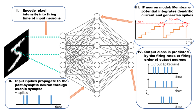
Figure 1: Structure and main procedures of an SNN applying to image classification task. In this example, a simplified fully-connected SNN, with spiking neurons represented as circles and synapses as lines, is shown. (I) The input image is converted with a spike-encoding algorithm. Pixel intensities determine spiking properties of neurons in the input layer, such as firing time of the spike in this work.(II) The pre-synaptic neuron transports spikes across the synapse, which finally accumulate in the dendritic tree of post-synaptic neurons. (III)In the IF neuron model, the neuron membrane potential conbined with the membrane current generates an output spike every time reaching a presumed threshold. Afterwards, the membrane potential will settle at the initial level. (IV) Every output neuron represents a class category. The spike rates or firing times, which are calculated from the emitted spike trains in a predefined time window, are used for class prediction.

Compared with the rapid progress of artificial neural networks in the past few years, SNN training algorithms are an emerging research field in the preliminary stage of fast-growing development. The routine procedure of implementing a classification task on spiking neural network is presented in Fig.1. In general, SNN training algorithms can be divided into Spike Timing Dependent Plasticity (STDP) based localized learning rules[26, 38, 39, 40], ANN-SNN conversion methodologies[41, 42, 43, 44], and spike-based error backpropagation[45, 46, 47]. So far, unsupervised and semi-supervised learning algorithms based on STDP are limited to shallow SNN, and their performance is often inferior to that achieved by artificial neural networks on complex datasets. ANN-SNN transformations produce the best-performing SNN (typically composed of integrated-and-fire (IF) neurons). These neurons are converted by training non-spike ANN(rectilinear Unit (ReLU) as activation function). In order to extend the network more deeply, error backpropagation algorithms based on spikes are proposed for supervised training of SNN.

II-A Spike-based error backpropagation algorithms

Spikeprop[15] is one of the most pioneering and prominent SNN learning algorithm. With a linear approximation of the membrane potential thresholding function, it constructs an mean square error loss function on the basis of the deviations of desired and actual information in the timing of a single spikes, while updating the synaptic weights with a specific SNN-applicable gradient descent. It is one of the most common ways for SNN learning algorithms to define the desired spike times based on timing or firing rates. Mostafa[19] has proposed a feedforward spiking network that implement a temporal coding scheme using spike times as the information preserver, rather than sparse spike counts, and developed a direct training approach that spiking networks do not need to convert from conventional ANNs. By developing a linear and differentiable relation between the timing of spikes on current layer and the timing of spikes on lower layer in the z-domain, any differentiable cost function on the spike times of the network that is verifiable to gradient descent can be imposed.

S4NN[11] is also a new supervised learning rule for multilayer spiking neural networks (SNNs), in which input spike encodes in line with a criterion that spiking latency negatively proportional to the corresponding pixel value. To embody the idea that network is supposed to make rapid and precise decisions with few spikes, a rank-order coding with all neurons firing exactly one spike at most per stimulus is employed. S4NN also proposed relative target firing time to encourage the correct output neuron to fire during the simulation and approximated ReLU with IF neurons.

Recently, an Address event representation (AER) object classification model, which consists of an event-based spatio-temporal feature extraction along with a new segmented probability-maximization (SPA) learning algorithm of SNN, is proposed in [48]. The SPA learning algorithm employs a biologically inspired activation function called Noisy-Softplus relating peak membrane voltage to normalized firing rates. What’s more, by defining and optimizing the probability of the class that the sample actually belongs to, spiking neurons are capable to respond positively to their representative classes. To better capture the peaks of voltage, Peak Detection (PD) mechanism is introduced to orientate information on the time dimension segment by segment to take full advantages of timing information.

II-B Biological plausibility

Spike-based error backpropagation algorithms allow errors to be backpropagated through feedback networks so that the strength/weight of each synapse/connection can be learned/adjusted to eliminate errors. However, since the introduction of the BackPropagation algorithm, researchers have studied whether a similar adaptive mechanism is possible in biological neural systems[49]. Neuroscientists have hold a common view that there is no sign of such backpropagation happening in biological nervous systems[50]. A distinguishing feature of backpropagation algorithms that a specialized feedback network is introduced to backpropagate errors, which is believed nonexistent in the biological neural system. This is because one-to-one correspondence of synapses in the feedforward and feedback networks can not be observed in biological systems. Moreover, considering the fact that in most biological nervous systems, the connection between two neurons is made up of many (or even hundreds) synapses, it is even more unpossible to adapt the corresponding connections in these two networks to be of the same strength in the learning process.

It is shown that the backpropagation algorithm and physical truth in biological neural systems belong to different mechanisms. It is necessary to explore the way in which backpropagation is realized in biology. That is, is there another way to backpropagate errors with no use of a feedback network? In [51], Feng Lin proposed a feedback-network-free B-L algorithm for spiking neural network that is essentially and mathematically indistinguishable from the backpropagation algorithm. The new algorithm inspired by some retrograde regulatory mechanisms is assumed to be realizable in neurons and gets rid of feedback network, which meaningfully enlarges biological plausibility for biological neural networks to learn.

In ANN learning algorithms, a succession of models have been introduced which claim to implement backprop in MLP-style models using only biologically plausible connectivity schemes and Hebbian learning rules. James C.R. Whittington and Rafal Bogacz[23] have shown how the backpropagation algorithm can be closely approximated only utilizing a simple local Hebbian plasticity rule. Specifically speaking, only the activities of presynaptic and postsynaptic neurons directly connected to the synapse modified are involved in learning process. Enlighted by the predictive coding framework[29, 30, 31], the model they proposed confirms the feasibility that this inference could be implemented by biological networks of neurons. A tutorial by Bogacz[52] provides an easy way to discuss in more detail how the model could be implemented in biological neural circuits.

Recently, B. Millidge and A. Tschantz[25] have proved a close correspondence between predictive coding theroy and automatic differentiation across arbitrary computation graphs and produced the desired result on three mainstream machine learning architectures(CNNs, RNNs, and LSTMs), utilizing a predictive coding framework with local learning rules and Hebbian plasticity. Furthermore, Y. Song and T. Lukasiewicz[24] propose a brain learning model that is equivalent to BP while satisfying local plasticity and full autonomy with a fully autonomous Z-IL (Fa-Z-IL) model, which requires no control signal anymore and performs all computations locally, simultaneously, and fully autonomously.

In this paper, we extend these works, showing that predictive coding can not only approximate backprop in MLPs, but can approximate backprop in SNNs while satisfying the following constraints to be considered biologically plausible[52]:

• Local computation: A neuron performs computations only on the basis of the activity of its input neurons and synaptic weights associated with these inputs (rather than information encoded in other parts of the circuit).

• Local plasticity: Synaptic plasticity is only based on the activity of presynaptic and postsynaptic neurons.

III Methods

The notations used in this paper are summarized in Table I and more concrete descriptions are given as the models are introduced.

III-A First-spike temporal coding

Unlike the rate coding where the analog output of an ANN neuron is encoded in the spiking rates of a spiking neuron, we apply a sparser temporal coding strategy with the information enbodied in the firing time. Specifically, neurons can only be activated once at most in a predefined time interval and neurons fire first are thought to be the most active.

In the procedure of encoding the input image to spike trains, denote the $i^{th}$ pixel value of the input grayscale images as $P_{i}$, and the pixel values range in $\left[0,P_{\max}\right]$. The larger the pixel value, the earlier the firing time. In order to inversely convert the pixel value to firing time in range $\left[0,t_{\max}\right]$, we use the following linear transformation formula:

$$t_{i}=\frac{P_{\max}-P_{i}}{P_{\max}}t_{\max}$$ (1)

Subsequently, the input spike trains of the $i^{th}$ pixel (denote input layer as layer 0) can be represented as follows:

$$S_{i}^{0}(t)=\begin{cases}1&\text{ if }t=t_{i}\\ 0&\text{ otherwise }\end{cases}$$ (2)

Indeed, neurons on the following hidden layers and output layer simply integrate weighted incoming spikes over time without leak and emit only one spike right after their membrane potentials cross the threshold for the first time, or being silent if their potentials never reach the threshold. Given that we need to know the firing time of all neurons during the training (see Eq.(14) and (21)), if a neuron does not reach the threshold during training, we artificially set its activation time to $t_{max}$.

III-B Spiking neurons model

We use a non-leaky way to integrate neurons’ potential and stimulate neurons which accumulate receieved spikes from presynaptic neurons through dendritic connection. Each presynaptic spike in integration of its corresponding synaptic weight raises the neuron’s potential. Emission occurs when their internal potentials hit a predefined threshold. The membrane potential of the $j^{th}$ neuron in the $l^{th}$ layer is described by:

$$V_{j}^{l}(t)=\sum_{i}w_{ji}^{l}\sum_{\tau=1}^{t}S_{i}^{l-1}(\tau)$$ (3)

where $w_{ji}^{l}$ signifies the synaptic weight between the $i^{th}$ presynaptic neuron and the $j^{th}$ neuron in $l^{th}$ layer; and $S_{i}^{l-1}(\tau)$ denotes the spike train of the $i^{th}$ presynaptic neuron in layer $l-1$.

If $V_{j}^{l}(t)$ transcends its threshold, then the neuron emits a spike:

$$S_{j}^{l}(t)=\delta\left(t-t_{j}^{l}\right)=\begin{cases}1&\text{ if }V_{j}^{l}(t)\geq\theta_{j}^{l}\&S_{j}^{l}(<t)\neq 1\\ 0&\text{ otherwise }\end{cases}$$ (4)

where $S_{j}^{l}(<t)\neq 1$ makes sure the neurons will not fire until time $t$.

III-C Dynamic target firing time

One of the common methods for setting the target firing time is using fixed firing time: assuming that we have $C$ categories of input images and the label of one input image is $i$, then the target firing time of the $i^{th}$ neuron in the output layer is set to $T_{i}^{o}=\tau$, where $\tau$ is a given constant. The activation time of the remaining output neurons is set to $T_{j}^{o}=t_{\max},1\leq j\leq C,j\neq i$. Although the above setting method is simple and easy to implement, when the actual firing time of the $i^{th}$ neuron $t_{i}^{o}<\tau$, this setting affects the response speed of the network and can not meet our expectation of having the network respond as quickly as possible.

In this paper, we followed the dynamic target firing time proposed by S4NN[11] model which takes the actual activation time into account. Assuming that we feed the image of $i^{th}$ category to the network, the first step is to obtain the actual minimum activation time of the output neuron: $\tau=\min\left\{t_{j}^{o}\mid 1\leq j\leq C\right\}$, then the dynamic target firing time of the $j^{th}$ output neuron is set as follows:

$$T_{j}^{o}=\left\{\begin{array}[]{lll}\tau&\text{ if }j=i&\\ max\{\tau+\gamma,t_{j}^{o}\}&\text{ if }j\neq i\end{array}\right.$$ (5)

In the above dynamic target firing time setting, the output neuron of true category is set to the minimum firing time. $\gamma$ is a positive constant, which ensures the minimum distance between the firing time of true category neuron and that of remaining neurons. Neurons whose activation time is much later than $\tau$ do not change their values.

III-D SNN trained with backpropagation

In order to better show the theoretical advantages on bio-plausibility of PC-SNN compared with BP-SNN, we first review the SNN temporal-coding-based backpropagation algorithm in this section briefly. Firstly, in a $C$-category classification task, a temporal mean square error function is defined as:

$$L=\frac{1}{2}\sum_{j=1}^{C}\left(t_{j}^{o}-T_{j}^{o}\right)^{2}$$ (6)

where $t_{j}^{o}$ and $T_{j}^{o}$ represent the actual and targeted firing time of the $j^{th}$ output neuron respectively. Let’s define an intermediate gradient as $\delta_{j}^{l}=\frac{\partial L}{\partial t_{j}^{l}}$. Therefore backpropagation (BP) updates the weights of the SNN by:

$$\Delta w_{ji}^{l}\!=\!-\!\eta\frac{\partial L}{\partial w_{ji}^{l}}\!=\!-\!\eta\frac{\partial L}{\partial t_{j}^{l}}\frac{\partial t_{j}^{l}}{\partial w_{ji}^{l}}\!=\!-\eta\delta_{j}^{l}\sum_{\tau=1}^{t_{j}^{l}}S_{i}^{l-1}(\tau)$$ (7)

where $\frac{\partial t_{j}^{l}}{\partial w_{ji}^{l}}=\sum_{\tau=1}^{t_{j}^{l}}S_{i}^{l-1}(\tau)$ is formulated detailedly in [11]. The intermediate signal is given as follows:

$$\delta_{j}^{l}\!=\!\left\{\begin{array}[]{cc}t_{i}^{o}-T_{i}^{o}&\text{ if }l\!=\!o\left(i.e.,l\!=\!l_{\max}\right)\\ \sum_{k}\delta_{k}^{l+1}w_{kj}^{l+1}\left[t_{j}^{l}\leq t_{k}^{l+1}\right]&\text{ if }l\!\in\!\left\{1,\ldots,l_{\max}\!-\!1\right\}\end{array}\right.$$

An example of two-layer SNN trained with BP in illustrated in Fig. 2(A). Note that construction of a feedback structure is an essential step to backpropagate the intermediate gradient signal from $\delta_{k}^{l+1}$ to $\delta_{j}^{l}$, indicating that the weights of the feedback network must be brought into correspondence with the feed-forward network.

TABLE I: Notation for BP-SNN and PC-SNN

	Neuron membrane	Membrane threshold	Neuron spike	Firing time activity	Predicted firing time activity	Time interval	Weight	Target firing time	Objective function
BP-SNN	$V_{j}^{l}(t)$	$\vartheta$	$S_{j}^{l}(t)$	$t_{j}^{l}$	$-$	$t_{max}$	$w_{ji}^{l}$	$T_{j}^{o}$	$L$
PC-SNN					$\hat{t}_{j}^{l}$				$F$
	Error node	Intermediate gradient	Local derivative of membrane	Number of layers	Layer size	Minimum firing time of output neurons	Learning rate of weights	Penalizing term
BP-SNN	$-$	$\delta_{j}^{l}$	1	$l_{\max}$	$n^{l}$	$\tau$	$\eta$	$\gamma$
PC-SNN	$\varepsilon_{j}^{(l)}$	$-$	$\alpha$

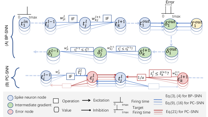
Figure 2: (A):SNN trained with BP. This is a two-layer spiking neural network. Input layer encodes the pixel values into spike trains by temporal encoding. IF neurons in the hidden and output layer transmit information by processing the received spike train and responding to it. Backpropagation compares the actual firing time obtained by the output layer with the target firing time, and propagates the gradient backward layer by layer. As we can see, constructing a feedback structure is an essential step to backpropagate the intermediate gradient signal from $\delta_{k}^{l+1}$ to $\delta_{j}^{l}$, indicating that each weight of the feedback network must be brought into correspondence with the feed-forward network.(B):Predictive coding structure of SNN(PC-SNN). Both Predictions and prediction errors are updated in parallel mode using only local information. Note: Excitation denotes additive operator and Inhibition denotes subtraction operator.

III-E SNN trained with predictive coding framework

In predictive coding framework[30, 31], inference and learning schemes are inspired by EM[53] algorithm, where E-step entails finding the conditional expectation of the causes (i.e. inference) while the M-step identifies the maximum likelihood value of the parameters (i.e. learning). Fig. 2(B) shows a demonstration of a SNN predictive coding model in parallel with the architecture of BP-SNN shown in Fig. 2(A).

III-E1 Probabilistic Model

We regard firing time of IF neurons as random variable in the probabilistic point of view. Let $\textbf{t}^{l-1}$ be a vector of random variables of firing times on layer $l-1$ and $t_{j}^{l}$ be a random variable of firing time of $j^{th}$ neuron in layer $l$. According to design of hierarchical models[30] used in predictive coding, we assume that the random variables on adjacent layers satisfies the following relationships:

$$P\left(t_{j}^{l}\mid\textbf{t}^{l-1}\right)=\mathcal{N}\left(t_{j}^{l};\hat{t}_{j}^{l},\Sigma_{j}^{l}\right)$$ (8)

where the variance $\Sigma_{j}^{l}$ is treated as fixed parameters for simplicity, the mean value of probability density $\hat{t}_{j}^{l}$ is a non-linear function of the activity of lower-layer IF neurons and is determined as the first time when the membrane potential $V_{j}^{l}(t)$ crosses the threshold:

$$V_{j}^{l}(t)=\sum_{i}w_{ji}^{l}\sum_{\tau=1}^{t}\delta\left(\tau-t_{i}^{l-1}\right)$$ (9a)

$$\hat{t}_{j}^{l}=\min\left\{t:V_{j}^{l}(t)>=\vartheta\right\}$$ (9b)

with a constant threshold $\vartheta$ and it is equal for all neurons in this work.

III-E2 Inference

The Inference (i.e. E-step) increases $F$ with respect to the expected cause, ensuring a good approximation to the recognition distribution implied by the network parameters. In the present context, Inference process is to find the most likely neuron activity random variable. Given the inputs, we need to maximize the probability function (see [31] for the technical details):

$$F=P\left(\textbf{t}^{1},\ldots,\textbf{t}^{l_{\max}}\mid\textbf{t}^{0}\right)$$ (10)

to determine the activity of each IF neuron and converge $F$ by iteratively modifying $t_{i}^{l}$ values. To simplify the calculation, we express the probability function $F$ in the form of the logarithm function (because of the monotonicity of the logarithm function, maximizing the logarithm function has the identical impact of maximizing the $F$ function itself):

$$F=\ln\left(P\left(\textbf{t}^{1},\ldots,\textbf{t}^{l_{\max}}\mid\textbf{t}^{0}\right)\right)$$ (11)

Since we assumed that the random variables on one layer depend only on that of previous layer (first order Markov property), we can rewrite the objective function as:

$$F=\sum_{l=1}^{l_{\max}}\ln\left(P\left(\textbf{t}^{l+1}\mid\textbf{t}^{l}\right)\right)$$ (12)

Because the activity of each neuron in one layer is independent of each other, we can write the probability of random variable vector as a product of single random variable probabilities. Substituting Eq.(8) and the expression for a normal distribution into the above equation $F$, we obtain:

$$F=\sum_{l=1}^{l_{\max}}\sum_{j=1}^{n^{l}}\left[\ln\frac{1}{\sqrt{2\pi}\Sigma_{j}^{l}}-\frac{\left(t_{j}^{l}-\hat{t}_{j}^{l}\right)^{2}}{2\Sigma_{j}^{l}}\right]$$ (13)

Then, ignoring constant terms related to the variance, we can organize the objective function as

$$F=-\frac{1}{2}\sum_{l=1}^{l_{\max}}\sum_{j=1}^{n^{l}}\frac{\left(t_{j}^{l}-\hat{t}_{j}^{l}\right)^{2}}{\Sigma_{j}^{l}}.$$ (14)

In consideration of our intention to determine the values $t_{j}^{l}$ that optimize the above objective function, we can attain this goal by modifying $t_{j}^{l}$ proportionally to the gradient with respect to the objective function. In the process of calculating derivative of $F$ over $t_{j}^{l}$, we observe that each $t_{j}^{l}$ influences $F$ in two aspects: it appears in Eq.(14) explicitly, and it also effects the values of $\hat{t}_{k}^{l+1}$ according to Eq.(9a). Thus, the derivative contains two terms:

$$\frac{\partial F}{\partial t_{j}^{l}}=-\frac{t_{j}^{l}-\hat{t}_{j}^{l}}{\Sigma_{j}^{l}}+\sum_{k=1}^{n^{l+1}}\frac{t_{k}^{l+1}-\hat{t}_{k}^{l+1}}{\Sigma_{k}^{l+1}}\cdot\frac{\partial\hat{t}_{k}^{l+1}}{\partial t_{j}^{l}}$$ (15)

Let’s denote

$$\varepsilon_{j}^{l}=({t_{j}^{l}-\hat{t}_{j}^{l}})/{\Sigma_{j}^{l}}$$ (16)

and this error node computes the difference between the current value of $t_{j}^{l}$ and the mean of $\hat{t}_{j}^{l}$ that predicted by the lower layer. Then we have:

$$\frac{\partial F}{\partial t_{j}^{l}}=-\varepsilon_{j}^{l}+\sum_{k=1}^{n^{l+1}}\varepsilon_{k}^{l+1}\cdot\frac{\partial\hat{t}_{k}^{l+1}}{\partial t_{j}^{l}}.$$ (17)

To compute the derivative $\frac{\partial\hat{t}_{k}^{l+1}}{\partial t_{j}^{l}}$, we unfold this term according to chain rule:

$$\frac{\partial\hat{t}_{k}^{l+1}}{\partial t_{j}^{l}}=\frac{\partial\hat{t}_{k}^{l+1}}{\partial V_{k}^{l+1}(t)}\cdot\frac{\partial V_{k}^{l+1}(t)}{\partial t_{j}^{l}}.$$ (18)

For the first factor in Eq.(18), we assume here that for a small enough region around $t=\hat{t}_{k}^{l+1}$, the function $V_{k}^{l+1}(t)$ can be approximated by a linear function of $t$ [15]. We denote the local derivative of $V_{k}^{l+1}(t)$ with respect to $t$ as $\alpha=\frac{\partial V_{k}^{l+1}(t)}{\partial t}$ and it is assumed to be a fixed positive constant in this paper. Because the threshold can only be reached on the rising edge of membrane potential for the first time, thus $V_{k}^{l+1}(t)$ is increasing over $t$ around $t=\hat{t}_{k}^{l+1}$. As for the inverse function, if $V_{k}^{l+1}(t)$ have an increment around $t=\hat{t}_{k}^{l+1}$, it is intuitive that $V_{k}^{l+1}(t)$ will arrive the threshold earlier, and then the value of firing time $\hat{t}_{k}^{l+1}$ will decrease. Thus $\frac{\partial\hat{t}_{k}^{l+1}}{\partial V_{k}^{l+1}(t)}<0$. Considering the derivative of the inverse function $V_{k}^{l+1}(t)$, we approximate $\frac{\partial\hat{t}_{k}^{l+1}}{\partial V_{k}^{l+1}(t)}$ as :

$$\frac{\partial\hat{t}_{k}^{l+1}}{\partial V_{k}^{l+1}(t)}=-\frac{1}{\frac{\partial V_{k}^{l+1}(t)}{\partial t}}=-\frac{1}{\alpha}.$$ (19)

For the second factor in Eq.(18), we note that according to Eq.(9a), reducing $t_{j}^{l}$ will increase $V_{k}^{l+1}(t)$ by $w_{kj}^{l+1}$ earlier in time. Hence we approximate $\frac{\partial V_{k}^{l+1}(t)}{\partial t_{j}^{l}}=-w_{kj}^{l+1}$ if and only if $\left[t_{j}^{l}\leq\hat{t}_{k}^{l+1}\right]$. Substituting the above two derivative terms into Eq.(18), we have

$$\frac{\partial\hat{t}_{k}^{l+1}}{\partial t_{j}^{l}}=\begin{cases}\frac{1}{\alpha}\cdot w_{kj}^{l+1}&\text{ if }t_{j}^{l}\leq\hat{t}_{k}^{l+1}\\ 0&\text{ otherwise }\end{cases}$$ (20)

Finally we obtain the following rule describing changes in $t_{j}^{l}$ over time:

$$\frac{\partial F}{\partial t_{j}^{l}}=-\varepsilon_{j}^{l}+\sum_{k=1}^{n^{l+1}}\varepsilon_{k}^{l+1}\cdot\frac{1}{\alpha}\cdot w_{kj}^{l+1}\left[t_{j}^{l}\leq\hat{t}_{k}^{l+1}\right]$$ (21)

as depicted in Fig. 2(B), and the temporal activity $t_{j}^{l}$ is updated depending only on local nodes and weights.

III-E3 Learning parameters

In the Inference section, the firing time of the neurons on the highest layer are set to the target output firing time, i.e $t_{i}^{o}=T_{i}^{o}$, which is calculated dynamically in section III-C. The values of firing time of all neurons on layer $l\in\left\{1,\ldots,l_{\max}-1\right\}$ are adjusted in the same way as described before (see Eq.(21)). From a neurobiological perspective, both inference and learning are driven in exactly the same way, namely to minimize the free energy $F$[31]. As $w_{kj}^{l+1}$ is modified proportionally to its gradient of the objective function, our network gradually approaches its steady-state. Eventually, the desired output will be predicted when all synaptic weights of the model are updated. We note that $w_{kj}^{l+1}$ affects the value of function $F$ formulated in Eq.(14) by influencing $\hat{t}_{k}^{l+1}$:

$$\frac{\partial F}{\partial w_{kj}^{l+1}}=\frac{t_{k}^{l+1}-\hat{t}_{k}^{l+1}}{\Sigma_{k}^{l+1}}\cdot\frac{\partial\hat{t}_{k}^{l+1}}{\partial w_{kj}^{l+1}}$$

$$=\varepsilon_{k}^{l+1}\cdot\frac{\partial\hat{t}_{k}^{l+1}}{\partial V_{k}^{l+1}(t)}\cdot\frac{\partial V_{k}^{l+1}(t)}{w_{kj}^{l+1}}$$

$$=\varepsilon_{k}^{l+1}\cdot-\frac{1}{\alpha}\cdot\sum_{\tau=1}^{\hat{t}_{k}^{l+1}}S_{j}^{l}(\tau)$$ (22)

where $\sum_{\tau=1}^{\hat{t}_{k}^{l+1}}S_{j}^{l}(\tau)=1$ if $t_{j}^{l}\leq\hat{t}_{k}^{l+1}$ else 0.

The above PC-SNN algorithm has the following properties.

1) According to equation (21) and (III-E3), the change in neuron activity $t_{j}^{l}$ and synaptic weight $w_{kj}^{l+1}$ between layer $l$ and $l+1$ are both proportional to the product of temporal quantities encoded on these two adjacent layers, which can be directly obtained by local connection. Taking $w_{kj}^{1+1}$ as an example shown in Fig. 2(B), the updating of this weight depends only on temporal activities of presynaptic and postsynaptic nodes, i.e., $\varepsilon_{k}^{l+1)}$ and $S_{j}^{l}(t)$, satisfying biologically-plausible local plasticity. This is in contrast to the expression of BP in Eq.(7) and Fig. 2(A), where the weight changes depending on intermediate variables that are passed from the back to the front through a complex function of activities and weights. We refer the changes in Eq.(III-E3) as local Hebbian synaptic plasticity in a manner that the weight change is a simple product of temporal activities of presynaptic and postsynaptic spiking neurons. We use pseudocode to describe the learning and prediction process in Algorithm  1 and  2 respectively.

2) PC-SNN algorithm shows that both the update of spiking temporal activities and weights only utilize the information of nodes directly connected to them, which can be implemented in a parallel manner. This local and parallelizable property of our algorithm may engender a promising prospect of more efficient implementations on neuromorphic hardware and may also facilitate the development of fully distributed neuromorphic architectures.

III-F Algorithm Complexity Analysis

One advantage of using biologically plausible algorithms to train K-layer SNNs is the lower algorithm complexity. Here we use $n$ and $m$ to denote the computational costs of one-step feedforward and one-step local-plasticity propagation, respectively. The PC-SNN finishes the feedforward procedure with $O(nK)$ and then parallelly implements inference process for all hidden layers only using local information. After that, the PC-SNN parallelly updates the network parameters for all hidden layers in a local-plasticity manner. Hence, the algorithm complexity of the PC-SNN is $O(nK+2mK)$. For BP-SNN, besides the feedforward cost with $O(nK)$, it also contains multistep backpropagations layer by layer using differential chain rule, with computing cost of $O(nK+(m+mK)K)$[54].

III-G Analysis of Why PC-SNN Works

According to the EM algorithm[55], assuming that the complete data-set consists of $\mathcal{Z}=(\mathcal{X},\mathcal{Y})$ but that only $\mathcal{X}$ is observed. In the present context, we suppose that an input spike $S^{0}(t)$ and a target firing time $T^{o}$ can be regarded as $\mathcal{X}$, which is given. The $\textbf{t}^{l}$ on layer $l\in\left\{1,\ldots,l_{\max}-1\right\}$ can be regraded as latent variables $\mathcal{Y}$. The complete-data log likelihood is then denoted by $l(\theta;\mathcal{X},\mathcal{Y})$ where $\theta$ is the unknown parameter vector for which we wish to find the Maximum Likelihood Expectation. Here, the $l(\theta;\mathcal{X},\mathcal{Y})$ is actually the objective function $F$ we define in section III-E, which follows the nonlinear model under Gaussian assumptions as Eq.(8). And $\theta$ denotes the whole set of parameters in spiking neural network. :

E-Step: The E-step of the EM algorithm computes the expected value of $l(\theta;\mathcal{X},\mathcal{Y})$ given the observed data $\mathcal{X}$, and the current parameter estimate $\theta_{\text{old }}$ . In particular, we define:

$$F\left(\theta;\theta_{\text{old }}\right) :=\mathrm{E}\left[l(\theta;\mathcal{X},\mathcal{Y})\mid\mathcal{X},\theta_{\text{old }}\right]$$ (23)

$$=\int l(\theta;\mathcal{X},y)p\left(y\mid\mathcal{X},\theta_{old}\right)dy$$

$p\left(\mathcal{Y}\mid\mathcal{X},\theta_{old}\right)$ is the conditional density of $\mathcal{Y}$ given the observed data, $\mathcal{X}$. The goal of E-step is to determine the distribution of $p\left(\mathcal{Y}\mid\mathcal{X},\theta_{old}\right)$, which can also be defined as Gaussian. In the present context of hierarchical Gaussian generative model, we define $p\left(\mathcal{Y}\mid\mathcal{X},\theta_{old}\right)=\prod_{1}^{l_{max}-1}\mathcal{N}\left(\mathcal{Y}^{l};\mu^{l},\sigma^{l}\right),l=1:l_{max}-1$. This intractable posterior can be approximated with variational inference as proved in [25]. The final updating form of neural activities in [25] coincides with maximizing $F\left(\theta;\theta_{\text{old }}\right)$ with respect to $\text{t}^{l}$ in the Inference process, as shown in Eq.(17).

M-Step: The M-step consists of maximizing over $\theta$ the expectation computed in Eq.(23). That is, we set:

$$\theta_{\text{new }}:=\max_{\theta}F\left(\theta;\theta_{\text{old }}\right)$$ (24)

We then set $\theta_{old}=\theta_{new}$. This solution of M-step is shown as the parameters updating in Eq.(III-E3).

The two steps are repeated as necessary until the sequence of $\theta_{new}$’s converges.

1 for all training Data do

2       Temporal coding: $\textbf{S}^{0}\leftarrow\textbf{S}^{input}$;

3       Setting dynamic target firing time: $\textbf{t}^{l_{max}}\leftarrow\textbf{T}^{o}$;

4       while not convergence do

5             Inference:

6            $\varepsilon_{i}^{l}=\frac{t_{i}^{l}-\hat{t}_{i}^{l}}{\Sigma_{i}^{l}}$ ;

7             $\dot{t}_{i}^{l}=-\varepsilon_{i}^{l}+\sum_{j=1}^{n^{l+1}}\varepsilon_{j}^{l+1}\cdot\frac{1}{\alpha}\cdot w_{ji}^{l+1}\left[t_{i}^{l}\leq\hat{t}_{j}^{l+1}\right]$;

8             $t_{i}^{l}\leftarrow t_{i}^{l}+\dot{t}_{i}^{l}$;

9            

10            Update weights:

11            $\dot{w}_{ji}^{l+1}=\varepsilon_{j}^{l+1}\cdot-\frac{1}{\alpha}\cdot\sum_{\tau=1}^{\hat{t}_{j}^{l+1}}S_{i}^{l}(\tau)$;

12             $w_{ji}^{l+1}\leftarrow w_{ji}^{l+1}+\eta\dot{w}_{ji}^{l+1}$;

13            

14       end while

15      

16 end for

Algorithm 1 Learning with predictive coding

1 for all testing Data do

2       Temporal coding: $\textbf{S}^{0}\leftarrow\textbf{S}^{input}$;

3       Forward pass to compute predictions:

4      $V_{j}^{l}(t)=\sum_{i}w_{ji}^{l}\sum_{\tau=1}^{t}S_{i}^{l-1}(\tau)$;

5       ${t}_{j}^{l}=\min\left\{t:V_{j}^{l}(t)>=\vartheta\right\}$;

6      

7 end for

Algorithm 2 Prediction after training

TABLE II: Model parameters for all datasets

Dataset	Model Parameters
	$t_{max}$	$\vartheta$	$\gamma$	$\alpha$	$\eta$	$\Sigma$
Caltech face/motorbike	256	100	8	1	0.1	10
ETH-80	256	100	20	1	0.01	10
MNIST	256	100	20	1	[0.06,0.02]	10
NMNIST	256	100	20	1	0.02	5

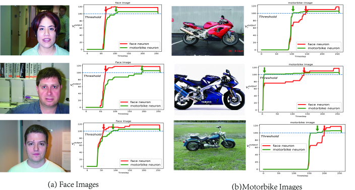
Figure 3: Temporal membrane potentials of output neurons over some Caltech101 face/motorbike images. Arrows indicate the firing time of the corresponding output neuron.

IV Experiments

IV-A Caltech face/motorbike dataset

Caltech101 Face/Motorbike Dataset is a public classification dataset containing a wide variety of faces and motorbikes, which is available at http://www.vision.caltech.edu. Due to the limited experimental data of the original data set, it is decline to overfitting. In the image preprocessing stage, we applied data augmentation to expand the original data set. Specifically, randomly flip the image left to right, add salt and pepper noise, or rotate the image for $\pm 5^{\circ}$ randomly. Through data augmentation, the original 450 face images were expanded to 3600, the original 826 motorbike images were expanded to 3600. And finally 3400 pieces were used as training data and 200 pieces as test data. each image was grayed and resized to $28\times 50$ pixels. Then the rescaled and grayscale image was encoded with first-spike temporal coding and converted into 0/1 spike train.

We performed the analysis with predictive coding spiking neural networks of size 28$\times$50-200-2, in which two output IF neurons represent the face and the motorbike neuron respectively. We randomly initialized the weights of the hidden layer and the output layer to be uniformly distributed in range [0,1] and [0,5]. Although the network will not necessarily converge at that time, we did so to speed up the training. Settings of other hyper parameters are shown in the Table  II.

TABLE III: Classification accuracy of different SNN models on the Caltech face/motorbike dataset along with their learning and classification methods.

Model	Learning Method	Classifier	Accu.(%)
Masquelier et al.(2007)	unsupervised STDP	RBF	99.2
Kheradpisheh et al.(2018)	unsupervised STDP	SVM	99.1
Mozafari et al.(2018)	Reward modulated STDP	Spike-based	98.2
S4NN	backpropagation	Spike-based	99.2
PC-SNN(pro.)	predictive coding	Spike-based	99.25

PC-SNN achieved 99.8% accuracy on the training set and 99.25% accuracy on the test set. These results are superior to the SNN model previously proposed, as shown in Table  III. Note that in the work of Masquelier et al[38] and Kheradpisheh et al[27], models are based on STDP algorithm with multi-layer convolutional layers and extra classifier, like RBF and SVM. S4NN[11] achieved spike-based backpropagation decision making and reached 99.2% accuracy. Our proposed PC-SNN also makes predictions by the spike times and can achieve 99.25% accuracy only by using a two-layer fully- connected network, and more importantly, satisfying local plasticity.

To verify and analyze the functionalities of the proposed PC-SNN, we investigated the membrane potential of output neurons, i.e., $V^{o}_{i}$ after training. As depicted in Fig. 3, we show six sample images and their corresponding output neurons’ membrane potential in the time interval of $[0,t_{max}]$. For every sample image, the target neuron’s membrane potential grows faster and reaches the threshold earlier than that of another neuron. In Fig. 4, we investigated the firing time distribution of the face and motorbike output neurons over 3600 face and 3600 motorbike images at A) the beginning and B) the end of the learning process. As we can see, the firing time of the two output neurons before training was disordered, indicating that the spiking neuron network was not capable of classification at this time. After training, the neuron corresponding to correct category fired significantly earlier than the other.The reason why the firing time of some neurons gathered in $t_{max}$ is as follows: If the neuron is not activated within the predefined time interval, the firing time will be artificially set as $t_{max}$.

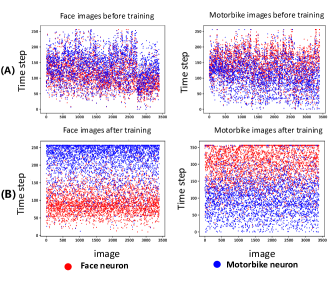
Figure 4: Scatter of firing time of two output neurons on Face/Motorbike images at different stages.(A) Before training;(B) After training.

TABLE IV: MNIST classification performance of recent SNN supervised learning algorithms. Note: E. S. C and I. S. C represent exponential synaptic current and instantaneous synaptic current, respectively.

Model	Coding	Spiking neuron model	Learning rule	Hidden neurons	Accu.(%)
Mostafa (2017)	Temporal	IF (E. S. C)	Temporal Backprop	800	97.2
BP-STDP (2018)	Rate	IF (I. S. C)	Backprop using STDP	1000	96.6
Comsa et al (2019)	Temporal	SRM (E. S. C)	Temporal Backprop	340	97.9
S4NN (2020)	Temporal	IF (I. S. C)	Temporal Backprop	400	98.2
PC-SNN(Pro.)	Temporal	IF (I. S. C)	Predictive coding	200	98.1

IV-B ETH-80 Dataset

TABLE V: Recognition accuracies of the proposed PC-SNN with other methods over the ETH-80 dataset.

Model	Accu.(%)
First-Spike STDP	72.9
Max-Potential STDP	84.5
Convolutional SNN	81.1
Fine-tuned AlexNet	94.2
Supervised DCNN	81.9
SDNN	82.8
PC-SNN(pro.)	84.25

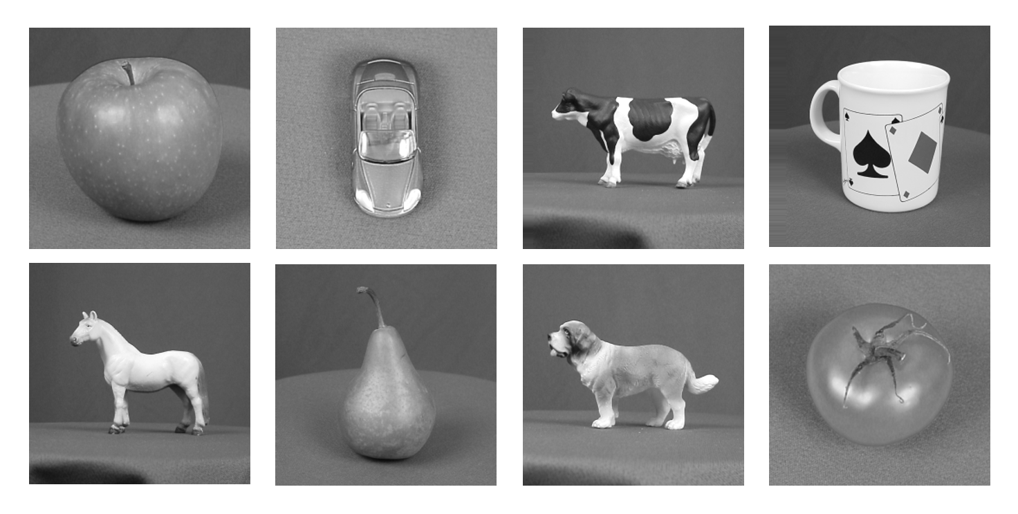
Figure 5: ETH-80: Some sample images of different object categories. The categories of the 8 images are apple, car, toy cow, cup, toy dog, toy horses, pears, and tomatoes respectively.

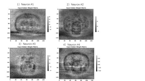
Figure 6: The pattern (input-hidden weight matrix of size 128*128) learned by some of hidden neurons on ETH-80 DATASET. Neurons #1 to #4 correspond to apple, car, cup, and tomato objects respectively.

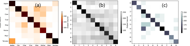
Figure 7: The mean firing time of each output neuron (Y- axis) for different image categories (X-axis) on (a)ETH-80 DATASET, (b)MNIST DATASET and (c)N-MNIST DATASET respectively.

The ETH-80 dataset[35] is consist of various objects of 8 categories: apple, car, toy cow, cup, toy dog, toy horses, pears, and tomatoes (10 instances per category). Each instance was captured from 41 different perspectives. Fig 5 lists some examples of the dataset. ETH-80 is regarded as a standard benchmark showing whether our proposed PC-SNN can solve multi-object classification tasks characterized by high inter-instance variability and handle large view changes. We randomly selected 5 instances for each category as training data, with the remaining 5 instances as test data. Before training, each image was resized to 128*128 grayscale image. We used a network with a hidden layer of 200 neurons which is architecturally analogical to the one used for Caltech face/motorbike dataset.

The recognition accuracy of the proposed PC-SNN along with some other models on the ETH-80 dataset are presented in Table  V. First-spike STDP with a convolutional structure and SVM classifier achieved 72.9%, while Max-Potential STDP using the same convolutional structure and KNN classifier reached accuracy of 84.5%[56]. SNN with convolutional structure[57], an expansion of the Masquelier et al.[38], utilizes 1200 visual features and linear SVM classifier on the trainable layer. In [27], in order to further make use of the feature extraction capability of convolutional neural network, the decision layer of ImageNet-pretrained AlexNet was replaced by an eight-neuron FC layer and trained with the stochastic gradient descent. Considering that the AlexNet model pre-trained on ImageNet has been prepared with a relative strong feature recognition ability, it’s not a fair comparison. A supervised DCNN trained on the gray-scaled images of ETH-80 using the backpropagation algorithm reached the accuracy of 81.9%. SDNN[27] is a deep SNN, comprising several convolutional (trainable with STDP) and pooling layers, achieved 82.8% on ETH-80. Our proposed PC-SNN achieves an accuracy of 84.25% using only two fully-connected layers, which is at the same level as the best results of current SNN learning strategies, which proved that PC-SNN can recognize objects with high precision and bio-plausibility.

Fig. 7(a) shows the mean firing time of each output neuron on images of different obeject categories. As we can see, for each category, the correct neuron shows a far smaller mean firing time in comparison to other neurons. Object ‘tomato’ has the minimum mean firing time of 141, while ‘toy horse’ has the maximum mean firing time of 210. The gap of mean firing time between dogs, horses, and cows neurons are relatively small, which can be attributed to the overall shape similarity and miscategorization between these object categories. Fig. 6 demonstrates the input-hidden weight matrix of some neurons on hidden layer. Comparing with the real ETH-80 images in Fig. 5, Neuron #1 to #4 all have learned a combination of object features, while their preferred features correspond to apple, car, cup and tomato respectively. Toy cow, dog and horse have a relatively complex shapes, indicating why the learned features of them are not visually well detectable.

IV-C MNIST Dataset

MNIST dataset[36] consists of 60000 training images and 10000 test images, each of which is a 0-9 handwritten digit with a size of 28$\times$28 pixels. We conducted the analysis on PC-SNN of size 28$\times$28-200-10. The synapse weights of two layers were randomly initialized from uniform distribution range in [0,5] and [0,10] severally. We also applied dropout in hidden layer to randomly deactivate half of the hidden neurons, which effectively reduced overfitting and slightly raised training accuracy.

Fig 8 shows the learning curves for two different algorithms: predictive coding SNN proposed in this paper and backpropagation SNN proposed in S4NN [11], which is a supervised temporally-backpropagation algorithm and reached state-of-the-art performance with fully-connected multi-layer SNN. It’s easy to see that predictive coding algorithm performs comparably to backpropagation in spiking neural networks in a similar behavior through the epochs. The classification accuracy of our model for MNIST classification is listed in Table IV along with other supervised learning method [19, 58, 59, 11] of spiking neural networks. This comparison strengthens the feasibility of the bio-inspired PC-SNN algorithm applied to fully connected SNN architecture with temporal coding. The advantages of our proposed PC-SNN lie in our comparable performance (98.1% categorization accuracy) to other conventional supervised learning methods while only using end-to-end, bio-plausible and local rules. Moreover, our model used simple IF neuron with an instantaneous synaptic current, one-spike-at-most temporal coding and only 200 neurons in the hidden layer which improved network computing efficiency.

Fig. 7(b) shows the mean firing time of output neurons for all kinds of handwritten digits categories. For each category of handwritten digits, the target neurons fire much earlier than the others. According to the gray level of the color map, we can see the gap between the mean firing time of correct output neuron and other neurons. Considering our classification criterion of “the first neuron to fire implies prediction”, our algorithm achieved accurate prediction for all categories of handwritten digital images. Fig. 9 shows the firing time distribution of winner neuron (earliest activated neuron regardless of its category) and non-winner neuron respectively. As illustrated, about 90% of winner neurons activate before 150 timesteps, and the average firing time is 60 timesteps. About 85% of non-winner neuron is fired after 150 timesteps and the mean firing time is 234. This means that the firing time distribution of winner neuron and non-winner neuron is clearly divided, which is conducive to network training and judgment. It’s also denoted that there is about a 50-percent chance that PC-SNN can respond to input images within about 60 timesteps.

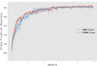
Figure 8: Comparison of learning curves for our proposed PC-SNN and backpropagation (BP-SNN) on the MNIST dataset.

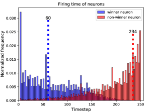
Figure 9: The histogram of the firing time for the winner neurons(blue bar) and non-winner neurons(red bar) over the training images. The dashed line indicates the mean firing time of the winner(non-winner) neuron.

IV-D N-MNIST Dataset

The Neuromorphic-MNIST (N-MNIST) dataset[37], a spiking version of the well-known frame-based MNIST dataset, is designed specifically for spiking neural networks and consists of the same 60000 training samples and 10000 testing samples as the original benchmark. The N-MNIST dataset was collected by mounting the ATIS sensor on a motorized translation unit and moving the sensor while viewing the MNIST example on the LCD. Each dataset sample is 300 ms long and 34×34 pixels big. Different from MNIST data shape $(X,Y)$, the data shape of each input spike of N-MNIST is $(P,X,Y,T)$, where $P$ represents the polarity of the event (positive when the pixel brightness increases, negative when the brightness decreases); $X=Y=34$ is the visual scale; In this work, we set time interval $T$ to 256ms. Fig. 10 shows the visualization of an event stream representing a sample of Digit ‘5’ in N-MNIST dataset.

The results on NMNIST classification listed in Table  VI show that PC-SNN learning algorithm reaches the current state of the art result on NMNIST dataset. Lee et al.[60] generated a continuous and differentiable signal on which gradient descent can work and achieved a high accuracy of 98.66%, in which the spike signal after low pass filtering is added to the membrane potential to deal with the abrupt change of membrane potential. The SKIM[61] is a neural synthesis technique producing networks of neurons and synapses, where arbitrary functions are implemented on spike-based inputs. Our model outperforms SKIM by a margin of 6%. In SLAYER[17], a CUDA accelerated framework to train SNNs was generated, which handled the non-differentiable nature of the spike function and reached state of the art accuracy of 98.89% in fully-connected spiking neural network. Liu et al.[48] introduce a segmented probability-maximization and peak detection algorithm to deal with AER object classification task and reached an accuracy of 96.3%. We conducted experiments on three network structures, and our model gets the classification accuracy of 97.5% on a 2-layer spiking neural network with 500 hidden neurons, 97.8% with 800 hidden neurons and 98.5% with a 3-layer architecture. It is worth mentioning that we use simpler IF neuron model and time-to-first-spike coding to achieve local learning in spiking neural network comparing to other supervised methods. Fig. 7(c) illustrates the mean firing time of output neurons for different digit categories of N-MNIST dataset. Our proposed PC-SNN, using neurons pre-assigned to the class labels, successfully found task-specific diagnostic features. That is because: each neuron, assigned to a certain class, behaves ideally by responding early for the instances belonging to the target class. The average firing time of digit ‘2’ input images is 134, which is the minimum among the 10 categories. And the maximum average activation time is 215, corresponding to the digit ‘8’.

The accuracy and MSSE curves achieved by PC-SNN on N-MNIST dataset are depicted in Fig. 11. From the comparison of the three architectures, it can be seen that the relatively simple structure 34*34*2-500-10 can achieve a high accuracy within 40 epochs and quickly converge to 97.5% accuracy, and 34*34*2-800-10 also has a similar performance. The accuracy of the 3-layer network structure 34*34*2-500-500-10 is relatively low in the initial stage, but converges to 98.5% after 80 epochs. The reasons for the above results may be that: although the 3-layer network has better feature extraction ability and its final convergence accuracy is superior to that of the 2-layer network, the simpler 2-layer network has a smaller number of parameters and is easier to train and converge, while the deeper network has a larger amount of parameters and requires more iterations to achieve convergence. Fig. 11(2) shows the MSSE curves of error nodes on the output layer after the inference process of each epoch. Corresponding to the accuracy curves as Fig. 11(1), MSSE gradually decreased along with the epoches and finally converged close to 0, indicating that with the training of network, inference is able to better predict the activity of neuron nodes and conform to local plasticity.

TABLE VI: Comparison of classification accuracy on N-MNIST dataset.Note: E. S. C and I. S. C represent exponential synaptic current and instantaneous synaptic current, respectively.

Model	Coding	Spiking neuron model	Learning rule	Architecture	Accu.(%)
Lee et al.	Rate	LIF(E.S.C)	Spike-based Backprop	34*34*2-800-10	98.66
SKIM	Temporal	–	Synaptic Kernel Inverse	34*34*2-10000-10	92.87
SLAYER	Rate	SRM(E.S.C)	Spike-based Backprop	34*34*2-500-500-10	98.89
SPA	Rate	LIF(E.S.C)	Probability-maximization	HMAX-S1-C1-FC	96.3
PC-SNN(pro.)	Temporal	IF(I.S.C)	Predictive coding	34*34*2-500-10	97.5
PC-SNN(pro.)	Temporal	IF(I.S.C)	Predictive coding	34*34*2-800-10	97.8
PC-SNN(pro.)	Temporal	IF(I.S.C)	Predictive coding	34*34*2-500-500-10	98.5

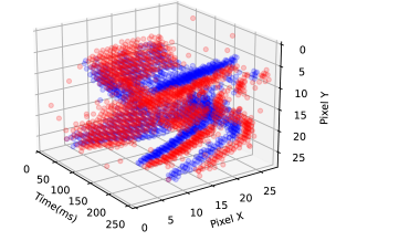
Figure 10: Visualization of the ATIS event stream representing the Digit ‘5’ in N-MNIST dataset. ON and OFF events are represented by red and blue circles respectively.

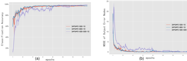
Figure 11: (a)Classification accuracy and (b)Mean-sum-of-squared-error(MSSE) of the output error nodes on three network architectures over N-MNIST dataset. For each structure, multiple experiments were conducted under different weight initialization conditions. The solid line represents the mean value and the shaded area represents the standard deviation.

V Conclusion

In this paper, for the first time, we applied predictive coding framework to spiking neural networks and achieved comparable results to the state-of-the-art SNN supervised learning method, while only employing local information and end-to-end training. We evaluated the proposed network on four datasets of natural images Caltech Face/Motorbike, ETH-80, MNIST and N-MNIST. After analyzing the decent performances achieved by the networks, we draw a brief conclusion that PC-SNN have the effective classification ability comparing to other SNN learning algorithms. To summarize, several prominent features of our proposed network are listed below:

(1) Biological plausibility can be achieved by utilizing only local information in both inference and weight update process. And PC-SNN don’t require a separate feedback network because it can process information asynchronously and concurrently in a parallel and local manner.

(2) Every neuron is forced to emit one spike at most per input image, while the firing latency serves as the criterion of stimulus preference. Therefore, as a reduction in energy consumption, a neuron would have received its preferred stimulus if fired earlier than the others.

(3) Thanks to the lower wiring layout complexity derived from the elimination of the feedback network, our proposed learning rule suits on-chip learning perfectly, better than error backpropagation. Although hardware implementation is beyond scope of this paper, we believe that the proposed model can provide a research potential on hardware implementation in an energy-efficient manner.

Meanwhile, our work still needs to be improved in the following aspects: (1)The non-leaky IF neuron we used is relatively simple, which is obtained by greatly simplifying the real brain neuron. Further, more complex neuron models such as SRM can be considered. (2) We only derived the training process of predictive coding on fully-connected SNN, and have not discussed the application of this method on spiking convolutional neural network. (3) We achieved testing accuracy of 84.25% on ETH-80 dataset and 98.1% on MNIST, and in contrast to state-of-the-art deep learning methods, this accuracy does not stand out, nevertheless, it is still a commendable outcome in terms of the SNN-based approach.

As for future influence, we are confident that our proposed model is an important contribution towards approximating backpropagation in a biologically feasible behavior for spiking neural network and may expand the new research directions in the bio-inspired learning field.

References

- [1] W. Maass, “Networks of spiking neurons: the third generation of neural network models,” Neural networks, vol. 10, no. 9, pp. 1659–1671, 1997.
- [2] S. Kim, S. Park, B. Na, and S. Yoon, “Spiking-yolo: Spiking neural network for energy-efficient object detection,” Proceedings of the AAAI Conference on Artificial Intelligence, vol. 34, no. 7, pp. 11 270–11 277, 2020.
- [3] M. Gehrig, S. B. Shrestha, D. Mouritzen, and D. Scaramuzza, “Event-based angular velocity regression with spiking networks,” 2020.
- [4] A. Gupta and L. N. Long, “Character recognition using spiking neural networks,” in International Joint Conference on Neural Networks, 2007.
- [5] B. Meftah, O. Lezoray, and A. Benyettou, “Segmentation and edge detection based on spiking neural network model,” Neural Processing Letters, vol. 32, no. 2, pp. 131–146, 2010.
- [6] A. Tavanaei and A. Maida, “Bio-inspired multi-layer spiking neural network extracts discriminative features from speech signals,” in International Conference on Neural Information Processing, 2017.
- [7] M. Pfeiffer and T. Pfeil, “Deep learning with spiking neurons: opportunities and challenges,” Frontiers in neuroscience, vol. 12, p. 774, 2018.
- [8] A. Taherkhani, A. Belatreche, Y. Li, G. Cosma, L. P. Maguire, and T. M. McGinnity, “A review of learning in biologically plausible spiking neural networks,” Neural Networks, vol. 122, pp. 253–272, 2020.
- [9] B. Illing, W. Gerstner, and J. Brea, “Biologically plausible deep learning—but how far can we go with shallow networks?” Neural Networks, vol. 118, pp. 90–101, 2019.
- [10] A. Tavanaei, M. Ghodrati, S. R. Kheradpisheh, T. Masquelier, and A. Maida, “Deep learning in spiking neural networks,” Neural Networks, vol. 111, pp. 47–63, 2019.
- [11] S. R. Kheradpisheh and T. Masquelier, “S4nn: temporal backpropagation for spiking neural networks with one spike per neuron,” 2019.
- [12] P. O’Connor, D. Neil, S.-C. Liu, T. Delbruck, and M. Pfeiffer, “Real-time classification and sensor fusion with a spiking deep belief network,” Frontiers in neuroscience, vol. 7, p. 178, 2013.
- [13] P. U. Diehl, D. Neil, J. Binas, M. Cook, S.-C. Liu, and M. Pfeiffer, “Fast-classifying, high-accuracy spiking deep networks through weight and threshold balancing,” in 2015 International joint conference on neural networks (IJCNN). ieee, 2015, pp. 1–8.
- [14] Y. Cao, Y. Chen, and D. Khosla, “Spiking deep convolutional neural networks for energy-efficient object recognition,” International Journal of Computer Vision, vol. 113, no. 1, pp. 54–66, 2015.
- [15] S. M. Bohte, J. A. La Poutre, and J. N. Kok, “Error-backpropagation in temporally encoded networks of spiking neurons,” Error-backpropagation in temporally encoded networks of spiking neurons, vol. 48, no. 1–4, pp. 17–37, 2002.
- [16] H. Mostafa, “Supervised learning based on temporal coding in spiking neural networks,” IEEE Transactions on Neural Networks and Learning Systems, vol. PP, no. 99, 2016.
- [17] S. B. Shrestha and G. Orchard, “Slayer: Spike layer error reassignment in time,” arXiv preprint arXiv:1810.08646, 2018.
- [18] S. M. Bohte, J. N. Kok, and H. La Poutre, “Error-backpropagation in temporally encoded networks of spiking neurons,” Neurocomputing, vol. 48, no. 1-4, pp. 17–37, 2002.
- [19] H. Mostafa, “Supervised learning based on temporal coding in spiking neural networks,” IEEE transactions on neural networks and learning systems, vol. 29, no. 7, pp. 3227–3235, 2017.
- [20] I. M. Comsa, K. Potempa, L. Versari, T. Fischbacher, A. Gesmundo, and J. Alakuijala, “Temporal coding in spiking neural networks with alpha synaptic function,” in ICASSP 2020-2020 IEEE International Conference on Acoustics, Speech and Signal Processing (ICASSP). IEEE, 2020, pp. 8529–8533.
- [21] F. Crick, “The recent excitement about neural networks.” Nature, vol. 337, no. 6203, pp. 129–132, 1989.
- [22] R. C. O’reilly and Y. Munakata, Computational explorations in cognitive neuroscience: Understanding the mind by simulating the brain. MIT press, 2000.
- [23] J. C. Whittington and R. Bogacz, “An approximation of the error backpropagation algorithm in a predictive coding network with local hebbian synaptic plasticity,” Neural computation, vol. 29, no. 5, pp. 1229–1262, 2017.
- [24] Y. Song, T. Lukasiewicz, Z. Xu, and R. Bogacz, “Can the brain do backpropagation?—exact implementation of backpropagation in predictive coding networks,” Advances in neural information processing systems, vol. 33, p. 22566, 2020.
- [25] B. Millidge, A. Tschantz, and C. L. Buckley, “Predictive coding approximates backprop along arbitrary computation graphs,” arXiv preprint arXiv:2006.04182, 2020.
- [26] P. U. Diehl and M. Cook, “Unsupervised learning of digit recognition using spike-timing-dependent plasticity,” Frontiers in computational neuroscience, vol. 9, p. 99, 2015.
- [27] S. R. Kheradpisheh, M. Ganjtabesh, S. J. Thorpe, and T. Masquelier, “Stdp-based spiking deep convolutional neural networks for object recognition,” Neural Networks, vol. 99, pp. 56–67, 2018.
- [28] Y. Bengio and A. Fischer, “Early inference in energy-based models approximates back-propagation,” Computer Science, 2015.
- [29] R. P. Rao and D. H. Ballard, “Predictive coding in the visual cortex: a functional interpretation of some extra-classical receptive-field effects,” Nature neuroscience, vol. 2, no. 1, pp. 79–87, 1999.
- [30] K. Friston, “Learning and inference in the brain,” Neural Networks, vol. 16, no. 9, pp. 1325–1352, 2003.
- [31] ——, “A theory of cortical responses,” Philosophical transactions of the Royal Society B: Biological sciences, vol. 360, no. 1456, pp. 815–836, 2005.
- [32] C. Summerfield, T. Egner, M. Greene, E. Koechlin, J. Mangels, and J. Hirsch, “Predictive codes for forthcoming perception in the frontal cortex,” Science, vol. 314, no. 5803, pp. 1311–1314, 2006.
- [33] C. Summerfield, E. H. Trittschuh, J. M. Monti, M.-M. Mesulam, and T. Egner, “Neural repetition suppression reflects fulfilled perceptual expectations,” Nature neuroscience, vol. 11, no. 9, pp. 1004–1006, 2008.
- [34] A. N. Burkitt, “A review of the integrate-and-fire neuron model: I. homogeneous synaptic input,” Biological Cybernetics, vol. 95, no. 1, p. 1, 2006.
- [35] B. Leibe and B. Schiele, “Analyzing appearance and contour based methods for object categorization,” in 2003 IEEE Computer Society Conference on Computer Vision and Pattern Recognition, 2003. Proceedings., vol. 2. IEEE, 2003, pp. II–409.
- [36] Y. LeCun, L. Bottou, Y. Bengio, and P. Haffner, “Gradient-based learning applied to document recognition,” Proceedings of the IEEE, vol. 86, no. 11, pp. 2278–2324, 1998.
- [37] G. Orchard, A. Jayawant, G. Cohen, and N. V. Thakor, “Converting static image datasets to spiking neuromorphic datasets using saccades,” CoRR, vol. abs/1507.07629, 2015. [Online]. Available: http://arxiv.org/abs/1507.07629
- [38] Masquelier, Timothée, Thorpe, and J. Simon, “Unsupervised learning of visual features through spike timing dependent plasticity.” PLoS Computational Biology, 2007.
- [39] G. Srinivasan, P. Panda, and K. Roy, “Stdp-based unsupervised feature learning using convolution-over-time in spiking neural networks for energy-efficient neuromorphic computing,” ACM Journal on Emerging Technologies in Computing Systems, vol. 14, no. 4, pp. 1–12, 2018.
- [40] J. C. Thiele, B. Olivier, and D. Antoine, “Event-based, timescale invariant unsupervised online deep learning with stdp,” Frontiers in Computational Neuroscience, vol. 12, pp. 46–, 2018.
- [41] Y. Cao, Y. Chen, and D. Khosla, “Spiking deep convolutional neural networks for energy-efficient object recognition,” International Journal of Computer Vision, vol. 113, no. 1, pp. 54–66, 2015.
- [42] P. U. Diehl, D. Neil, J. Binas, M. Cook, and S. C. Liu, “Fast-classifying, high-accuracy spiking deep networks through weight and threshold balancing,” in International Joint Conference on Neural Networks, 2015.
- [43] P. U. Diehl, G. Zarrella, A. Cassidy, B. U. Pedroni, and E. Neftci, “Conversion of artificial recurrent neural networks to spiking neural networks for low-power neuromorphic hardware,” in 2016 IEEE International Conference on Rebooting Computing (ICRC), 2016.
- [44] J. A. Perez-Carrasco, B. Zhao, C. Serrano, and B. Acha, “Mapping from frame-driven to frame-free event-driven vision systems by low-rate rate coding and coincidence processing–application to feedforward convnets,” IEEE Transactions on Pattern Analysis and Machine Intelligence, vol. 35, no. 11, pp. 2706–2719, 2013.
- [45] Y. Jin, W. Zhang, and P. Li, “Hybrid macro/micro level backpropagation for training deep spiking neural networks,” 2018.
- [46] C. Lee, S. S. Sarwar, P. Panda, G. Srinivasan, and K. Roy, “Enabling spike-based backpropagation for training deep neural network architectures,” 2019.
- [47] E. O. Neftci, H. Mostafa, and F. Zenke, “Surrogate gradient learning in spiking neural networks,” CoRR, vol. abs/1901.09948, 2019. [Online]. Available: http://arxiv.org/abs/1901.09948
- [48] Q. Liu, H. Ruan, D. Xing, H. Tang, and G. Pan, “Effective aer object classification using segmented probability-maximization learning in spiking neural networks,” 2020.
- [49] D. Zipser and D. E. Rumelhart, “The neurobiological significance of the new learning models,” 1993.
- [50] Crick and Francis, “The recent excitement about neural networks.” Nature, vol. 337, no. 6203, pp. 129–132, 1989.
- [51] F. Lin, “Supervised learning in neural networks: Feedback-network-free implementation and biological plausibility,” IEEE Transactions on Neural Networks and Learning Systems, pp. 1–11, 2021.
- [52] R. Bogacz, “A tutorial on the free-energy framework for modelling perception and learning,” Journal of Mathematical Psychology, vol. 76, no. Pt B, pp. 198–211, 2017.
- [53] A. P. Dempster, “Maximum likelihood from incomplete data via the em algorithm,” Journal of the Royal Statistical Society, vol. 39, 1977.
- [54] T. Zhang, S. Jia, X. Cheng, and B. Xu, “Tuning convolutional spiking neural network with biologically-plausible reward propagation,” 2020.
- [55] C. M. Bishop and N. M. Nasrabadi, Pattern recognition and machine learning. Springer, 2006, vol. 4, no. 4.
- [56] M. Mozafari, S. R. Kheradpisheh, T. Masquelier, A. Nowzari-Dalini, and M. Ganjtabesh, “First-spike-based visual categorization using reward-modulated stdp,” IEEE transactions on neural networks and learning systems, vol. 29, no. 12, pp. 6178–6190, 2018.
- [57] S. R. Kheradpisheh, M. Ganjtabesh, and T. Masquelier, “Bio-inspired unsupervised learning of visual features leads to robust invariant object recognition,” Neurocomputing, vol. 205, pp. 382–392, 2016.
- [58] A. Tavanaei and A. Maida, “Bp-stdp: Approximating backpropagation using spike timing dependent plasticity,” Neurocomputing, vol. 330, pp. 39–47, 2019.
- [59] I. M. Comsa, K. Potempa, L. Versari, T. Fischbacher, A. Gesmundo, and J. Alakuijala, “Temporal coding in spiking neural networks with alpha synaptic function,” in ICASSP 2020-2020 IEEE International Conference on Acoustics, Speech and Signal Processing (ICASSP). IEEE, 2020, pp. 8529–8533.
- [60] J. H. Lee, T. Delbruck, and M. Pfeiffer, “Training deep spiking neural networks using backpropagation,” Frontiers in Neuroscience, vol. 10, 2016.
- [61] G. K. Cohen, O. Garrick, S. H. Leng, T. Jonathan, R. B. Benosman, and V. André, “Skimming digits: Neuromorphic classification of spike-encoded images,” Frontiers in Neuroscience, vol. 10, no. 184, 2016.