Incentive-Aware Recommender Systems in Two-Sided Markets

Abstract

Online platforms in the Internet Economy commonly incorporate recommender systems that recommend arms (e.g., products) to agents (e.g., users). In such platforms, a myopic agent has a natural incentive to exploit, by choosing the best product given the current information rather than to explore various alternatives to collect information that will be used for other agents. We propose a novel recommender system that respects agents’ incentives and enjoys asymptotically optimal performances expressed by the regret in repeated games. We model such an incentive-aware recommender system as a multi-agent bandit problem in a two-sided market which is equipped with an incentive constraint induced by agents’ opportunity costs. If the opportunity costs are known to the principal, we show that there exists an incentive-compatible recommendation policy, which pools recommendations across a genuinely good arm and an unknown arm via a randomized and adaptive approach. On the other hand, if the opportunity costs are unknown to the principal, we propose a policy that randomly pools recommendations across all arms and uses each arm’s cumulative loss as feedback for exploration. We show that both policies also satisfy an ex-post fairness criterion, which protects agents from over-exploitation.

Keywords: Incentives, Multi-armed bandits, Randomized recommendations, Regret, Two-sided markets.

1 Introduction

Many online platforms in the Internet Economy are organized either explicitly or implicitly as two-sided markets, consisting of products and users, respectively, on the two sides of the market. Moreover, such platforms gather data and use the data to adapt its responses. In such adaptive markets, the platform acts as a principal and plays a dual role: recommending the best product given the information available so far (i.e., exploitation), and trying out less known alternative products to collect more information (i.e., exploration). Examples of adaptive online marketplaces include Amazon, Netflix, and Yelp, among many others in the Internet Economy. The role of exploration is critical to the principal as many products are unappealing ex ante, and few users will find them worthwhile to explore. However, exploring these products can be valuable, because the feedback can reveal information about the products and help ascertain whether some of these products are ultimately worthwhile for future users. But these are marketplaces rather than mere services, and decisions are made by users rather than enforced by the principal. The key challenge arises from the fact that users may not have an incentives to follow the principal’s recommendation. A myopic user would choose to optimize their reward greedily and has an incentive that skews towards exploitation rather than exploration. Consequently, the principal may suffer from an insufficient amount of exploration and/or biased data. For example, if a given product appears worse than users’ opportunity costs given the information available so far, however noisy the estimate is, this product would remain unexplored even though it may be the best.

In this paper, we study how a principal may incentivize exploration in online marketplaces. We consider a principal who can communicate with users; for example, the principal can send a message and recommend a product to each user, and subsequently observe the user’s action and the outcome. We focus on a multi-armed bandit (MAB) model with two extra features. First, we consider the multi-agent setting where agents share a common reward distribution on any chosen arm. Second, there is an incentive constraint induced by opportunity costs. In this model, each agent (e.g., user) arrives sequentially, and the principal sends a message and recommends an arm (e.g., product) to the agent. An agent has a binary action of either following or ignoring the principal’s recommendation. The agent receives a reward for a chosen action and immediately leaves the market. However, agents are allowed to return to the market later. Each agent’s action and reward are observed by the principal, but not by other agents. An agent has an opportunity cost and would choose an action that satisfies her incentive constraint induced by the opportunity cost. The principal does not offer payments to agents regardless of agents’ actions. The principal primarily faces an information design problem of constructing the messages to be sent to agents, and a mechanism design problem of specifying the available arms for each agent that forms the recommendation. The information design and recommendation policy altogether influence the actions of myopic agents and incentivize exploration. The principal’s goal is to maximize welfare, which is expressed through regret in repeated games.

The exact forms of information design and recommendation policy depend on the specific contexts of markets. We explore two different realistic scenarios. The first scenario is when the agents’ opportunity costs are known to the principal. From the classical bandit perspective, the optimal policy is to employ an exploration-exploitation tradeoff, such as the upper confidence bound algorithm (Lai and Robbins, 1985) or the active arms elimination algorithm (Even-Dar et al., 2006). However, these algorithms can fail in online marketplaces, because agents are autonomous and may ignore recommendations and refuse to explore if they have no incentive, that is, when their beliefs about the recommended arm are unfavorable. For a recommendation policy to be incentive compatible, the agents’ beliefs must be favorable toward the recommended arm. We propose an adaptive recommendation policy (ARP) and information design to create such beliefs. The ARP randomly pools recommendations across a genuinely good arm and an unknown arm. The success of this randomized pooling depends on an adaptive explore rate hinging on past agents’ actions and rewards. It also depends on an information design that keeps agents informed that the exploration is sufficiently infrequent. Next, we show that ARP satisfies a proposed fairness criterion, which enjoys several benefits. Most immediately, one can plug in an agent’s historical data to ensure that agents are treated fairly rather than being over-exploited. Finally, following the literature on regret minimization, we focus on the asymptotic ex-post regret rate as a function of the time horizon. We establish that ARP satisfies an ex-post regret rate that is asymptotically optimal.

In the second scenario of interest, each agent’s opportunity cost is private and unknown to the principal. Here agents’ incentive constraints cannot always be satisfied due to unknown opportunity costs. However, since agents’ actions follow their incentive constraints, their actions can be used as feedback for exploration. We introduce a modified adaptive recommendation policy (MARP) to incorporate agents’ actions for exploration and prevent the optimal arm from being eliminated early: (i) MARP uses each arm’s cumulative loss as feedback that depends on agents’ actions. This strategy helps MARP explore arms over time and improves recommendations gradually. (ii) MARP randomly pools recommendations across all arms. This strategy prevents the optimal arm from being eliminated early. Moreover, we show that MARP also satisfies the ex-post fairness criterion, and establish that MARP can achieve the asymptotically optimal ex-post regret rate.

Our results have many potential applications in online marketplaces in the Internet Economy. For example, social media such as Instagram recommends content creators based on historical data. Popular creators with content that users found interesting in the past are recommended more often, attracting more visits and reinforcing their popularity. In contrast, new creators are often not connected with an audience regardless of the quality of their content. Our analysis suggests that a randomized recommendation scheme such as ARP and MARP can elevate the visibility of new creators. Moreover, we highlight the incentive constraint: the frequency of randomized recommendations must be kept at a low level so that the audience who receives recommendations about untested creators will find them credible. Our results quantify the appropriate frequency no matter whether an audience’s opportunity cost is known or private.

1.1 Our Contributions

We develop a novel recommender system in two-sided markets. This recommender system respects the agent’s incentive constraints, which are induced by the agent’s opportunity costs. We summarize our main methodological and theoretical contributions as follows.

• Incentive-Compatible Algorithm. Since agents are autonomous and can ignore recommendations when their incentive constraints are not satisfied, classical bandit algorithms are not appropriate for online marketplaces. We propose a new framework, ARP, building upon techniques of randomization and adaptivity for online marketplaces. The ARP creates favorable beliefs on the part of the agents about the recommended arms by randomly pooling recommendations across a genuinely good arm and an unknown arm. Although the agents who are recommended an unknown arm will never knowingly follow the recommendation, pooling the two circumstances for recommendations ensures that agents have incentives to explore. In the scenario with a known opportunity cost for the agents, we prove that ARP guarantees the agents’ incentives. Moreover, the exploration rate of ARP is adaptive to past actions and rewards, and can speed up the exploration of unknown arms.

• Contrasting First-Best and Second-Best Policies. To illustrate the role of incentives, we introduce three benchmarks: full transparency, first-best, and second-best, depending on the information design of messages sent to agents. We consider the scenario of known opportunity costs, and compare first-best and full transparency to highlight the principal’s exploration goal. Then we compare second-best and first-best policies to highlight the role of incentives. Moreover, we show that the principal’s background learning can seed exploration and alleviate the cold-start problem in the second-best policy. As a result, background learning can accelerate the discovery of arms that are ultimately worth consumption.

• Extension to Complex Scenario. We propose a new policy, MARP, for a more complex scenario where agents’ opportunity costs are private and unknown. The proposed MARP has two new ingredients compared to ARP. First, MARP uses each arm’s cumulative loss as feedback to adjust the probability of recommending each arm. In contrast, ARP uses the empirical mean of historical rewards as a factor to adjust the probability of recommending each arm. This difference is rooted in the observation that given known opportunity costs, ARP can infer an optimal arm conditional on the information up to a given round and then uses this arm as an exploit arm that satisfies the agent’s incentive. At the same time, agents infer the quality of this exploit arm through the empirical mean of historical rewards, which directly determines the largest exploration rate in ARP. However, under unknown opportunity costs, an agent’s action toward an arm cannot infer the other agents’ actions vis a vis the same arm. As a solution, MARP traces down the individual loss of each arm, which approach improves recommendations gradually. Second, MARP randomly pools recommendations across all arms, rather than pooling from only two arms as in ARP. This is because agents may have heterogeneous opportunity costs, and their actions towards recommendations cannot directly infer the optimal arm up to a given round. For example, an arm $i\in\mathcal{A}$ whose recommendation is ignored by an agent $j$ does not necessarily have a worse expected reward than another arm $i^{\prime}\in\mathcal{A}$ whose recommendation is followed by another agent $j^{\prime}$, where $i\neq i^{\prime}$ and $j\neq j^{\prime}$. As a result, pooling across all arms prevents the optimal arm from being eliminated early.

• Fairness Guarantee. In an online marketplace, agents may return to the market over time. We propose a ex-post fairness criterion to guarantee that agents are treated fairly rather than being over-exploited, given their past experiences. We prove that ARP satisfies the ex-post fairness. In contrast, existing deterministic policies for recommendation including the policy in Mansour et al. (2020) cannot guarantee ex-post fairness uniformly over all sequences of agents. The ex-post fairness is different from existing fairness criteria such as the fair exploration in Kannan et al. (2017), which ensures worse arms will not be preferred to better ones. In contrast, ex-post fairness focuses on the other side of the market, ensuring that the returning agents are never over-exploited.

• Regret Bounds. Moreover, ARP achieves asymptotically optimal welfare measured by the cumulative regret of all agents. More formally, if $T$ is the time horizon and $m$ is the number of arms, then our algorithm achieves ex-post regret

  $$L^{*}+O\left(\sqrt{mT\ln(mT)}\right),$$

  where $L^{*}$ is a constant. Hence this regret is sublinear in time horizon $T$.

The rest of this paper is organized as follows. Section 2 introduces the model of recommendation in two-sided markets under an incentive constraint. Section 3 presents the algorithm ARP, showing that it is incentive compatible and fair under known opportunity costs. Section 4 studies three benchmark policies under known opportunity costs. Section 5 presents the algorithm MARP that minimizes the regret and is fair under private opportunity costs. Section 6 discusses related work. Section 7 concludes the paper with further research directions. All proofs are provided in the Appendix.

2 Model

This section introduces a recommendation model with incentive constraints for two-sided markets. Following the multi-armed bandit (MAB) terminology, we respectively call participants on each side as agents (e.g., customers) and arms (e.g., products). We generalize the MAB setting in several directions, both in terms of the information design problem which consists in the design of messages to agents and in terms of the mechanism design problem being solved by the principal’s recommendation. We contrast the mechanism design problem with the information design problem, where a mechanism specifies the available actions for each agent, but does not control the information structure (Bergemann and Morris, 2016).

2.1 Interaction Protocol

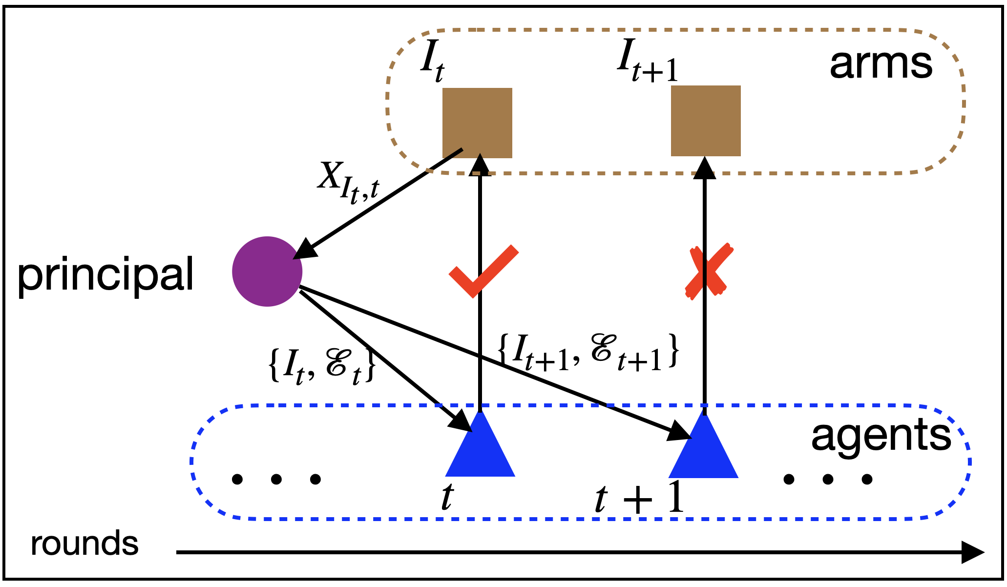
Figure 1: The recommendation process mediated by the principal for two-sided markets.

Consider a two-sided market in which a sequence of $T$ agents arrives sequentially and the principal recommends an arm to each agent. The interaction protocol between agents and principal is as follows. At each round $t\in[T]\equiv\{1,\ldots,T\}$, agent $t$ arrives and observes a message $\mathcal{E}_{t}$ sent by the principal, where $\mathcal{E}_{t}$ is a subset of the information that the principal has collected from all past agents. Next, the principal recommends an arm $I_{t}\in\mathcal{A}\equiv\{1,\ldots,m\}$ to agent $t$. The recommendation is private as each agent observes only the recommendation made to her and does not observe recommendations made to the others. Agent $t$ chooses an action $y_{t}\in\mathcal{Y}\equiv\{0,1\}$, where $y_{t}=1$ if she pulls the recommended arm, and $y_{t}=0$ if she ignores recommendation and does not pull any arm. Finally, agent $t$ leaves the market before round $t+1$. Figure 1 provides an illustration of the process. This model of interaction protocol is equivalent to classical MAB if each agent always pulls the recommended arm. In other words, two models are equivalent if $y_{t}=1$ for any $t\in[T]$. Then a recommendation algorithm would become a bandit algorithm.

2.2 Agent’s Incentive

When an agent $t$ pulls an arm $i\in\mathcal{A}$, the agent receives a stochastic reward $X_{i,t}$ that is drawn i.i.d. from $[0,1]$ with mean $\mu_{i}$. For example, a customer dining in a particular restaurant receives an individual’s subjective observation about this restaurant. This observation could be revealed, for example, by submitting a score or writing a review. Other customers can consume this information through the principal’s recommendations.

We consider that all agents are myopic and choose actions that satisfy an incentive constraint specified as follows. Each agent $t$ has an opportunity cost $c_{t}\in(0,1)$ for pulling an arm, where $c_{t}$ can be the time spent or the price charged. Conditional on $I_{t}$ and $\mathcal{E}_{t}$, we define the agent $t$’s incentive constraint as,

$$\mathbb{E}[X_{I_{t},t}|I_{t}=i,\mathcal{E}_{t}]\geq c_{t},\quad\forall t\in[T],\ \forall i\in\mathcal{A}.$$ (1)

Agent $t$ chooses $y_{t}=1$ if and only if Eq. (1) holds. This incentive model applies to any set $\mathcal{A}$ consisting of multiple arms and generalizes the incentive for two-armed bandits in Che and Hörner (2018). Moreover, Eq. (1) implies that $y_{t}$ is a random variable that depends on information $\mathcal{E}_{t}$ and recommendations $\{I_{1},\ldots,I_{t}\}$.

The incentive constraint in Eq. (1) differs fundamentally from Bayesian Incentive Compatibility (BIC, Kremer et al., 2014; Papanastasiou et al., 2018; Mansour et al., 2020). BIC requires each agent’s Bayesian expected reward to be maximized by the recommended action, conditional on the information flow controlled by the principal, and each agent can evaluate all arms. In contrast, Eq. (1) requires the recommended arm to be at least as good as the opportunity cost. Consequently, Eq. (1) is advantageous in some online marketplaces. First, Eq. (1) applies to a large economy with many arms so that each agent cannot evaluate arms individually. For example, Amazon has numerous similar products, and most customers cannot afford to consider all products due to time constraints. Second, Eq. (1) is useful when the principal only reveals a recommended arm to each agent so that each agent cannot evaluate all arms. For example, Uber only recommends a matched driver to a customer rather than all nearby drivers.

2.3 Information Design for Recommendation

Aggregations and presenting the full observations $\left\{(I_{s},y_{s},X_{I_{s},s}):1\leq s\leq t-1\right\}$ to the future agent $t$ is a crucial value proposition of numerous online marketplaces, such as TripAdvisor, Yelp, and Amazon. The principal faces an information design problem of constructing the message

$$\mathcal{E}_{t}\subseteq\left\{(I_{s},y_{s},X_{I_{s},s}):1\leq s\leq t-1\right\}.$$

The design of $\mathcal{E}_{t}$ needs to consider constraints arising from practical and legal issues that are typically set against information asymmetry.

We are interested in transparent mechanisms for $\mathcal{E}_{t}$, which would disclose the reward history and protect the privacy of recommended arms’ identities. For example, the design of $\mathcal{E}_{t}$ for a particular restaurant would disclose the customers’ historical scores and reviews about this restaurant and protect the identities of specific foods taken by each customer. The explicit forms of $\mathcal{E}_{t}$ depend on whether each agent’s opportunity cost $c_{t}$ in Eq. (1) is known or private to the principal, which will be discussed in a later section.

2.4 Mechanism Design for Recommendation

We also face the mechanism design problem of specifying the available arms for each agent. Different from information design, the mechanism design problem does not control the information structure and is solved by the principal’s recommendation. We focus on a randomized recommendation scheme in which the principal chooses a vector $\mathbf{p}_{t}=(p_{1,t},\ldots,p_{m,t})$ over the set $\mathcal{A}$ and recommends arm $j$ with a probability $p_{j,t}\geq 0$, where $p_{1,t}+\cdots+p_{m,t}=1$ and $t\geq 1$. To implement the randomized recommendation, let $U_{1},U_{2},\ldots$ be independent variables that are uniformly distributed in the interval $[0,1)$. Then the principal’s recommendation $I_{t}$ at round $t$ is chosen by,

$$I_{t}=\sum_{j\in\mathcal{A}}j\cdot\mathbf{1}\left\{U_{t}\in\left[\sum_{s=1}^{j-1}p_{s,t},\sum_{s=1}^{j}p_{s,t}\right)\right\}.$$ (2)

Here the probability vector $\mathbf{p}_{t}$ is determined entirely by agents’ past actions and rewards. That is, $\mathbf{p}_{t}$ does not depend on the past recommendations $I_{1},\ldots,I_{t-1}$. The explicit form of $\mathbf{p}_{t}$ depends on whether the opportunity cost $c_{t}$ in Eq. (1) is known or private to the principal, which will be discussed later in this paper.

There exists another type of recommendation policy called a deterministic policy that is different from Eq. (2). The deterministic policy would fix a pool of future agents a priori and recommend an explore arm to a fraction of agents from the pool (Mansour et al., 2020). Hence, all agents in the pool have the same exploration probability. In contrast, Eq. (2) has an individualized exploration probability in the sense that $p_{j,t}$’s can vary across different agents. Consequently, we will show that a fairness metric can be incorporated into Eq. (2) and thereby improve the recommendation quality.

2.5 Principal’s Objective

The principal receives a signal about the recommended arm $I_{t}$ in the form of agent $t$’s action $y_{t}\in\mathcal{Y}$, and the reward $X_{I_{t},t}$ if $y_{t}=1$. We consider the following loss for the principal,

$$l(I_{t},y_{t})=\max_{i\in\mathcal{A}}\mathbb{E}[X_{i,t}-X_{I_{t},t}\cdot y_{t}],$$ (3)

where the expectation is taken over randomized recommendations and stochastic rewards. Thus, $l(\cdot,\cdot)$ measures the loss for competing against the arm that is optimal in expectation and excludes the random fluctuations in stochastic rewards. Moreover, this loss function depends on the agent’s action $y_{t}$ and can be nonconvex in its first argument $I_{t}$. The principal’s objective is to maximize social welfare. Equivalently, the principal aims to minimize the regret defined by,

$$R_{T}=\sum_{t=1}^{T}l(I_{t},y_{t})-\min_{i\in\mathcal{A}}\sum_{t=1}^{T}l(i,y_{t}).$$ (4)

Then $R_{T}$ measures the realized difference between the cumulative loss and the loss of the optimal arm. Compared to the classical MAB that has a similar objective of minimizing regret, a significant challenge in minimizing regret in Eq. (4) is that action $y_{t}$ is subject to the additional incentive constraint in Eq. (1).

3 Optimal Policy Under Known Opportunity Costs

We start with the scenario where agents’ opportunity costs are known to the principal. To fix ideas, assume the costs are homogeneous, i.e., $c_{t}=c_{*}$ for $t\geq 1$. Then the incentive condition in Eq. (1) is equivalent to

$$\mathbb{E}[X_{I_{t},t}|I_{t}=i,\mathcal{E}_{t}]\geq c_{*},\quad\forall t\in[T]\text{ and }i\in\mathcal{A}.$$

Assume that arm $i=1$’s expected reward is known and greater than the cost,

$$\mu_{1}>c_{*}.$$ (5)

This assumption is without loss of generality because our problem is hopeless if all arms have unknown expected rewards or all expected rewards are less than the cost. In online marketplaces, the initial knowledge of some arm’s expected reward, such as $\mu_{1}$, may arise from product research. For instance, Pandora studied the detailed attributes of music through their music genome project. It may also arise from a flow of customers who may face negligible exploration costs and hence do not mind exploring the arm. Except for arm $i=1$, we allow other arms $i=2,\ldots,m$ to have a priori unknown expected rewards. A fundamental problem for the principal is to design a mechanism for sending the message $\mathcal{E}_{t}$, which will incentivize agents’ exploration of other arms. In this section, we propose a new algorithm that supplies the appropriate incentive and satisfies an important metric on fairness.

3.1 Adaptive Recommendation Policy

We present an algorithm called adaptive recommendation policy (ARP), built upon concepts of “randomized recommendation” and “adaptive exploration.” Specifically, ARP employs the randomized recommendation in Eq. (2), where it selects an arm $i$ according to a probability distribution $\{p_{i,t}:i\in\mathcal{A}\}$ and then recommends it to an arriving agent $t$. Moreover, the probability distribution is adaptive to agents’ historical rewards. If an arm yields inferior rewards, the exploration rate of the subsequent arm will decrease. This adaptivity, in turn, incentivizes the agents’ exploration.

Algorithm 1 Adaptive Recommendation Policy (ARP)

1:Step 1 (Input): Set $\mathcal{A}$; Parameters: $\lambda,\theta_{\tau},k>0$ in Eqs. (6), (7) and (8), respectively.

2:Step 2 (Guarantee incentives): Announce $\mathcal{E}_{t}$ according to Eq. (9). Recommend arm $i=1$ to the first $k$ agents and collect rewards $X_{1,1},\ldots,X_{1,k}$. Let $\hat{\mu}_{1}^{k}=\frac{1}{k}\sum_{s=1}^{k}X_{1,s}$.

3:for each arm $i>1$ in increasing lexicographic order do

4:  Choose $a_{i}^{*}$ and $\mathbf{p}_{t}$ by Eqs. (10) and (11); Update $\mathcal{E}_{t}$ by Eq. (13); Set $\tau_{i}=0$, $L_{i}=0$;

5:  while the counter $\tau_{i}<k$ do

6:    Recommend $I_{t}$ by Eq. (15);

7:      If $I_{t}=i$, update $\tau_{i}=\tau_{i}+1$;

8:    Set $t=t+1$, $L_{i}=L_{i}+1$;

9:  end

10:  Collect $k$ rewards of arm $i$ and calculate the mean reward $\hat{\mu}_{i}^{k}$.

11:end

12:Step 3 (Exploration): Update $\mathcal{E}_{t}$ according to Eq. (16). Initialize $\mathcal{B}=\mathcal{A}$, $q=k$.

13:while the arm set size $|\mathcal{B}|>1$ do

14:  Let $\hat{\mu}_{i}^{q}$ be the mean reward of arm $i$ based on $q$ rewards;

15:  Let $\hat{\mu}^{q}_{*}=\max_{i\in\mathcal{B}}\hat{\mu}_{i}^{q}$, and $\mathcal{B}=\left\{i:\hat{\mu}_{i}^{q}+\sqrt{\frac{\ln(T\theta_{\tau})}{2q}}\geq\max\{\hat{\mu}_{*}^{q},c_{*}\}\right\}$;

16:  For the next $|\mathcal{B}|$ agents, recommend each arm $i\in\mathcal{B}$; Set $q=q+1$.

17:end

18:Step 4 (Exploitation): For the remaining agents, recommend the arm left in $\mathcal{B}$.

We summarize ARP in Algorithm 1, and now detail the main steps. The first step is the input of key parameters. Let $\lambda$ be a margin parameter $\lambda>0$ that satisfies,

$$0<\lambda\leq\frac{3}{4}(\mu_{1}-c_{*}).$$ (6)

Then the upper bound of $\lambda$ depends on the gap between $\mu_{1}$ and $c_{*}$. Let $\tau\in(0,1-c_{*})$, and

$$\theta_{\tau}=\frac{4m^{2}}{\tau\cdot\min_{i\in\mathcal{A}}\mathbb{P}(\mu_{i}-c_{*}\geq\tau)}.$$ (7)

For example, if the prior distribution of $\mu_{i}$ is uniform on $[0,1]$, then $\min_{i\in\mathcal{A}}\mathbb{P}(\mu_{i}-c_{*}\geq\tau)=1-c_{*}-\tau>0$. Given $\theta_{\tau}$, the principal selects a sample size $k>0$ satisfying,

$$k\geq\max\left\{\frac{9}{2\lambda^{2}}\ln\left(\frac{20m}{\lambda}\right),\ \theta_{\tau}^{2}\ln(T\theta_{\tau})\right\},$$ (8)

where $m$ is the number of arms, and $T$ is the time horizon.

The second step is to guarantee the agent’s incentives. We split this step into $m$ stages, where each stage is indexed by $i=1,\ldots,m$. The goal is to collect $k$ samples for each arm $i$. Let $L_{i}$ be the number of rounds at each stage $i$, which is specified later. Consider the initial stage $i=1$. The principal sends the message $\mathcal{E}_{t}$ to agent $t\in\{1,\ldots,k\}$, where

$$\mathcal{E}_{t}=\left\{\mu_{1}>c_{*}\right\}\cup\left\{\text{exploration rate }0\right\}.$$ (9)

Then principal recommends arm $i=1$ to agents $t\in\{1,\ldots,k\}$ according to Eq. (2). Here $\mathbf{p}_{t}$ is given by $p_{1,t}=1$ and $p_{j,t}=0$ for any $j\neq 1$. Conditional on $\mathcal{E}_{t}$ in Eq. (9), each agent $t$ is aware that the recommended arm has a larger expected reward than the opportunity cost. Then the principal collects rewards $X_{1,1},\ldots,X_{1,k}$, and calculates the empirical mean reward $\hat{\mu}_{1}^{k}=\frac{1}{k}\sum_{s=1}^{k}X_{1,s}$ of arm $i=1$. The initial stage has a total of $L_{1}=k$ rounds. Next, we consider stage $i>1$. Here the principal chooses arm $i$ as the explore arm, and it chooses an exploit arm $a_{i}^{*}$ by

$$a_{i}^{*}=\underset{1\leq j\leq i-1}{\arg\max}\leavevmode\nobreak\ \hat{\mu}^{k}_{j},$$ (10)

where ties are broken randomly. The principal specifies the vector $\mathbf{p}_{t}$ in Eq. (2) as,

$$p_{i,t}=\frac{\lambda}{2(c_{*}-\widehat{M}_{i})+\lambda}\mathbf{1}\left\{\widehat{M}_{i}<c_{*}\right\}+\mathbf{1}\left\{\widehat{M}_{i}\geq c_{*}\right\},\quad p_{a_{i}^{*},t}=1-p_{i,t},$$ (11)

and $p_{j,t}=0,\forall j\not\in\{a_{i}^{*},i\}$. Here $\sum_{j=1}^{i-1}L_{j}+1\leq t\leq\sum_{j=1}^{i}L_{j}$, and $\widehat{M}_{i}$ in Eq. (11) is the empirical mean of historical rewards up to the stage $i-1$,

$$\widehat{M}_{i}=\frac{1}{\sum_{j=1}^{i-1}L_{j}}\sum_{s=1}^{L_{1}+\cdots+L_{i-1}}X_{I_{s},s}\cdot y_{s}.$$ (12)

It is seen that the exploration rate $p_{i,t}$ is adaptive to the historical rewards through $\widehat{M}_{i}$. Moreover, the message $\mathcal{E}_{t}$ in stage $i>1$ is updated as follows,

$$\mathcal{E}_{t}=\left\{\mu_{1}>c_{*}\right\}\cup\left\{\text{exploration rate }p_{i,t}\right\}\cup\left\{X_{I_{s},s}:y_{s}=1\text{ and }1\leq s\leq\sum_{j=1}^{i-1}L_{j}\right\}.$$ (13)

Then under $\mathcal{E}_{t}$ in Eq. (13), agent $t$ does not observe past agents’ actions or identities of arms that were recommended to past agents. Indeed, $\mathcal{E}_{t}$ only discloses the information that $\mathcal{A}$ includes a good arm, together with the exploration rate $p_{i,t}$ at the current stage, and the reward history of all agents who have followed the recommendations. Finally, the principal can incorporate each agent’s belief into the recommendation. Suppose that the principal collects historical data and forms a criterion $\mathcal{H}(t)$ where the agent $t$ would like to return even if she receives an unsatisfactory recommendation,

$$\mathcal{H}(t)=\{\text{agent $t$ would like to return to the market if }X_{I_{t},t}<c_{t}\},\ \forall t\in[T],$$ (14)

where in this section $c_{t}=c_{*}$ for $t\geq 1$. We will present an example of $\mathcal{H}(t)$ in Section 3.3. The principal can employ the policy,

$$I_{t}=\sum_{j\in\{a_{i}^{*},i\}}j\cdot\mathbf{1}\left\{U_{t}\in\left[\sum_{s=1}^{j-1}p_{s,t},\sum_{s=1}^{j}p_{s,t}\right)\right\}\cdot\mathbf{1}\{\mathcal{H}(t)\text{ holds}\}+a_{i}^{*}\cdot\mathbf{1}\{\mathcal{H}(t)\text{ fails}\}.$$ (15)

Here $p_{s,t}$ is given by Eq. (11) and $\sum_{j=1}^{i-1}L_{j}+1\leq t\leq\sum_{j=1}^{i}L_{j}$. This policy is a generalization of the randomized recommendation in Eq. (2), by imposing the criterion $\mathcal{H}(t)$. The stage $i$ is concluded after the principal collects a total of $k$ rewards of arm $i$, and the principal can calculate the number of rounds $L_{i}$ and arm $i$’s mean reward $\hat{\mu}_{i}^{k}$ based on $k$ rewards.

The third step is the exploration of arms. After collecting $k$ rewards of each arm in $\mathcal{A}$, the principal updates $\mathcal{E}_{t}$ as follows,

$$\mathcal{E}_{t}=\left\{k\text{ rewards are collected for each arm }i\in\mathcal{A}\right\}.$$ (16)

Next, arms are compared to one another and compete against the cost $c_{*}$. This step is an incentivized version of the Active Arms Elimination algorithm in Even-Dar et al. (2006). Specifically, each arm is initially labeled active and included in a set $\mathcal{B}$. Let $\hat{\mu}_{i}^{q}$ be the empirical mean reward of arm $i$ based on $q$ rewards, where $q\geq k$. Let $\hat{\mu}^{q}_{*}=\max_{i\in\mathcal{B}}\hat{\mu}_{i}^{q}$. Define an arm $i$ to be suboptimal if the following condition holds,

$$\hat{\mu}_{i}^{q}+\sqrt{\frac{\ln(T\theta_{\tau})}{2q}}<\max\left\{\hat{\mu}_{*}^{q},c_{*}\right\}.$$

Here the principal compares each arm with the cost $c_{*}$ and guarantees the agent’s incentive constraint. The suboptimal arms will be permanently eliminated from $\mathcal{B}$. For the next $|\mathcal{B}|$ agents, the principal recommends each arm $i\in\mathcal{B}$ according to an increasing lexicographic order and collects a new reward for each arm $i$. The algorithm repeats the comparison and drops arms over time until only one arm remains.

The fourth step is the exploitation of an arm, where the principal commits to recommending the single arm in $\mathcal{B}$ to the remaining agents.

3.2 Incentive Guarantee

We now study the performance of ARP in Algorithm 1. First, we consider the incentive guarantee. The exploit arm $a_{i}^{*}$ in Eq. (10) is based on empirical mean rewards, whereas the incentive constraint in Eq. (1) is defined based on the expected rewards. Although there exists a discrepancy between the empirical and expected rewards, we show in Theorem 1 that ARP guarantees the agent’s incentive. The key is that we quantify a margin parameter $\lambda>0$ in Eq. (6) to ensure that when the sample size $k$ is large enough to satisfy Eq. (8), there is a high probability that the expected reward of the recommended arm is greater than the opportunity cost. Indeed, if $\lambda=0$, then $k$ needs to be infinitely large to guarantee the agent’s incentive.

Theorem 1

Suppose that the assumption in Eq. (5) holds and parameters $\lambda,\theta_{\tau},k$ are chosen according to Eqs. (6), (7), and (8), respectively. Then ARP in Algorithm 1 guarantees the agent’s incentive in Eq. (1) for any $t\in[T]$ and $i\in\mathcal{A}$.

The ARP has an exploration rate $p_{i,t}$ that is adaptive to historical rewards. Specifically, if $\widehat{M}_{i}<c_{*}$ and the explore arm $i$ yields inferior rewards with $\widehat{M}_{i+1}\leq\widehat{M}_{i}$, then the exploration rate in Eq. (11) for arm $i+1$ would decrease with $p_{i+1,t}\leq p_{i,t}$. If $\widehat{M}_{i}\geq c_{*}$, then the exploration rate in Eq. (11) can take its maximum value as $p_{i,t}=1$. By Theorem 1, this adaptivity is sufficient to guarantee the agent’s incentive. On the other hand, this adaptivity also accelerates exploration. Consider a policy with a fixed exploration rate, then we need to set the rate as $\min_{1<i\leq m}\min_{L_{1}<t\leq T}p_{i,t}$ for each stage $i>1$ in order to guarantee the agent’s incentive. However, this fixed exploration rate may be significantly smaller than most of $p_{i,t}$’s with $i>1$ and $t>L_{1}$, and hence makes the exploration much slower.

3.3 Ex-Post Fairness

We gave a definition of $\mathcal{H}(t)$ in Eq. (14), as the event where agent $t$ would like to return even if she receives an unsatisfactory recommendation. Consider that each agent $t$ has a context $(\alpha_{t},\beta_{t})$. Here $\alpha_{t}$ is the total number of agent $t$’s visits up to (but not including) round $t$. The $\beta_{t}$ is the number of visits up to (but not including) round $t$, where she followed the principal’s recommendation but learned that the received reward was worse than $c_{t}$. Let $\gamma_{t}\in[0,1]$ be the agent $t$’s tolerance level of exploration that is known to the principal. We can now define $\mathcal{H}(t)$ using these parameters as follows,

$$\mathcal{H}(t)=\left\{\frac{\beta_{t}+1}{\alpha_{t}+1}\leq\gamma_{t}\right\},\quad\forall t\geq 1.$$ (17)

We now define a policy as ex-post fair if the policy guarantees that,

$$\frac{\beta_{t}+\mathbf{1}\{\mathbb{E}[X_{I_{t},t}]<c_{t}\}}{\alpha_{t}+1}\leq\gamma_{t},\quad\forall t\geq 1.$$ (18)

Ex-post fairness can be interpreted as protection from over-exploitation of agents, including new and returning agents. For new agents who have data $(\alpha_{t},\beta_{t})=(0,0)$, unless $\gamma_{t}=1$, the principal would recommend exploitation arms to those agents. For returning agents with historical data $(\alpha_{t},\beta_{t})\neq(0,0)$, ex-post fairness guarantees that the unsatisfactory rate is controlled by $\gamma_{t}$. Moreover, $\mathcal{H}(t)$ applies to the setting where agents do not return to the market because we can simply set $\gamma_{t}=1$. A randomized policy such as ARP has personalized exploration rate $p_{i,t}$, which adapts to the agent’s historical data, meets $\mathcal{H}(t)$ for any $t\geq 1$ and satisfies ex-post fairness.

Theorem 2

The ARP procedure in Algorithm 1 satisfies the ex-post fairness criterion in Eq. (18).

We note that there are other fairness criteria in recommendation systems. For example, Kannan et al. (2017) proposed to incentivize fair exploration, in the sense that worse arms will not be preferred to better ones. In contrast, ex-post fairness focuses on the other side of the market, asking that returning agents are never over-exploited.

We also compare ARP with the policy in Mansour et al. (2020), where the latter cannot guarantee ex-post fairness uniformly over all sequences of agents. This is because Mansour et al. employ a deterministic policy. As discussed in Section 2.4, a deterministic policy fixes a pool of agents to explore a given arm, where all agents in the pool have the same probability of being recommended the given arm. Consequently, there may exist a sequence of agents whose historical data fail to lie in $\mathcal{H}(t)$ for some $t$’s. Moreover, we also note that there are three other major differences between ARP and Mansour et al.’s policy. First, the incentive conditions are different. Specifically, ARP and Mansour et al.’s policy are based on the incentive in Eq. (1) and BIC, respectively. Second, the exploration rate in Mansour et al. is not adaptive to historical rewards. Following the discussion of Theorem 1, the nonadaptive policy gives a slower exploration compared to the adaptive policy such as ARP. Finally, Mansour et al.’s policy requires each agent to know the identity of the recommended arm but not the arm’s reward history. In contrast, ARP is transparent in disclosing arms’ reward history and does not reveal arms’ identities.

3.4 Regret Analysis

We provide an upper bound of the regret for ARP. Note that the definition of the regret $R_{T}$ in Eq. (4) depends on the agent’s action $y_{t}$. However, since Theorem 1 respects the agent’s incentive constraint, we show that ARP can achieve the optimal regret bound as if the regret $R_{T}$ does not depend on the agent’s action.

Theorem 3

Suppose the assumption in Eq. (5) holds, and the parameters $\lambda,\theta_{\tau},k$ are chosen by Eqs.  (6), (7), and (8), respectively. Let $\gamma_{t}=1$ in Eq. (17). Then the ARP procedure in Algorithm 1 achieves ex-post regret,

$$R_{T} \leq L^{*}+O\left(\sqrt{mT\ln(mT)}\right),$$

where $L^{*}\equiv L_{1}+\cdots+L_{m}$ is the total number of rounds in Step 2 of ARP, $m$ is the number of arms, and $T$ is the time horizon.

4 Benchmark Recommendation Policies

We now characterize benchmark policies. In the scenario of known opportunity costs, we introduce three benchmarks: full transparency, first-best, and second-best, depending on the information design of $\mathcal{E}_{t}$. The ARP in Algorithm 1 gives an example of the second-best policy. Comparing three benchmark policies helps highlight the role of incentives, in addition to the exploration-exploitation tradeoff in classical MAB.

4.1 Benchmark Policies

We first characterize benchmark policies assuming that each agent’s opportunity cost is known to the principal.

Full Transparency.

The principal truthfully discloses all her information to the agents. Under Assumption 5, all her information is $\mathcal{E}_{t}=\{\mu_{1}>c_{*}\}\cup\left\{(I_{s},y_{s},X_{I_{s},s}):1\leq s\leq t-1\right\}$. Let $a_{t}^{*}=\arg\max_{i\in\mathcal{A}}\{\mu_{1}:i=1\}\cup\{\hat{\mu}_{i,t}:i\neq 1\}$, where

$$\hat{\mu}_{i,t}=\frac{\sum_{s\leq t-1:I_{s}=i}X_{i,s}\cdot y_{s}}{|\{s\leq t-1:I_{s}=i,y_{s}=1\}|},\quad\forall i\neq 1.$$

The full transparency can be implemented using the policy in Eq. (2) with $p_{a_{i}^{*},t}=\mathbf{1}\{\hat{\mu}_{a_{t}^{*},t}\geq c_{*}\}.$ Conditional on the assumption in Eq. (5), full transparency would recommend arm $a_{t}^{*}=1$ to all agents, as the principal has no prior information on other arms. This policy fulfills the principal’s exploitation goal of minimizing the short-term regret of agents.

First-Best Policy.

The principal optimizes her policy $p_{i,t}$ to minimize $R_{T}$ in Eq. (4). By ignoring the incentive constraint in Eq. (1), the first-best policy captures the classical exploration-exploitation tradeoff, as studied in a rich literature of MAB (Rothschild, 1974; Lai and Robbins, 1985; Even-Dar et al., 2006; Bubeck and Cesa-Bianchi, 2012).

Here the first-best policy is implemented in the context of a multi-agent MAB problem. An example of the first-best policy can be implemented by the Active Arms Elimination algorithm proposed by Even-Dar et al. (2006). Note that we provided a version of this algorithm with the incentive guarantee in Section 3.1. Here each arm is initially labeled active and is included in a set $\mathcal{B}$. Let $\hat{\mu}_{i}^{l}$ be the empirical mean reward of arm $i$ based on $l\geq 0$ rewards, where $\hat{\mu}_{i}^{0}=\mu_{1}$ for any $i\in\mathcal{A}$. At each step $l\geq 1$, we set $\hat{\mu}^{l}_{*}=\max_{i\in\mathcal{B}}\hat{\mu}_{i}^{l}$. An arm $i$ is suboptimal if the following condition holds,

$$\hat{\mu}_{i}^{l}+\sqrt{\frac{\ln(T\theta_{\tau})}{2l}}<\hat{\mu}_{*}^{l},$$

where $\theta_{\tau}$ is defined as in Eq. (7). The suboptimal arms are permanently eliminated from $\mathcal{B}$. For the arriving agents, the principal chooses an arm $i\in\mathcal{B}$ in lexicographic order and recommends it to agents until it collects a new reward of arm $i$. This step concludes when the principal collects new rewards of all arms in $\mathcal{B}$, and the algorithm proceeds to step $l+1$. The arms drop out over time until only one arm remains in $\mathcal{B}$, and the principal commits to exploit the single arm in $\mathcal{B}$. It is known that this algorithm enjoys minimax optimality in regret if the incentive constraint in Eq. (1) is ignored (Even-Dar et al., 2006). Comparing first-best and full transparency thus highlights the principal’s exploration goal.

Second-Best Policy.

In this regime, the principal optimizes her policy $p_{i,t}$ to minimize the regret $R_{T}$ subject to the incentive constraint in Eq. (1). The ARP in Algorithm 1 is a second-best policy. Comparing second-best and first-best policies highlights the role of incentives.

4.2 The Role of Incentives

We now discuss ARP as an example of the second-best policy and highlight the role of incentives. Theorem 1 guarantees the agent’s incentive constraint if the exploration rate for arm $i>1$ is no greater than $p_{i,t}$ specified by Eq. (11). That is,

$$p_{i,t}=\frac{\lambda}{2(c_{*}-\widehat{M}_{i})+\lambda}\ \text{ if }\widehat{M}_{i}<c_{*},$$

and $p_{i,t}=1$ if $\widehat{M}_{i}\geq c_{*}$. In words, $p_{i,t}$ is the maximum exploration that the principal can recommend, subject to the incentive constraint. We thus interpret $p_{i,t}$ as the principal’s exploration capacity.

The capacity depends on the historical rewards via $\widehat{M}_{i}$. If $\widehat{M}_{i}\geq c_{*}$, then the agents have myopic incentives to explore, and the principal can employ the full exploration at $p_{i,t}=1$ for arm $i$. Therefore, the incentive constraint in Eq. (1) is never binding in this case.

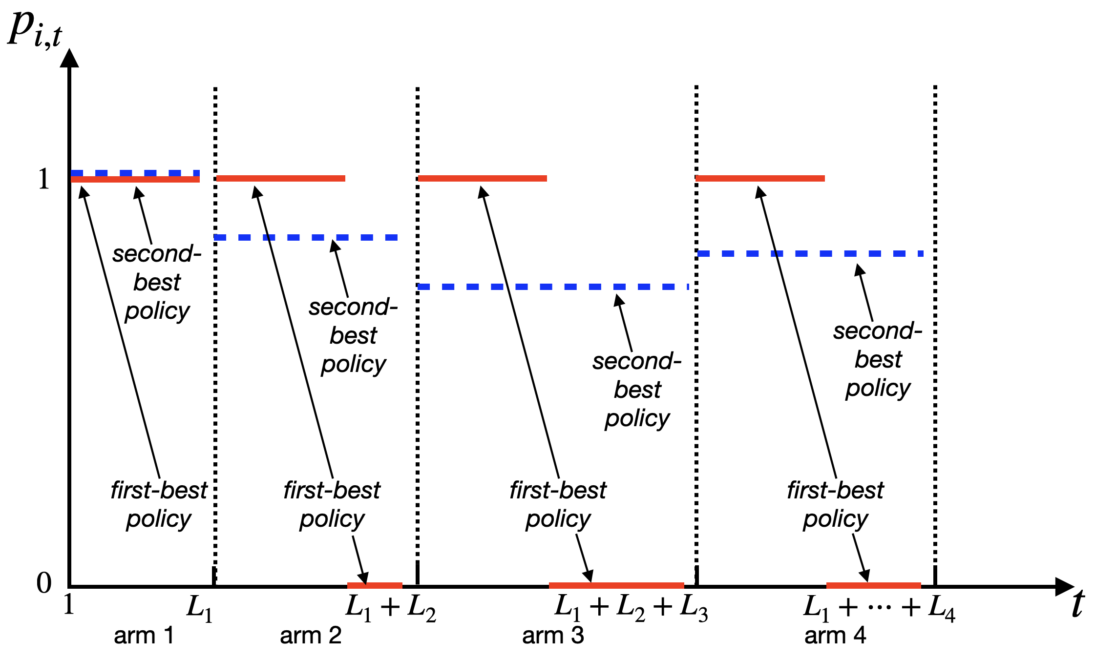
Figure 2: Illustrating paths of $p_{i,t}$ for first-best and second-best policies.

In contrast, if $\widehat{M}_{i}<c_{*}$, the incentive constraint is binding. In this case, the exploration capacity $p_{i,t}<1$, so not all agents are recommended an explore arm. Intuitively, if the principal recommends an explore arm $i$ to all agents at stage $i$ (i.e., $p_{i,t}=1$), the agents will find the recommendation completely uninformative; therefore, their expected reward of the recommended arm equals $\widehat{M}_{i}$. Since $\widehat{M}_{i}<c_{*}$, they will never pull the explore arm $i$. On the other hand, if the principal rarely explores (i.e., $p_{i,t}\approx 0$), then the agent’s expected reward of the recommended arm will be at least $\mu_{1}$; since $\mu_{1}>c_{*}$, the agents will be almost certain that the recommendation is genuine. Naturally, there is an interior level of exploration that will satisfy the incentive constraint. The capacity $p_{i,t}$ is initially one for $i=1$. After exploiting arm $i=1$ with $\mu_{1}>c_{*}$, the principal has built her credibility. As time progresses, the exploration capacity $p_{i,t}$ for each arm $i>1$ will be adaptive to historical rewards.

In essence, the principal pools recommendations across two very different circumstances in ARP: the exploit arm $a_{i}^{*}$, and an explore arm $i$, where $i>1$. Although the agents in the latter case will never knowingly follow the recommendation, pooling the two circumstances for recommendations enables the principal to incentivize the agents to explore, conditional on the designed public information that the recommendation in the latter circumstance is kept sufficiently infrequent. Because the agents do not internalize the benefits of exploration, such pooling becomes a useful tool for the principal’s second-best policy, as implemented in ARP.

Figure 2 depicts the learning trajectories of the first-best and second-best policies, which have a cutoff structure with a maximal feasible exploration. The maximal exploration equals $1$ under the first-best policy in Section 4.1, conditional on the corresponding arm remaining active in set $\mathcal{B}$. Otherwise, no exploration is chosen. The maximal feasible exploration is $p_{i,t}$ under the second-best policy for each arm $i>1$, where $p_{i,t}$ is adaptive to historical rewards. Throughout, $p_{i,t}$ remains $1$ or strictly below $1$. In other words, learning is slower under the second-best policy than that under the first-best policy. The principal needs to experiment longer under the second-best regime than under the first-best regime.

4.3 Cold-Start Problem in Second-Best Policy

Some products (e.g., songs, movies, or books) are relatively unappealing ex ante, so few people will find them worthwhile to explore on their own, even at a zero price. However, exploring these products can be valuable as some are ultimately worth consumption, and the exploration will benefit subsequent users. The lack of sufficient initial discovery is often coined as the cold-start problem, which may lead to the demise of good products (Lika et al., 2014). The challenge lies in that users who explore the products usually do not internalize the benefit accruing to future users. Agents are myopic and choose actions that satisfy the incentive constraint in Eq. (1).

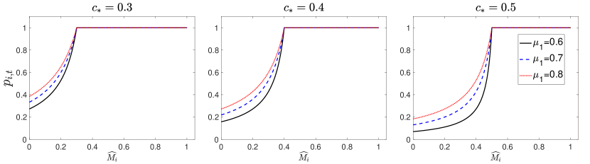
Figure 3: (Second-Best) The exploration rate $p_{i,t}$ in Eq. (11) for arm $i>1$.

The values of $(\mu_{1},c_{*})$ parameterize the severity of the cold-start problem. Figure 3 shows the exploration rate $p_{i,t}$ in Eq. (11) for arm $i>1$. As $\mu_{1}$ decreases or $c_{*}$ increases, it is more difficult for the principal to credibly explore arms, thereby reducing the exploration rate for ARP and making the cold-start problem more severe. On the other hand, when the difference $(\mu_{1}-c^{*})$ increases, the sample size $k$ in Eq. (8) can be smaller for the initial collection of each arm’s rewards. Moreover, the margin parameter $\lambda$ in Eq. (6) can be larger, which leads to an increased exploration rate for ARP and makes the cold-start problem less severe.

Background learning for $\mu_{1}$ seeds the exploration. In particular, the assumption in Eq. (5) would fail if no arm’s expected reward is known or $\mu_{1}<c_{*}$. In either of these cases, the principal has no credibility to induce exploration. This observation has practical implications. For instance, Internet platforms such as Pandora make costly investments to discover $\mu_{1}$, which helps speed up learning and discovery of good products in the second-best regime.

5 Optimal Policy Under Private Opportunity Costs

We now consider that the principal starts with little information about agents’ opportunity costs and directly elicits necessary knowledge of agents’ preferences. Each agent’s opportunity cost can be private and unknown to the principal. In this case, the incentive constraint in Eq. (1) cannot always be satisfied due to the unknown opportunity costs. However, since agents’ actions follow the incentive constraint, their actions can be used as feedback for exploration. This section discusses a second-best policy that satisfies ex-post fairness and achieves minimax regret $R_{T}$ under private opportunity costs.

5.1 Modified Adaptive Recommendation Policy

We propose a modified adaptive recommendation policy (MARP), which is also built upon “randomized recommendation” and “adaptive exploration.” MARP has two new ingredients compared to ARP in Algorithm 1. First, ARP considers only two arms for the recommendation at each round, an explore arm $i$ and an exploit arm $a_{i}^{*}$, and $p_{j,t}=0$ for any $j\in\mathcal{A}\setminus\{a_{i}^{*},i\}$, as specified in Eq. (11). In contrast, MARP considers all arms for the recommendation at each round, where $p_{j,t}\neq 0$ for any $j\in\mathcal{A}$. Second, MARP uses each arm’s cumulative loss as feedback to adjust the probability of recommending each arm, whereas ARP uses the empirical mean of historical rewards as a factor to adjust the probability of recommending each arm.

Algorithm 2 Modified Adaptive Recommendation Policy (MARP)

1:Input: Arm set $\mathcal{A}$; Parameter: $\eta=\sqrt{8(\ln m)/T}$.

2:Initialization: Initialize the cumulative loss $\hat{L}_{i,0}=0,\forall i\in\mathcal{A}$. Announce $\mathcal{E}_{1}$ according to Eq. (19). Choose an arm $i\in\mathcal{A}$ with $p_{i,1}=1/m$ and recommend it to agent $t=1$. Collect a reward if $y_{1}=1$.

3:for each agent $t>1$ in increasing lexicographic order do

4:  For each arm $i\in\mathcal{A}$, compute the estimated loss $\hat{l}(i,y_{t-1})$ in Eq. (21);

5:  Update the estimated cumulative loss $\hat{L}_{i,t-1}=\hat{L}_{i,t-2}+\hat{l}(i,y_{t-1})$;

6:  Update the vector $\mathbf{p}_{t}$ by $p_{i,t}=\frac{\exp(-\eta\cdot\hat{L}_{i,t-1})}{\sum_{i=1}^{m}\exp(-\eta\cdot\hat{L}_{i,t-1})},\forall i\in\mathcal{A}$ in Eq. (22);

7:  Update $\mathcal{E}_{t}$ according to Eq. (23);

8:  Recommend $I_{t}$ in Eq. (24) to agent $t$. Collect a reward for arm $I_{t}$ if $y_{t}=1$.

9:end

We summarize MARP in Algorithm 2 and then detail its main steps. The first step is the input of parameter $\eta>0$. Consider that the time horizon $T$ is known. Let

$$\eta=\sqrt{\frac{8\ln m}{T}},$$

where $m$ is the number of arms. We will extend the algorithm to the case of unknown $T$ later in this section.

The second step is the exploration-exploitation of arms. Since agents’ opportunity costs are heterogeneous and unknown, their actions vis a vis recommendations cannot directly yield an inference of the optimal arm up to a given round. For example, an arm $i\in\mathcal{A}$ whose recommendation is ignored by an agent $j$ does not necessarily have a worse expected reward than another arm $i^{\prime}\in\mathcal{A}$ whose recommendation is followed by another agent $j^{\prime}$, where $i\neq i^{\prime}$ and $j\neq j^{\prime}$. We use a strategy of randomly pooling recommendations across all arms, rather than pooling from only a genuinely good arm and an unknown arm as used in ARP. This approach prevents the optimal arm from being eliminated early. Specifically, for agent $t=1$, the principal sends the following information,

$$\mathcal{E}_{1} =\left\{p_{i,1}=\frac{1}{m},\ \forall i\in\mathcal{A}\right\}.$$ (19)

Then the principal recommends arm $I_{1}$ to agent $t=1$ according to the policy in Eq. (2), where the vector $\mathbf{p}_{t}$ is given by $p_{i,1}=1/m$ for any $i\in\mathcal{A}$. Conditional on $\mathcal{E}_{1}$ in Eq. (19), agent $t=1$ is aware of the randomized policy. The principal collects a reward $X_{I_{1},1}$ if $y_{1}=1$, that is, if agent $t=1$ pulls the recommended arm $I_{1}$.

Next, we consider agent $t>1$. Here the principal considers all arms for the recommendation, where the $\mathbf{p}_{t}$ in Eq. (2) is specified as,

$$p_{i,t}=\frac{\exp\left(-\eta\cdot\sum_{s=1}^{t-1}l(i,y_{s})\right)}{\sum_{j=1}^{m}\exp\left(-\eta\cdot\sum_{s=1}^{t-1}l(j,y_{s})\right)},\quad\text{for }i\in\mathcal{A}.$$ (20)

The $\eta$ is a parameter with $\eta>0$, and $l(i,y_{s})$ is the loss function defined in Eq. (3). It is seen that MARP uses the agent’s action $y_{s}$ and loss $l(i,y_{s})$ as feedback to update $p_{i,t}$. Moreover, $p_{i,t}$ in Eq. (20) is adaptive to the historical data through the cumulative loss $\sum_{s=1}^{t-1}l(i,y_{s})$ for each $i\in\mathcal{A}$. This is intuitive because $p_{i,t}$ should be large for an arm $i$ with a small cumulative loss. In contrast, ARP in Algorithm 1 is adaptive to the historical rewards through the empirical mean of the historical rewards $\widehat{M}_{i}$ in Eq. (11). Note that $\widehat{M}_{i}$ does not differentiate each arm’s individual rewards. Thus, the adaptivity of MARP is different from that of ARP. An explanation of this difference is that if the opportunity costs are known, ARP can infer an optimal arm conditional on the information up to a given round and then uses this arm as an exploit arm. From the agent’s perspective, they can infer the quality of this exploit arm through the empirical mean of historical rewards, which directly determines the largest exploration rate in ARP. However, given private opportunity costs, an agent’s action $y_{s}$ towards an arm $i\in\mathcal{A}$ provides little insight into the other agents’ actions $y_{s^{\prime}}$ towards the same arm $i\in\mathcal{A}$. As a solution, MARP traces down the individual loss of each arm $i\in\mathcal{A}$ and gradually improves recommendations by adjusting $p_{i,t}$ over time.

We consider a practical approach to compute $p_{i,t}$ in Eq. (20). Note that $p_{i,t}$ remains unchanged if we let $l(i,y_{s})=\mathbb{E}[-X_{I_{s},s}\cdot y_{s}]$, where the expectation is taken over randomized $I_{t}$ and stochastic reward $X_{I_{t},t}$. An estimator for $l(i,y_{s})$ is given by,

$$\hat{l}(i,y_{s})=\begin{cases}-X_{i,s}\cdot y_{s}/p_{i,s},&\text{ if }I_{s}=i,\\ 0,&\text{ if }I_{s}\neq i,\end{cases}\quad\forall i\in\mathcal{A}\text{ and }1\leq s\leq t-1,$$ (21)

where $X_{i,s}$ is the collected reward if $y_{s}=1$. Then $\hat{l}(i,y_{s})$ is unbiased since $\mathbb{E}\left[\hat{l}(i,y_{s})\right]=\sum_{j=1}^{m}p_{j,s}\mathbb{E}\left[-X_{i,s}\cdot y_{s}/p_{i,s}\right]\mathbf{1}_{j=i}=\mathbb{E}\left[-X_{I_{s},s}\cdot y_{s}\right]$. Hence we can update $p_{i,t}$ in Eq. (20) using the estimator $\hat{l}(i,y_{s})$,

$$p_{i,t}=\frac{\exp\left(-\eta\cdot\sum_{s=1}^{t-1}\hat{l}(i,y_{s})\right)}{\sum_{j=1}^{m}\exp\left(-\eta\cdot\sum_{s=1}^{t-1}\hat{l}(j,y_{s})\right)},\quad\text{for }i\in\mathcal{A}.$$ (22)

Next, the message $\mathcal{E}_{t}$ for agent $t>1$ is updated as,

$$\mathcal{E}_{t}= \left\{p_{i,t}\propto\text{the exponential of arm $i$'s cumulative reward,}\ \forall i\in\mathcal{A}\right\}$$ (23)

$$\cup\left\{X_{I_{s},s}:y_{s}=1\text{ and }1\leq s\leq t-1\right\}.$$

Under $\mathcal{E}_{t}$ in Eq. (23), agents do not observe past agents’ actions or the identities of the arms that were recommended to past agents. Instead, $\mathcal{E}_{t}$ is transparent in disclosing the history of rewards received by past agents who have followed the recommendations.

The principal can incorporate each agent’s belief $\mathcal{H}(t)$ into the recommendation. In particular, the principal can employ the following policy,

$$I_{t}= \leavevmode\nobreak\ \sum_{j\in\mathcal{A}}j\cdot\mathbf{1}\left\{U_{t}\in\left[\sum_{s=1}^{j-1}p_{s,t},\sum_{s=1}^{j}p_{s,t}\right)\right\}\cdot\mathbf{1}\{\mathcal{H}(t)\text{ holds}\}$$ (24)

$$\quad\quad+\left[\underset{j\in\mathcal{A}}{\arg\min}\sum_{s=1}^{t-1}\hat{l}(j,y_{s})\right]\cdot\mathbf{1}\{\mathcal{H}(t)\text{ fails}\}.$$

Here $\hat{l}(i,y_{s})$ and $p_{s,t}$ are given by Eq. (21) and Eq. (22), respectively. This policy is a generalization of the randomized recommendation in Eq. (2), with an additional criterion $\mathcal{H}(t)$. After recommending an arm to agent $t$, the principal collects a reward $X_{I_{t},t}$ if $y_{t}=1$.

5.2 Performance Analysis for MARP

We provide the performance analysis for MARP in Algorithm 2. First, we show that although now agents’ opportunity costs are unknown, MARP satisfies ex-post fairness defined in Eq. (18).

Theorem 4

The MARP procedure in Algorithm 2 satisfies the ex-post fairness criterion in Eq. (18).

Next, we provide the regret analysis for the MARP procedure. The following theorem establishes a nonasymptotic regret bound.

Theorem 5

If the parameters $\eta=\sqrt{(8\ln m)/T}$ and $\gamma_{t}\equiv 1$ in Eq. (17), then for any arm set $\mathcal{A}$ and action sequence $\{y_{t}\}_{t=1}^{T}\in\mathcal{Y}^{T}$, the MARP procedure in Algorithm 2 satisfies, with probability at least $1-\delta$ for any $\delta\in(0,1)$,

$$R_{T}\leq\sqrt{\frac{T}{2}\ln m}+\sqrt{\frac{T}{2}\ln\frac{1}{\delta}},$$

where $R_{T}$ is defined in Eq. (4), $T$ is the time horizon, and $m$ is the number of arms.

To minimize the regret in Eq. (4), it is clear that any deterministic policy of the principal is insufficient. This is because there exists an action sequence $\{y_{t}\}_{t=1}^{T}$ such that the principal has the loss, $l(I_{t},y_{t})=1$, at every time instant $t$. However, the randomization in Eq. (24) guarantees the sublinear regret bound in terms of $T$ even when the loss function $l(\cdot,\cdot)$ in Eq. (3) is nonconvex, as shown in Theorem 5. Moreover, using the classical notion of Hannan consistency in games (Hannan, 1957), it is clear that MARP is Hannan consistent as $\lim\sup_{T\to\infty}R_{T}/T=0$.

Next, we establish a corresponding lower bound for regret. Define the minimax regret for this problem as

$$R^{\dagger}_{T}\equiv\inf_{\{I_{t}\}_{t=1}^{T}}\sup_{\{\mathcal{A}:|\mathcal{A}|=m\},\{y_{t}\}_{t=1}^{T}\in\mathcal{Y}^{T}}R_{T},$$

where the infimum is taken over all possible recommendation policies $\{I_{t}\}_{t=1}^{T}$, and the supremum is taken over all possible classes of $m$ arms and sequences of $T$ actions. Then $R^{\dagger}_{T}$ measures the best possible performance of a recommendation policy.

Theorem 6

For any arm set $\mathcal{A}$ and action sequence $\{y_{t}\}_{t=1}^{T}\in\mathcal{Y}^{T}$, the minimax regret $R^{\dagger}_{T}$ satisfies

$$\lim_{m\to\infty}\lim_{T\to\infty}\frac{R^{\dagger}_{T}}{(1-\epsilon_{T})\sqrt{T\ln m/2}}=1,$$

where $\epsilon_{T}>0$ is any parameter with $\lim_{T\to\infty}\epsilon_{T}=0$.

This theorem implies that the upper regret bound by MARP in Theorem 5 is essentially unimprovable. On the other hand, ARP also achieves a comparable bound of $O(\sqrt{T})$ in Theorem 3. Although the two algorithms achieve similar levels of regret, there exists a key difference between them due to the tradeoff of knowing additional information about opportunity costs and the incentive guarantee. First, ARP requires knowledge of the opportunity costs, which is unnecessary for implementing MARP. Second, ARP guarantees the agent’s incentive as shown in Theorem 1, while MARP does not enjoy such a guarantee.

5.3 Unknown Round Information

The MARP algorithm has the disadvantage that it requires knowledge of the time horizon $T$ in advance. Hence the result in Theorem 5 does not hold uniformly over sequences of agents with any length but only for sequences of agents with a given length $T$. However, we show that if MARP in Algorithm 2 is equipped with a time-varying parameter $\eta=\sqrt{8(\ln m)/t}$, then it yields a near-optimal regret bound for any unknown $T$. The following theorem applies to the nonconvex loss $l$ and the estimated loss $\hat{l}$ in Algorithm 2.

Theorem 7

If the parameter $\eta$ is chosen as $\eta_{t}=\sqrt{(8\ln m)/t}$ for $t\geq 1$, then for any arm set $\mathcal{A}$ and action sequence $\{y_{t}\}_{t=1}^{T}\in\mathcal{Y}^{T}$, the MARP procedure in Algorithm 2 satisfies, with probability at least $1-\delta$ for any $\delta\in(0,1)$,

$$R_{T}\leq\sqrt{2T\ln m}+\sqrt{\frac{\ln m}{8}}+\sqrt{\frac{T}{2}\ln\frac{1}{\delta}},$$

where $R_{T}$ is defined in Eq. (4), $T$ is the time horizon, and $m$ is the number of arms.

6 Related Work

We review related work from multiple kinds of literature, including mechanism design, matching markets, social learning, and Bayesian persuasion.

Mechanism Design

There is a growing body of literature on the intersection of mechanism design and incentivized exploration. When the incentives are created via information asymmetry rather than via monetary transfers, Kremer et al. (2014) derived the Bayesian-optimal policy for a two-arm model. Papanastasiou et al. (2018) considered a similar model but with time-discounted rewards. Bahar et al. (2015) extended the setting in Kremer et al. (2014) to a known social network on the agents, where agents observe friends’ recommendations but not their rewards. Che and Hörner (2018) considers a continuum of agents for a model of two arms and binary rewards. Mansour et al. (2020) extended the BIC policy to a model of multiple arms, a setting which is similar to ours except that we adopt different incentive constraints and allow agents to return. A closely related line of work considers the “full revelation” scenario (see, e.g., Bastani et al., 2021; Kannan et al., 2018; Schmit and Riquelme, 2018), where each agent sees the full history and chooses an action based on her own incentives. This corresponds to the full transparency in Section 4.1 and is different from our policy that satisfies the second-best regime.

Matching Markets

The current paper focuses on two-sided markets without monetary payments, which is related to matching markets (Gale and Shapley, 1962; Shapley and Shubik, 1971; Roth and Sotomayor, 1990). Many two-sided matching markets function through centralized clearinghouses: medical residents to hospitals, children to high schools, commissioned officers to military posts, and college students to dorms. In principle, centralized clearinghouses act as principals that have the advantage of enforcing agents’ decisions and implementing desirable outcomes such as stable matchings. In contrast, our model has a principal that cannot enforce agents’ decisions and is thereby different from centralized matching markets. There are other matching markets organized in a decentralized manner such that each agent makes their decision independently of others’ decisions (Roth and Xing, 1997; Dai and Jordan, 2021a, b). Examples include college admissions, decentralized labor markets, and online dating. In contrast, the model proposed in this paper allows the principal to coordinate the market through recommendations. Hence it is different from existing models of decentralized matching markets.

Social Learning

The field of social learning studies self-interested agents that jointly learn over time in a shared environment (Bikhchandani et al., 1992; Banerjee, 1992; Smith and Sørensen, 2000). Here the agents take actions myopically, ignoring their effects on the learning and welfare of agents in the future. In particular, Bolton and Harris (1999) analyzed a continuous-time game of strategic experimentation in multi-agent two-armed bandits, which consists of a safe arm that offers a known payoff and a risky arm of an unknown type. Keller et al. (2005) studied a similar model but with the feature that the risky arm might yield payoffs after exponentially distributed random times. If the risky arm is good, it generates positive payoffs after exponentially distributed random times; if it is bad, it never pays out anything. Klein and Rady (2011) and Halac et al. (2016) further generalized the strategic experimentation framework to more realistic settings. These models are different from ours as they have no coordination, such as the principal’s recommendations.

Bayesian Persuasion

The models on Bayesian persuasion consider how a principal can credibly manipulate a single agent’s belief and influence her behavior (Aumann et al., 1995; Ostrovsky and Schwarz, 2010; Rayo and Segal, 2010; Kamenica and Gentzkow, 2011). This is an idealized model for many real-life scenarios in which a more informed principal wishes to persuade the agent to take an action that benefits the principal. A single round of our model coincides with a version of the Bayesian persuasion game. Recently, Bergemann and Morris (2016) studied information design for messages that the agents receive in a game. There is also burgeoning literature that studies Bayesian persuasion in dynamic settings (Ely et al., 2015; Halac et al., 2016; Ely, 2017). In these models, the principal has more information than a single agent due to the feedback from the previous agents. Our model also employs such information asymmetry to ensure the desired incentives. The differences are that we consider a multi-agent setting and use the recommendation as a mechanism.

7 Discussion

The design of recommender systems that respect incentives is a crucial need in order for users to be able to discover and choose valued products on a large scale. We have shown how information design and randomized recommendation can promote exploration, regardless of whether the agents’ opportunity costs are known. A key aspect of an agent’s incentive to explore is her belief about an arm. Our proposed recommendation policy allows the principal to pool recommendations across genuinely good arms and unknown arms. Although the agents in the latter case will never knowingly follow the recommendation, pooling the two circumstances for recommendations enables the principal to incentivize the agents to explore. We have also highlighted several factors that could improve exploration in online marketplaces, such as randomization, adaptivity, and background learning.

It is possible to extend the incentive-aware recommender system paradigm to other applications. For example, contextual bandits are important problems in machine learning, where each agent is characterized by a signal, called the context, observable by both the agent and the principal before the principal makes the recommendation. The context can include demographics, tastes, and other agent-specific information, and it impacts the expected rewards received by this agent. Contextual bandits are practically important: for instance, websites that make recommendations may possess a large amount of information about their customers and would like to use this context to adjust their recommendations (e.g., Amazon and Netflix). Another intriguing question is to apply incentive-aware recommender systems to the adaptive clinical trial (ACT) designs for medical drugs. The ACT modifies the course of the trial based on the accumulating results of the trial, typically by adjusting the doses of medicine and adding or removing patients from the trial (Detry et al., 2012). Here an important aspect is the incentives for the patients and doctors to participate in and stay on the trial. It is crucial to manage their beliefs, which can be affected when the prescribed treatment changes throughout the trial. We leave these questions for future research.

Appendix A Technical Proofs

A.1 Proof of Theorem 1

Proof  ARP has two main steps: (i) the sampling step, which collects $k$ rewards from each arm, and (ii) the exploration-exploitation step, where the agents explore the arms based on the collected sample and then identify an exploit arm. We now discuss the incentive constraints for the two steps separately.

The sampling step

This phase can be divided into $m$ stages, where each stage, $i=1,\ldots,m$, lasts $L_{i}$ rounds and $L_{1}=1$. We will show that each agent $t$ in each stage $i$ is incentivized to pull the recommended arm. For an agent $t$ in the stage $i$, the incentive constraint in Eq. (1) is equivalent to

$$\mathbb{E}[X_{I_{t},t}-c_{*}|I_{t}=i,\mathcal{E}_{t}]\cdot\mathbb{P}(I_{t}=i)\geq 0.$$ (25)

Agent $t$ is in the “explore group” with probability $p_{i,t}$ and in the “exploit group” with probability $1-p_{i,t}$. Conditional on being in the explore group and seeing the public information $\mathcal{E}_{t}$ in Eq. (13), the expected gain from following the recommendation $I_{t}$ is $\widehat{M}_{i}$. Here $\widehat{M}_{i}$ is the empirical mean of historical rewards up to stage $i-1$,

$$\widehat{M}_{i}=\frac{1}{\sum_{j=1}^{i-1}L_{j}}\sum_{s=1}^{L_{1}+\cdots+L_{i-1}}X_{I_{s},s}y_{s}.$$

On the other hand, conditional on being in the exploit group and conditional on $\mathcal{E}_{t}$, the expected gain from following the recommendation $I_{t}$ can be analyzed as follows. Define the event $\mathcal{C}_{1}$ as,

$$\mathcal{C}_{1}=\left\{\hat{\mu}_{a_{i}^{*}}^{k}-\lambda\geq c_{*}\right\}.$$

Then the expected gain from following the recommendation $I_{t}$ is at least

$$\mathbb{E}[X_{I_{t},t}|I_{t}=a_{i}^{*},\mathcal{E}_{t},\mathcal{C}_{1}]\cdot\mathbb{P}(\mathcal{C}_{1}).$$

Combining the above two scenarios, we have

$$\mathbb{E}[X_{I_{t},t}-c_{*}|I_{t}=i,\mathcal{E}_{t}]\cdot\mathbb{P}(I_{t}=i)$$

$$\geq\left(\widehat{M}_{i}-c_{*}\right)p_{i,t}+\mathbb{E}[X_{I_{t},t}-c_{*}|I_{t}=a_{i}^{*},\mathcal{E}_{t},\mathcal{C}_{1}]\mathbb{P}(\mathcal{C}_{1})\left(1-p_{i,t}\right).$$

Thus, it suffices to choose $p_{i,t}$ as follows to guarantee the constraint in Eq. (25),

$$p_{i,t}\leq\frac{\mathbb{E}[X_{I_{t},t}-c_{*}|I_{t}=a_{i}^{*},\mathcal{E}_{t},\mathcal{C}_{1}]\mathbb{P}(\mathcal{C}_{1})}{\mathbb{E}[X_{I_{t},t}-c_{*}|I_{t}=a_{i}^{*},\mathcal{E}_{t},\mathcal{C}_{1}]\mathbb{P}(\mathcal{C}_{1})+c_{*}-\widehat{M}_{i}}.$$

Define the parameter $\epsilon\equiv\lambda\sigma_{i}/3$. Recall that $\hat{\mu}^{k}_{i}$ is the empirical mean reward of arm $i$. Consider the event

$$\mathcal{C}_{2}=\{\forall i\in\mathcal{A}:|\hat{\mu}^{k}_{i}-\mu_{i}|\leq\epsilon\}.$$

Using the Chernoff-Hoeffding bound and the union bound,

$$\forall\mu_{1},\ldots,\mu_{m}:\ \mathbb{P}(\mathcal{C}_{2})\geq 1-2m\cdot e^{-2\epsilon^{2}k}.$$

From Eq. (5), $\mu_{1}>c_{*}$. We let $0<\lambda\leq 3(\mu_{1}-c_{*})/4$. Then under the event $\mathcal{C}_{2}$,

$$\hat{\mu}_{1}^{k}-\lambda\sigma_{1} =(\hat{\mu}_{1}^{k}-\mu_{1})+(\mu_{1}-\lambda\sigma_{1})$$

$$\geq-\epsilon+(\epsilon+c_{*})=c_{*}.$$

By definition, $\hat{\mu}_{a_{i}^{*}}^{k}-\lambda\geq\hat{\mu}_{1}^{k}-\lambda$. Hence we have

$$\mathbb{P}(\mathcal{C}_{1}|\mathcal{C}_{2})=1\text{ and }\mathbb{P}(\mathcal{C}_{1},\mathcal{C}_{2})=\mathbb{P}(\mathcal{C}_{2})\mathbb{P}(\mathcal{C}_{1}|\mathcal{C}_{2})=\mathbb{P}(\mathcal{C}_{2}),$$

which implies that

$$\mathbb{E}[X_{I_{t},t}-c_{*}|I_{t}=a_{i}^{*},\mathcal{E}_{t},\mathcal{C}_{1}]\mathbb{P}(\mathcal{C}_{1})$$

$$=\mathbb{E}[X_{I_{t},t}-c_{*}|I_{t}=a_{i}^{*},\mathcal{E}_{t},\mathcal{C}_{1},\mathcal{C}_{2}]\mathbb{P}(\mathcal{C}_{1},\mathcal{C}_{2})+\mathbb{E}[X_{I_{t},t}-c_{*}|I_{t}=a_{i}^{*},\mathcal{E}_{t},\mathcal{C}_{1},\neg\mathcal{C}_{2}]\mathbb{P}(\neg\mathcal{C}_{2})$$

$$\geq\mathbb{E}[X_{I_{t},t}-c_{*}|I_{t}=a_{i}^{*},\mathcal{E}_{t},\mathcal{C}_{1},\mathcal{C}_{2}]\mathbb{P}(\mathcal{C}_{2})-2m\cdot e^{-2\epsilon^{2}k}.$$

Observe that,

$$\mathbb{E}[X_{I_{t},t}-c_{*}|I_{t}=a_{i}^{*},\mathcal{E}_{t},\mathcal{C}_{1},\mathcal{C}_{2}]$$

$$=\mathbb{E}[X_{I_{t},t}-\hat{\mu}_{i}^{k}|I_{t}=a_{i}^{*},\mathcal{E}_{t},\mathcal{C}_{1},\mathcal{C}_{2}]+\mathbb{E}[\hat{\mu}_{i}^{k}-c_{*}|I_{t}=a_{i}^{*},\mathcal{E}_{t},\mathcal{C}_{1},\mathcal{C}_{2}]$$

$$\geq-\epsilon+\lambda.$$

Thus,

$$\mathbb{E}[X_{I_{t},t}-c_{*}|I_{t}=a_{i}^{*},\mathcal{E}_{t},\mathcal{C}_{1}]\mathbb{P}(\mathcal{C}_{1})$$

$$\geq(\lambda-\epsilon)\mathbb{P}(\mathcal{C}_{2})-2m\cdot e^{-2\epsilon^{2}k}$$

$$\geq(\lambda-\epsilon)\left(1-2m\cdot e^{-2\epsilon^{2}k}\right)-2m\cdot e^{-2\epsilon^{2}k}.$$

We let

$$k\geq\frac{9}{2\lambda^{2}}\ln\left(\frac{20m}{\lambda}\right).$$

Then,

$$\mathbb{E}[X_{I_{t},t}-c_{*}|I_{t}=a_{i}^{*},\mathcal{E}_{t},\mathcal{C}_{1}]\mathbb{P}(\mathcal{C}_{1})\geq\frac{3}{5}\lambda-\frac{1}{10}\lambda=\frac{1}{2}\lambda.$$

Thus, it suffices to choose

$$p_{i,t}\leq\frac{\lambda}{2(c_{*}-\widehat{M}_{i})+\lambda}.$$

Since $0\leq p_{i,t}\leq 1$, it suffices to choose

$$p_{i,t}=\frac{\lambda}{2(c_{*}-\widehat{M}_{i})+\lambda}\mathbf{1}\{0\leq\widehat{M}_{i}<c_{*}\}+\mathbf{1}\{\widehat{M}_{i}\geq c_{*}\}.$$

The exploration-exploitation step

We will show that any agent $t$ in this phase satisfies the incentive constraint in Eq. (25),

$$\mathbb{E}[X_{I_{t},t}-c_{*}|I_{t}=i,\mathcal{E}_{t}]\cdot\mathbb{P}(I_{t}=i)\geq 0.$$

Let $l_{*}=\theta_{\tau}^{2}\ln(T\theta_{\tau})$. By Eq. (8), $k\geq l_{*}$. Let $\gamma_{l}=\sqrt{\frac{\ln(T\theta_{\tau})}{2l}}$ for any $l\geq k$. We have that

$$\gamma_{l} \leq\gamma_{l_{*}}=\sqrt{\frac{\ln(T\theta_{\tau})}{2l_{*}}}=\sqrt{\frac{\ln(T\theta_{\tau})}{2\theta_{\tau}^{2}\ln(T\theta_{\tau})}}=\frac{\tau\cdot\min_{i\in\mathcal{A}}\mathbb{P}(\mu_{i}-c_{*}\geq\tau)}{4\sqrt{2}m^{2}}$$ (26)

$$<\frac{\tau}{4}\min_{i\in\mathcal{A}}\mathbb{P}(\mu_{i}-c_{*}\geq\tau),\quad\forall l\geq k.$$

Define the following event,

$$\mathcal{C}_{3}=\left\{\forall l\geq k,\forall i\in\mathcal{A}:|\hat{\mu}_{i}^{l}-\mu_{i}|<\gamma_{l}\right\}.$$

By the Chernoff-Hoeffding bound and the union bound, we have

$$\mathbb{P}(\neg\mathcal{C}_{3}) \leq\sum_{l\geq k}\sum_{i\in\mathcal{A}}\mathbb{P}(|\hat{\mu}_{i}^{l}-\mu_{i}|\geq\gamma_{l})\leq\sum_{l\geq k}\sum_{i\in\mathcal{A}}e^{-2l\cdot\gamma_{l}^{2}}$$

$$\leq T\cdot m\cdot e^{-\ln(T\theta_{\tau})}\leq\frac{m}{\theta_{\tau}}.$$

Now we analyze the incentive condition. Since $X_{I_{t},t}\in[0,1]$ and $c_{*}\in(0,1)$, we have

$$\mathbb{E}[X_{I_{t},t}-c_{*}|I_{t}=i,\mathcal{E}_{t}]\cdot\mathbb{P}(I_{t}=i)$$ (27)

$$=\mathbb{E}[X_{I_{t},t}-c_{*}|I_{t}=i,\mathcal{E}_{t},\mathcal{C}_{3}]\cdot\mathbb{P}(I_{t}=i,\mathcal{C}_{3})$$

$$\quad\quad+\mathbb{E}[X_{I_{t},t}-c_{*}|I_{t}=i,\mathcal{E}_{t},\neg\mathcal{C}_{3}]\cdot\mathbb{P}(I_{t}=i,\neg\mathcal{C}_{3})$$

$$\geq\mathbb{E}[X_{I_{t},t}-c_{*}|I_{t}=i,\mathcal{E}_{t},\mathcal{C}_{3}]\cdot\mathbb{P}(I_{t}=i,\mathcal{C}_{3})-\frac{m}{\theta_{\tau}}.$$

We shall focus on the integral $\mathbb{E}[X_{I_{t},t}-c_{*}|I_{t}=i,\mathcal{E}_{t},\mathcal{C}_{3}]$. If $\mathbb{E}[X_{I_{t},t}-c_{*}|I_{t}=i,\mathcal{E}_{t},\mathcal{C}_{3}]\leq-2\gamma_{l}$, then because

$$\hat{\mu}_{i}^{l}-c_{*}<\mu_{i}-c_{*}+\gamma_{l}\leq-\gamma_{l},$$

we must have already eliminated this arm $i$. Thus, in that case, $I_{t}=i$ cannot occur. If $\mathbb{E}[X_{I_{t},t}-c_{*}|I_{t}=i,\mathcal{E}_{t},\mathcal{C}_{3}]\geq-2\gamma_{l}$ and have the following lower bound,

$$\mathbb{E}[X_{I_{t},t}-c_{*}|I_{t}=i,\mathcal{E}_{t},\mathcal{C}_{3}]\cdot\mathbb{P}(I_{t}=i,\mathcal{C}_{3})$$

$$\geq\tau\cdot\mathbb{P}(\mathcal{C}_{3},\mu_{i}-c_{*}\geq\tau)+0\cdot\mathbb{P}(\mathcal{C}_{3},0\leq\mu_{i}-c_{*}\leq\tau)$$

$$\quad\quad-2\gamma_{l}\cdot\mathbb{P}(\mathcal{C}_{3},-2\gamma_{l}\leq\mu_{i}-c_{*}\leq 0)$$

$$\geq\tau\cdot\mathbb{P}(\mathcal{C}_{3},\mu_{i}-c_{*}\geq\tau)-2\gamma_{l}$$

$$>\tau\cdot\mathbb{P}(\mathcal{C}_{3},\mu_{i}-c_{*}\geq\tau)-\frac{\tau\cdot\mathbb{P}(\mu_{i}-c_{*}\geq\tau)}{2},$$

where the last step is by Eq. (26). Moreover, we can lower bound $\mathbb{P}(\mathcal{C}_{3},\mu_{i}-c_{*}\geq\tau)$ using the Chernoff-Hoeffding bound,

$$\mathbb{P}(\mathcal{C}_{3},\mu_{i}-c_{*}\geq\tau) =\mathbb{P}(\mathcal{C}_{3}|\mu_{i}-c_{*}\geq\tau)\cdot\mathbb{P}(\mu_{i}-c_{*}\geq\tau)$$

$$\geq\left(1-\sum_{l\geq k}\sum_{i\in\mathcal{A}}e^{-2l\cdot\gamma_{l}^{2}}\right)\cdot\mathbb{P}(\mu_{i}-c_{*}\geq\tau)$$

$$\geq\left(1-\frac{m}{\theta_{\tau}}\right)\cdot\mathbb{P}(\mu_{i}-c_{*}\geq\tau)$$

$$>\frac{3}{4}\mathbb{P}(\mu_{i}-c_{*}\geq\tau),$$

where last step above is due to $\theta_{\tau}=4m^{2}/[\tau\min_{i\in\mathcal{A}}\mathbb{P}(\mu_{i}-c_{*}\geq\tau)]$, and

$$\frac{m}{\theta_{\tau}}=\frac{m}{4m^{2}}\cdot\tau\cdot\min_{i\in\mathcal{A}}\mathbb{P}(\mu_{i}-c_{*}\geq\tau)<\frac{1}{4}.$$ (28)

Thus, we have

$$\mathbb{E}[X_{I_{t},t}-c_{*}|I_{t}=i,\mathcal{C}_{3}]\cdot\mathbb{P}(I_{t}=i,\mathcal{E}_{t},\mathcal{C}_{3})>\frac{\tau}{4}\cdot\mathbb{P}(\mu_{i}-c_{*}\geq\tau).$$

Plugging this back to Eq. (27) and using the fact that $\theta\geq\theta_{\tau}$, we obtain that

$$\mathbb{E}[X_{I_{t},t}-c_{*}|I_{t}=i,\mathcal{E}_{t}]\cdot\mathbb{P}(I_{t}=i)$$

$$\geq\mathbb{E}[X_{I_{t},t}-c_{*}|I_{t}=i,\mathcal{E}_{t},\mathcal{C}_{3}]\mathbb{P}(I_{t}=i,\mathcal{C}_{3})-\frac{m}{\theta_{\tau}}$$

$$>\frac{\tau}{4}\cdot\mathbb{P}(\mu_{i}-c_{*}\geq\tau)-\frac{m}{\theta_{\tau}}$$

$$\geq\frac{\tau}{4}\cdot\mathbb{P}(\mu_{i}-c_{*}\geq\tau)-\frac{\tau}{4m}\cdot\min_{i\in\mathcal{A}}\mathbb{P}(\mu_{i}-c_{*}\geq\tau)$$

$$\geq 0,$$

which proves the incentive constraint in Eq. (25).  

A.2 Proof of Theorem 2

Proof  Let the criterion $\mathcal{H}(t)$ be defined in Eq. (17) for any $t\geq 1$, where each agent has a context $(\alpha_{t},\beta_{t})$, where $\alpha_{t}$ is the total number of agent $t$’s visits up to (but not including) round $t$. The $\beta_{t}$ is the number of visits up to (but not including) round $t$, where she followed the principal’s recommendation but learned that the received reward was worse than $c_{t}$.

For any $t\geq 1$, we consider two cases. First, if the agent $t$ is new to the market, we have $\alpha_{t}=\beta_{t}=0$. According to the recommendation policy in Eq. (15), if $\mathcal{H}(t)$ holds, that is,

$$\frac{\beta_{t}+1}{\alpha_{t}+1}\leq\gamma_{t},$$

then $I_{t}\in\{a_{i}^{*},i\}$, and

$$\frac{\beta_{t}+\mathbf{1}\{\mathbb{E}[X_{I_{t},t}]<c_{t}\}}{\alpha_{t}+1}\leq\frac{\beta_{t}+1}{\alpha_{t}+1}\leq\gamma_{t}.$$

If $\mathcal{H}(t)$ does not hold, that is,

$$\frac{\beta_{t}+1}{\alpha_{t}+1}>\gamma_{t},$$

then $I_{t}=a_{i}^{*}$. By assumption (5), $\mathbb{E}[X_{I_{t},t}]\geq\mu_{1}>c_{t}$. Thus,

$$\frac{\beta_{t}+\mathbf{1}\{\mathbb{E}[X_{I_{t},t}]<c_{t}\}}{\alpha_{t}+1}=\frac{\beta_{t}}{\alpha_{t}+1}=0\leq\gamma_{t}.$$

By definition, the ARP procedure in this case satisfies ex-post fairness in Eq. (18).

Second, if the agent $t$ is a returned agent to the market, we have $\alpha_{t}\neq 0$ and

$$\frac{\beta_{t}}{\alpha_{t}}\leq\gamma_{t}.$$ (29)

Similarly, according to the recommendation policy in Eq. (15), if $\mathcal{H}(t)$ holds, the proof follows from the first case. If $\mathcal{H}(t)$ does not hold, then $I_{t}=a_{i}^{*}$. By assumption (5), $\mathbb{E}[X_{I_{t},t}]\geq\mu_{1}>c_{t}$. Thus,

$$\frac{\beta_{t}+\mathbf{1}\{\mathbb{E}[X_{I_{t},t}]<c_{t}\}}{\alpha_{t}+1}=\frac{\beta_{t}}{\alpha_{t}+1}\leq\frac{\beta_{t}}{\alpha_{t}}\leq\gamma_{t},$$

where the last step is by Eq. (29). By definition, the ARP procedure in this case satisfies ex-post fairness in Eq. (18). This concludes the proof.  

A.3 Proof of Theorem 3

Proof  We divide the proof into two parts: the regret from the incentive part (i.e., Step 2 of ARP), and the regret from the exploration-exploitation part (i.e., Steps 3-4 of ARP). For the incentive part, denote the gap of rewards as,

$$\Delta=\mu^{*}-\max_{i:\mu_{i}<\mu^{*}}\mu_{i}\leq 1,\quad\text{where}\quad\mu^{*}=\max_{i\in\mathcal{A}}\mu_{i}.$$

The gap is the difference between the largest and the second largest expected reward. Since the parameters $\lambda,\theta_{\tau},k$ are chosen according to Eqs. (6), (7), and (8), Theorem 1 guarantees the agent’s incentive. Moreover, given $\gamma_{t}=1$ in Eq. (17), the criterion $\mathcal{H}(t)$ defined in (17) is satisfied. Thus, ex-post regret is upper bounded by,

$$L^{*}\Delta$$ (30)

For the exploration-exploitation part, it is shown in Even-Dar et al. (2006) and Lemma 7 in Mansour et al. (2020) that there exists a logarithmic bound for ex-post regret,

$$\sum_{i\in\mathcal{A}}\frac{18\log(T\theta_{\tau})}{\mu^{*}-\mu_{i}}.$$

By definition of $\Delta$, the above result can be further bounded by,

$$\frac{18m\log(T\theta_{\tau})}{\Delta}.$$ (31)

Finally, combining Eqs. (30) and (31) yields that,

$$R_{T}\leq L^{*}\Delta+\frac{18m\log(T\theta_{\tau})}{\Delta}.$$

On the other hand, $R_{T}$ can be upper bounded by $\Delta$ per round. Hence,

$$R_{T}\leq\min\left\{L^{*}\Delta+\frac{18m\log(T\theta_{\tau})}{\Delta},T\Delta\right\}.$$

By the Cauchy-Schwarz inequality and the fact that $\Delta\leq 1$, we have

$$R_{T}\leq L^{*}+O\left(\sqrt{mT\cdot\log(T\theta_{\tau})}\right).$$

By definition in Eq. (7), $\theta_{\tau}=O(m)$. This completes the proof.  

A.4 Proof of Theorem 4

Proof  Note that the proof follows along exactly the same lines as the proof of Theorem 2 and thus we omit the details.  

A.5 Proof of Theorem 5

Proof  First, we define an expected loss $\bar{l}$ as follows,

$$\bar{l}(\mathbf{p}_{t},y_{t})\equiv\mathbb{E}_{I_{t}}[\hat{l}(I_{t},y_{t})]=\sum_{i=1}^{m}\hat{l}(i,y_{t})p_{i,t},$$ (32)

where $\hat{l}(\cdot,\cdot)$ is defined in (21). Since $\hat{l}\in[0,1]$, we have $\bar{l}\in[0,1]$. Define an instantaneous regret vector, $\mathbf{r}_{t}\equiv(r_{1,t},\ldots,r_{m,t})\in\mathbb{R}^{m}$, with the elements defined as $r_{i,t}\equiv\bar{l}(\mathbf{p}_{t},y_{t})-\hat{l}(i,y_{t})$. Then $r_{i,t}$ measures the expected change in the principal’s loss if it were to recommend arm $i$ and agent $t$ did not change action $y_{t}$. Write the regret vector $\bar{\mathbf{r}}_{t}\equiv(\bar{r}_{1,t},\ldots,\bar{r}_{m,t})\in\mathbb{R}^{m}$, which is defined by

$$\bar{\mathbf{r}}_{t}=\sum_{s=1}^{t}\mathbf{r}_{s},\quad\forall t\geq 1.$$

Let $\Phi(\cdot)$ be a potential function $\Phi:\mathbb{R}^{m}\to\mathbb{R}$, defined as,

$$\Phi(\bar{\mathbf{r}}_{t})=\frac{1}{\eta}\ln\left(\sum_{i=1}^{m}\exp(\eta\cdot\bar{r}_{i,t})\right),\quad\forall t\geq 1\text{ and }i=1,\ldots,m.$$

The probability $p_{i,t}$ in Eq. (20) is equivalent to

$$p_{i,t}=\frac{\partial_{i}\Phi(\bar{\mathbf{r}}_{t-1})}{\sum_{j=1}^{m}\partial_{j}\Phi(\bar{\mathbf{r}}_{t-1})},$$

for $t>1$ and $p_{i,1}=1/m$, where $i=1,\ldots,m$. Since $\bar{l}$ in Eq. (32) is linear in $\mathbf{p}_{t}$, then

$$\bar{l}(\mathbf{p}_{t},y_{t})=\bar{l}\left(\left\{\frac{\partial_{i}\Phi(\bar{\mathbf{r}}_{t-1})}{\sum_{j=1}^{m}\partial_{j}\Phi(\bar{\mathbf{r}}_{t-1})}\right\}_{i=1}^{m},y_{t}\right)=\frac{\sum_{i=1}^{m}\partial_{i}\Phi(\bar{\mathbf{r}}_{t-1})\hat{l}(i,y_{t})}{\sum_{j=1}^{m}\partial_{j}\Phi(\bar{\mathbf{r}}_{t-1})}.$$

Rearranging, we obtain that for any $y_{t}\in\mathcal{Y}$,

$$\sum_{i=1}^{m}p_{i,t}\left[\bar{l}(\mathbf{p}_{t},y_{t})-\hat{l}(i,y_{t})\right]=0.$$ (33)

Note that the condition in Eq. (33) is similar to a key property used in the proof of Blackwell’s celebrated approachability theorem (Blackwell, 1956).

Next, we want to upper bound a regret $\bar{R}_{T}\in\mathbb{R}$ defined by

$$\bar{R}_{T}\equiv\sum_{t=1}^{T}\bar{l}(\mathbf{p}_{t},y_{t})-\min_{i\in\mathcal{A}}\sum_{t=1}^{T}\hat{l}(i,y_{t}).$$ (34)

It is seen that $\bar{R}_{T}$ measures the difference between the cumulative expected loss and the loss of the optimal arm. We show that for any $T\geq 1$ and $y_{1},\ldots,y_{T}\in\mathcal{Y}$,

$$\bar{R}_{T}\leq\sqrt{\frac{T}{2}\ln m}.$$ (35)

To prove Eq. (35), we introduce some additional notation. Let

$$W_{t}\equiv\sum_{i=1}^{m}\exp\left(-\eta\cdot\sum_{s=1}^{t}\hat{l}(i,y_{s})\right)\text{ for }t\geq 1,$$

and let $W_{0}=m$. Observe that

$$\ln\frac{W_{T}}{W_{0}} \geq\ln\left(\max_{i\in\mathcal{A}}\exp\left(-\eta\cdot\sum_{s=1}^{T}\hat{l}(i,y_{s})\right)\right)-\ln m$$ (36)

$$=-\eta\cdot\min_{i\in\mathcal{A}}\sum_{s=1}^{T}\hat{l}(i,y_{s})-\ln m.$$

On the other hand, for each $t=1,\ldots,T$,

$$\ln\frac{W_{t}}{W_{t-1}} =\ln\frac{\sum_{i=1}^{m}\exp\left(-\eta\cdot\hat{l}(i,y_{t})\right)\cdot\exp\left(-\eta\cdot\sum_{s=1}^{t-1}\hat{l}(i,y_{s})\right)}{\sum_{j=1}^{m}\exp\left(-\eta\cdot\sum_{s=1}^{t-1}\hat{l}(j,y_{s})\right)}$$

$$=\ln\frac{\sum_{i=1}^{m}p_{i,t}\cdot\exp\left(-\eta\cdot\hat{l}(i,y_{t})\right)}{\sum_{j=1}^{m}p_{j,t}}.$$

Since $\hat{l}\in[0,1]$, Hoeffding’s lemma (Massart, 2007) yields

$$\ln\frac{\sum_{i=1}^{m}p_{i,t}\cdot\exp\left(-\eta\cdot\hat{l}(i,y_{t})\right)}{\sum_{j=1}^{m}p_{j,t}} \leq-\eta\cdot\frac{\sum_{i=1}^{m}p_{i,t}\cdot\hat{l}(i,y_{t})}{\sum_{j=1}^{m}p_{j,t}}+\frac{\eta^{2}}{8}$$

$$=-\eta\cdot\bar{l}(\mathbf{p}_{t},y_{t})+\frac{\eta^{2}}{8},$$

where we used Eq. (33) in the last step. Summing over $t=1,\ldots,T$, we get

$$\ln\frac{W_{T}}{W_{0}}\leq-\eta\cdot\sum_{t=1}^{T}\bar{l}(\mathbf{p}_{t},y_{t})+\frac{\eta^{2}}{8}T.$$

Combining this with the lower bound in Eq. (36), we find that

$$\sum_{t=1}^{T}\bar{l}(\mathbf{p}_{t},y_{t})\leq\min_{i\in\mathcal{A}}\sum_{t=1}^{T}\hat{l}(i,y_{t})+\frac{\ln m}{\eta}+\frac{\eta\cdot T}{8}.$$

Letting $\eta=\sqrt{(8\ln m)/T}$, the above inequality yields Eq. (35). Taking the expectations on both sides of Eq. (35), we obtain that

$$\sum_{t=1}^{T}\mathbb{E}[\bar{l}(\mathbf{p}_{t},y_{t})]-\min_{i\in\mathcal{A}}\sum_{t=1}^{T}l(i,y_{t})\leq\sqrt{\frac{T}{2}\ln m}.$$ (37)

Finally, we note that the random variables $\{l(I_{t},y_{t})-\mathbb{E}[\bar{l}(\mathbf{p}_{t},y_{t})],t\geq 1\}$ form a sequence of bounded martingale differences. By the Hoeffding-Azuma inequality, with probability at least $1-\delta$ for any $\delta\in(0,1)$,

$$\sum_{t=1}^{T}l(I_{t},y_{t})\leq\sum_{t=1}^{T}\mathbb{E}[\bar{l}(\mathbf{p}_{t},y_{t})]+\sqrt{\frac{T}{2}\ln\frac{1}{\delta}}.$$ (38)

We complete the proof by combining this inequality with Eq. (37).  

A.6 Proof of Theorem 6

Proof  Note that the minimax regret satisfies

$$\inf_{\{I_{t}\}_{t=1}^{T}}\sup_{\{\mathcal{A}:|\mathcal{A}|=m\},\{y_{t}\}_{t=1}^{T}\in\mathcal{Y}^{T}}R_{T}\geq\sup_{\{\mathcal{A}:|\mathcal{A}|=m\}}\inf_{\{I_{t}\}_{t=1}^{T}}\sup_{\{y_{t}\}_{t=1}^{T}\in\mathcal{Y}^{T}}R_{T}.$$ (39)

First, we consider a fixed arm set $\mathcal{A}$ and give a lower bound for $\inf_{\{I_{t}\}_{t=1}^{T}}\sup_{\{y_{t}\}_{t=1}^{T}\in\mathcal{Y}^{T}}R_{T}$. We consider that $\mu_{i}$’s are i.i.d. random variables with

$$\mathbb{P}[\mu_{i}=0]=\mathbb{P}[\mu_{i}=1]=\frac{1}{2}.$$

Let the actions $\tilde{y}_{1},\ldots,\tilde{y}_{T}$ be i.i.d. random variables with

$$\mathbb{P}[\tilde{y}_{t}=0]=\epsilon_{T},\mathbb{P}[\tilde{y}_{t}=1]=1-\epsilon_{T},$$

where $\epsilon_{T}>0$ is any parameter satisfying $\lim_{T\to\infty}\epsilon_{T}=0$. Then

$$\inf_{\{I_{t}\}_{t=1}^{T}}\sup_{\{y_{t}\}_{t=1}^{T}\in\mathcal{Y}^{T}}R_{T} \geq\inf_{\{I_{t}\}_{t=1}^{T}}\mathbb{E}\left\{\sum_{t=1}^{T}l(I_{t},\tilde{y}_{t})-\min_{i\in\mathcal{A}}\sum_{t=1}^{T}l(i,\tilde{y}_{t})\right\}$$

$$=\inf_{\{I_{t}\}_{t=1}^{T}}\mathbb{E}\sum_{t=1}^{T}l(I_{t},\tilde{y}_{t})-\mathbb{E}\min_{i\in\mathcal{A}}\sum_{t=1}^{T}l(i,\tilde{y}_{t}).$$

Since $\{\tilde{y}_{1},\ldots,\tilde{y}_{T}\}$ are completely random,

$$\inf_{\{I_{t}\}_{t=1}^{T}}\sup_{\{y_{t}\}_{t=1}^{T}\in\mathcal{Y}^{T}}R_{T}$$

$$\geq\left[\epsilon_{T}T+(1-\epsilon_{T})\mathbb{E}\sum_{t=1}^{T}\left(1-\mu_{I_{t}}\right)\right]-\mathbb{E}\min_{i\in\mathcal{A}}\left[\epsilon_{T}T+(1-\epsilon_{T})\sum_{t=1}^{T}\left(1-\mu_{i,t}\right)\right]$$

$$=\left[\epsilon_{T}T+\frac{1}{2}(1-\epsilon_{T})T\right]-\mathbb{E}\min_{i\in\mathcal{A}}\left[\epsilon_{T}T+\frac{1}{2}(1-\epsilon_{T})T+(1-\epsilon_{T})\sum_{t=1}^{T}\left(\frac{1}{2}-\mu_{i,t}\right)\right]$$

$$=\frac{1}{2}(1-\epsilon_{T})\mathbb{E}\left[\max_{i=1,\ldots,m}\sum_{t=1}^{T}Z_{i,t}\right],$$

where each $Z_{i,t}$ is an i.i.d. Rademacher random variable:

$$\mathbb{P}[Z_{i,t}=-1]=\mathbb{P}[Z_{i,t}=1]=1/2.$$

Then

$$\sup_{\{\mathcal{A}:|\mathcal{A}|=m\}}\inf_{\{I_{t}\}_{t=1}^{T}}\sup_{\{y_{t}\}_{t=1}^{T}\in\mathcal{Y}^{T}}R_{T}\geq\frac{1}{2}(1-\epsilon_{T})\mathbb{E}\left[\max_{i=1,\ldots,m}\sum_{t=1}^{T}Z_{i,t}\right].$$ (40)

Second, we define a $m$-vector $\tilde{\mathbf{Z}}_{T}=(\tilde{Z}_{T,1},\ldots,\tilde{Z}_{T,m})$ with entries,

$$\tilde{Z}_{T,i}\equiv\frac{1}{\sqrt{T}}\sum_{t=1}^{T}Z_{i,t},\quad i=1,\ldots,m.$$ (41)

By the central limit theorem, for any vector $(a_{1},\ldots,a_{m})\in\mathbb{R}^{m}$, the summation $\sum_{i=1}^{m}a_{i}\tilde{Z}_{T,i}$ converges in distribution, as $T\to\infty$, to a zero-mean normal random variable with variance $\sum_{i=1}^{m}a_{i}^{2}$. By the Cramér–Wold theorem, the vector $\tilde{\mathbf{Z}}_{T}$ converges in distribution to $\mathbf{G}=(G_{1},\ldots,G_{m})$, where each $G_{i}$ is an i.i.d. standard normal random variable. Then for any bounded continuous function $\psi:\mathbb{R}^{m}\to\mathbb{R}$,

$$\lim_{T\to\infty}\mathbb{E}\left[\psi(\tilde{Z}_{T,1},\ldots,\tilde{Z}_{T,m})\right]=\mathbb{E}\left[\psi(G_{1},\ldots,G_{m})\right].$$ (42)

Denote a parameter $\tilde{L}>0$. Define a function $\phi_{\tilde{L}}$ as,

$$\phi_{\tilde{L}}(z)=-\tilde{L}\mathbf{1}(z<-\tilde{L})+z\mathbf{1}(|z|\leq\tilde{L})+\tilde{L}\mathbf{1}(z>\tilde{L}),$$

and let $\psi(z_{1},\ldots,z_{m})=\phi_{\tilde{L}}(\max_{i}z_{i})$. Then $\psi(z_{1},\ldots,z_{m})$ is a bounded and continuous function. By Eq. (42),

$$\lim_{T\to\infty}\mathbb{E}\left[\phi_{\tilde{L}}\left(\max_{i=1,\ldots,m}\tilde{Z}_{T,i}\right)\right]=\mathbb{E}\left[\phi_{\tilde{L}}\left(\max_{i=1,\ldots,m}G_{i}\right)\right].$$

For any $\tilde{L}>0$,

$$\mathbb{E}\left[\max_{i=1,\ldots,m}\tilde{Z}_{T,i}\right] \geq\mathbb{E}\left[\phi_{\tilde{L}}\left(\max_{i=1,\ldots,m}\tilde{Z}_{T,i}\right)\right]+\mathbb{E}\left[\left(\tilde{L}+\max_{i=1,\ldots,m}\tilde{Z}_{T,i}\right)\mathbf{1}_{\{\max_{i=1,\ldots,m}\tilde{Z}_{T,i}<-\tilde{L}\}}\right].$$

Moreover,

$$\mathbb{E}\left[\left(\tilde{L}+\max_{i=1,\ldots,m}\tilde{Z}_{T,i}\right)\mathbf{1}_{\{\max_{i=1,\ldots,m}\tilde{Z}_{T,i}<-\tilde{L}\}}\right]$$

$$\geq-\mathbb{E}\left[\left(\left|\max_{i=1,\ldots,m}\tilde{Z}_{T,i}\right|-\tilde{L}\right)\mathbf{1}_{\{\max_{i=1,\ldots,m}\tilde{Z}_{T,i}<-\tilde{L}\}}\right]=-\int_{\tilde{L}}^{\infty}\mathbb{P}\left[\left|\max_{i=1,\ldots,m}\tilde{Z}_{T,i}\right|>u\right]du$$

$$\geq-\int_{\tilde{L}}^{\infty}m\max_{i=1,\ldots,m}\mathbb{P}\left[\left|\tilde{Z}_{T,i}\right|>u\right]du\geq-2m\int_{\tilde{L}}^{\infty}\left(1+\frac{1}{u^{2}}\right)\exp\left(-\frac{u^{2}}{2}\right)du$$

$$=-\frac{2m}{\tilde{L}}\exp\left(-\frac{\tilde{L}^{2}}{2}\right).$$

Therefore, for any $\tilde{L}>0$,

$$\underset{T\to\infty}{\lim\inf}\leavevmode\nobreak\ \mathbb{E}\left[\max_{i=1,\ldots,m}\tilde{Z}_{T,i}\right]\geq\mathbb{E}\left[\phi_{L}\left(\max_{i=1,\ldots,m}G_{i}\right)\right]-\frac{2m}{\tilde{L}}\exp\left(-\frac{\tilde{L}^{2}}{2}\right).$$

Letting $\tilde{L}\to\infty$. Then

$$\underset{T\to\infty}{\lim\inf}\leavevmode\nobreak\ \mathbb{E}\left[\max_{i=1,\ldots,m}\tilde{Z}_{T,i}\right]\geq\mathbb{E}\left[\max_{i=1,\ldots,m}G_{i}\right].$$

Similarly, it can be shown that

$$\underset{T\to\infty}{\lim\sup}\leavevmode\nobreak\ \mathbb{E}\left[\max_{i=1,\ldots,m}\tilde{Z}_{T,i}\right]\leq\mathbb{E}\left[\max_{i=1,\ldots,m}G_{i}\right].$$

By Eq. (41), we have

$$\lim_{T\to\infty}\frac{1}{\sqrt{T}}\mathbb{E}\left[\max_{i=1,\ldots,m}\sum_{t=1}^{T}Z_{i,t}\right]=\mathbb{E}\left[\max_{i=1,\ldots,m}G_{i}\right].$$ (43)

Third, we note that $G_{1},\ldots,G_{m}$ are independent standard normal random variables. Then it is known that (see, e.g., Galambos, 1978),

$$\lim_{m\to\infty}\frac{1}{\sqrt{2\ln m}}\mathbb{E}\left[\max_{i=1,\ldots,m}G_{i}\right]=1.$$ (44)

Combining Eqs. (39), (40), (43), and (44), we complete the proof.  

A.7 Proof of Theorem 7

Proof  Let $i_{t}^{*}$ be the index of the arm that has the smallest cumulative loss up to the first $t$ rounds, $i_{t}^{*}\equiv\arg\min_{i\in\mathcal{A}}\sum_{s=1}^{t}\hat{l}(i,y_{s})$. Consider the following,

$$\frac{1}{\eta_{t}}\ln\frac{\exp\left(-\eta_{t}\cdot\sum_{s=1}^{t-1}\hat{l}(i^{*}_{t-1},y_{s})\right)}{\sum_{j=1}^{m}\exp\left(-\eta_{t}\cdot\sum_{s=1}^{t-1}\hat{l}(j,y_{s})\right)}-\frac{1}{\eta_{t+1}}\ln\frac{\exp\left(-\eta_{t+1}\cdot\sum_{s=1}^{t}\hat{l}(i^{*}_{t},y_{s})\right)}{\sum_{j=1}^{m}\exp\left(-\eta_{t+1}\cdot\sum_{s=1}^{t}\hat{l}(j,y_{s})\right)}$$ (45)

$$:=A+B+C,$$

where

$$A =\left(\frac{1}{\eta_{t+1}}-\frac{1}{\eta_{t}}\right)\ln\frac{\sum_{j=1}^{m}\exp\left(-\eta_{t+1}\cdot\sum_{s=1}^{t}\hat{l}(j,y_{s})\right)}{\exp\left(-\eta_{t+1}\cdot\sum_{s=1}^{t}\hat{l}(i^{*}_{t},y_{s})\right)},$$ (46)

$$B =\frac{1}{\eta_{t}}\ln\frac{\sum_{i=1}^{m}\exp\left(-\eta_{t+1}\cdot d_{i}\right)}{\sum_{j=1}^{m}\exp\left(-\eta_{t}\cdot d_{j}\right)},$$

$$C =\frac{1}{\eta_{t}}\ln\frac{\sum_{j=1}^{m}\exp\left(-\eta_{t}\cdot d_{j}\right)}{\sum_{i=1}^{m}\exp\left(-\eta_{t}\cdot d_{i}^{\prime}\right)},$$

and $d_{i}\equiv\sum_{s=1}^{t}\left(\hat{l}(i,y_{s})-\hat{l}(i^{*}_{t},y_{s})\right)$ and $d^{\prime}_{i}\equiv\sum_{s=1}^{t-1}\left(\hat{l}(i,y_{s})-\hat{l}(i^{*}_{t-1},y_{s})\right)$. We now bound three terms, $A,B$, and $C$ in Eq. (46), separately.

First, we consider the term $A$ in Eq. (46). Since $\eta_{t}=\sqrt{(8\ln m)/t}$, we have $\eta_{t+1}<\eta_{t}$, and

$$A\leq\left(\frac{1}{\eta_{t+1}}-\frac{1}{\eta_{t}}\right)\ln m.$$

Second, we consider the term $B$ in Eq. (46). By the definition of $i_{t}^{*}$, we have $d_{i}\geq 0$. Let the random variable $\mathbf{d}\in\{d_{i}:i=1,\ldots,m\}$, which has a distribution function $\mathbf{P}$ and a probability mass function given by

$$p(d_{i})=\frac{\exp(-\eta_{t+1}\cdot d_{i})}{\sum_{j=1}^{m}\exp(-\eta_{t+1}\cdot d_{j})}.$$

By Jensen’s inequality, we have

$$\ln\frac{\sum_{i=1}^{m}\exp\left(-\eta_{t+1}\cdot d_{i}\right)}{\sum_{j=1}^{m}\exp\left(-\eta_{t}\cdot d_{j}\right)}=-\ln\mathbb{E}\left[\exp\left((\eta_{t+1}-\eta_{t})\mathbf{d}\right)\right]\leq(\eta_{t}-\eta_{t+1})\mathbb{E}[\mathbf{d}].$$ (47)

Define the entropy of $\mathbf{d}$ as $\mathbb{H}(\mathbf{d})=-\sum_{i=1}^{m}p(d_{i})\ln p(d_{i})$. Let $\mathbf{U}$ be a random variable that has a uniform distribution function $\mathbf{Q}$ over the set $\{d_{i}:i=1,\ldots,m\}$, where its probability mass function is denoted by $q$. Then the Kullback-Leibler divergence of $\mathbf{P}$ and $\mathbf{Q}$ is

$$\mathbb{D}(\mathbf{P}||\mathbf{Q})=\sum_{i=1,\ldots,m:p(d_{i})>0}p(d_{i})\ln\frac{p(d_{i})}{q(d_{i})}=\ln m-\mathbb{H}(\mathbf{d}).$$ (48)

On the other hand,

$$\mathbb{D}(\mathbf{P}||\mathbf{Q}) =-\sum_{i=1,\ldots,m:p(d_{i})>0}p(d_{i})\ln\frac{q(d_{i})}{p(d_{i})}$$ (49)

$$\geq-\sum_{i=1,\ldots,m:p(d_{i})>0}p(d_{i})\left(\frac{q(d_{i})}{p(d_{i})}-1\right)\geq 0,$$

where the second step used $\ln x\leq x-1$ for any $x>0$. Combining Eqs. (48) and (49), we have that $\mathbb{H}(\mathbf{d})\leq\ln m$. Thus,

$$\ln m \geq\mathbb{H}(\mathbf{d})$$ (50)

$$=\sum_{i=1}^{m}\exp(-\eta_{t+1}d_{i})\left(\eta_{t+1}d_{i}+\ln\sum_{j=1}^{m}\exp(-\eta_{t+1}d_{j})\right)\frac{1}{\sum_{j=1}^{m}\exp(-\eta_{t+1}d_{j})}$$

$$=\eta_{t+1}\mathbb{E}[\mathbf{d}]+\ln\sum_{j=1}^{m}\exp(-\eta_{t+1}d_{j})$$

$$\geq\eta_{t+1}\mathbb{E}[\mathbf{d}],$$

where the last step used $\sum_{j=1}^{m}\exp(-\eta_{t+1}d_{j})\geq 1$. Hence Eq. (50) implies $\mathbb{E}[\mathbf{d}]\leq(\ln m)/\eta_{t+1}$. Since $\eta_{t}>\eta_{t+1}$, together with Eqs. (47) and (50), we have

$$\ln\frac{\sum_{i=1}^{m}\exp(-\eta_{t+1}\cdot d_{i})}{\sum_{j=1}^{m}\exp(-\eta_{t}\cdot d_{i})}\leq\frac{\eta_{t}-\eta_{t+1}}{\eta_{t+1}}\ln m.$$

Therefore,

$$B \leq\left(\frac{1}{\eta_{t+1}}-\frac{1}{\eta_{t}}\right)\ln m.$$

Finally, we consider the term $C$ in Eq. (46). Equivalently, we can write

$$C=\frac{1}{\eta_{t}}\ln\frac{\exp\left(-\eta_{t}\cdot\sum_{s=1}^{t-1}\hat{l}(i^{*}_{t-1},y_{s})\right)}{\exp\left(-\eta_{t}\cdot\sum_{s=1}^{t}\hat{l}(i^{*}_{t},y_{s})\right)}+\frac{1}{\eta_{t}}\ln\frac{\sum_{j=1}^{m}\exp\left(-\eta_{t}\cdot\sum_{s=1}^{t}\hat{l}(j,y_{s})\right)}{\sum_{i=1}^{m}\exp\left(-\eta_{t}\cdot\sum_{s=1}^{t-1}\hat{l}(i,y_{s})\right)}.$$

We study the two terms on the right-hand side separately. For the first term, we have

$$\frac{1}{\eta_{t}}\ln\frac{\exp\left(-\eta_{t}\cdot\sum_{s=1}^{t-1}\hat{l}(i^{*}_{t-1},y_{s})\right)}{\exp\left(-\eta_{t}\cdot\sum_{s=1}^{t}\hat{l}(i^{*}_{t},y_{s})\right)}=\sum_{s=1}^{t}\hat{l}(i^{*}_{t},y_{s})-\sum_{s=1}^{t-1}\hat{l}(i^{*}_{t-1},y_{s}).$$

For the second term, we can equivalently write it as

$$\frac{1}{\eta_{t}}\ln\sum_{j=1}^{m}\frac{\exp\left(-\eta_{t}\cdot\sum_{s=1}^{t-1}\hat{l}(j,y_{s})\right)}{\sum_{i=1}^{m}\exp\left(-\eta_{t}\cdot\sum_{s=1}^{t-1}\hat{l}(i,y_{s})\right)}\exp\left(-\eta_{t}\cdot\hat{l}(j,y_{t})\right).$$

Then by Hoeffding’s inequality, an upper bound for the second term is

$$-\sum_{j=1}^{m}\frac{\exp\left(-\eta_{t}\cdot\sum_{s=1}^{t-1}\hat{l}(j,y_{s})\right)}{\sum_{i=1}^{m}\exp\left(-\eta_{t}\cdot\sum_{s=1}^{t-1}\hat{l}(i,y_{s})\right)}\hat{l}(j,y_{t})+\frac{\eta_{t}}{8}=-\bar{l}(\mathbf{p}_{t},y_{t})+\frac{\eta_{t}}{8},$$

where $\bar{l}(\mathbf{p}_{t},y_{t})$ is defined in Eq. (32). Finally, we plug the bounds of $A$, $B$, and $C$ to Eq. (45) and obtain that

$$\bar{l}(\mathbf{p}_{t},y_{t}) \leq\sqrt{\frac{\ln m}{8t}}+\left[\sum_{s=1}^{t}\hat{l}(i^{*}_{t},y_{s})-\sum_{s=1}^{t-1}\hat{l}(i^{*}_{t-1},y_{s})\right]+2\left(\frac{1}{\eta_{t+1}}-\frac{1}{\eta_{t}}\right)\ln m$$

$$\quad+\frac{1}{\eta_{t+1}}\ln\frac{\exp\left(-\eta_{t+1}\cdot\sum_{s=1}^{t}\hat{l}(i^{*}_{t},y_{s})\right)}{\sum_{j=1}^{m}\exp\left(-\eta_{t+1}\cdot\sum_{s=1}^{t}\hat{l}(j,y_{s})\right)}$$

$$\quad-\frac{1}{\eta_{t}}\ln\frac{\exp\left(-\eta_{t}\cdot\sum_{s=1}^{t-1}\hat{l}(i^{*}_{t-1},y_{s})\right)}{\sum_{j=1}^{m}\exp\left(-\eta_{t}\cdot\sum_{s=1}^{t-1}\hat{l}(j,y_{s})\right)}.$$

We apply the above inequality to each $t=1,\ldots,T$ and sum up using $\sum_{t=1}^{T}1/\sqrt{t}\leq 2\sqrt{T}$, $\eta_{t}=\sqrt{(8\ln m)/t}$, and

$$\sum_{t=1}^{T}\left[\sum_{s=1}^{t}\hat{l}(i^{*}_{t},y_{s})-\sum_{s=1}^{t-1}\hat{l}(i^{*}_{t-1},y_{s})\right]=\min_{i\in\mathcal{A}}\sum_{t=1}^{T}l(i,y_{t}),$$

$$\sum_{t=1}^{T}\left(\frac{1}{\eta_{t+1}}-\frac{1}{\eta_{t}}\right)=\sqrt{\frac{T+1}{8\ln m}}-\sqrt{\frac{1}{8\ln m}},$$

$$\sum_{t=1}^{T}\left(\frac{1}{\eta_{t+1}}\ln\frac{\exp\left(-\eta_{t+1}\cdot\sum_{s=1}^{t}\hat{l}(i^{*}_{t},y_{s})\right)}{\sum_{j=1}^{m}\exp\left(-\eta_{t+1}\cdot\sum_{s=1}^{t}\hat{l}(j,y_{s})\right)}\right.$$

$$\quad\quad\quad\quad\quad\quad\left.-\frac{1}{\eta_{t}}\ln\frac{\exp\left(-\eta_{t}\cdot\sum_{s=1}^{t-1}\hat{l}(i^{*}_{t-1},y_{s})\right)}{\sum_{j=1}^{m}\exp\left(-\eta_{t}\cdot\sum_{s=1}^{t-1}\hat{l}(j,y_{s})\right)}\right)\leq\sqrt{\frac{\ln m}{8}}.$$

Therefore, the $\bar{R}_{T}$ defined in Eq. (34) can be bounded by,

$$\bar{R}_{T} \leq\sqrt{\frac{T}{2}\ln m}+\sqrt{\frac{T+1}{2}\ln m}-\sqrt{\frac{\ln m}{8}}$$

$$\leq 2\sqrt{\frac{T}{2}\ln m}+\sqrt{\frac{\ln m}{8}}.$$

Taking expectations on both sides of this inequality and combining the result with Eq. (38), we complete the proof.

References

• Aumann et al. (1995) Robert J Aumann, Michael Maschler, and Richard E Stearns. Repeated Games with Incomplete Information. MIT press, 1995.
• Bahar et al. (2015) Gal Bahar, Rann Smorodinsky, and Moshe Tennenholtz. Economic recommendation systems. 16th ACM Conf. Electronic Commerce (EC) (ACM, New York), 2015.
• Banerjee (1992) Abhijit V Banerjee. A simple model of herd behavior. The quarterly journal of economics, 107(3):797–817, 1992.
• Bastani et al. (2021) Hamsa Bastani, Mohsen Bayati, and Khashayar Khosravi. Mostly exploration-free algorithms for contextual bandits. Management Science, 67(3):1329–1349, 2021.
• Bergemann and Morris (2016) Dirk Bergemann and Stephen Morris. Information design, Bayesian persuasion, and Bayes correlated equilibrium. American Economic Review, 106(5):586–91, 2016.
• Bikhchandani et al. (1992) Sushil Bikhchandani, David Hirshleifer, and Ivo Welch. A theory of fads, fashion, custom, and cultural change as informational cascades. Journal of Political Economy, 100(5):992–1026, 1992.
• Blackwell (1956) David Blackwell. An analog of the minimax theorem for vector payoffs. Pacific Journal of Mathematics, 6(1):1–8, 1956.
• Bolton and Harris (1999) Patrick Bolton and Christopher Harris. Strategic experimentation. Econometrica, 67(2):349–374, 1999.
• Bubeck and Cesa-Bianchi (2012) Sébastien Bubeck and Nicolò Cesa-Bianchi. Regret analysis of stochastic and nonstochastic multi-armed bandit problems. Foundations and Trends in Machine Learning, 5(1):1–122, 2012.
• Che and Hörner (2018) Yeon-Koo Che and Johannes Hörner. Recommender systems as mechanisms for social learning. The Quarterly Journal of Economics, 133(2):871–925, 2018.
• Dai and Jordan (2021a) Xiaowu Dai and Michael I Jordan. Learning strategies in decentralized matching markets under uncertain preferences. Journal of Machine Learning Research, 22(260):1–50, 2021a.
• Dai and Jordan (2021b) Xiaowu Dai and Michael I Jordan. Learning in multi-stage decentralized matching markets. In Advances in Neural Information Processing Systems (NeurIPS), 2021b.
• Detry et al. (2012) Michelle A Detry, Roger J Lewis, Kristine R Broglio, Jason T Connor, Scott M Berry, and Donald A Berry. Standards for the design, conduct, and evaluation of adaptive randomized clinical trials. Patient-Centered Outcomes Research Institute (PCORI) Guidance Report, 2012.
• Ely et al. (2015) Jeffrey Ely, Alexander Frankel, and Emir Kamenica. Suspense and surprise. Journal of Political Economy, 123(1):215–260, 2015.
• Ely (2017) Jeffrey C Ely. Beeps. American Economic Review, 107(1):31–53, 2017.
• Even-Dar et al. (2006) Eyal Even-Dar, Shie Mannor, and Yishay Mansour. Action elimination and stopping conditions for the multi-armed bandit and reinforcement learning problems. Journal of Machine Learning Research, 7(6):1079–1105, 2006.
• Galambos (1978) János Galambos. The Asymptotic Theory of Extreme Order Statistics. Wiley, New York, 1978.
• Gale and Shapley (1962) David Gale and Lloyd S Shapley. College admissions and the stability of marriage. The American Mathematical Monthly, 69(1):9–15, 1962.
• Halac et al. (2016) Marina Halac, Navin Kartik, and Qingmin Liu. Optimal contracts for experimentation. The Review of Economic Studies, 83(3):1040–1091, 2016.
• Hannan (1957) James Hannan. Approximation to Bayes risk in repeated play. Contributions to the Theory of Games, 3(2):97–139, 1957.
• Kamenica and Gentzkow (2011) Emir Kamenica and Matthew Gentzkow. Bayesian persuasion. American Economic Review, 101(6):2590–2615, 2011.
• Kannan et al. (2017) Sampath Kannan, Michael Kearns, Jamie Morgenstern, Mallesh Pai, Aaron Roth, Rakesh Vohra, and Zhiwei Steven Wu. Fairness incentives for myopic agents. In Proceedings of the 2017 ACM Conference on Economics and Computation (EC), pages 369–386, 2017.
• Kannan et al. (2018) Sampath Kannan, Jamie H Morgenstern, Aaron Roth, Bo Waggoner, and Zhiwei Steven Wu. A smoothed analysis of the greedy algorithm for the linear contextual bandit problem. Advances in Neural Information Processing Systems, 31, 2018.
• Keller et al. (2005) Godfrey Keller, Sven Rady, and Martin Cripps. Strategic experimentation with exponential bandits. Econometrica, 73(1):39–68, 2005.
• Klein and Rady (2011) Nicolas Klein and Sven Rady. Negatively correlated bandits. The Review of Economic Studies, 78(2):693–732, 2011.
• Kremer et al. (2014) Ilan Kremer, Yishay Mansour, and Motty Perry. Implementing the “wisdom of the crowd”. Journal of Political Economy, 122(5):988–1012, 2014.
• Lai and Robbins (1985) Tze Leung Lai and Herbert Robbins. Asymptotically efficient adaptive allocation rules. Advances in Applied Mathematics, 6(1):4–22, 1985.
• Lika et al. (2014) Blerina Lika, Kostas Kolomvatsos, and Stathes Hadjiefthymiades. Facing the cold start problem in recommender systems. Expert Systems with Applications, 41(4):2065–2073, 2014.
• Mansour et al. (2020) Yishay Mansour, Aleksandrs Slivkins, and Vasilis Syrgkanis. Bayesian incentive-compatible bandit exploration. Operations Research, 68(4):1132–1161, 2020.
• Massart (2007) Pascal Massart. Concentration Inequalities and Model Selection. Springer, 2007.
• Ostrovsky and Schwarz (2010) Michael Ostrovsky and Michael Schwarz. Information disclosure and unraveling in matching markets. American Economic Journal: Microeconomics, 2(2):34–63, 2010.
• Papanastasiou et al. (2018) Yiangos Papanastasiou, Kostas Bimpikis, and Nicos Savva. Crowdsourcing exploration. Management Science, 64(4):1727–1746, 2018.
• Rayo and Segal (2010) Luis Rayo and Ilya Segal. Optimal information disclosure. Journal of Political Economy, 118(5):949–987, 2010.
• Roth and Sotomayor (1990) Alvin E Roth and Marilda Sotomayor. Two-Sided Matching: A Study in Game-Theoretic Modeling and Analysis, volume 18. Econometric Society Monographs, Cambridge University Press, Cambridge, 1990.
• Roth and Xing (1997) Alvin E Roth and Xiaolin Xing. Turnaround time and bottlenecks in market clearing: Decentralized matching in the market for clinical psychologists. Journal of Political Economy, 105(2):284–329, 1997.
• Rothschild (1974) Michael Rothschild. A two-armed bandit theory of market pricing. Journal of Economic Theory, 9(2):185–202, 1974.
• Schmit and Riquelme (2018) Sven Schmit and Carlos Riquelme. Human interaction with recommendation systems. In International Conference on Artificial Intelligence and Statistics, pages 862–870. PMLR, 2018.
• Shapley and Shubik (1971) Lloyd S Shapley and Martin Shubik. The assignment game I: The core. International Journal of Game Theory, 1(1):111–130, 1971.
• Smith and Sørensen (2000) Lones Smith and Peter Sørensen. Pathological outcomes of observational learning. Econometrica, 68(2):371–398, 2000.