Aesthetically Relevant Image Captioning

Abstract

Image aesthetic quality assessment (AQA) aims to assign numerical aesthetic ratings to images whilst image aesthetic captioning (IAC) aims to generate textual descriptions of the aesthetic aspects of images. In this paper, we study image AQA and IAC together and present a new IAC method termed Aesthetically Relevant Image Captioning (ARIC). Based on the observation that most textual comments of an image are about objects and their interactions rather than aspects of aesthetics, we first introduce the concept of Aesthetic Relevance Score (ARS) of a sentence and have developed a model to automatically label a sentence with its ARS. We then use the ARS to design the ARIC model which includes an ARS weighted IAC loss function and an ARS based diverse aesthetic caption selector (DACS). We present extensive experimental results to show the soundness of the ARS concept and the effectiveness of the ARIC model by demonstrating that texts with higher ARS’s can predict the aesthetic ratings more accurately and that the new ARIC model can generate more accurate, aesthetically more relevant and more diverse image captions. Furthermore, a large new research database containing $510K$ images with over $5$ million comments and $350K$ aesthetic scores, and code for implementing ARIC are available at https://github.com/PengZai/ARIC.

Introduction

Image aesthetic quality assessment (AQA) aims to automatically score the aesthetic values of images. This is very challenging because aesthetics is a highly subjective concept. AQA models are either regressors or classifiers that extract image features and output the aesthetic scores or classes (Zhao et al. 2021). Many images, especially those on photography competition websites contain both aesthetic scores and textual comments. It has been shown that including both the visual and textual information can improve AQA performances (Zhou et al. 2016; Zhang et al. 2021).

Unlike visual contents which are rather abstract, texts are much easier for human to comprehend. Image captioning, which aims to automatically generate textual descriptions of images has been extensively researched, and much progress has been achieved in recent years with the help of deep learning technology (Hossain et al. 2019). Whilst the vast majority of researchers have focused on image captions about objects and their relations and interactions, the more abstract and arguably more challenging problem of image aesthetic captioning (IAC) (Chang, Lu, and Chen 2017), which aims to generate comments about the aesthetic aspects of images, has received much less attention.

In the existing literature, image AQA and IAC are studied independent from each other. However, these are closely related areas of aesthetic visual computing, we therefore believe that jointly study them is beneficial. For example, currently IAC performances are evaluated either subjectively or based on metrics such as SPICE (Anderson et al. 2016) and BLEU (Papineni et al. 2002) which evaluate the similarity between the generated and reference (ground truth) sentences rather than the aesthetic relevance of the texts. It will be very useful if we can directly measure the aesthetic relevance of the IAC results, for example, how accurate the generated caption can predict the images aesthetic scores.

In this paper, we first contribute a large research database called DPC2022 which contains 510K images, over 5 million comments and 350K aesthetic ratings. We then present a new IAC method called Aesthetically Relevant Image Captioning (ARIC). Based on the observation that most image comments are general descriptions of image contents and not about their aesthetics, we first introduce the concept of Aesthetic Relevance Score (ARS) of a sentence. ARS consists of 5 components including scores related to aesthetic words, the length of the sentence, words describing objects, the sentiments of the sentence, and term frequency-inverse document frequency (tf-idf). A list of aesthetic and object words has been manually constructed from DPC2022. After (automatically) labelling the comments in DPC2022 with the ARS scores, we then construct an ARS predictor based on the Bidirectional Encoder Representations (BERT) language representation model (Devlin et al. 2018).

The introduction of ARS and its predictor have enabled the design of the ARIC model which includes an ARS weighted IAC loss function and an ARS based diverse aesthetic caption selector (DACS). Unlike methods in the literature that simply learned a direct mapping between the images and their comments in the database, regardless of the aesthetic relevance of the comments (in fact many of the texts have nothing to do with aesthetics), the ARIC model is constructed based on ARS weighted loss function which ensures that it learns aesthetically relevant information. Furthermore, unlike traditional methods that pick the output sentences based on the generator’s confidence which is not directly based on aesthetic relevance, the introduction of the ARS has enabled the design of DACS which can output a diverse set of aesthetically highly relevant sentences. In addition, we have fine tuned the powerful pre-trained image and text matching model CLIP (Radford et al. 2021) using DPC2022 as an alternative to ARS for selecting aesthetically relevant captions.

We have performed extensive experiments. As DPC2022 is by far one of the largest AQA databases, we first provide baseline AQA results. We then present ARIC’s image aesthetic captioning performances to demonstrate its effectiveness. In summary, the contributions of this paper are

1. A large image database, DPC2022, is constructed for researching image aesthetic captioning and image aesthetic quality assessment. DPC2022 is the largest dataset containing both aesthetic comments and scores.

2. A new concept, aesthetic relevance score (ARS), is introduced to measure the aesthetic relevance of sentences. Lists of key words and other statistical information for constructing the ARS model are made available.

3. Based on ARS, we have developed the new aesthetically relevant image captioning (ARIC) system capable of producing not only aesthetically relevant but also diverse image captions.

Related Work

Image aesthetic quality assessment (IAQA). One of the main challenges in AQA is the lack of large scale high quality annotated datasets. The aesthetic visual analysis (AVA) dataset (Murray, Marchesotti, and Perronnin 2012) contains $250K$ images, each has an aesthetic score, and other labels. This is still one of the most widely used databases in aesthetic quality assessment. The aesthetic ratings from online data (AROD) dataset (Schwarz, Wieschollek, and Lensch 2018) contains $380K$ images from a photo sharing website. The score of an image is based on the number of viewers who liked it, which can be an unreliable indicator. Recent AQA systems are mostly based on deep learning neural networks and supervised learning that take the images or their textual descriptions or both as input to predict the aesthetic scores (Valenzise, Kang, and Dufaux 2022; Zhang et al. 2020).

Image aesthetic captioning (IAC). Aesthetic image captioning was first proposed in (Chang, Lu, and Chen 2017) where the authors also presented the photo critique captioning dataset (PCCD) which contains pair-wise image comment data from professional photographers. It contains 4235 images and more than sixty thousands captions. The AVA-Captions dataset (Ghosal, Rana, and Smolic 2019) was obtained by using a probabilistic caption filtering method to clean the noise of the original AVA captions. It has about $230K$ images with roughly 5 captions per image. The DPC-Captions dataset (Jin et al. 2019) contains over $150K$ images and nearly $2.5$ million comments where each comment was automatically annotated with one of the 5 aesthetic attributes of the PCCD through knowledge transfer. Very recently, the Reddit Photo Critique Dataset (RPCD) was published by (Nieto, Celona, and Fernandez-Labrador 2022). This dataset contains tuples of image and photo critiques which has $74K$ images and $220K$ comments. Image aesthetic captioning is an under explored area and existing works mostly used LSTM model to generate aesthetic captions.

Image captioning. Image captioning aims to generate syntactically and semantically correct sentences to describe images. This is a complex and challenging task in which many deep learning-based techniques have been developed in recent years (Hossain et al. 2019). Training deep models requires large amount of annotated data which are very difficult to obtain. VisualGPT (Chen et al. 2022) leverages the linguistic knowledge from a large pre-trained language model GPT-2 (Radford et al. 2019) and quickly adapt it to the new domain of image captioning. It has been shown that this Transformer (Vaswani et al. 2017) based technique has superior performances to LSTM based methods used in previous IAC works (Chang, Lu, and Chen 2017)(Ghosal, Rana, and Smolic 2019)(Jin et al. 2019). We adopt this method for IAC to provide benchmark performances for the newly established DPC2022 dataset.

The DPC2022 Dataset

The AVA dataset (Murray, Marchesotti, and Perronnin 2012) which was constructed a decade ago remains to be one of the largest and most widely used in image AQA. As discussed above, datasets available for IAC are either small or constructed from the original AVA dataset. In the past 10 years, the source website of the AVA dataset (www.dpchallenge.com) has been continuously organising more photography competitions and has accumulated a lot more photos and comments. We therefore believe it is a good time to make full use of the data currently available from the website to construct a new dataset to advance research in image aesthetic computing. We first crawled the website and grabbed all currently available images and their comments. Initially we obtain a total of $780K$ images and their comments. We then used an industrial strength natural language processing tool spaCy (https://spacy.io/) to clean the data by removing items such as emoji and other strange spellings, symbols and punctuation marks. At the end, we have kept $510K$ images with good quality and clean comments. Within these $510K$ images, there are $350K$ with both comments and aesthetic scores ranging between 1 and 10. Figure 1 shows the statistics of the DPC2022 dataset. On average, each image contains roughly 10 comments, each comments on average contains 21 sentences, and the average sentence length is 19 words.

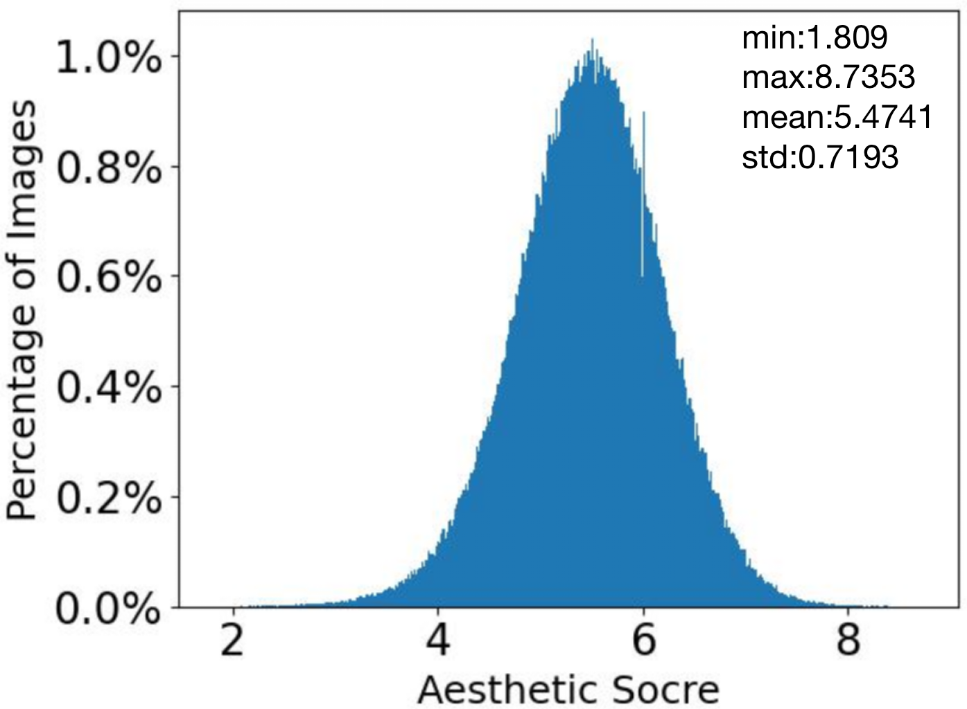
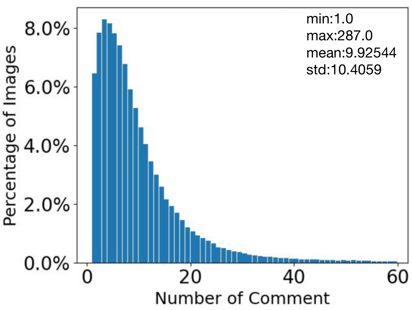
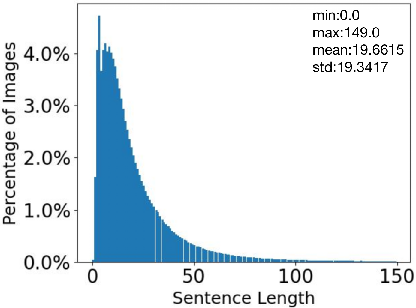
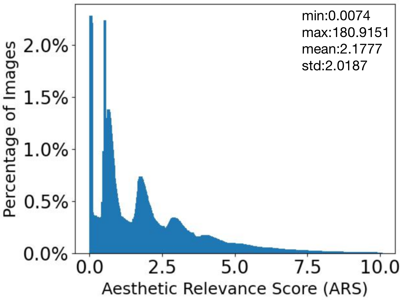
Figure 1: Basic statistics of the DPC2022 dataset.

Image Aesthetic Relevance of Text

The dictionary definition of aesthetic is “concerned with beauty or the appreciation of beauty”, this is a vague and subjective concept. Photographers often use visual characteristics such as lighting, composition, subject matter and colour schemes to create aesthetic photos. Comments associated with images, especially those on the internet websites, can refer to a variety of topics, not all words are relevant to the aesthetics of images, and some words may be more relevant than others. To the best of the authors’ knowledge, there exist no definitions of image aesthetic relevant words and phrases in the computational aesthetic literature. And yet when inspecting the comments from the DPC2022 dataset, it is clear that many have nothing to do with the images’ aesthetic qualities. It is therefore appropriate to distinguish words that refer to the aesthetic quality and those that are not relevant. We have developed the Aesthetic Relevant Score (ARS) to quantify a comment’s aesthetic relevance. It is based on a mixture of subjective judgement and statistics from the dataset. Before describing the ARS in detail, it is appropriate to note that this is by no means the only way to define such a quantity, however, we will demonstrate its usefulness through application in image aesthetic captioning and multi-modal image aesthetic quality assessment.

Labelling a Sentence with its ARS

The ARS of a sentence $t$ is defined as:

$$ARS(t)=A(t)+L(t)+O(t)+S(t)+T_{fidf}(t)$$ (1)

where $A(t)$ is related to aesthetic words, $L(t)$ is related to the length of $t$, $O(t)$ is related to object words, $S(t)$ is the sentiment score of $t$, and $T_{fidf}(t)$ is related to term frequency–inverse document frequency.

The components in (1) are computed based on statistics of the DPC2022 database and details of the computational procedures are in Appendix I in the supplementary materials. For computing $A(t)$, we manually selected 1022 most frequently appeared image aesthetics related words such as shot, color, composition, light, focus, background, subject, detail, contrast, etc., the full list of these words, $\{AW_{list}\}$, can be found in Appendix II. For computing $O(t)$, we manually selected 2146 words related to objects such as eye, sky, face, ribbon, water, tree, flower, expression, hand, bird, glass, dog, hair, cat, smile, sun, window, car, etc, the full list of these words, $\{OW_{list}\}$, can be found in Appendix III. The sentiment score $S(t)$ is calculated based on the $BerTweet$ model (Pérez, Giudici, and Luque 2021). Figure 1(d) shows the distribution of ARS of the DPC2022 dataset. It is seen that many sentences contain no aesthetic relevant information, and the majority of the comments contain very low aesthetic relevant information. Informally inspecting the data shows that this is reasonable and expected.

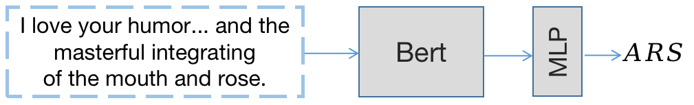
Figure 2: ARS Predictor

.

Automatically Predicting the ARS

For the ARS to be useful, we need to be able to predict any given text’s aesthetic relevant score. With the labelled data described above, we adopt the pre-trained Bidirectional Encoder Representations (BERT) language representation model (Devlin et al. 2018) for this purpose. A $768\times 1$ fully connected layer is cascaded to the output of BERT as shown in Figure 2. We train the model with the mean squared error (MSE) loss function. Table 1 shows the ARS prediction performance. It is seen that the Spearman’s rank-order correlation (SRCC) and the Pearson linear correlation coefficient (PLCC) are both above 0.95, indicating excellent prediction accuracy. It is therefore possible to predict a sentence’s ARS with an architecture shown in Figure 2.

Metrics	SRCC$\uparrow$	PLCC$\uparrow$	RMSE$\downarrow$	MAE$\downarrow$
Performance	0.9553	0.9599	0.5617	0.3395

Table 1: ARS prediction accuracy.

Aesthetically Relevant Image Captioning

Image Captioning Model

For image captioning, many models based on LSTM (Vinyals et al. 2014) and Transformer (Vaswani et al. 2017) have been developed. Given an image, we first extract visual features using an encoder structure, then use a decoder to generate image captions as shown in Figure 3. To obtain image embedding, we follow the bottom-up-attention model (Anderson et al. 2018) and use ResNet-101 (He et al. 2016) as the backbone network of the Faster R-CNN (Ren et al. 2015) to extract image features. The bottom-up attention model uses a region proposal network (RPN) and a region-of-interest (ROI) pooling strategy for object detection. In this paper, we retain 50 most interesting regions and pass them to the encoder for image caption generation. Each region is represented by a 2048-dimensional feature vector.

For the decoder, we use VisualGPT (Chen et al. 2022) to generate image aesthetic captions. VisualGPT is an encoder-decoder transformer structure based on GPT-2 (Radford et al. 2019) which is a powerful language model but does not have the ability to understand images. VisualGPT uses a self-resurrecting activation unit to encode visual information into the language model, and balances the visual encoder module and the language deocder module.

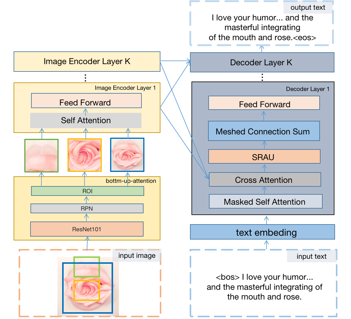
Figure 3: Image captioning model. Left: object detection is performed on the input image, visual features and positions of the regions of interest are encoded. Right: image caption is generated based on the encoded image features. Note the input text is paired with the input image for training purpose.

Aesthetically Relevant Loss Function

Unlike general image captioning which in most cases is about revealing the content and semantics of the image, e.g., objects in the image and their relations, image aesthetic captioning (IAC) should focus on learning aesthetically relevant aspects of the image. Arguably, IAC is much more challenging than generic image captioning. The very few existing IAC related literature, e.g., (Chang, Lu, and Chen 2017), (Jin et al. 2019) and (Ghosal, Rana, and Smolic 2019), simply treat the raw image comments from the training data as the IAC ground truth. However, as discussed previously, many of the texts contain no or very low aesthetic relevant information. The ARS($t$) quantitatively measures the aesthetic relevance of a piece of text $t$, a higher ARS($t$) indicates that $t$ contains high aesthetic relevant information and a low ARS($t$) indicates otherwise. We therefore use ARS($t$) to define the aesthetically relevant loss function to construct the IAC model.

Given training set $\{T(k)\}=\{I,y^{*}(t_{k})\}$ which contains pairs of input image $I$ and one of its corresponding ground-truth caption sentences $y^{*}(t_{k})=(y_{1}^{*}(t_{k}),y_{2}^{*}(t_{k}),...,y_{N_{k}}^{*}(t_{k}))$ consisting of words $y_{i}^{*}(t_{k})$, $i=1,2,...,N_{k}$, we generate a caption sentence $y(t_{k})=(y_{1}(t_{k}),y_{2}(t_{k}),...,y_{N_{k}}(t_{k}))$ that maximises the following ARS($t$) weighted cross-entropy loss

$$L_{AR}(\theta)=-\sum_{k=1}^{k=|T|}ARS(t_{k})\sum_{i=1}^{N_{k}}\mathrm{log}~{}p\left(y_{i}(t_{k})=y_{i}^{*}(t_{k})|\bm{\theta}\right)$$ (2)

where $t_{k}$ is the $k^{th}$ training sentence (note one image $I$ can have multiple sentences), $|T|$ is the training set size (in terms of sentences), $N_{k}$ is the number of words in the $k^{th}$ training sentence, and $\bm{\theta}$ is the model parameters.

Diverse Aesthetic Caption Selector (DACS)

Traditional IAC models such as the one described in Figure 3 output sentences based on the generator’s confidence. All existing methods in the literature (Chang, Lu, and Chen 2017), (Jin et al. 2019) and (Ghosal, Rana, and Smolic 2019) adopt this approach. However, the generator’s confidence is not directly based on aesthetic relevance. The new ARS concept introduced in this paper has provided a tool to measure the aesthetic value of a sentence, which in turn can help selecting aesthetically more relevant and more diverse captions from the generator.

Based on the ARS score defined in (1) for a piece of text $t$, we design a sentence selector method that enables the IAC model to generate diverse and aesthetically relevant sentences. Given a picture, we use the IAC model and beam search (Olive, Christianson, and McCary 2011) to generate $N$ most confident sentences. Then we use a sentence transformer to extract the features of the sentences, and then calculate the cosine similarity among the $N$ sentences. We group sentences whose cosine similarity is higher than 0.7 into the same group such that each group contains many similar sentences. Then, we use the ARS predictor in Figure 2 to estimate the ARS of the sentences in each group. If the average ARS of a group’s sentences is below the mean ARS of the training data ($2.1787$), then the group is discarded because their aesthetic values are low. From the remaining groups, we then pick the sentence with the highest ARS in each group as the output. With this method, which we call the Diverse Aesthetic Caption Selector (DACS), we generate aesthetically highly relevant and diverse image captions. In the experiment section, we will show that OpenAI’s CLIP (Radford et al. 2021), a powerful image and text embedding model that can be used to find the text snippet best represents a given image, can be fine tuned to play the role of ARS for picking the best sentence in a group as output.

Multi-modal Aesthetic Quality Assessment

The purposes of performing multi-modal AQA are two folds. Firstly, the newly established DPC2022 is one of the largest publicly available datasets and quite unique in the sense that it contains both comments and aesthetic scores. We want to provide some AQA performance baselines. Secondly, we make the reasonable assumption that the more accurate a piece of text can predict an image’s aesthetic rating, the more aesthetically relevant is the text to the image.

The image AQA model is shown in Figure 4. There are 3 separate paths. The first takes the image as input and output the image’s aesthetic rating. A backbone neural network is used for feature extraction. The features are then fed to an MLP to regress the aesthete rating. The second path takes the textual description of the image as input and output the image’s aesthetic score. Again, a neural network backbone is used for textual feature extraction. The features are fed to an MLP network to output the aesthetic score. The third path is used to implement multi-modal AQA where visual and textual features are concatenated and fed to a MLP to output the aesthetic score.

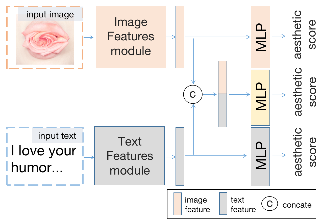
Figure 4: Multi-modal Image Aesthetic Quality Assessment.

Experimental Results

We perform experiments based on the newly constructed DPC2022 dataset. It has a total of 510,000 photos where each photo also contains a review text. 350,000 out of the 510,000 photos also have aesthetic ratings. We call the dataset containing all images setA, and the subset containing images with both reviews and aesthetic ratings SetB. We use SetA for photo aesthetic captioning experiment and SetB for multi-modal aesthetic quality assessment. We divide SetB into a test set containing 106,971 images and a validation set containing 10,698 images, and the remaining 232,331 images are used as the training set. In photo aesthetic captioning, we use the same test set and validation set as those used in multi-modal aesthetic quality assessment, and the remaining SetA data (392,331 images) is used for training.

Evaluation Criteria

Similar to those in the literature, we use 5 metrics to measure the performance of image AQA including Binary Accuracy (ACC), Spearman rank order correlation coefficient (SRCC), Pearson linear correlation coefficient (PLCC), root mean square error (RMSE), and mean absolute error(MAE). For image captioning, we use 4 metrics widely used in related literature including CIDER (Vedantam, Lawrence Zitnick, and Parikh 2015), METETOR (Banerjee and Lavie 2005), ROUGE (Lin 2004), and SPICE (Anderson et al. 2016). SPICE is a word-based semantic similarity measure for scene graphs, and the others are all based on n-gram.

Implementation Details

For image based AQA, we have used VGG-16, RESNET18, DESNET121, RESNEXT50, and ViT (Dosovitskiy et al. 2020) as the backbone network and used their pre-trained models rather than training from scratch. The images are resized to 224x224, randomly flipped horizontally, and normalised to have a mean of 0.5 and a variance 0.5. For text based AQA, we have used the TEXTCNN (Kim 2014), TEXTRNN (Lai et al. 2015), BERT (Devlin et al. 2018) and ROBERTA (Liu et al. 2019)) as the backbone network. For BERT and ROBERTA, we use their pre-trained models. Finally, we limit the number of tokens for each image’s comment to 512. For IAC, we used the pre-trained GPT2 model and set token size to 64. All experiments were performed on a machine with 4 NVIDIA A100 GPUs. Adam optimizer with a learning rate of $2e^{-5}$ without weight decay was used. The AQA models were trained for 16 epochs and the IAC models were trained for 32 epochs. Codes will be made publicly available.

Image AQA Baseline Results

In the first set of experiments, we experimented various network architectures in order to obtain some baseline image AQA results. Table 2 lists the baseline results of image based, text based, and mutlti-modal AQA results when the backbone used different network architectures. These results show that the textual reviews of the images are aesthetically highly relevant. In two out of 5 metrics, using the review text only gives the best performances. It is also seen that in 3 other metrics, multi-modal AQA has the best performances.

Backbone	ACC$\uparrow$	SRCC$\uparrow$	PLCC$\uparrow$	RMSE$\downarrow$	MAE$\downarrow$
Image based AQA
VGG16	0.7848	0.5914	0.6078	0.5977	0.4699
RESNET18	0.8007	0.5946	0.6108	0.5850	0.4588
DESNET121	0.8096	0.6331	0.6471	0.5501	0.4287
RESNEXT50	0.8067	0.6386	0.6530	0.5486	0.4282
ViT	0.8194	0.6755	0.6868	0.5356	0.4193
Text based AQA
TEXTCNN	0.812	0.6069	0.6251	0.461	0.5891
TEXTRCNN	0.8665	0.7516	0.7730	0.3611	0.4649
BERT	0.8810	0.8024	0.8219	0.3292	0.4235
ROBERTA	0.8939	0.8334	0.8551	0.2988	0.3826
Multi-modal (image plus text) AQA
RESNEXT50+RNN	0.8591	0.8289	0.8456	0.3864	0.2998
RESNEXT50+BERT	0.8666	0.8493	0.8695	0.3780	0.2941
ViT+RNN	0.8622	0.8386	0.8537	0.3747	0.2901
ViT+ROBERTA	0.8693	0.8629	0.8803	0.3545	0.2756
ViT+BERT	0.8697	0.8594	0.8766	0.3604	0.2814

Table 2: AQA baseline results of DPC2022

Data Group	ACC$\uparrow$	SRCC$\uparrow$	PLCC$\uparrow$	RMSE$\downarrow$	MAE $\downarrow$
All	0.8666	0.8657	0.8814	0.3688	0.2883
Low $A$	0.8497	0.8247	0.8403	0.3725	0.2907
High $A$	0.8966	0.9150	0.9193	0.3621	0.2841
Low $O$	0.8516	0.8335	0.8498	0.3714	0.2903
High $O$	0.8954	0.908	0.9127	0.3639	0.2845
Low $L$	0.8521	0.8238	0.837	0.3704	0.2895
High $L$	0.8944	0.9184	0.9213	0.3658	0.2860
Low $S$	0.8358	0.814	0.8274	0.375	0.2937
High $S$	0.9300	0.9015	0.9144	0.3557	0.2773
Low $T_{fidf}$	0.8502	0.8182	0.8332	0.3714	0.2908
High $T_{fidf}$	0.8898	0.9107	0.9146	0.3651	0.2849
Low $ARS$	0.8486	0.8216	0.8352	0.3726	0.2910
High $ARS$	0.8991	0.9157	0.9202	0.3620	0.2835

Table 3: Multi-modal AQA for images with high and low aesthetic relevant comments. These results are all based on VIT+BERT model.

ARS Threshold	ACC$\uparrow$	SRCC$\uparrow$	PLCC$\uparrow$	RMSE$\downarrow$	MAE $\downarrow$
$ARS\leq m_{ARS}-1.0\sigma_{ARS}$	0.8070	0.5992	0.6443	0.4252	0.3298
$ARS\leq m_{ARS}-0.8\sigma_{ARS}$	0.8213	0.6969	0.7172	0.3985	0.3079
$ARS\leq m_{ARS}-0.6\sigma_{ARS}$	0.8350	0.7602	0.7755	0.3848	0.3003
$ARS\leq m_{ARS}-0.4\sigma_{ARS}$	0.8415	0.7948	0.8091	0.3761	0.2940
$ARS\leq m_{ARS}-0.2\sigma_{ARS}$	0.8446	0.8105	0.8231	0.3750	0.2931
$ARS\leq m_{ARS}-0.0\sigma_{ARS}$	0.8486	0.8216	0.8352	0.3726	0.2910
$ARS\geq m_{ARS}+0.0\sigma_{ARS}$	0.8991	0.9157	0.9202	0.3620	0.2835
$ARS\geq m_{ARS}+0.2\sigma_{ARS}$	0.9098	0.9206	0.9248	0.3626	0.2836
$ARS\geq m_{ARS}+0.4\sigma_{ARS}$	0.9129	0.9244	0.9261	0.3662	0.2863
$ARS\geq m_{ARS}+0.6\sigma_{ARS}$	0.9183	0.9274	0.9280	0.3652	0.2835
$ARS\geq m_{ARS}+0.8\sigma_{ARS}$	0.9237	0.9280	0.9291	0.3670	0.2852
$ARS\geq m_{ARS}+1.0\sigma_{ARS}$	0.9232	0.9294	0.9291	0.3667	0.2854
ungroup(all)	0.8666	0.8657	0.8814	0.3688	0.2883

Table 4: Multi-modal image AQA. As the ARS of the comment texts increases, the aesthetic rating prediction performances increases. $m_{ARS}$ is the mean of ARS and $\sigma_{ARS}$ is the variance of the ARS of the DPC2022 dataset. $ARS\leq m_{ARS}-\alpha\sigma_{ARS}$ indicates the group of images each with a comment having an ARS value less than or equal to $m_{ARS}-\alpha\sigma_{ARS}$.

Verification of ARS

To verify the soundness of the newly introduced ARS, we divide the DPC2022 validation set into two groups according to the ARS. If the ARS model is sound, then we would expect a review text with a higher ARS should be able to predict the image’s aesthetic rating more accurately. Conversely, a review text that has a lower ARS would produce a less accurate prediction of the image’s aesthetic rating. Table 3 shows the multi-modal AQA performances for two groups of testing samples. Low $ARS$ ($A,O,L,S,T_{fidf}$) represent the group where test samples have a $ARS$ ($A,O,L,S,T_{fidf}$) lower than their respective average values. High $ARS$ ($A,O,L,S,T_{fidf}$) represent the group where test samples have a $ARS$ ($A,O,L,S,T_{fidf}$) higher than their respective average values. Table 4 shows that as the ARS increases, so does the AQA performances. These results clearly show that comments with high ARS can consistently predict the images aesthetic rating more accurately than those with low ARS. This means that ARS and its components can indeed measure the aesthetic relevance of textual comments.

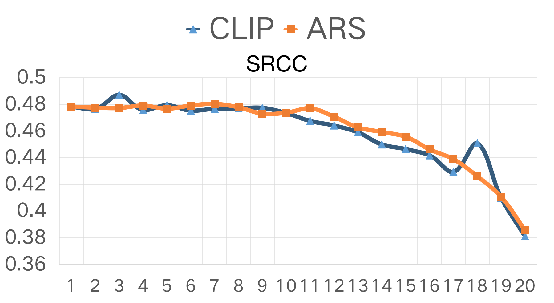
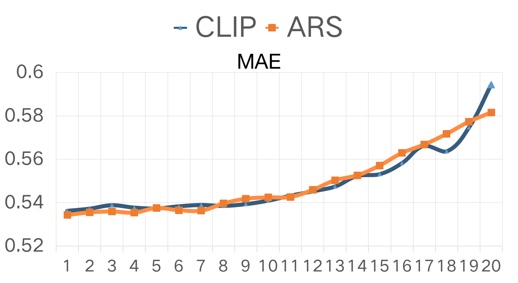
Figure 5: Comparison between CLIP and ARS for ranking aesthetically relevant sentences for image AQA. Horizontal-axis is the rank position.

ARS versus CLIP for Ranking Text Relevance

CLIP (Contrastive Language-Image Pre-Training) is a neural network trained on a variety of (image, text) pairs (Radford et al. 2021). It is a powerful model that can match natural language descriptions with visual contents. In this experiment, we first fine tune the pre-trained CLIP model with the training set of the DPC2022 data such that the images and their corresponding comments are matched. With such a fine tuned model, we can rank the sentences in the comments of the images. Let CLIP$(I,t)$ be the matching score between an image $I$ and a sentence $t$. Suppose we have two sentences $t_{i}$ and $t_{j}$, if CLIP$(I,t_{i})>$ CLIP$(I,t_{j})$ then $t_{i}$ and $I$ is a better match. Because CLIP has been fine tuned on DPC2022, it is reasonable to assume that if a text and an image has a better CLIP matching score, then the text can describe the image more accurately. Similar to ARS, we can use CLIP to rank the sentences according to their CLIP matching scores. To compare the CLIP and ARS in the selection of texts for image AQA, we rank the sentences of the images in the test set and perform text based AQA for the sentences in different ranks. The SRCC and MAE performances of those ranked by ARS and CLIP are shown in Figure 5. It is seen that the higher ranking sentences by both methods can predict the aesthetic rating more accurately, and that both seem to perform very similarly. These results show that the properly fine tuned CLIP model can also be used to select aesthetically relevant text for image AQA. It is worth noting that ARS is a very simple scheme while CLIP is a much more complex but powerful model. Figures 6 shows visual examples of how the sentences are ranked by ARS and CLIP.

Aesthetic Captioning Performances

Table 5 shows the aesthetic image captioning performances of our new aesthetically relevant model (ARIC) based on the loss function $L_{AR}(\theta)$ as defined in (2). For comparison, we have implemented a baseline model in which standard cross entropy loss function is used, i.e., setting $ARS(t_{k})=1$ in (2). It is seen that our new model consistently outperforms the baseline model. These results demonstrate the usefulness and effectiveness of introducing the aesthetically relevant score (ARS) for aesthetics image captioning. Even though these metrics do not directly measure aesthetic relevance, the better performances of the new method nevertheless demonstrate the soundness of the new algorithm design.

As described in the main method, with the introduction of ARS, we can use ARS based diverse aesthetic caption selector (DACS) to generate a diverse set of image captions rather than being restricted to output only one single sentence as in previous methods (Chang, Lu, and Chen 2017). Figures 6 shows examples of aesthetic captions generated with ARS based and CLIP based DACS. More examples are available in the Supplementary materials.

Methods	METETOR $\uparrow$	ROUGE(L) $\uparrow$	CIDER$\uparrow$	SPICE$\uparrow$
Baseline	0.1227	0.3543	0.0580	0.0172
ARIC (2)	0.1389	0.3610	0.0633	0.0353

Table 5: Image aesthetic captioning performances of our new model as compared with the baseline model.

Method	ACC$\uparrow$	SRCC$\uparrow$	PLCC$\uparrow$	RMSE$\downarrow$	MAE $\downarrow$
Image only	0.8194	0.6755	0.6868	0.5356	0.4193
AQA using Ground Truth Text
Text only	0.8533	0.8274	0.851	0.3828	0.2960
Multi-modal(Image+Text)	0.8407	0.7529	0.7691	0.4650	0.3659
AQA using Generated Captions
Text only Traditional	0.7630	0.4335	0.4269	0.8921	0.7152
Text only DACS (ARS)	0.7695	0.4711	0.4693	0.7881	0.6227
Text only DACS (CLIP)	0.7720	0.476	0.4745	0.7645	0.6018
Multi-modal Traditional	0.8181	0.6818	0.6925	0.5422	0.4232
Multi-modal DACS (ARS)	0.8195	0.6833	0.6934	0.5357	0.4192
Multi-modal DACS (CLIP)	0.8203	0.6837	0.6940	0.5340	0.4179

Table 6: Image AQA using generated captions. Traditional: no aesthetic relevance selection where all generated sentences are used. DACS(ARS): using sentences selected by the ARS based diverse aesthetic caption selector (DACS). DACS(CLIP): using sentences selected by the CLIP based diverse aesthetic caption selector (DACS).

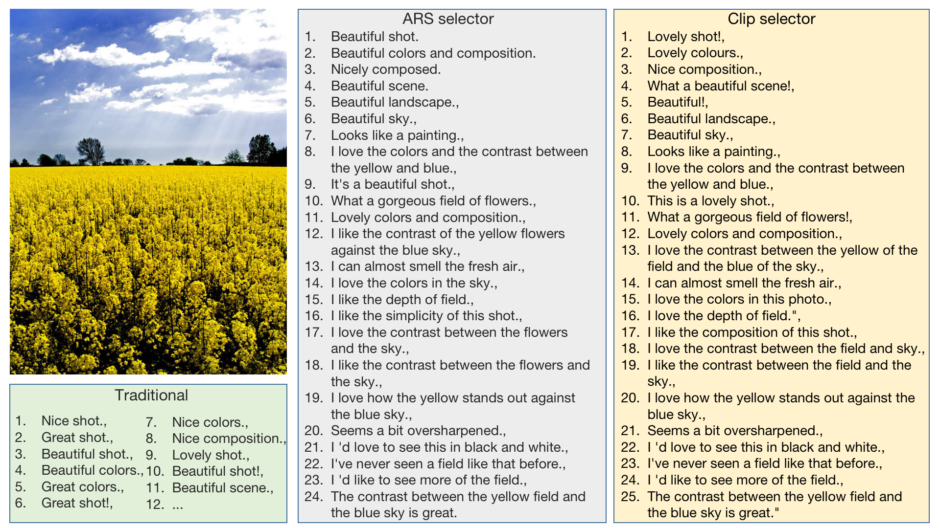
Figure 6: Example captions. Traditional: The sentences are ranked based on the generator’s confidence without using the DACS. ARS selector: ARS is used to construct the DACS and pick the generated sentences according to ARS values. CLIP selector: the fine tuned CLIP model is used to rank the generated sentences to construct the DACS and pick the sentences according to the CLIP matching scores. Note CLIP is only used to pick the best sentence in a group as one of the output sentences of DACS. It is seen that with DACS, the captions are more diverse. More example results are available in the Supplementary materials.

Image AQA based on Generated Captions

In this experiment, we evaluate image AQA performances based on the generated image captions and results are shown in Table 6. We can observe that in text only AQA, the generated texts perform worse than the true captions, and also worse than image only AQA. It is also seen that using captions selected by the new diverse aesthetic caption selector (DACS) either based on ARS or CLIP performs better than using captions without selection. It is interesting to observe that in multi-modal AQA, including the generated texts has started to slightly exceed image only AQA, but is still quite far from those using ground truth. For example, using ground truth text, the ACC of multi-modal AQA is 0.8407 whilst that using generated captions is 0.8203. Would a future image captioning model be able to generate captions to close the gap? This would be a very interesting question and a goal for future research.

Concluding Remarks

In this paper, we have attempted to study two closely related subjects of aesthetic visual computing, image aesthetic quality assessment (AQA) and image aesthetic captioning (IAC). We first introduce the concept of aesthetic relevance score (ARS) and use it to design the aesthetically relevant image captioning (ARIC) model through an ARS weighted loss function and an ARS based diverse aesthetic caption selector (DACS). We have presented extensive experimental results which demonstrate the soundness of the ARS concept and the effectiveness of the ARIC model. We have also contributed a large research database DPC2022 that contains images with both comments and aesthetic ratings.

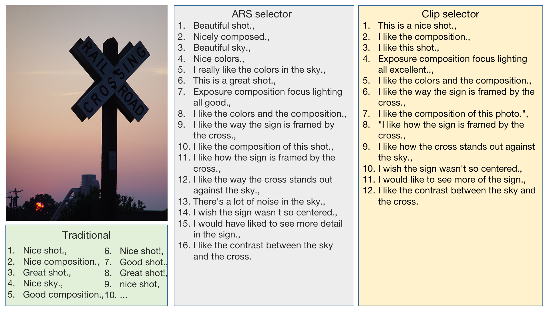
Figure 7: More examples

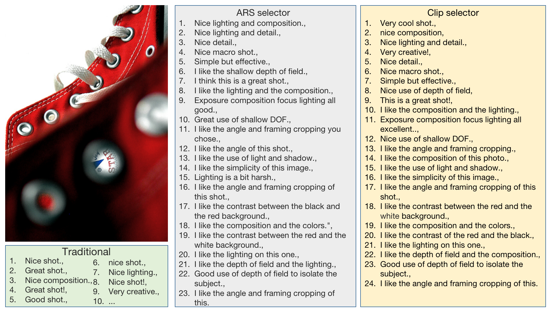
Figure 8: More examples

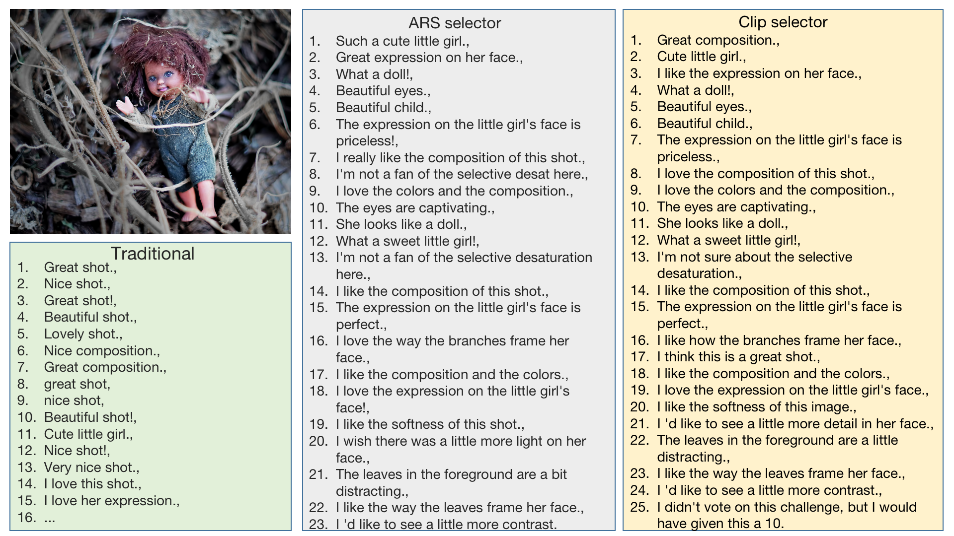
Figure 9: More examples

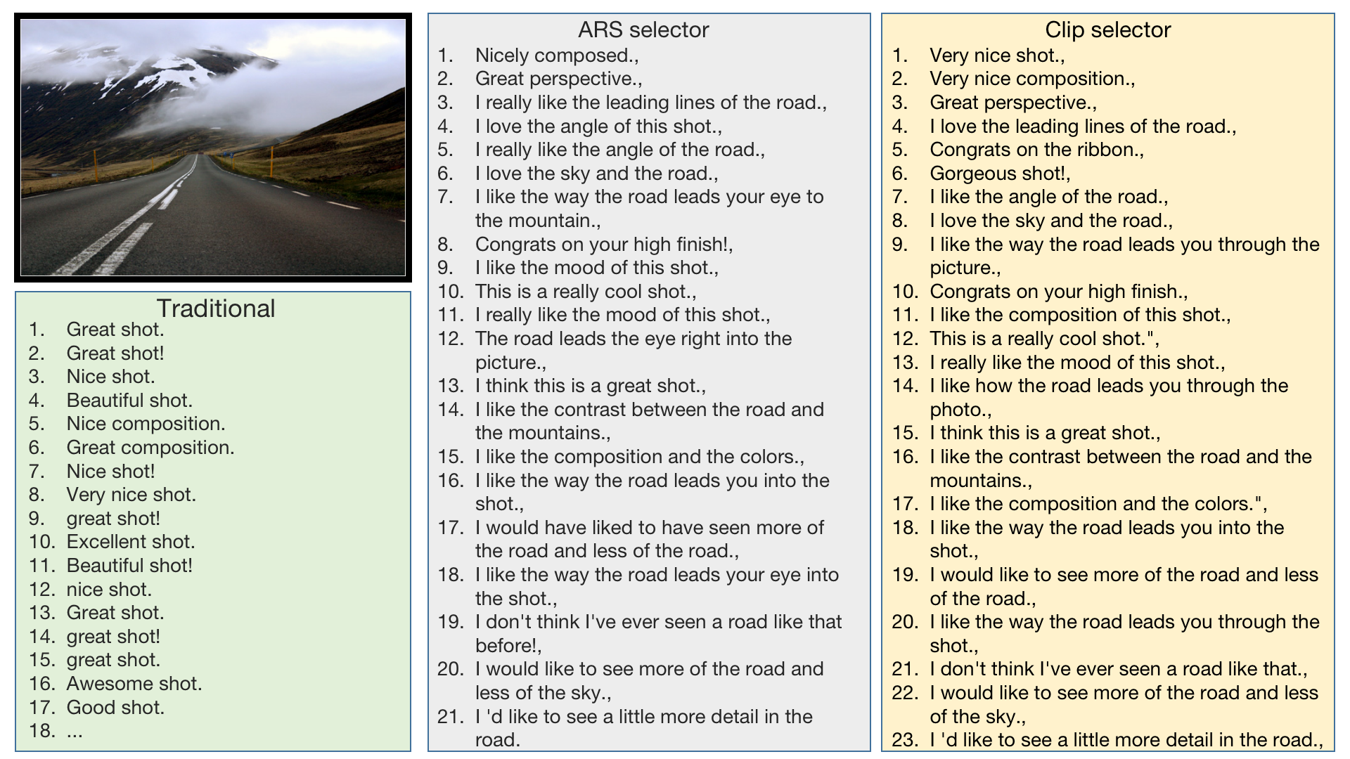
Figure 10: More examples

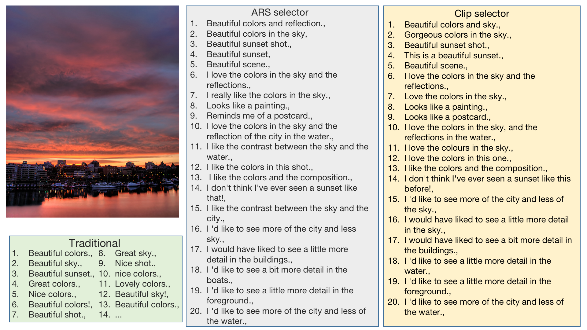
Figure 11: More examples

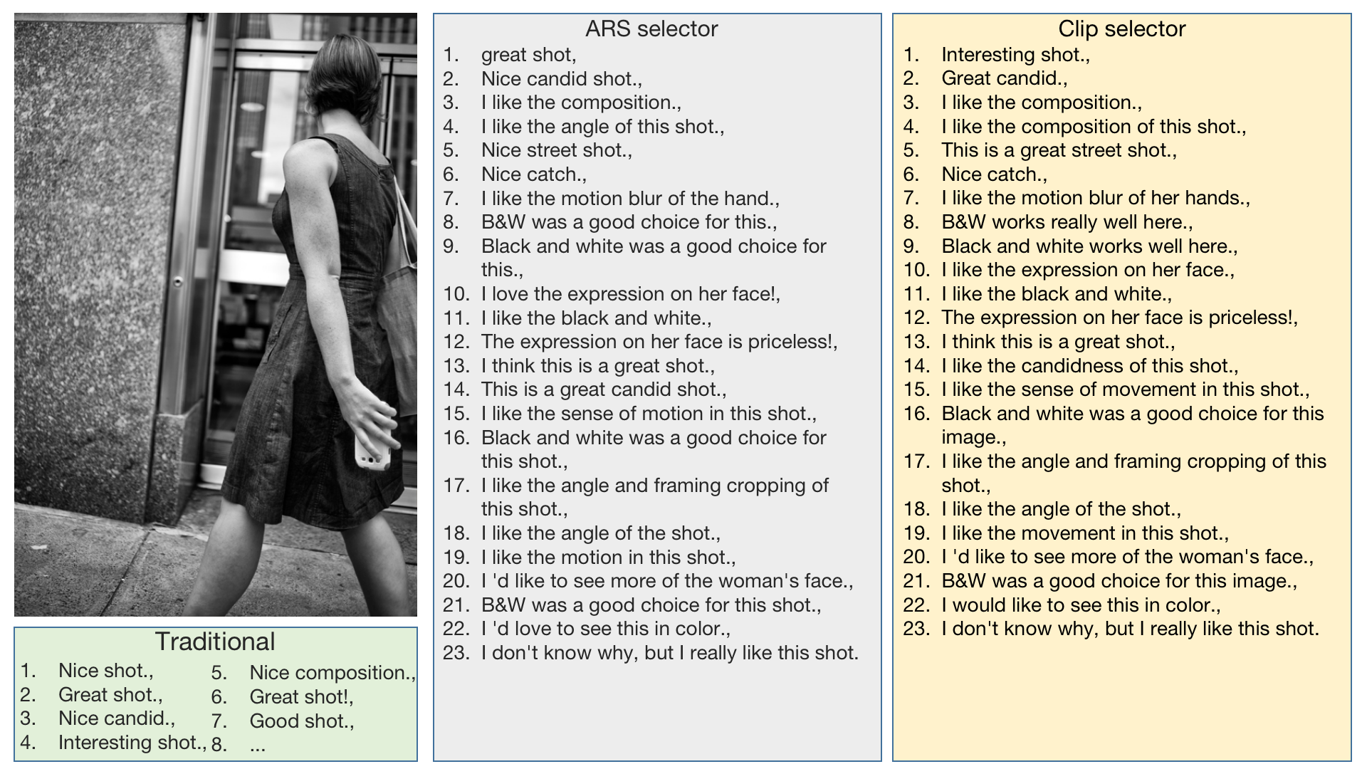
Figure 12: More examples

Appendix A Appendix I

The ARS of a sentence $t$ is defined as:

$$ARS(t)=A(t)+L(t)+O(t)+S(t)+T_{fidf}(t)$$ (3)

where $A(t)$ is related to aesthetic words, $L(t)$ is related to the length of $t$, $O(t)$ is related to object words, $S(t)$ is the sentiment score of $t$, and $T_{fidf}(t)$ is related to term frequency–inverse document frequency.

We first counted the nouns, adverbs, adjectives, and verbs of all comments, sorted by word frequency from high to low. We manually selected 1022 most frequently appeared image aesthetics related words, the full list, $\{AW_{list}\}$, can be found in Appendix II. We also manually selected 2146 words related to objects, the full list of these words, $\{OW_{list}\}$, can be found in Appendix III.

To obtain the $A(t)$, we simply count how many of these 1022 words have appeared in $t$

$$A(t)=\sum_{w=1}^{w=|t|}\delta_{a}(t_{w}),$$ (4)

where $t_{w}$ is the $w^{th}$ word in $t$, $|t|$ is the length of $t$, $\delta_{a}(t_{w})=1$ if $t_{w}\in AW_{list}$ and $\delta_{a}(t_{w})=0$ otherwise.

$L(t)$ is calculated as

$$L(t)=\frac{\beta(|t|,m_{|t|},\sigma_{|t|})-\beta(|t|_{min},m_{|t|},\sigma_{|t|})}{\beta(|t|_{max},m_{|t|},\sigma_{|t|})-\beta(|t|_{min},m_{|t|},\sigma_{|t|})}$$ (5)

where $|t|$ is the length (number of words) of $t$, $m_{|t|}$ is the average length of sentences, $\sigma_{|t|}$ is the variance of the length of the sentences, $|t|_{max}$ is the length of the longest sentence and $|t|_{min}$ is the length of the shortest sentence in the dataset, and $\beta$ is a sigmoid function defined in (6)

$$\beta(x,m,\sigma)=\frac{1}{1+e^{-(\frac{x-m}{\sigma})}}$$ (6)

$O(t)$ is calculated as

$$O(t)=\sum_{w=1}^{w=|t|}\delta_{o}(t_{w})$$ (7)

where $t_{w}$ is the $w^{th}$ word in $t$, $|t|$ is the length of $t$, $\delta_{o}(t_{w})=1$ if $t_{w}\in OW_{list}$, and $\delta_{o}(t_{w})=0$ otherwise.

$S(t)$ is the sentiment score of $t$. We used the $BerTweet$ model and the toolkit from(Pérez, Giudici, and Luque 2021) to calculate both the positive and negative sentiments of $t$ and obtain $S(t)$ as

$$S(t)=\frac{P_{s}(t)+N_{s}(t)}{2}$$ (8)

where $P_{s}(t)$ is the predicted positive sentiment and $N_{s}(t)$ is the predicted negative sentiment of $t$, and the values of both $P_{s}(t)$ and $N_{s}(t)$ are in $[0,1]$.

$T_{fidf}(t)$ is related to term frequency-inverse document frequency (tf-itf). For a give term tm, we first calculate its tf-itf value $\tau(tm)$

$$\tau(tm)=\frac{n_{tm}}{N_{tm}}*\left(log\left(\frac{1+N}{1+I_{tm}}\right)+1\right)$$ (9)

where $n_{tm}$ is the number of times the term $tm$ has appeared in the comment of a given image, $N_{tm}$ is the total number of terms in the comment of the image, $N$ is the total number of images in the dataset, and $I_{tm}$ is the number of images with comments containing the term $tm$. We then normalise $\tau(tm)$ according to

$$\tau_{n}(tm)=\frac{\beta(\tau(tm),m_{\tau(tm)},\sigma_{\tau(tm)})-\beta_{min}(\tau(tm))}{\beta_{max}(\tau(tm))-\beta_{min}(\tau(tm))}$$ (10)

where $\beta_{min}(\tau(tm))=\beta(\tau_{min}(tm),m_{\tau(tm)},\sigma_{\tau(tm)})$, $\beta_{max}(\tau(tm))=\beta(\tau_{max}(tm),m_{\tau(tm)},\sigma_{\tau(tm)})$, $\tau_{min}(tm)$ is the smallest $\tau(tm)$, $\tau_{max}(tm)$ is the largest $\tau(tm)$, $m_{\tau(tm)}$ is the mean value and $\sigma_{\tau(tm)}$ is the variance of $\tau(tm)$ of the dataset.

Finally, we compute the $T_{fidf}(t)$ in equation (1) as

$$T_{idf}(t)=\sum_{i=1}^{i=|t|}\tau_{n}(tm(i))$$ (11)

where $tm(i)$ is the $i^{th}$ term, $|t|$ is the length of $t$.

Appendix II: Aesthetic word table, 1/2
shot	color	composition	light	focus	lighting	background	subject
right	detail	shoot	contrast	crop	colour	tone	white
blue	dark	line	texture	angle	shadow	sharp	frame
black	high	left	reflection	soft	point	post	red
perspective	overall	distract	leave	strong	bright	creative	scene
exposure	low	camera	simple	green	blur	view	space
away	concept	border	catch	foreground	depth	long	small
abstract	spot	center	yellow	motion	area	tight	draw
lack	shape	moment	lead	neat	attention	miss	dof
balance	quality	field	mood	sharpness	element	distracting	edge
highlight	theme	level	compose	end	stop	corner	art
rest	flat	framing	tilt	pattern	bokeh	lens	cut
large	move	unique	blurry	horizon	rule	noise	silhouette
warm	grain	shallow	movement	middle	curve	size	pull
orange	cropping	saturation	sharpen	expose	fill	emotion	odd
couple	grainy	range	cover	style	sepia	similar	position
focal	shutter	softness	simplicity	half	branch	suggest	pink
imagine	hot	filter	overexposed	match	body	form	brown
classic	diagonal	distraction	remove	purple	square	impressive	reflect
colorful	stick	smooth	blend	combination	location	shade	mirror
layer	vertical	impression	snapshot	centered	desat	darkness	suit
overlay	aspect	single	grey	tonal	flow	hue	connection
base	entire	blurred	higher	symmetry	part	gray	distance
coloring	saturate	backdrop	scale	noisy	surface	balanced	emotive
horizontal	cross	structure	golden	rotate	atmosphere	direction	context
outside	fade	btw	aperture	gold	pure	pixel	thread
wire	centre	bunch	fuzzy	film	profile	focused	toning
mask	environment	desaturation	mystery	inside	portion	side	mysterious
crowd	mix	b&w	duotone	order	addition	colored	emotional
iso	underexposed	central	underrated	bg	architecture	ray	oversharpened
pastel	detailed	surround	group	mess	combine	apart	aside
sport	narrow	cluttered	tint	band	spirit	desaturate	distortion
darken	artifact	compression	dimension	compostion	closeup	upside	major
compositionally	positioning	contrasty	repeat	fork	tall	lay	triangle
reference	juxtaposition	condition	surrounding	shooting	ripple	weak	belong
lighten	placing	connect	ghost	warmth	pair	row	viewpoint
sight	lightning	stripe	backlighting	clue	top	minimalism	colourful
intensity	continue	hdr	soften	brighten	orientation	layout	lower
tonality	outline	rotation	obscure	sensor	lense	oversaturated	height
blind	resolution	artificial	fisheye	palette	parallel	geometry	cropped
crooked	silver	partial	combo	overprocessed	makeup	offset	streak
patch	wrinkle	resize	concentrate	minimalist	symmetrical	saturated	backround
length	raw	monochrome	coloration	misty	criterion	tightly	uneven
up	hazy	rhythm	pale	oversharpene	relationship	panning	recommend
graininess	constructive	rear	textured	forground	geometric	overexposure	blank
unbalanced	posture	unsharp	aesthetic	rim	backlit	channel	interaction
uniform	smoothness	proportion	sentiment	foggy	cloudy	isolation	ratio
speck	cell	colouring	lensbaby	overcast	backlighte	blob	zone
blurring	regular	polarizer	circular	drab	overexpose	bw	back
minimalistic	coloured	compositon	backlight	overhead	abstraction	partially	composite
curved	oversaturate	greenish	reshoot	sharply	slant	spotlight	fore
pix	yellowish	compo	calibrate	cartoon	cone	panoramic	centred
vertically	haloing	align	slope	spiral	interior	monochromatic	vibe
exotic	cube	impressionistic	arrow	sharpening	horizontally	photojournalism	backwards
sized	bluish	pixelate	refraction	monotone	reddish	indoor	greenery
watercolor	ink	cherry	magenta	stance	midtone	blending	mixed
photoshoppe	cyan	toned	nostalgia	whiter	faded	panorama	tinge
underexpose	shot-	overlap	gloomy	focusse	outdoor	runner	container
vista	transparency	tune	lightness	cam	symetry	rectangle	width
shading	aperature	polish	dome	brightly	aesthetically	trim	tuning
pixelated	silhoutte	shadowy	angled	mixture	grid	esque	blurriness
overprocesse	noir	gradation	grayscale	skew	converge	slanted	tan
sphere	blackness	pixelation	compress	trend	straightforward	interplay	unfocused
upwards	emotionally	shadowing	histogram	translucent	comic	bent	impressionist
scatter	shut	gaussian	futuristic	arc	illumination	temperature	radiate
opacity	metaphor	abstractness	alignment	underside	softly	linear	pinkish
vague	textural	void	resizing	ultra	bias	realism	vertigo

Table 7: Aesthetic word table

Appendix II: Aesthetic word table, 2/2
fringe	sharper	silouette	mesh	boundary	barrier	torso	simplify
blurr	artistry	postprocessing	sword	impressionism	span	mapping	romance
backside	silvery	intersect	polarizing	copper	surrealism	juxtapose	diagonally
luminosity	backgound	triangular	contour	solitary	greyscale	whiteness	similarity
symetrical	violet	scope	blueish	amber	compostition	twilight	olive
ambiguous	hanger	vastness	loop	sentimental	indistinct	sillhouette	contrasted
datum	fuzz	dichotomy	curvy	surrealistic	brownish	rectangular	dizzying
blured	shelter	interfere	wavy	shimmer	symmetric	sillouette	shooter
artefact	bleach	smoothing	orb	b+w	blotchy	colortone	gamma
curvature	contrary	blemish	prespective	refection	viewfinder	inclined	oval
cartoonish	restriction	fuzziness	chromatic	fringing	underexposure	lighing	focusing
balancing	bronze	flatness	beige	resemblance	borderline	aqua	contrasting
nighttime	splotch	shaded	perpendicular	radial	masking	radius	verticle
ambiance	bacground	uv	ambience	calibration	swirly	excess	dazzle
hightlight	backgroud	softbox	coil	unbalance	oversharp	detailing	bluer
oversaturation	axis	refract	softening	grayish	purplish	granular	verge
tonemapping	distracted	shutterspeed	tilting	midst	understatement	optic	compressed
perpective	diffusion	treeline	superimpose	shaped	brightening	tendency	askew
lighitng	nuance	specular	refelction	roundness	peacefulness	nothingness	ramp
affection	rigid	similarly	imbalance	coordinate	asymmetrical	reflected	stylize
artifacte	grandeur	skewsme	roughness	greyish	blacker	highlighting	nd
mosaic	camo	silohuette	bound	dof.	oversharpening	buff	rad
colorfull	compozition	fleck	pallette	compsition	silouhette	concentrated	overshadow
asymmetry	variance	geometrical	spacing	mystique	winding	shot–	autofocus
bluey	posed	lightsource	particle	projection	tonemappe	leftmost	compisition
opaque	autumnal	grainyness	incline	deatil	oblique	haziness	rightmost
prism	luminance	reflexion	blueness	criss	colorless	apeture	emerald
apparition	clearness	watercolour	relfection	coordination	redish	balck	colorization
vacant	artifical	straighter	hemisphere	ligthing	colouration	zooming	gimmick
evergreen	backgroung	uniformly	orangy	beneath	uniformity	bleakness	superfluous
reflex	affective	framework	radioactive	mirroring	translucence	epitome	patina
teal	cartoony	tinting	shear	silhouetting	foucs	imaging	polarize
veiw	polariser	texturing	splotchy	midground	crunch	difuse	silhoette
sillouhette	distractingly	foregound	downsize	croping	translucency	postprocesse	peachy
f2.8	800px	visibility	backstory	constitute	storyline	composistion	colors
ligting	boke	sephia	ballance	arched	coposition	overprocessing	spherical
uncropped	highlite	wideangle	hilight	composition-	pixellate	colorize	darkish
spotted	deform	camoflauge	yellowy	orangish	highlighted	harmonize	overlit
colors-	whitebalance	index	oversized	sidelighte	darkest	misplace	speckled
sharpne	backgorund	tilted	brokeh	backgroun	themed	reshot	cleanliness
sharpend	denoise	undertone	diffraction	sihouette	blurri	pixle	pixellation
persepctive	texure	infocus	uncalibrated	focuse	marginal	phantom	composing
noice	comosition	inclination	caliber	matt	higlight	greyness	projector
outlook	megapixel	detial	composotion	horison	polarising	unevenly	clairity
squarish	collor	pixilated	topple	luster	dun	shininess	subect
mauve	dslr	fuzzie	sharpeness	gradiation	discoloration	refelection	colorwise
ccd	chiaroscuro	oversharpen	gradiant	colorized	apperture	sharpener	abberation
shot!	exposer	indigo	exposure(2	bluriness	blurryness	colore	maroon
colourfull	horizion	skiprow	crimson	harmonic	leveling	focus-	glob
despeckle	sigma	unprocessed	feathering	focussing	refinement	resonance	greeny
color-	coppery	quad	blacklight	fidelity	hyperfocal	ghosting	composiiton
telegraph	symetric	persective	dizziness	symmetrically	overlaid	straightness	delineation
beegee	clipping	pallete	compositing	distrace	siloette	reprocess	colrs
quadtone	underlit	antithesis	stripey	streche	taper	colorsaturation	grayness
rightside	grainey	hubcap	unsaturated	speedlight	fuschia	unsharpness	coulour
distrating	geometrically	multicolore	shawdow	pespective	clog	undersaturated	shodow
brink	overexposured	brighness	bakground	tolerant	colourisation	diagnal	coor
middleground	prospect	backgrond	orginality	whitespace	colro	b&w.	ringlight
recroppe	tolerance	balence	granule	perspecitve	disctracte	latex	evenness
defocuse	compositin	light+idea+execution	emo	siloutte	conrast	softfocus	fuzze
deatail	unevenness	croped	compesition	compositiion

Table 8: Aesthetic word table

Appendix III: Object word table, 1/5
eye	sky	face	ribbon	water	tree	flower	expression
people	hand	bird	head	story	sense	glass	guy
man	dog	hair	girl	wall	cat	smile	sun
window	car	rock	crisp	kid	landscape	fall	child
skin	drop	snow	hang	fan	house	book	grass
bridge	ground	painting	horse	sunset	street	road	fence
boat	baby	woman	animal	leg	ball	fly	leaf
boy	shoe	wing	arm	paint	room	bottle	home
mountain	box	wood	star	door	city	moon	plant
smoke	feather	nose	hat	finger	bubble	paper	ice
fire	family	petal	fish	shirt	table	glare	text
card	human	sand	duck	chair	lady	brightness	total
zoom	rain	beach	wave	apple	egg	ring	dress
train	circle	fog	food	land	stone	wind	mouth
floor	ear	bike	halo	flame	butterfly	plane	bee
wheel	cow	portfolio	round	tie	magazine	spider	sea
metal	dust	pencil	pet	kitty	cup	phone	postcard
tower	flag	droplet	statue	weather	neck	hill	toy
shoulder	lamp	energy	candle	lip	rose	mist	board
crack	creature	fur	bar	tail	summer	pan	plastic
sunlight	brick	fruit	trail	church	coffee	drink	rainbow
boot	brush	country	earth	candy	plate	hole	roof
money	music	tack	scenery	material	block	umbrella	tooth
frog	album	urban	milk	bowl	balloon	bench	shell
tear	insect	spring	truck	doll	flight	town	barn
sucker	waterfall	chocolate	artist	garden	bag	dirt	oof
lighthouse	river	dance	beer	guitar	clock	wine	sunrise
lake	vase	button	build	cloth	chain	storm	tongue
clothe	bulb	liquid	alien	ocean	ship	rope	cap
font	stair	park	sheet	bloom	cheese	flaw	wedding
fault	bush	beak	arch	soul	rail	gun	catchlight
crystal	pin	shop	trunk	machine	spoon	knife	seed
sculpture	puzzle	blood	bed	angel	chin	snake	fabric
oil	coat	deer	foliage	woody	ribbone	squirrel	cheek
pepper	toe	puppy	wildlife	cake	seat	ceiling	tv
bud	shoehorn	pool	skyline	curtain	forest	haze	pot
mouse	cream	butt	hammer	coin	swan	clothing	stream
sheep	pier	swirl	outfit	kitchen	jacket	banana	autumn
canvas	steam	yard	lock	vehicle	palm	lemon	pigeon
planet	salt	chicken	critter	stack	tulip	pen	dish
gem	newspaper	cookie	tape	forehead	ant	strawberry	gull
clip	bread	tunnel	needle	artwork	pipe	billboard	berry
knee	fountain	dock	marble	garbage	tomato	cityscape	sugar
chest	bow	spark	bean	horn	sock	cigarette	elephant
straw	screw	pile	glove	mushroom	column	basket	owl
eagle	pumpkin	bunny	pup	cd	net	blanket	anchor
iron	carpet	jewelry	bride	gate	lion	chip	ornament
fishing	dragonfly	kitten	nut	costume	castle	hood	snail
grape	twig	blossom	crisper	stamp	desert	graffiti	beast
railing	windmill	corn	sunglass	chrome	turtle	monster	station

Table 9: Object word table

Appendix III: Object word table, 2/5
root	toilet	tube	jean	razor	breast	belly	pea
farm	chess	lily	mug	vein	pond	tank	sink
seagull	ducky	frost	diamond	bead	antique	skull	lizard
meter	sail	pig	museum	steel	nest	towel	golf
peg	king	tattoo	jar	stalk	scarf	sidewalk	desk
underwater	bone	island	bell	pillar	dancer	cliff	gas
bank	bucket	necklace	crayon	pie	mud	dandelion	crane
pear	cable	lipstick	rubber	cage	goose	surfer	puddle
dragon	breeze	pod	stellar	collar	piano	pump	lace
garage	baseball	shower	eyelash	craft	eyebrow	bicycle	leap
jewel	rabbit	tractor	peel	vine	barrel	grog	ladder
monument	sunshine	daisy	lunch	couch	moth	pine	headlight
pavement	iris	helmet	chick	dice	recipe	bat	doorway
intersection	pearl	footprint	shelf	hummingbird	surf	meal	police
cave	geese	airplane	pelican	bathroom	globe	bomb	strand
shoreline	moss	plug	sunflower	guard	cowboy	skirt	daylight
hook	strap	cord	sandy	circumstance	bleed	freckle	doggie
battery	pupil	sleeve	sweater	bolt	telephone	alley	lime
pane	lawn	scissor	butter	coast	peanut	decoration	stump
flashlight	showcase	heel	bath	heron	kite	worm	walkway
nuts	popcorn	deck	blury	pill	onion	shed	cart
meat	pinhole	potato	ladybug	pocket	fisherman	bull	van
earring	foam	dawn	skewed	silk	hay	crown	banding
dusk	belt	veil	juice	vegetable	backyard	fluid	seal
carving	pillow	mount	scape	leather	glue	grill	drug
furniture	aquarium	eyeball	soldier	dune	universe	rat	pad
wallpaper	smoking	sketch	cop	realm	windshield	mag	soup
peacock	feast	velvet	mast	hose	reed	muscle	lash
wrist	mannequin	flavor	cardboard	soap	wolf	zebra	sweat
pollen	valley	village	orchid	poppy	fridge	hotel	jaw
painter	powerline	pasta	violin	flood	doggy	football	wax
figurine	package	raindrop	glint	vegetation	posing	flesh	resonate
tent	rug	mat	fern	biker	tee	staircase	buck
lid	junk	ridge	feeder	motorcycle	worker	dessert	concert
grater	gesture	cigar	grasshopper	spike	doctor	rack	dancing
teddy	mane	crab	pooch	loom	knob	claw	tombstone
veggie	beetle	bullet	crow	giraffe	flora	actor	fox
coke	chalk	drum	porch	hawk	cemetery	mural	robot
pony	tin	bum	bra	shark	playground	outdoors	dam
cabin	carrot	caterpillar	pedestrian	lavender	nap	cork	gum
turkey	pitch	headstone	cyclist	bracelet	factory	spinning	tub
rod	jelly	snowflake	lane	sailboat	tide	cement	toast
wasp	rooster	railroad	wagon	gel	chimney	garlic	tissue
canoe	kiwi	graveyard	peach	grit	canyon	lightbulb	blonde
bin	port	sandwich	library	hall	cracker	rice	prison
lantern	pineapple	princess	lava	downtown	pedal	dairy	sherpet
wrench	soccer	bay	waterdrop	cathedral	pizza	charcoal	desktop
radio	parrot	apartment	bouquet	cotton	icicle	camel	antler
toad	turquoise	stamen	egret	tennis	memorial	helicopter	icing
aurora	hydrant	tray	snack	hospital	spine	shrub	balcony
nipple	spice	pilot	moonlight	topaz	salad	creek	temple
midnight	aura	mall	diet	bamboo	bedroom	portait	airport
whip	thorn	fauna	laser	soil	countryside	jam	pebble
beverage	flake	walker	powder	lightening	mantis	aircraft	ham

Table 10: Object word table

Appendix III: Object word table, 3/5
whale	flamingo	fixture	dove	blueberry	shaft	purse	waist
burger	sofa	scent	tablecloth	zipper	lamb	fiber	telescope
tug	downside	reptile	spire	haircut	basketball	ballet	snout
bracket	hillside	booth	drone	terrain	feline	birdie	dolphin
faucet	skater	skeleton	roller	dapple	hunter	rocky	crosse
fungus	slipper	jungle	beef	dripping	skateboard	cane	pyramid
court	blotch	toothbrush	habitat	pug	sprout	melon	sore
teenager	cemetary	picnic	laundry	critic	soda	stocking	medal
yolk	farmer	keepsake	speckle	stove	cafe	fiddle	barb
gator	microscope	ledge	microphone	coral	trumpet	sparkler	debris
gleam	drawer	wig	stairway	leafs	sunburst	wrapper	calf
motor	throat	paradise	pathway	shaddow	gravel	clump	machinery
teen	medicine	jellyfish	goggle	leash	snowman	weapon	pano
cereal	sandal	lego	brow	sneaker	gravestone	slot	fencing
hallway	mint	chopstick	shack	socket	syrup	slogan	skyscraper
shovel	sponge	domino	brickwork	squash	swimmer	stool	penguin
hut	typewriter	ditch	toaster	ballerina	stumper	trailer	porcelain
saucer	frown	hoop	dye	quilt	utensil	portal	podium
leopard	fin	burner	taxi	starfish	rooftop	poop	cottage
ketchup	clay	climber	plank	boxer	opera	grabber	cab
zombie	mold	bluebird	eraser	rocket	wonderland	plumage	ivy
cushion	carriage	canopy	fluff	downhill	puppet	dvd	sparrow
lint	thistle	golfer	coaster	closet	underwear	volcano	brass
capsule	cabinet	oven	thigh	streetlight	candlelight	comb	cannon
silverware	moose	robin	boardwalk	vortex	broom	tornado	workshop
disc	starter	baffle	donut	theater	clover	jetty	napkin
sandyp	bowling	drummer	kaleidoscope	flute	noodle	staple	reel
basement	magnet	fireplace	silo	sunlit	poker	rivet	paddle
vessel	rib	skintone	tigher	bristle	cattle	iceland	attire
tummy	galaxy	bake	swamp	sill	vulture	gorilla	marshmallow
accessory	perfume	buoy	cricket	hotpasta	muzzle	ferris	robe
coach	carton	canal	boulder	wool	tatoo	thunder	mustache
opener	piggy	lollipop	hairdo	donkey	watermelon	exhibition	blond
sailor	alligator	daffodil	buggy	fingertip	lichen	knight	archway
asphalt	mush	whistle	backpack	pylon	mic	tine	santa
slat	spaghetti	client	tyre	driveway	harbor	ashtray	sushi
hoof	sting	badge	contast	vodka	muckpond	lineup	cape
grocery	coal	surfing	skier	rockin	kayak	forearm	cutter
champagne	driftwood	elk	hound	dryer	salmon	jug	kangaroo
claws	footwear	cock	maple	cabbage	oak	wildflower	goldfish
slug	lobster	pub	gym	steak	blouse	jail	gutter
bun	gown	vampire	groove	kiwiness	television	saddle	ash
spaceship	sunray	vest	suburbia	duckie	cleaner	whit	fireman
mercury	ballon	mound	railway	axe	wilderness	fender	wardrobe
plaster	housing	teapot	guest	pout	duct	hen	scoop
strait	toothpick	pasture	crater	bikini	gloom	symphony	dimple
ferry	satellite	hopper	aluminum	butts	ape	automobile	vapor

Table 11: Object word table

Appendix III: Object word table, 4/5
cuff	duckling	hedge	birch	rhino	meadow	raspberry	aroma
bob	outing	mow	handrail	cupcake	plaid	kettle	muck
lettuce	shroom	darkroom	tapestry	blaze	hippo	satin	athlete
wedge	baloon	hiker	ribon	scrap	ribboner	bacon	biscuit
lamppost	cacti	smog	tabletop	cobblestone	redhead	garment	pickle
elevator	rifle	chef	shroud	wand	bridal	spout	filament
puffin	colorcarnival	croc	fuel	pallet	rodeo	hockey	tendril
headphone	monk	coastline	batman	skyscape	rodent	camping	snaffle
hairline	sunbeam	lunar	suitcase	incandescent	propeller	corkscrew	yoga
condom	pantie	flour	mammal	mosquito	uphill	mustard	bot
wreath	dime	smoky	cradle	trophy	nun	jersey	spade
pore	moustache	roadway	guitarist	spose	armpit	gourd	cobwebs
resident	mallard	trampoline	llama	sentinel	mermaid	lighter	cig
bathtub	hull	corridor	crate	toothpaste	prince	lmfao	diver
shrimp	coyote	cocktail	talon	barbie	grafitti	toenail	buffalo
piling	dough	marsh	chandelier	bullseye	hoe	waterline	vendor
hamster	willow	woodpecker	putting	attic	plume	cinema	lilac
circus	bait	stairwell	frisbee	complexion	trolley	pendant	iceberg
gazebo	stubble	mammoth	carousel	turbine	lampshade	bovine	skys
amphibian	trouser	lining	jaggy	roofline	diaper	ashe	airbrush
elf	compass	paintbrush	pansy	raven	flagpole	ruffle	hail
whiskey	marine	parachute	supper	chapel	jigsaw	tomb	wheelchair
beagle	poodle	wick	beastie	priest	rag	cylinder	nurse
mower	mike	flooring	cobble	waddy	infant	washer	slate
patio	seashell	keyhole	stall	-shutterfly	pistol	lemonade	mole
arena	timber	spiderweb	billow	liner	granite	hurricane	seaweed
righthand	pottery	birdhouse	mascara	crude	dent	locker	eyewave
tit	tress	chipmunk	gargoyle	freezer	pajama	earing	seasick
linen	shawl	refrigerator	clutch	planter	doe	yacht	herb
coconut	nestle	stroller	shrubbery	hammock	mop	muffin	moire
ram	skylight	disco	runway	grinder	loo	handlebar	tortoise
tablet	lifeguard	crescent	octopus	cattail	tounge	pepsi	fossil
badger	spear	crocodile	pinecone	prairie	cloudscape	cupboard	stopper
platter	packet	finch	hairstyle	coffe	hairbrush	relic	awning
grime	skiing	racket	origami	sprinkler	widescreen	smokestack	citymar
stapler	scrapbook	dynamite	wingtip	thermometer	digit	grease	tentacle
crotch	blot	shepherd	icecream	woodland	niche	headwear	ivory
parasol	lefthand	whiz	budgie	freeway	hiking	cheesecake	monopod
dresser	crinkle	windscreen	chickadee	lung	classroom	cicada	supermarket
eater	clothespin	tryptich	cheetah	envelop	wheelbarrow	seaside	jewelery
screwdriver	meteor	broccoli	aisle	beee	dashboard	wiper	snot
pew	foal	patern	tarp	cob	youngling	sfalice	checkerboard
visceral	cormorant	loaf	harp	collie	dispenser	confetti	ladybird
fir	gadget	pancake	bonnet	anemone	comet	withe	butcher
otter	crosswalk	harbour	froggy	cinnamon	diorama	camper	botany
ginger	bonsai	sweatshirt	liquor	raft	sausage	gardening	hamburger
iridescence	mirage	eve	sunspot	crackle	striation	surfboard	treetop
flea	snowfall	chimp	lotus	pretzel	cello	stucco	ember
pistil	smoothe	suburb	locomotive	casino	boa	blender	nightshot
doorknob	fairyland	cucumber	oyster	vanilla	thong	foilage	flamingos
emote	shoelace	appetite	citrus	bur	pastry	matchstick	algae
maid	roadside	fishnet	tram	iguana	colur	handbag	wither
hourglass	sap	pussy	chore	mob	scorpion	potty	cassette
christma	riveting	lingerie	paperclip	hibiscus	skiff	palace	taillight
obstacle	nightscape	dropper	kicker	obscurity	chili	crutch	mite
cola	paranormal	placemat	horseshoe	apature	gin	paperweight	mineral
chameleon	navel	teller	barber	scarecrow	asparagus	lanscape	mansion

Table 12: Object word table

Appendix III: Object word table, 5/5
shotgun	ranch	binocular	pomegranate	glider	zigzag	retina	sprig
aspen	mortar	stork	astrophotography	riding	slab	ala	tobacco
rugby	jog	assemblage	gecko	campfire	textile	dumpster	eyeliner
shingle	skateboarder	ware	starbuck	beaker	glassware	patchwork	cycling
netting	hump	hunk	turf	jade	cloak	campus	slime
fragrance	redneck	sprite	clarinet	valve	artichoke	hoodie	pom
craftsmanship	oasis	cobalt	streetpigeon	gardener	mosque	wingspan	beater
blackberry	hare	osprey	covering	agave	jockey	clam	rind
motorbike	egyptian	fireworks	fibre	pacifier	stag	quill	beady
rocker	dogwood	cellar	totem	sleeper	overpass	scenary	gore
fort	terrier	raisin	rump	eyeglass	prong	sandstone	xmas
panda	vaseline	ruby	bandana	shotty	lobby	jogger	undulation
glaci	goblet	pest	pong	lightpost	hurdle	inn	greenhouse
stature	tricycle	bevel	starlight	manhole	flank	beaver	landscaping
woodwork	streamer	headband	outhouse	avocado	swath	hydrangea	spruce
skeletal	possum	memento	fowl	equine	hive	armor	palate
vineyard	herfotoman	explorer	racer	nectar	colt	buddha	cobweb
warehouse	undie	seafood	beatle	marathon	bison	tuna	marina
ore	airshow	streaky	chamber	caffeine	knitting	kayaker	calligraphy
pigtail	grove	streetlamp	cantaloupe	chessboard	avenue	throne	angling
lattice	blizzard	blower	caramel	submarine	luggage	miner	eggplant
doodle	ostrich	condo	firetrail	cauliflower	falcon	takin	tar
thimble	grapefruit	dahlia	halogen	lampost	reindeer	mage	duckle
mattress	mule	wicker	mare	squid	oar	canister	floss
scowl	lass	beggar	nutty	apron	cranberry	troop	anther
meerkat	sitter	courtyard	haystack	pizzazz	headgear	tart	licorice
hotdog	aphid	golferdds	chilli	headdress	nog	neckline	tomatoe
dandilion	orbit	pork	eggshell	vane	cockpit	woodgrain	buzzard
clove	waterway	snoot	sundown	jello	trooper	bauble	vapour
thunderstorm	engraving	prom	carbon	damselfly	crib	starling	husk
waterscape	tinker	fluke	frilly	chainsaw	crucifix	lolly	barge
ribboning	paving	orchestra	tangerine	snowball	fucus	mummy	coffin
gorge	rower	waterfront	navy	sewing	bagel	honeycomb	trike
nebula	eyedropper	shampoo	mountian	eyeshadow	pulp	lightroom	cellophane
blackbird	ewe	garb	cutlery	bloodshot	scaffold	altar	urn
dewdrop	tequila	tabby	feller	xray	whisky	spa	firefly
mascot	nymph	grille	fishie	babys	cocoon	raccoon	peppercorn
retriever	sunflare	brook	lemur	farmhouse	mitten	cartridge	bomber
chestnut	boater	chillin	scaffolding	goatee	welder	terrace	froggie
petunia	shrine	mistiness	furnace	fisher	snowstorm	gingerbread	seedling
doily	ambulance	buttock	sweety	snowboard	teardrop	kilt	gravy
lumber	windowsill	pail	sled	macaw	walnut	gerbera	apropos
floorboard	fume	sunburn	sod	doughnut	moor	wineglass	elder
swimsuit	undieyatch	marshmellow	bicyclist	flask	motel	trout	silkiness
marquee	tassel	banister	storefront	spinach	stigma	lioness	celery
sideway	rollercoaster	jeeper	lighting-	arsenal	crocus	embroidery	coating
baseboard	duster	geyser	pulley	lug	wharf	scooter97	puck
almond	tshirt	hardwood	ferret	reef	carpenter	lifesaver	rink
catnip	graffitti	gossamer	monolith	redeye	tusk	whirlpool	sewer
bleacher	cedar	cargo	yogurt	beret	eyes	tarmac	stoplight
drizzle	serpentine	opal	popsicle	mining	placer	chihuahua	plumber
trashcan	clipper	barnacle	antelope	gumball	rafter	tuff	silverfoxx
quartz	carp	orchard	snowboarder	gauze	cavern	plexiglass	clematis
farmland	saber	fencepost	lodge	sprocket	easel	peony	gamble
cove	puss	chickene	drumstick	digger	creme	roadsign	cuppa
bartender	sandpaper	milkweed	volleyball	hornet	barley	rum	petrol
ale	draft	grizzly	doorframe	ponytail	bandage	siren	briefcase
basin	stylist	scoreboard	shipwreck	statuary	fenceline	rash	loft
bookcase	bandaid	scallop	beet	plier	vinegar	parchment	cowgirl
blindfold	trinket	dorm	burlap	halter	jewlery	bookshelf	spatula
paver

Table 13: Object word table

References

- Anderson et al. (2016) Anderson, P.; Fernando, B.; Johnson, M.; and Gould, S. 2016. Spice: Semantic propositional image caption evaluation. In European conference on computer vision, 382–398. Springer.
- Anderson et al. (2018) Anderson, P.; He, X.; Buehler, C.; Teney, D.; Johnson, M.; Gould, S.; and Zhang, L. 2018. Bottom-up and top-down attention for image captioning and visual question answering. In Proceedings of the IEEE conference on computer vision and pattern recognition, 6077–6086.
- Banerjee and Lavie (2005) Banerjee, S.; and Lavie, A. 2005. METEOR: An automatic metric for MT evaluation with improved correlation with human judgments. In Proceedings of the acl workshop on intrinsic and extrinsic evaluation measures for machine translation and/or summarization, 65–72.
- Chang, Lu, and Chen (2017) Chang, K.-Y.; Lu, K.-H.; and Chen, C.-S. 2017. Aesthetic critiques generation for photos. In Proceedings of the IEEE International Conference on Computer Vision, 3514–3523.
- Chen et al. (2022) Chen, J.; Guo, H.; Yi, K.; Li, B.; and Elhoseiny, M. 2022. VisualGPT: Data-Efficient Adaptation of Pretrained Language Models for Image Captioning. In Proceedings of the IEEE/CVF Conference on Computer Vision and Pattern Recognition (CVPR), 18030–18040.
- Devlin et al. (2018) Devlin, J.; Chang, M.-W.; Lee, K.; and Toutanova, K. 2018. Bert: Pre-training of deep bidirectional transformers for language understanding. arXiv preprint arXiv:1810.04805.
- Dosovitskiy et al. (2020) Dosovitskiy, A.; Beyer, L.; Kolesnikov, A.; Weissenborn, D.; Zhai, X.; Unterthiner, T.; Dehghani, M.; Minderer, M.; Heigold, G.; Gelly, S.; et al. 2020. An image is worth 16x16 words: Transformers for image recognition at scale. arXiv preprint arXiv:2010.11929.
- Ghosal, Rana, and Smolic (2019) Ghosal, K.; Rana, A.; and Smolic, A. 2019. Aesthetic image captioning from weakly-labelled photographs. In Proceedings of the IEEE/CVF International Conference on Computer Vision Workshops, 0–0.
- He et al. (2016) He, K.; Zhang, X.; Ren, S.; and Sun, J. 2016. Deep residual learning for image recognition. In Proceedings of the IEEE conference on computer vision and pattern recognition, 770–778.
- Hossain et al. (2019) Hossain, M. Z.; Sohel, F.; Shiratuddin, M. F.; and Laga, H. 2019. A Comprehensive Survey of Deep Learning for Image Captioning. ACM Comput. Surv., 51(6).
- Jin et al. (2019) Jin, X.; Wu, L.; Zhao, G.; Li, X.; Zhang, X.; Ge, S.; Zou, D.; Zhou, B.; and Zhou, X. 2019. Aesthetic attributes assessment of images. In Proceedings of the 27th ACM International Conference on Multimedia, 311–319.
- Kim (2014) Kim, Y. 2014. Convolutional Neural Networks for Sentence Classification. In Proceedings of the 2014 Conference on Empirical Methods in Natural Language Processing (EMNLP), 1746–1751. Doha, Qatar: Association for Computational Linguistics.
- Lai et al. (2015) Lai, S.; Xu, L.; Liu, K.; and Zhao, J. 2015. Recurrent Convolutional Neural Networks for Text Classification. In Proceedings of the Twenty-Ninth AAAI Conference on Artificial Intelligence, AAAI’15, 2267–2273. AAAI Press. ISBN 0262511290.
- Lin (2004) Lin, C.-Y. 2004. Rouge: A package for automatic evaluation of summaries. In Text summarization branches out, 74–81.
- Liu et al. (2019) Liu, Y.; Ott, M.; Goyal, N.; Du, J.; Joshi, M.; Chen, D.; Levy, O.; Lewis, M.; Zettlemoyer, L.; and Stoyanov, V. 2019. Roberta: A robustly optimized bert pretraining approach. arXiv preprint arXiv:1907.11692.
- Murray, Marchesotti, and Perronnin (2012) Murray, N.; Marchesotti, L.; and Perronnin, F. 2012. AVA: A large-scale database for aesthetic visual analysis. In 2012 IEEE Conference on Computer Vision and Pattern Recognition, 2408–2415. IEEE.
- Nieto, Celona, and Fernandez-Labrador (2022) Nieto, D. V.; Celona, L.; and Fernandez-Labrador, C. 2022. Understanding Aesthetics with Language: A Photo Critique Dataset for Aesthetic Assessment.
- Olive, Christianson, and McCary (2011) Olive, J.; Christianson, C.; and McCary, J. 2011. Handbook of Natural Language Processing and Machine Translation: DARPA Global Autonomous Language Exploitation. Springer Publishing Company, Incorporated, 1st edition. ISBN 1441977120.
- Papineni et al. (2002) Papineni, K.; Roukos, S.; Ward, T.; and Zhu, W.-J. 2002. Bleu: a method for automatic evaluation of machine translation. In Proceedings of the 40th annual meeting of the Association for Computational Linguistics, 311–318.
- Pérez, Giudici, and Luque (2021) Pérez, J. M.; Giudici, J. C.; and Luque, F. 2021. pysentimiento: A Python Toolkit for Sentiment Analysis and SocialNLP tasks. arXiv preprint arXiv:2106.09462.
- Radford et al. (2021) Radford, A.; Kim, J. W.; Hallacy, C.; Ramesh, A.; Goh, G.; Agarwal, S.; Sastry, G.; Askell, A.; Mishkin, P.; Clark, J.; et al. 2021. Learning transferable visual models from natural language supervision. In International Conference on Machine Learning, 8748–8763. PMLR.
- Radford et al. (2019) Radford, A.; Wu, J.; Child, R.; Luan, D.; Amodei, D.; Sutskever, I.; et al. 2019. Language models are unsupervised multitask learners. OpenAI blog, 1(8): 9.
- Ren et al. (2015) Ren, S.; He, K.; Girshick, R.; and Sun, J. 2015. Faster r-cnn: Towards real-time object detection with region proposal networks. Advances in neural information processing systems, 28: 91–99.
- Schwarz, Wieschollek, and Lensch (2018) Schwarz, K.; Wieschollek, P.; and Lensch, H. P. 2018. Will people like your image? learning the aesthetic space. In 2018 IEEE Winter Conference on Applications of Computer Vision (WACV), 2048–2057. IEEE.
- Valenzise, Kang, and Dufaux (2022) Valenzise, G.; Kang, C.; and Dufaux, F. 2022. Advances and challenges in computational image aesthetics. Human Perception of Visual Information, 133–181.
- Vaswani et al. (2017) Vaswani, A.; Shazeer, N.; Parmar, N.; Uszkoreit, J.; Jones, L.; Gomez, A. N.; Kaiser, L. u.; and Polosukhin, I. 2017. Attention is All you Need. In Guyon, I.; Luxburg, U. V.; Bengio, S.; Wallach, H.; Fergus, R.; Vishwanathan, S.; and Garnett, R., eds., Advances in Neural Information Processing Systems, volume 30. Curran Associates, Inc.
- Vedantam, Lawrence Zitnick, and Parikh (2015) Vedantam, R.; Lawrence Zitnick, C.; and Parikh, D. 2015. Cider: Consensus-based image description evaluation. In Proceedings of the IEEE conference on computer vision and pattern recognition, 4566–4575.
- Vinyals et al. (2014) Vinyals, O.; Toshev, A.; Bengio, S.; and Erhan, D. 2014. Show and Tell: A Neural Image Caption Generator.
- Zhang et al. (2021) Zhang, X.; Gao, X.; He, L.; and Lu, W. 2021. MSCAN: Multimodal Self-and-Collaborative Attention Network for image aesthetic prediction tasks. Neurocomputing, 430: 14–23.
- Zhang et al. (2020) Zhang, X.; Gao, X.; Lu, W.; He, L.; and Li, J. 2020. Beyond vision: A multimodal recurrent attention convolutional neural network for unified image aesthetic prediction tasks. IEEE Transactions on Multimedia, 23: 611–623.
- Zhao et al. (2021) Zhao, S.; Yao, X.; Yang, J.; Jia, G.; Ding, G.; Chua, T.-S.; Schuller, B. W.; and Keutzer, K. 2021. Affective Image Content Analysis: Two Decades Review and New Perspectives. IEEE Transactions on Pattern Analysis and Machine Intelligence, 1–1.
- Zhou et al. (2016) Zhou, Y.; Lu, X.; Zhang, J.; and Wang, J. Z. 2016. Joint Image and Text Representation for Aesthetics Analysis. In Proceedings of the 24th ACM International Conference on Multimedia, MM ’16, 262–266. New York, NY, USA: Association for Computing Machinery. ISBN 9781450336031.