Copula Density Neural Estimation

Abstract

Probability density estimation from observed data constitutes a central task in statistics. Recent advancements in machine learning offer new tools but also pose new challenges. The big data era demands analysis of long-range spatial and long-term temporal dependencies in large collections of raw data, rendering neural networks an attractive solution for density estimation. In this paper, we exploit the concept of copula to explicitly build an estimate of the probability density function associated to any observed data. In particular, we separate univariate marginal distributions from the joint dependence structure in the data, the copula itself, and we model the latter with a neural network-based method referred to as copula density neural estimation (CODINE). Results show that the novel learning approach is capable of modeling complex distributions and it can be applied for mutual information estimation and data generation.

I Introduction

A natural way to discover data properties is to study the underlying probability density function (pdf). Parametric and non-parametric models [1] are viable solutions for density estimation problems that deal with low-dimensional data. The former are typically used when a prior knowledge on the data structure (e.g. distribution family) is available. The latter, instead, are more flexible since they do not require any specification of the distribution’s parameters. Practically, the majority of methods from both classes fail in estimating high-dimensional densities. Hence, some recent works leveraged deep neural networks as density estimators [2, 3]. Although significant efforts have been made to scale neural network architectures in order to improve their modeling capabilities, most of tasks translate into conditional distribution estimations. Instead, generative models attempt to learn the a-priori distribution to synthesize new data out of it. Deep generative models such as generative adversarial networks [4], variational autoencoders [5] and diffusion models [6], tend to either implicitly estimate the underlying pdf or explicitly estimate a variational lower bound, providing the designer with no simple access to the investigated pdf.

In this paper, we propose to work with pseudo-observations, a projection of the collected observations into the uniform probability space via transform sampling [7]. The probability density estimation becomes a copula density estimation problem, which is formulated and solved using deep learning techniques. The envisioned copula density neural estimation method is referred to as CODINE. We further present self-consistency tests and metrics that can be used to assess the quality of the estimator. We prove and exploit the fact that the mutual information can be rewritten in terms of copula pdfs. Finally, we apply CODINE in the context of data generation.

The paper is organized as follows. Section II introduces the transform sampling method and the copula. Section III presents the copula density neural estimation approach as the solution of an optimization problem. Section IV proposes self-consistency tests to assess the quality of the estimator. Section V utilizes CODINE for mutual information estimation and data generation. Finally, the conclusions are drawn.

II Preliminaries

Let us assume that the collected $n$ data observations $\{\mathbf{x}^{(1)},\dots,\mathbf{x}^{(n)}\}$ are produced by a fixed unknown or difficult to construct distribution with pdf $p_{X}(\mathbf{x})=p_{X}(x_{1},x_{2},\dots,x_{d})$ and cumulative distribution function (cdf) $F_{X}(\mathbf{x})=P(X_{1}\leq x_{1},\dots,X_{d}\leq x_{d})$. Consider the univariate random variable $X_{i}$, whose marginal pdf $p_{X_{i}}(x_{i})$ and cdf $F_{X_{i}}(x_{i})$ are accessible since they can be obtained from the observations. Then, the inverse transform sampling method can be used to map the data into the uniform probability space. In fact, if $U_{i}$ is a uniform random variable, then $X_{i}=F^{-1}_{X_{i}}(U_{i})$ is a random variable with cdf $F_{X_{i}}$. Therefore, if the cdf is invertible, the transformation $u_{i}=F_{X_{i}}(x_{i})\;\forall i=1,\dots,d$ projects the data $\mathbf{x}$ into the uniform probability space with finite distribution’s support $u_{i}\in[0,1]$. The obtained transformed observations are typically called pseudo-observations. In principle, the transform sampling method is extremely beneficial: it offers a statistical normalization, thus a pre-processing operation that constitutes the first step of any deep learning pipeline.

To characterize the nature of the transformed data in the uniform probability space, it is convenient to introduce the concept of copula, a tool to analyze data dependence and construct multivariate distributions. Let $(U_{1},U_{2},\dots,U_{d})$ be uniform random variables, then their joint cdf $F_{U}(\mathbf{u})=P(U_{1}\leq u_{1},\dots,U_{d}\leq u_{d})$ is a copula $C\mathrel{\mathop{\mathchar 58\relax}}[0,1]^{d}\rightarrow[0,1]$ (see [8]). The core of copulas resides in Sklar’s theorem [9] which states that if $F_{X}$ is a $d$-dimensional cdf with continuous marginals $F_{X_{1}},\dots,F_{X_{d}}$, then $F_{X}$ has a unique copula representation

$$F_{X}(x_{1},\dots,x_{d})=C_{U}(F_{X_{1}}(x_{1}),\dots,F_{X_{d}}(x_{d})).$$ (1)

Moreover, when the multivariate distribution is described in terms of the pdf $p_{X}$, it holds that

$$\small p_{X}(x_{1},\dots,x_{d})=c_{U}(F_{X_{1}}(x_{1}),\dots,F_{X_{d}}(x_{d}))\cdot\prod_{i=1}^{d}{p_{X_{i}}(x_{i})},$$ (2)

where $c_{U}$ is the density of the copula.

The relation in (2) is the fundamental building block of this paper. It separates the dependence internal structure of $p_{X}$ into two distinct components: the product of all the marginals $p_{X_{i}}$ and the density of the copula $c_{U}$. By nature, the former accounts only for the marginal information, thus, the statistics of each univariate variable. The latter, instead, accounts only for the joint dependence of data.

Given the fact that the marginals are known (or easy to retrieve), the estimation of the empirical joint density $\hat{p}_{X}(\mathbf{x})$ of the observations $\{\mathbf{x}^{(1)},\dots,\mathbf{x}^{(n)}\}$ passes through the estimation of the empirical copula density $\hat{c}_{U}(\mathbf{u})$ of the pseudo-observations $\{\mathbf{u}^{(1)},\dots,\mathbf{u}^{(n)}\}$. A neural estimation method is proposed in the following.

III Copula Density Neural Estimation

To study the copula structure, it is possible to build a simple non-parametric estimator of the cdf. For a finite set of samples, a naive copula estimator has expression

$$\hat{C}_{n}(\mathbf{u})=\frac{1}{n}\sum_{j=1}^{n}{\mathbbm{1}_{\{U_{1}^{(j)}<u_{1},\dots,U_{d}^{(j)}<u_{d}\}}}$$ (3)

where $n$ is the number of observations, $U_{i}^{(j)}$ denotes the $j$-th pseudo-observation of the $i$-th random variable, with $i=1,\dots,d$, and $\mathbbm{1}_{A}$ is the indicator function. However, strong complexity limitations occur for increasing values of $d$, forcing to either move towards other kernel cumulative estimators or towards a parametric family of multivariate copulas. For the latter, common models are the multivariate Gaussian copula with correlation matrix $\Sigma$ or the multivariate Student’s t-copula with $\nu$ degrees of freedom and correlation matrix $\Sigma$, suitable for extreme value dependence [10]. Archimedean copulas assume the form $C(\mathbf{u})=\phi^{-1}(\phi(u_{1})+\dots+\phi(u_{d}))$ where $\phi$ is the generator function of the Archimedean copula. Such structure is said to be exchangeable, i.e., the components can be swapped indifferently, but its symmetry introduces modeling limitations. Multivariate copulas built using bivariate pair-copulas, also referred to as vine copulas, represent a more flexible model but the selection of the vine tree structure and the pair copula families is a complex task [11].

In the following, we propose to use deep neural networks to model dependencies in high-dimensional data, and in particular to estimate the copula pdf. The proposed framework relies on the following simple idea: we can measure the statistical distance between the pseudo-observations and uniform i.i.d. realizations using neural network parameterization. Surprisingly, by maximizing a variational lower bound on a divergence measure, we get for free the copula density neural estimator.

III-A Variational Formulation

The $f$-divergence $D_{f}(P||Q)$ is a measure of dependence between two distributions $P$ and $Q$. In detail, let $P$ and $Q$ be two probability measures on $\mathcal{X}$ and assume they possess densities $p$ and $q$, then the $f$-divergence is defined as follows

$$D_{f}(P||Q)=\int_{\mathcal{X}}{q(x)f\biggl{(}\frac{p(x)}{q(x)}\biggr{)}\mathop{}\!\mathrm{d}x},$$ (4)

where $\mathcal{X}$ is a compact domain and the function $f\mathrel{\mathop{\mathchar 58\relax}}\mathbb{R}_{+}\to\mathbb{R}$ is convex, lower semicontinuous and satisfies $f(1)=0$.

One might be interested in studying the particular case when the two densities $p$ and $q$ correspond to $c_{U}$ and $\pi_{U}$, respectively, where $\pi_{U}$ describes a multivariate uniform distribution on $[0,1]^{d}$. In such situation, it is possible to obtain a copula density expression via the variational representation of the $f$-divergence. The following Lemma formulates an optimization problem whose solution yields to the desired copula density.

Lemma 1.

Let $\mathbf{u}\sim c_{U}(\mathbf{u})$ be $d$-dimensional samples drawn from the copula density $c_{U}$. Let $f^{*}$ be the Fenchel conjugate of $f\mathrel{\mathop{\mathchar 58\relax}}\mathbb{R}_{+}\to\mathbb{R}$, a convex lower semicontinuous function that satisfies $f(1)=0$ and has derivative $f^{\prime}$. If $\pi_{U}(\mathbf{u})$ is a multivariate uniform distribution on the unit cube $[0,1]^{d}$ and $\mathcal{J}_{f}(T)$ is a value function defined as

$$\mathcal{J}_{f}(T)=\mathbb{E}_{\mathbf{u}\sim c_{U}(\mathbf{u})}\biggl{[}T\bigl{(}\mathbf{u}\bigr{)}\biggr{]}-\mathbb{E}_{\mathbf{u}\sim\pi_{U}(\mathbf{u})}\biggl{[}f^{*}\biggl{(}T\bigl{(}\mathbf{u})\bigr{)}\biggr{)}\biggr{]},$$ (5)

then

$$c_{U}(\mathbf{u})=f^{*}\bigl{(}\hat{T}(\mathbf{u})\bigr{)},$$ (6)

where

$$\hat{T}(\mathbf{u})=\arg\max_{T}\mathcal{J}_{f}(T),$$ (7)

Proof.

From the hypothesis, the $f$-divergence between $c_{U}$ and $\pi_{U}$ reads as follows

$$\small D_{f}(c_{U}||\pi_{U})=\int_{\mathbb{R}^{d}}{\pi_{U}(\mathbf{u})f\biggl{(}\frac{c_{U}(\mathbf{u})}{\pi_{U}(\mathbf{u})}\biggr{)}\mathop{}\!\mathrm{d}\mathbf{u}}=\int_{[0,1]^{d}}{f\bigl{(}c_{U}(\mathbf{u})\bigr{)}\mathop{}\!\mathrm{d}\mathbf{u}}.$$ (8)

Moreover, from Lemma 1 of [12], $D_{f}$ can be expressed in terms of its lower bound via Fenchel convex duality

$$\small D_{f}(c_{U}||\pi_{U})\geq\sup_{T\in\mathbb{R}}\biggl{\{}\mathbb{E}_{\mathbf{u}\sim c_{U}(\mathbf{u})}\bigl{[}T(\mathbf{u})\bigr{]}-\mathbb{E}_{\mathbf{u}\sim\pi_{U}(\mathbf{u})}\bigl{[}f^{*}\bigl{(}T(\mathbf{u})\bigr{)}\bigr{]}\biggr{\}},$$ (9)

where $T\mathrel{\mathop{\mathchar 58\relax}}[0,1]^{d}\to\mathbb{R}$ and $f^{*}$ is the Fenchel conjugate of $f$. Since the equality in (9) is attained for $T(\mathbf{u})$ as

$$\hat{T}(\mathbf{u})=f^{\prime}\bigl{(}c_{U}(\mathbf{u})\bigr{)},$$ (10)

it is sufficient to find the function $\hat{T}(\mathbf{u})$ that maximizes the variational lower bound $\mathcal{J}_{f}(T)$. Finally, by Fenchel duality it is also true that $c_{U}(\mathbf{u})=f^{*}\bigl{(}\hat{T}(\mathbf{u})\bigr{)}$. ∎

III-B Parametric Implementation

To proceed, we propose to parametrize $T(\mathbf{u})$ with a deep neural network $T_{\theta}$ of parameters $\theta$ and maximize $\mathcal{J}_{f}(T)$ with gradient ascent and back-propagation $\hat{\theta}=\arg\max_{\theta}\mathcal{J}_{f}(T_{\theta})$. Since at convergence the network outputs a transformation of the copula density evaluated at the input $\mathbf{u}$, the final layer possesses a unique neuron with activation function that depends on the generator $f$ (see the code [13] for more details). The resulting estimator of the copula density reads as follows

$$\hat{c}_{U}(\mathbf{u})=f^{*}\bigl{(}T_{\hat{\theta}}(\mathbf{u})\bigr{)},$$ (11)

and its training procedure enjoys two normalization properties.  

$$c_{V}(\mathbf{v})=\sqrt{\frac{\det(\tilde{\Sigma}_{N}+\mathbb{I})}{\det(\Sigma_{N}+\mathbb{I})}}{\exp\biggl{(}-\frac{1}{2}\bigl{(}\mathbf{F}_{Y}^{-1}(\mathbf{v})\bigr{)}^{T}\bigl{(}\bigl{(}\Sigma_{N}+\mathbb{I}\bigr{)}^{-1}-\bigl{(}\tilde{\Sigma}_{N}+\mathbb{I}\bigr{)}^{-1}\bigr{)}\bigl{(}\mathbf{F}_{Y}^{-1}(\mathbf{v})\bigr{)}\biggr{)}}.$$ (12)

The former consists in a natural normalization of the input data in the interval $[0,1)$ via transform sampling that facilitates the training convergence and helps producing improved dependence measures [14]. The latter normalization property is perhaps at the core of the proposed methodology. The typical problem in creating neural density estimators is to enforce the network to return densities that integrate to one

$$\int_{\mathbb{R}^{d}}{p_{X}(\mathbf{x};\theta)\mathop{}\!\mathrm{d}\mathbf{x}}=1$$ (13)

Energy-based models have been proposed to tackle such constraint, but they often produce intractable densities (due to the normalization factor, see [15]). Normalizing flows [16] provide exact likelihoods but they are limited in representation. In contrast, the discriminative formulation of (5) produces a copula density neural estimator that integrates to one by construction, without any architectural modification or regularization term.

TABLE I: List of generator and conjugate functions used in the experiments.

Name	Generator $f(u)$	Conjugate $f^{*}(t)$
GAN	$u\log u-(u+1)\log(u+1)+\log(4)$	$-\log(1-\exp(t))$
KL	$u\log u$	$\exp(t-1)$
HD	$(\sqrt{u}-1)^{2}$	$t/(1-t)$

IV Evaluation Measures

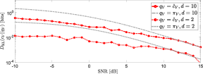
Figure 1: Approximation quality of $c_{V}$. Comparison between CODINE method $\hat{c}_{V}$ and the flat copula density $\pi_{V}$ for different values of the signal-to-noise ratio (SNR) and for different dimensionality $d$ of the input.

To assess the quality of the copula density estimator $\hat{c}_{U}(\mathbf{u})$, we propose the following set of self-consistency tests over the basic property illustrated in (13). In particular,

1. if $\hat{c}_{U}(\mathbf{u})$ is a well-defined density and $\hat{c}_{U}(\mathbf{u})=c_{U}(\mathbf{u})$, then the following relation must hold

   $$\mathbb{E}_{\mathbf{u}\sim\pi_{U}(\mathbf{u})}\bigl{[}\hat{c}_{U}(\mathbf{u})\bigr{]}=1,$$ (14)

2. in general, for any $n$-th order moment, if $\hat{c}_{U}(\mathbf{u})$ is a well-defined density and $\hat{c}_{U}(\mathbf{u})=c_{U}(\mathbf{u})$, then

   $$\mathbb{E}_{\mathbf{u}\sim\pi_{U}(\mathbf{u})}\bigl{[}U^{n}\cdot\hat{c}_{U}(\mathbf{u})\bigr{]}=\mathbb{E}_{\mathbf{u}\sim c_{U}(\mathbf{u})}\bigl{[}U^{n}\bigr{]}.$$ (15)

The first test verifies that the copula density integrates to one while the second set of tests extends the first test to the moments of any order. Similarly, joint consistency tests can be defined, e.g., the Spearman rank correlation $\rho_{X,Y}$ between pairs of variables can be rewritten in terms of their joint copula density $\hat{c}_{UV}$ and it reads as follows

$$\rho_{X,Y}=12\cdot\mathbb{E}_{(\mathbf{u},\mathbf{v})\sim\pi_{U}(\mathbf{u})\pi_{V}(\mathbf{v})}\bigl{[}UV\cdot\hat{c}_{UV}(\mathbf{u},\mathbf{v})\bigr{]}-3.$$ (16)

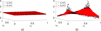
Figure 2: Ground-truth and estimated copula density (SNR=$0$ dB) at the channel output ($d=2$) using the GAN $f$ generator for: a) uncorrelated noise $\rho=0$. b) correlated noise with coefficient $\rho=0.5$.

When the copula density is known, it is possible to assess the quality of the copula density neural estimator $\hat{c}_{U}(\mathbf{u})$ by computing the Kullback-Leibler (KL) divergence between the true and the estimated copulas

$$Q_{c}=D_{\text{KL}}(c_{U}||\hat{c}_{U})=\mathbb{E}_{\mathbf{u}\sim c_{U}(\mathbf{u})}\biggl{[}\log\frac{c_{U}(\mathbf{u})}{\hat{c}_{U}(\mathbf{u})}\biggr{]}.$$ (17)

Once the dependence structure is characterized via a valid copula density $\hat{c}_{U}(\mathbf{u})$, a multiplication with the estimated marginal components $\hat{p}_{X_{i}}(x_{i})$, $\forall i=\{1,\dots,d\}$ yields the estimate of the joint pdf $\hat{p}_{X}(\mathbf{x})$. In general, it is rather simple to build one-dimensional marginal density estimates $\hat{p}_{X_{i}}(x_{i})$, e.g., using histograms or kernel functions.

Now, as a first example to validate the density estimator, we consider the transmission of $d$-dimensional Gaussian samples over an additive white Gaussian channel (AWGN). Given the AWGN model $Y=X+N$, where $X\sim\mathcal{N}(0,\mathbb{I})$ and $N\sim\mathcal{N}(0,\Sigma_{N})$, it is simple to obtain closed-form expressions for the probability densities involved. In particular, the copula density of the output $Y$ reads as in (12), where $\mathbf{F}_{X}(\mathbf{x})$ is an operator that element-wise applies transform sampling (via Gaussian cumulative distributions) to the components of $\mathbf{x}$ such that $(\mathbf{u},\mathbf{v})=(\mathbf{F}_{X}(\mathbf{x}),\mathbf{F}_{Y}(\mathbf{y}))$ and $\tilde{\Sigma}_{N}=\Sigma_{N}\odot\mathbb{I}$, where $A\odot B$ denotes the Hadamard product between $A$ and $B$.

In Fig.1 we illustrate the KL divergence (in bits) between the ground-truth and the neural estimator obtained using the $f$-GAN generator reported in Tab.I. To work with non-uniform copula structures, we study the case of non-diagonal noise covariance matrix $\Sigma_{N}$. In particular, we impose a tridiagonal covariance matrix such that $\Sigma_{N}=\sigma_{N}^{2}R$ where $R_{i,i}=1$ with $i=1,\dots,d$, and $R_{i,i+1}=\rho$, with $i=1,\dots,d-1$ and $\rho=0.5$. Moreover, Fig.1 also depicts the quality of the approximation for different values of the signal-to-noise ratio (SNR), defined as the reciprocal of the noise power $\sigma_{N}^{2}$, and for different dimensions $d$. To provide a numerical comparison, we also report the KL divergence $D_{\text{KL}}(c_{V}||\pi_{V})$ between the ground-truth and the flat copula density $\pi_{V}=1$. It can be shown that when $c_{V}$ is Gaussian, we obtain

$$D_{\text{KL}}(c_{V}||\pi_{V})=\frac{1}{2}\log\biggl{(}\frac{\det(\tilde{\Sigma}_{N}+\mathbb{I})}{\det(\Sigma_{N}+\mathbb{I})}\biggr{)}.$$ (18)

Notice that in Fig.1 we use the same simple neural network architecture for both $d=2$ and $d=10$. Nonetheless, CODINE can accurately approximate multidimensional densities even without any further hyper-parameter search. Fig.2a reports a comparison between ground-truth and estimated copula densities at $0$ dB in the case of independent components ($\rho=0$) and correlated components ($\rho=0.5$). It is worth mentioning that when there is independence between components, the copula density is everywhere unitary $c_{V}(\mathbf{v})$$=$$1$. Hence, independence tests can be derived based on the structure of the estimated copula via CODINE, but we leave it for future discussions.

V Applications

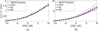
Figure 3: Estimated mutual information $I(X;Y)$ via joint copula $c_{UV}$ with different generators $f$ for: a) $d=1$. b) $d=5$.

V-A Mutual Information Estimation

Given two random variables, $X$ and $Y$, the mutual information $I(X;Y)$ quantifies the statistical dependence between $X$ and $Y$. It measures the amount of information obtained about one variable via the observation of the other and it can be rewritten also in terms of KL divergence as ${I}(X;Y)=D_{\text{KL}}(p_{XY}||p_{X}p_{Y})$. From Sklar’s theorem, it is simple to show that the mutual information can be computed using only copula densities as follows

$${I}(X;Y)=\mathbb{E}_{(\mathbf{u},\mathbf{v})\sim c_{UV}(\mathbf{u},\mathbf{v})}\biggl{[}\log\frac{c_{UV}(\mathbf{u},\mathbf{v})}{c_{U}(\mathbf{u})c_{V}(\mathbf{v})}\biggr{]}.$$ (19)

Therefore, (19) requires three separate copula densities estimators, each of which obtained as explained in Section III. Alternatively, one could learn the copulas density ratio via maximization of the variational lower bound on the mutual information. Using again Fenchel duality, the KL divergence

$$\small D_{\text{KL}}(c_{UV}||c_{U}c_{V})=\int_{[0,1]^{2d}}{c_{UV}(\mathbf{u},\mathbf{v})\log\biggl{(}\frac{c_{UV}(\mathbf{u},\mathbf{v})}{c_{U}(\mathbf{u})c_{V}(\mathbf{v})}\biggr{)}\mathop{}\!\mathrm{d}\mathbf{u}\mathop{}\!\mathrm{d}\mathbf{v}}$$ (20)

corresponds to the supremum over $T$ of

$$\small\mathcal{J}_{\text{KL}}(T)=\mathbb{E}_{c_{UV}}\biggl{[}T\bigl{(}\mathbf{u},\mathbf{v}\bigr{)}\biggr{]}-\mathbb{E}_{c_{U}c_{V}}\biggl{[}\exp{\bigl{(}T\bigl{(}\mathbf{u},\mathbf{v}\bigr{)}-1\bigr{)}}\biggr{]}.$$ (21)

When $X$ is a univariate random variable, its copula density $c_{U}$ is unitary. Notice that (21) can be seen as a special case of the more general (5) when $f$ is the generator of the KL divergence and the second expectation is not done over independent uniforms with distribution $\pi_{U}$ but over samples from the product of copula densities $c_{U}\cdot c_{V}$. We estimate the mutual information between $X$ and $Y$ in the AWGN model using the generators described in Tab.I. Fig.3a and Fig.3b show the estimated mutual information for $d=1$ and $d=5$, respectively, and compare it with the closed-form capacity formula $I(X;Y)=d/2\log_{2}(1+\text{SNR})$.

V-B Data Generation

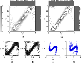
Figure 4: Toy example contour plot and marginal densities of a) ground-truth copula density $c_{u}$ obtained using kernel density estimation and b) copula density neural estimate $\hat{c}_{u}$. c) Pseudo-observations. d) Data generated in the uniform probability space via Gibbs sampling. e) Observations. f) Data generated in the sample domain via inverse transform sampling.

As a second application example, we generate $n$ new pseudo-observations $\{\hat{\mathbf{u}}^{(1)},\dots,\hat{\mathbf{u}}^{(n)}\}$ from $\hat{c}_{U}$ by deploying a Markov chain Monte Carlo (MCMC) algorithm. Validating the quality of the generated data provides an alternative path for assessing the copula estimate itself. We propose to use Gibbs sampling to extract valid uniform realizations of the copula estimate. In particular, we start with an initial guess $\hat{\mathbf{u}}^{(0)}$ and produce next samples $\hat{\mathbf{u}}^{(i+1)}$ by sampling each component from univariate conditional densities $\hat{c}_{U}(u_{j}^{(i+1)}|u_{1}^{(i+1)},\dots,u_{j-1}^{(i+1)},u_{j+1}^{(i)},\dots,u_{d}^{(i)})$ for $j=1,\dots,d$. It is clear that the generated data in the sample domain is obtained via inverse transform sampling through the estimated quantile functions $\hat{F}_{X_{i}}^{-1}$.

Consider a bi-dimensional random variable whose realizations have form $\mathbf{x}=[\mathbf{x}_{1},\mathbf{x}_{2}]$ and for which we want to generate new samples $\mathbf{\hat{x}}=[\mathbf{\hat{x}}_{1},\mathbf{\hat{x}}_{2}]$. To force a non-linear statistical dependence structure, we define a toy example $\mathbf{x}$ as $\mathbf{x}=[\sin(t),t\cos(t)]+\mathbf{n}$, where $t\sim\mathcal{N}(0,1)$ and $\mathbf{n}\sim\mathcal{N}(\mathbf{0},\sigma^{2}\mathbb{I})$ with $\sigma=0.1$. We use CODINE to estimate its copula density and sample from it via Gibbs sampling. Fig.4 compares the copula density estimate obtained via kernel density estimation (Fig.4a) with the estimate obtained using CODINE (Fig.4b). It also shows the generated samples in the uniform (Fig.4d) and in the sample domain (Fig.4f). Lastly, the difference between $\mathbf{x}$ and $\hat{\mathbf{x}}$ are mainly due to Gibbs sampling mechanism as it can be observed from Fig.4d and Fig.4f.

VI Conclusions

This paper presented CODINE, a copula density neural estimator. It works by maximizing a variational lower bound on the $f$-divergence between two distributions defined on the uniform probability space, namely, the distribution of the pseudo-observations and the distribution of independent uniforms. CODINE also provides alternative approaches for measuring statistical dependence, mutual information, and for data generation.

References

- [1] B. W. Silverman, Density Estimation for Statistics and Data Analysis. London: Chapman & Hall, 1986.
- [2] A. Van Den Oord, N. Kalchbrenner, and K. Kavukcuoglu, “Pixel recurrent neural networks,” in International Conference on Machine Learning, 2016, p. 1747–1756.
- [3] L. Dinh, J. Sohl-Dickstein, and S. Bengio, “Density estimation using real NVP,” in International Conference on Learning Representations, 2017.
- [4] I. Goodfellow, J. Pouget-Abadie, M. Mirza, B. Xu, D. Warde-Farley, S. Ozair, A. Courville, and Y. Bengio, “Generative adversarial nets,” in Advances in Neural Information Processing Systems, vol. 27, 2014.
- [5] D. P. Kingma and M. Welling, “Auto-encoding variational bayes,” in 2nd International Conference on Learning Representations, ICLR 2014, Banff, AB, Canada, April 14-16, 2014, 2014.
- [6] J. Ho, A. Jain, and P. Abbeel, “Denoising diffusion probabilistic models,” in Advances in Neural Information Processing Systems, vol. 33, 2020, pp. 6840–6851.
- [7] N. A. Letizia and A. M. Tonello, “Segmented generative networks: Data generation in the uniform probability space,” IEEE Transactions on Neural Networks and Learning Systems, pp. 1–10, 2020.
- [8] R. B. Nelsen, An Introduction to Copulas. Berlin, Heidelberg: Springer-Verlag, 2006.
- [9] A. Sklar, “Fonctions de répartition à n dimensions et leurs marges,” Publications de l’Institut de Statistique de l’Université de Paris, vol. 8, pp. 229–231, 1959.
- [10] S. Demarta and A. J.McNeil, “The t copula and related copulas,” International Statistical Review, vol. 73, no. 1, pp. 111–129, 4 2005.
- [11] C. Czado and T. Nagler, “Vine copula based modeling,” Annual Review of Statistics and Its Application, vol. 9, 03 2022.
- [12] X. Nguyen, M. J. Wainwright, and M. I. Jordan, “Estimating divergence functionals and the likelihood ratio by convex risk minimization,” IEEE Transactions on Information Theory, vol. 56, no. 11, pp. 5847–5861, 2010.
- [13] N. A. Letizia and A. M. Tonello, “CODINE copula density neural estimator,” https://github.com/tonellolab/CODINE-copula-estimator, 2022.
- [14] B. Poczos, Z. Ghahramani, and J. Schneider, “Copula-based kernel dependency measures,” Proceedings of the 29th International Conference on Machine Learning, ICML 2012, vol. 1, 06 2012.
- [15] G. Papamakarios and I. Murray, “Distilling intractable generative models,” in Probabilistic Integration Workshop at the Neural Information Processing Systems Conference, 2015, Aug. 2015.
- [16] D. Rezende and S. Mohamed, “Variational inference with normalizing flows,” in Proceedings of the 32nd International Conference on Machine Learning, vol. 37. Lille, France: PMLR, 07–09 Jul 2015, pp. 1530–1538.