RankDNN: Learning to Rank for Few-shot Learning

Abstract

This paper introduces a new few-shot learning pipeline that casts relevance ranking for image retrieval as binary ranking relation classification. In comparison to image classification, ranking relation classification is sample efficient and domain agnostic. Besides, it provides a new perspective on few-shot learning and is complementary to state-of-the-art methods. The core component of our deep neural network is a simple MLP, which takes as input an image triplet encoded as the difference between two vector-Kronecker products, and outputs a binary relevance ranking order. The proposed RankMLP can be built on top of any state-of-the-art feature extractors, and our entire deep neural network is called the ranking deep neural network, or RankDNN. Meanwhile, RankDNN can be flexibly fused with other post-processing methods. During the meta test, RankDNN ranks support images according to their similarity with the query samples, and each query sample is assigned the class label of its nearest neighbor. Experiments demonstrate that RankDNN can effectively improve the performance of its baselines based on a variety of backbones and it outperforms previous state-of-the-art algorithms on multiple few-shot learning benchmarks, including miniImageNet, tieredImageNet, Caltech-UCSD Birds, and CIFAR-FS. Furthermore, experiments on the cross-domain challenge demonstrate the superior transferability of RankDNN.The code is available at: https://github.com/guoqianyu-alberta/RankDNN.

Introduction

Contrary to the normal practice of using a large amount of labeled data (krizhevsky2012imagenet; He et al. 2016), few-shot learning (Lu et al. 2020; Afrasiyabi, Lalonde, and Gagne 2021) refers to learning new concepts from a very small amount of data by leveraging the learning “skills” gained from many similar learning tasks. State-of-the-art methods (Ma et al. 2021; Hong et al. 2021; Tang et al. 2021; Rizve et al. 2021) attempt to learn meta knowledge that can be transferred to new tasks. Although much progress has been made, recently proposed methods still bear the risk of unsatisfactory generalization performance on new tasks. The reason is two-fold. First, the meta knowledge they learn may have limited transferability and may not be well applicable to certain new tasks. Second, there is simply too little data available for new tasks and overfitting is very hard to avoid. Modern deep neural networks are so flexible and overparameterized that they can even perfectly fit image data with random labels, as stated in (Zhang et al. 2021; Arpit et al. 2017). Overfitting creates a large gap between training and testing performance.

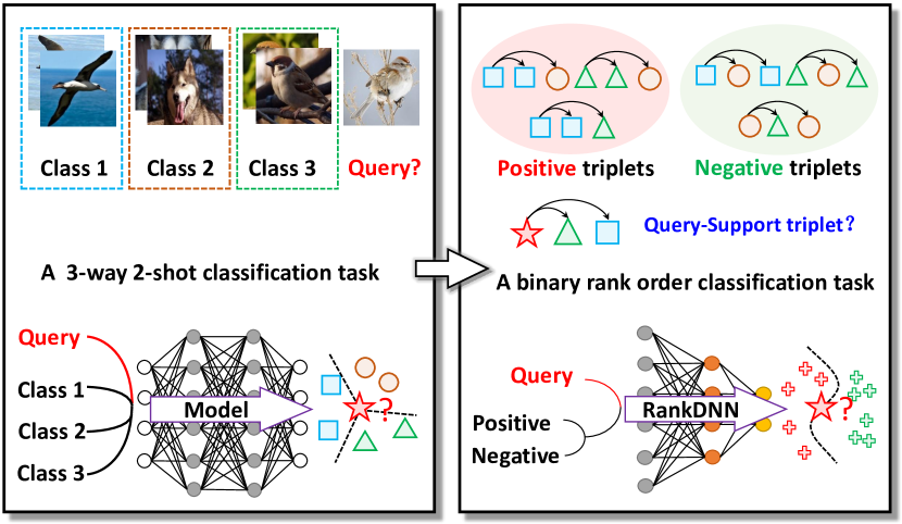
Figure 1: Ranking deep neural network (RankDNN) establishes a learning framework that can cast a $N$-way-$K$-shot learning task into a binary relevance ranking problem, which is sample efficient and domain agnostic.

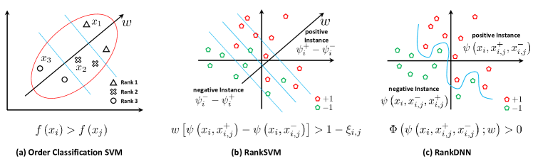
Figure 2: Comparison of ranking learning frameworks. (a) Pointwise ranking algorithms, such as McRank (Li, Wu, and Burges 2007; Shashua, Levin et al. 2003) and OC SVM, cast the ranking learning problem as a regression or classification task on single objects. (b) Pairwise ranking algorithms, such as RankSVM (Joachims 2002; Prosser et al. 2010), models binary relevance ranking within object pairs. (c) The proposed RankDNN generalizes binary relevance ranking in RankSVM into binary triplet classification with deep neural networks.

Inspired by relevance ranking in information retrieval (Shashua, Levin et al. 2003; Joachims 2002), we consider binary relevance ranking for few-shot learning, as shown in Fig 1. Given a query image and two support images in a given order, binary relevance ranking ranks the relevance of these support images concerning the query image. There are only two possible outcomes of this ranking problem. That is, the first support image is more relevant than the second one or vice versa. Relevance ranking among images focuses on the similarity of images, especially the similarity of foreground objects, but not the specific categories of images or foreground objects. Thus a relevance ranking model should be able to grasp the meta knowledge about the assessment of image or object similarity regardless of their specific contents. Such a capability endows the learned model a strong transferability to a wide range of new tasks where specific image contents may vary. Meanwhile, as we need three images for each binary relevance ranking instance, the number of training samples for ranking is greatly expanded by constructing triplets, which significantly alleviates training data shortage in few-shot learning.

We develop a ranking learning framework for few-shot image classification, which is formulated as a query-support relevance ranking problem. We generalize the SVM based ranking learning idea in OC SVM (Shashua, Levin et al. 2003) and RankSVM (Joachims 2002) to deep neural networks, and call the proposed framework RankDNN. Meanwhile, we provide a new perspective on image classification by converting a multiclass classification task into a binary classification task.

To implement binary relevance ranking of two support images to a query image, there are two key issues: The first issue is how to simultaneously encode the semantic features of an image triplet as well as the roles and order of the three images in the triplet; the second issue is which machine learning algorithm should be used to produce the binary ranking result. Encoding an image triplet while preserving all necessary information is very challenging. We use the query image in the triplet to form two query-support pairs with the two support images, and encode each query-support pair using the outer product, also called vector-Kronecker product, of their feature vectors. The entire image triplet is finally represented using the difference between these two vector outer products. Our intuition behind this encoding scheme is that the vector-Kronecker product of two feature vectors can not only preserve all information in the original feature vectors but also model the correlation between any two dimensions of these features. In addition, the sign of the final difference encodes the order of the two support images in the triplet.

In summary, this paper has the following contributions:

$\bullet$

We introduce a new ranking learning framework for few-shot learning called ranking deep neural network (or RankDNN), which decomposes a few-shot image classification task into multiple binary relevance ranking problems. By constructing image triplets for such binary ranking problems, our framework generates a large amount of training data across different image classes.

$\bullet$

We propose a novel image triplet encoding scheme based on vector-Kronecker products. It preserves all necessary information in an image triplet and can also model the correlation between any two feature dimensions respectively of the query image and one of the support images.

$\bullet$

Experiments demonstrate that our RankDNN outperforms its baselines in many different scenarios and achieves state-of-the-art performance on multiple few-shot learning benchmarks , including miniImageNet,  (Vinyals et al. 2016), tieredImageNet,  (ren2018meta), Caltech-UCSD Birds (Wah et al. 2011), and CIFAR-FS. (Bertinetto et al. 2018). Besides, the fusion experiments, cross-domain challenges and different backbones experiments prove the generalization, flexibility and robustness of RankDNN.

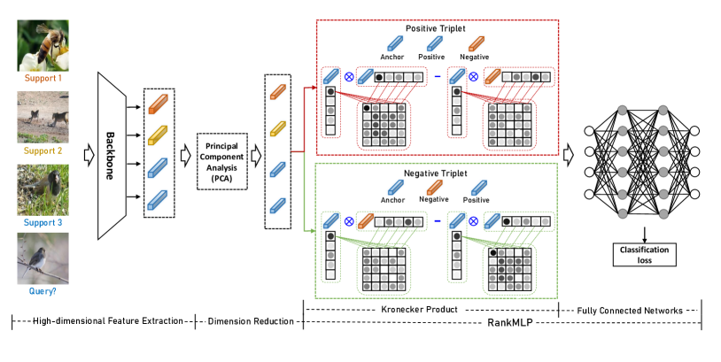
Figure 3: The ranking deep neural network is composed of a high-dimensional feature extractor, a dimension reduction part and a ranking multilayer preceptron. The parameters feature extractor are frozen all the time and the RankMLP are trained consecutively in different stages.

Related Work

Few-shot Learning. Few-shot learning aims to recognize samples from unseen classes with limited training data, which is expect to reduce labeling cost, achieve a low-cost and quick model deployment. Various few-shot learning algorithms have been proposed, such as Matching Net (Vinyals et al. 2016), Relation Net (Sung et al. 2018), MAML (Finn, Abbeel, and Levine 2017), and TAML (Jamal and Qi 2019). However, according to (Chen et al. 2019a; Gidaris and Komodakis 2018; Qiao et al. 2018), since there are two few annotated samples, state-of-the-art algorithms (Mangla et al. 2020; Rizve et al. 2021) focus on solving the over-fitting problem by self-supervised learning. There are also many other methods that try to learn meta knowledge with the strong generalization ability (Hong et al. 2021; Tang et al. 2021).In this paper, we provide a new perspective to solve the few-shot learning problem by converting it into a relevance ranking task. Then our learning task is built upon image triplets and becomes domain agnostic. Since there are a large amount of triplet combinations even with few samples, the overfitting problem can be alleviated greatly.

Learning to Rank. Applying existing and effective machine learning methods to rank is called learning to rank, such as RankSVM(Joachims 2002) and RankNet(Burges et al. 2005). Learning to rank is not only widely used in major tasks of natural language processing(Masuda 2003; Briakou and Carpuat 2020; Zhang and van Genabith 2020), but also has attracted the attention of metric learning in recent years(Liu et al. 2021; Cakir et al. 2019; Wang et al. 2019a). (Wang et al. 2019a) proposed ranked-based list loss with structured information of multiple samples to improve the training efficiency of metric learning. Although DeepRank (Pang et al. 2017) utilizes deep neural networks to conduct similarity ranking, its learning objective is a pairwise contrastive loss which is widely used in metric learning. While in RankDNN, we convert the rank problem into a binary classification problem and solve it with gradient-based methods. Meanwhile, compared with that in (Prosser et al. 2010), we propose a much more efficient triplet feature the construction method for few-shot learning and solve it with deep neural network flexibly.

A Ranking Learning Framework for Few-shot Image Classification

The general regime of an N-way K-shot classification task $\mathcal{T}$: with $N$ previously unseen image categories, each of which contains $K$ samples, the task aims to build a classifier to classify a set of query images into these $N$ categories. The dataset for task $\mathcal{T}$ is $\mathcal{D}_{\mathcal{T}}=\mathcal{S}\cup\mathcal{Q}$ where $\mathcal{S}=\left\{\left(\boldsymbol{x}_{i},y_{i}\right)\right\}_{i=1}^{N\times K}$ is the support set, $\mathcal{Q}=\left\{\left(\boldsymbol{x}_{i},y_{i}\right)\right\}_{i=N\times K+1}^{N\times K+T}$ is the query set, $T$ is the number of query samples. $\boldsymbol{x}_{i}$ and $y_{i}(\in\left\{C_{1},...,C_{N}\right\}=\mathcal{C}_{\mathcal{T}}\subset\mathcal{C}$) are respectively the $i$-the image sample and its label. State-of-the-art methods often formalize few-shot image classification as a metric learning (Zhang et al. 2020a; Mangla et al. 2020) or multiclass classification task (Rizve et al. 2021; Chen et al. 2021a; Yang, Liu, and Xu 2021). However, in this paper, we cast few-shot classification as an image retrieval task. Given a query image $\boldsymbol{x}_{q}$ and a support image collection $\mathcal{S}$, a retrieval system should return a complete ranked list $r^{*}(\boldsymbol{x}_{q})$, that sorts the support images in $\mathcal{S}$ according to their relevance to the query as follows.

$$r^{*}(\boldsymbol{x}_{q}):\boldsymbol{x}_{q_{1}}\succ\boldsymbol{x}_{q_{2}}\succ\cdots\succ\boldsymbol{x}_{q_{N\times K}},$$ (1)

where $\boldsymbol{x}_{q_{k}}\in\mathcal{S}$, and $\boldsymbol{x}_{q_{i}}\succ\boldsymbol{x}_{q_{j}}$ means $\boldsymbol{x}_{q_{i}}$ is more relevant to $\boldsymbol{x}_{q}$ than $\boldsymbol{x}_{q_{j}}$. The formula in (1) indicates how an image retrieval system works (Ge 2018; Wang et al. 2020; Levi et al. 2021). Most metric learning based methods (Zhang et al. 2020a; Snell, Swersky, and Zemel 2017) for few-shot learning aim to find a unified embedding space where every query sample is assigned the class label of its nearest support image.

Inspired by the approach in (Joachims 2002; Prosser et al. 2010), we decompose the complete relevance ranking relation among multiple variables into several binary relevance ranking relations over $\mathcal{S}\times\mathcal{S}$. Thus, we have

$$\forall\left(\boldsymbol{x}_{q_{i}},\boldsymbol{x}_{q_{j}}\right)\in r^{*}\left(\boldsymbol{x}_{q}\right)(i<j):\boldsymbol{x}_{q_{i}}\succ\boldsymbol{x}_{q_{j}},\boldsymbol{x}_{q_{j}}\prec\boldsymbol{x}_{q_{i}}.$$ (2)

There are $\mathcal{O}\left(\left|\mathcal{S}\right|^{2}\right)$ such relevance ranking pairs. The following 5-way-1-shot task is given as an example:

$${\color[rgb]{1,0,0}\boldsymbol{x}_{q_{1}}\succ\boldsymbol{x}_{q_{2}}},{\color[rgb]{1,0,0}\boldsymbol{x}_{q_{1}}\succ\boldsymbol{x}_{q_{3}}},{\color[rgb]{1,0,0}\boldsymbol{x}_{q_{1}}\succ\boldsymbol{x}_{q_{4}}},{\color[rgb]{1,0,0}\boldsymbol{x}_{q_{1}}\succ\boldsymbol{x}_{q_{5}}};$$ (3)

$${\color[rgb]{0,0,1}\boldsymbol{x}_{q_{2}}\prec\boldsymbol{x}_{q_{1}}},{\color[rgb]{1,0,0}\boldsymbol{x}_{q_{2}}\succ\boldsymbol{x}_{q_{3}}},{\color[rgb]{1,0,0}\boldsymbol{x}_{q_{2}}\succ\boldsymbol{x}_{q_{4}}},{\color[rgb]{1,0,0}\boldsymbol{x}_{q_{2}}\succ\boldsymbol{x}_{q_{5}}};$$

$${\color[rgb]{0,0,1}\boldsymbol{x}_{q_{3}}\prec\boldsymbol{x}_{q_{1}}},{\color[rgb]{0,0,1}\boldsymbol{x}_{q_{3}}\prec\boldsymbol{x}_{q_{2}}},{\color[rgb]{1,0,0}\boldsymbol{x}_{q_{3}}\succ\boldsymbol{x}_{q_{4}}},{\color[rgb]{1,0,0}\boldsymbol{x}_{q_{2}}\succ\boldsymbol{x}_{q_{5}}};$$

$${\color[rgb]{0,0,1}\boldsymbol{x}_{q_{4}}\prec\boldsymbol{x}_{q_{1}}},{\color[rgb]{0,0,1}\boldsymbol{x}_{q_{4}}\prec\boldsymbol{x}_{q_{2}}},{\color[rgb]{0,0,1}\boldsymbol{x}_{q_{4}}\prec\boldsymbol{x}_{q_{3}}},{\color[rgb]{1,0,0}\boldsymbol{x}_{q_{4}}\succ\boldsymbol{x}_{q_{5}}};$$

$${\color[rgb]{0,0,1}\boldsymbol{x}_{q_{5}}\prec\boldsymbol{x}_{q_{1}}},{\color[rgb]{0,0,1}\boldsymbol{x}_{q_{5}}\prec\boldsymbol{x}_{q_{2}}},{\color[rgb]{0,0,1}\boldsymbol{x}_{q_{5}}\prec\boldsymbol{x}_{q_{3}}},{\color[rgb]{0,0,1}\boldsymbol{x}_{q_{5}}\prec\boldsymbol{x}_{q_{4}}}.$$

The query image $\boldsymbol{x}_{q}$ is then assigned the class label of the support sample ranked first. By exploiting such binary relations, we can obtain an extensive number of training samples in few-shot learning, avoid the necessity to obtain a complete ranked list, and tolerate minor inconsistencies in binary ranking results.

According to Eq. (2), we need to formulate the binary relevance ranking relation between any two support images $(\boldsymbol{x}_{i},\boldsymbol{x}_{j})$ for a query sample $\boldsymbol{x}_{q}$. There are two key elements in describing such a relation: First, an informative encoding scheme $\psi\left(\cdot;\theta\right)$ ($\theta$ denotes the parameters of $\psi$) to encode the semantic features as well as the detailed component-wise correlations between a query image and a support image; second, a scoring function $\Phi$ to evaluate the overall similarity or relevance between a query image and a support image. Then a binary relevance ranking relation can be concretely formulated as follows:

$$\boldsymbol{x}_{i}\succ_{r^{*}(q)}\boldsymbol{x}_{j}\iff\Phi\left(\psi\left(x_{q},x_{i}\right);w\right)>\Phi\left(\psi\left(x_{q},x_{j}\right);w\right),$$ (4)

where $w$ denotes the learnable parameters of the scoring function. RankSVM (Joachims 2002) adopts the class of linear scoring functions, and the binary ranking learning problem becomes finding the weight vector that fulfills the most inequalities in Eq. 2, which can be formulated as follows.

$$\min\limits_{w,\vec{\xi}}\frac{1}{2}\left\|w\right\|^{2}+C\sum\limits_{i,j,k}\xi_{i,j,k}$$

s.t. $$\forall\boldsymbol{x}_{i}\succ_{r^{*}\left(q\right)}\boldsymbol{x}_{j}:w\left[\psi\left(x_{q},x_{i}\right)-\psi\left(x_{q},x_{j}\right)\right]>1-\xi_{i,j,q}$$ (5)

$$\forall i\forall j\forall q:\xi_{i,j,q}>0,$$

where $C$ is a constant, $\xi_{i,j,q}$ is a slack variable. RankSVM (Joachims 2002) can be extended to use non-linear scoring functions via kernel methods.

In Fig 2, the few-shot classification problem can now be cast as a binary classification task and solved by RankSVM. To step further, we wish to obtain a more general formulation about the ranking learning problem. Given a query sample $x_{q}$, there are two kinds of ranking relations: if $\Phi\left(\psi\left(x_{q},x_{i}\right);w\right)>\Phi\left(\psi\left(x_{q},x_{j}\right);w\right)$, $\left\langle x_{q},x_{i},x_{j}\right\rangle$ is identified as a positive triplet sample; otherwise, $\Phi\left(\psi\left(x_{q},x_{i}\right);w\right)\leq\Phi\left(\psi\left(x_{q},x_{j}\right);w\right)$, and $\left\langle x_{q},x_{i},x_{j}\right\rangle$ is a negative triplet sample. Then we can define a unified triplet encoding scheme, which not only encodes the feature vectors of the query and support samples in the triplet, but also their roles and order in the triplet as well as their interactions. In a training triplet, one of the support samples should come from the same class as the query sample while the other support sample should come from a different class. We can automatically generate the ground-truth binary class label of a triplet as follows,

$$y\left(\left\langle x_{q},x_{i},x_{j}\right\rangle\right)=\{\begin{matrix}+1,\textup{if}~{}~{}{x}_{i}\succ_{r^{*}\left(q\right)}{x}_{j};\\ -1,\textup{if}~{}~{}{x}_{i}\prec_{r^{*}\left(q\right)}{x}_{j}.\end{matrix}$$ (6)

In this paper, we generalize the linear/nonlinear scoring function $\Phi$ in RankSVM to an MLP based binary classifier, called RankMLP. RankMLP is trained using the following overall loss function,

$$\mathcal{L}_{rank}=\frac{1}{N_{t}}\sum\limits_{q,i,j}\mathcal{L}_{bce}\left(\Phi\left(\psi\left(\left\langle x_{q},x_{i},x_{j}\right\rangle;\theta\right);w\right),y_{q,i,j}\right),$$ (7)

where $N_{t}$ is the number of triplets in a mini-batch, $\mathcal{L}_{bce}$ is the binary cross-entropy loss, and $y_{q,i,j}$ is the ground-truth binary class label of a triplet.

Discussion. According to Eqs. (6) and (7), we solve the ranking learning problems with deep neural networks, as in information retrieval (Palangi et al. 2016; Pang et al. 2017) and metric learning (Cakir et al. 2019; Liu et al. 2021). The main difference is that RankMLP focuses on binary ranking relation classification but not the distance constraints in metric learning. Given an $N$-way-$K$-shot task in the training set of a few-shot learning problem, we can construct $(N-1)K(K-1)$ training triplets for every query sample, which significantly alleviates the data shortage.

The Ranking Deep Neural Network

Overview

The ranking deep neural network (RankDNN) takes in an image triplet and outputs whether this triplet is a positive sample or a negative sample. Although some existing deep metric learning methods (Cakir et al. 2019; Liu et al. 2021) already use the ranking loss, a key difference here is that inter-class variations are much more challenging in few-shot learning than those in image retrieval. In our experiments, directly training a deep neural network from end to end to classify triplets would lead to gradient explosion. In Fig 3, the RankDNN pipeline contains two parts: a frozen high-dimensional feature extractor $f\left(\cdot,\boldsymbol{\theta}_{e}\right)$ and a ranking deep neural network $\Phi\left(\cdot,\boldsymbol{\theta}\right)$.

Algorithm 1 outlines the training phase of RankDNN for few-shot learning. Given an image triplet $\left\langle x_{q},x_{i},x_{j}\right\rangle$, RankDNN uses state-of-the-art feature extractors, such as S2M2 (Mangla et al. 2020) and IE (Rizve et al. 2021), to extract discriminative features $f\left(x_{q};\boldsymbol{\theta}_{e}\right),f\left(x_{i};\boldsymbol{\theta}_{e}\right),f\left(x_{j};\boldsymbol{\theta}_{e}\right)\in\mathbb{R}^{640}$. For simplicity, we write $f\left(x_{q};\boldsymbol{\theta}_{e}\right)$ as $f_{q}$. To generate subsequent features for triplet classification, we use PCA (Yang et al. 2004) to reduce the image feature dimension from 640 to 80. During the training stage, we freeze both the feature extractor and the PCA transform, and train RankMLP with the loss function $\mathcal{L}_{rank}$ defined in Eq. (7).

Input: Training data $\mathcal{D}=\left\{\left(\boldsymbol{x}_{i},y_{i}\right)\right\}_{k=1}^{N}$. Network $f\left(\cdot,\boldsymbol{\theta}_{e}\right)$ initialized with a state-of-the-art pretrained model. The ranking neural network $\Phi\left(\cdot,\boldsymbol{\theta}\right)$ initialized with randomly noises.

Output: The learnable parameters $\boldsymbol{\theta}$ of the neural networks $\Phi\left(\cdot,\boldsymbol{\theta}\right)$.

1 // conduct PCA transform for the dimension reduction

2 Extract features of all training images and learn a principal component analysis transform (PCA) $T$;

3 // train the ranking neural network $\Phi$ and freeze the feature extractor $f_{e}$ all the time

4 while not converge do

5       $t\leftarrow t+1$;

6       Sample anchors randomly and their neighborhoods according to the method in HTL (Ge 2018);

7       Extract features with $f_{e}\left(\cdot,\boldsymbol{\theta}_{e}\right)$, and freeze it;

8       Reduce the feature dimension with PCA;

9       Construct the triplet ranking description with Eq. 9 and pass it through the RankMLP $\Phi\left(\cdot,\boldsymbol{\theta}\right)$;

10       Compute the binary cross entropy loss in a mini-batch $\mathcal{L}_{rank}$ with Eq. 7;

11       Backpropagate the gradients produced at the loss layer and update the learnable parameters $\boldsymbol{\theta}$.

12 end while

Algorithm 1 Meta-Training of RankDNN for Few-shot Learning

Triplet Encoding Scheme

Encoding triplets of extracted features plays a precursory role for RankMLP. The Kronecker product is a matrix algebra operation that produces structured descriptions for modeling complex systems. If $A\in\mathbb{R}^{n_{a}\times m_{a}}$ and $B\in\mathbb{R}^{n_{a}\times m_{a}}$, their Kronecker product is denoted by $A\otimes B$ and defined as follows:

$$A\otimes B\equiv{\begin{bmatrix}{a_{11}\bf{B}}&\cdots&{a_{1n}\bf{B}}\\ \vdots&\ddots&\vdots\\ {a_{n1}\bf{B}}&\cdots&{a_{nn}\bf{B}}\end{bmatrix}}.$$

When both matrices degenerate to vectors $x\in{\mathbb{R}^{d\times{1}}}$ and $y\in{\mathbb{R}^{1\ times{d}}}$, their Kronecker product is actually the same as their outer product; and is called vector-Kronecker product in this paper. It is formulated in the following equation:

$$\bf{x}\otimes\bf{y}\equiv{\begin{bmatrix}{x_{1}y_{1}}&\cdots&{x_{1}y_{n}}\\ \vdots&\ddots&\vdots\\ {x_{n}y_{1}}&\cdots&{x_{n}y_{n}}\end{bmatrix}}.$$ (8)

In the literature (De Launey and Seberry 1994; Langville and Stewart 2004; Broxson 2006), the Kronecker product of graphs is one of the usual names of the categorical product of graphs, also called the tensor product. This product of graphs was studied by various authors (Azevedo et al. 2020; Weichsel 1962; Mamut and Vumar 2008), who proved that Kronecker product can encode the connectivity and relationship between graphs.

Given a triplet of feature descriptors $\left\langle f_{q},f_{i},f_{j}\right\rangle$, state-of-the-art methods (Chen et al. 2021a; Rizve et al. 2021) calculate cosine similarities, $f_{q}f_{i}/(\left\|f_{q}\right\|\left\|f_{i}\right\|)$ and $f_{q}f_{j}/(\left\|f_{q}\right\|\left\|f_{j}\right\|)$, and further rank the similarities. In fact, this cosine similarity focuses on the correlation between corresponding entries in the two feature vectors, and may not be able to capture all types of correlations between two vectors. Therefore, we design the following encoding scheme for feature triplets:

$$\psi\left(\left\langle x_{q},x_{i},x_{j}\right\rangle;\theta\right)={f_{q}}\otimes{f_{i}}-{f_{q}}\otimes{f_{j}}.$$ (9)

Note that popular backbones in few-shot learning include ResNet12 (Rizve et al. 2021),ResNe-18 (Ye et al. 2020) and WRN-28-10 (gidaris2019boosting; Zagoruyko and Komodakis 2016), both of which output 640-dimensional features. Then the result $\psi\left(\left\langle x_{q},x_{i},x_{j}\right\rangle;\theta\right)\in\mathbb{R}^{d\times d}$ in Eq. (9) would have 409600 dimensions, which is too high. Therefore, we reduce the dimension of each extracted feature vector to 80 with PCA (Yang et al. 2004).

Table 1: Comparison of 5-way few-shot accuracies on miniImageNet and tieredImageNet with ResNet backbones.

Method	Backbone	miniImagNet		tieredImagenet
		1-shot	5-shot	1-shot	5-shot
DMF${}_{\;\rm{\,CVPR21}}$	ResNet-12	$67.76_{\pm 0.46}$	$82.71_{\pm 0.31}$	$71.89_{\pm 0.52}$	$85.96_{\pm 0.35}$
IE${}_{\;\rm{\,CVPR21}}$	ResNet-12	$67.28_{\pm 0.80}$	$84.78_{\pm 0.52}$	$72.21_{\pm 0.90}$	$87.08_{\pm 0.58}$
DMN4${}_{\;\rm{\,AAAI22}}$	ResNet-12	$66.58$	$83.52$	$72.10$	$85.72$
HGNN${}_{\;\rm{\,AAAI22}}$	ResNet-12	$67.02_{\pm 0.20}$	$83.00_{\pm 0.13}$	$72.05_{\pm 0.23}$	$86.49_{\pm 0.15}$
APP2S${}_{\;\rm{\,AAAI22}}$	ResNet-12	$66.25_{\pm 0.20}$	$83.42_{\pm 0.15}$	$72.00_{\pm 0.22}$	$86.23_{\pm 0.15}$
UNICORN${}_{\;\rm{\,ICLR22}}$	ResNet-12	$65.17_{\pm 0.20}$	$84.30_{\pm 0.13}$	$69.24_{\pm 0.20}$	$86.06_{\pm 0.16}$
TAS${}_{\;\rm{\,ICLR22}}$	ResNet-12	$65.68_{\pm 0.45}$	$83.92_{\pm 0.55}$	$72.81_{\pm 0.48}$	$86.06_{\pm 0.16}$
RankDNN(ours)	ResNet-12	${\bf 68.72_{\pm 0.15}}$	${\bf 85.66_{\pm 0.27}}$	${\bf 73.87_{\pm 0.40}}$	${\bf 87.92_{\pm 0.15}}$
$\bigtriangleup-$encode${}_{\;\rm{\,NIPS18}}$	ResNet-18	$59.90$	$69.70$	—	—
SS${}_{\;\rm{\,ECCV20}}$	ResNet-18	—	$76.60$	—	$78.90$
FEAT${}_{\;\rm{\,CVPR20}}$	ResNet-18	55.15	66.78	62.40	77.81
Hyperbolic${}_{\;\rm{\,CVPR20}}$	ResNet-18	$57.05_{\pm 0.20}$	$76.84_{\pm 0.14}$	$66.20_{\pm 0.28}$	$76.50_{\pm 0.40}$
RankDNN(ours)	ResNet-18	${\bf 62.52_{\pm 0.25}}$	${\bf 77.33_{\pm 0.45}}$	${\bf 66.97_{\pm 0.18}}$	${\bf 81.07_{\pm 0.23}}$
S2M2${}_{\;\rm{\,WACV20}}$	WRN	$64.93_{\pm 0.18}$	$83.18_{\pm 0.11}$	$73.71_{\pm 0.22}$	$88.59_{\pm 0.14}$
FEAT${}_{\;\rm{\,CVPR20}}$	WRN	65.10	81.11	70.41	84.38
PSST${}_{\;\rm{\,CVPR21}}$	WRN	$64.16_{\pm 0.44}$	$80.64_{\pm 0.32}$	—	—
RankDNN(ours)	WRN	${\bf 66.67_{\pm 0.15}}$	${\bf 84.79_{\pm 0.11}}$	${\bf 74.00_{\pm 0.15}}$	${\bf 88.80_{\pm 0.25}}$

Experiments

Experimental Details

Datasets and Performance Metrics

We use four popular benchmark datasets in our experiments: miniImageNet(Vinyals et al. 2016), tieredImageNet (ren2018meta), Caltech-UCSD Birds-200-2011 (CUB)(Wah et al. 2011), and CIFAR-FS(Bertinetto et al. 2018). All datasets follow a standard division and all images are resized to predefined resslutions following standard settings (Zhang et al. 2020a; Rizve et al. 2021). Note that we do not introduce any external data.

miniImageNet was derived from ImageNet (Russakovsky et al. 2015), and has 100 diverse classes, including animal species and object categories, with 600 images per class.We use $64$, $16$, $20$ classes for training, validation and testing.

tieredImageNet is another few-shot classification dataset built upon ImageNet (Russakovsky et al. 2015), containing 608 classes sampled from the hierarchical category structure. There are 351, 97 and 160 classes for training, validation and testing, respectively.

CUB was first proposed for fine-grained classification, and has 200 different bird species, among which 100 classes are used for training, 50 for validation and 50 for testing.

CIFAR-FS, a subset of CIFAR-100 (Krizhevsky, Hinton et al. 2009), was constructed by randomly splitting the 100 classes in the CIFAR-100 dataset into 64, 16 and 20 classes respectively for training, validation and testing. All images are resized to predefined resoultions following standard settings (Zhang et al. 2020a; Rizve et al. 2021).

We evaluate the performance under standard 5-way-1-shot and 5-way-5-shot settings.  (Kim et al. 2019; Finn, Abbeel, and Levine 2017). Note that we do not introduce any external data.

Implementation Details. For the feature extractor, we consider three state-of-the-art backbones, S2M2 (Mangla et al. 2020), IE (Rizve et al. 2021) and FEAT (Ye et al. 2020). The number of neurons in different layers of RankMLP is $[6400,1024,512,256,1]$. There are only 6.8 million learnable parameters. We set the weight decay to $10^{-6}$ and the momenta to 0.9. The learning rate is fixed at 0.0005 for both networks. Note that during the meta test stage, RankDNN does not need to finetune on 1-shot, but on 5-shot, RankMLP needs to be finetuned with the support set to get good performance, where we sample 100 triplets randomly in each mini-batch, and the parameters of RankMLP is updated in 100 iterations. The learning rate is set to 0.01. RankDNN is optimized with SGD.

Table 2: Comparison of 5-way few-shot accuracies on CUB.

Method	Backbone	CUB
		1-shot	5-shot
IE${}_{\;\rm{\,CVPR21}}$	ResNet-12	80.92	90.13
RENet${}_{\;\rm{\,ICCV21}}$	ResNet-12	79.49	91.11
HGNN${}_{\;\rm{\,ICCV21}}$	ResNet-12	78.58	90.02
CCG+HAN${}_{\;\rm{\,ICCV21}}$	ResNet-12	74.66	88.37
APP2S${}_{\;\rm{\,AAAI22}}$	ResNet-12	77.64	90.43
RankDNN(ours)	ResNet-12	82.93	91.47
S2M2${}_{\;\rm{\,WACV20}}$	WRN	80.68	90.85
DC${}_{\;\rm{\,ICLR21}}$	WRN	79.56	90.67
RankDNN(ours)	WRN	81.78	91.12

Ranking Voting. For an $N$-way-$K$-shot task, there are a total of $NK$ support images. After feature extraction, we average the $K$ features to one per class, so we get $N$ support features whether on the 1-shot or n-shot setting. Each query feature is treated as an anchor, and every two support out of the $N$ average features can be used to form a triplet with the query. Thus, $N\times(N-1)$ valid triplets can be constructed for each query. If a triplet is predicted positive by our RankDNN, the first support image in the triplet is given one positive point. We define the ranking score of a support sample to be the total number of positive points received by the support sample. The class label of the query image is the same as the class label of the support sample with the highest ranking score.

Table 3: Comparison of 5-way few-shot on CIFAR-FS.

Method	Backbone	CIFAR-FS
		1-shot	5-shot
IE${}_{\;\rm{\,CVPR21}}$	ResNet-12	77.87	89.74
PAL${}_{\;\rm{\,ICCV21}}$	ResNet-12	77.10	88.00
TPMN${}_{\;\rm{\,ICCV21}}$	ResNet-12	75.50	87.20
CCG+HAN${}_{\;\rm{\,ICCV21}}$	ResNet-12	73.00	85.80
APP2S${}_{\;\rm{\,AAAI22}}$	ResNet-12	73.12	85.69
LH${}_{\;\rm{\,AAAI22}}$	ResNet-12	78.00	90.50
RankDNN(ours)	ResNet-12	78.93	90.64

Table 4: Comparison of fusing RankDNN with other methods on miniImageNet and tieredImageNet.

Method	Backbone	miniImagNet		tieredImagenet
		1-shot	5-shot	1-shot	5-shot
ProtoNet (Snell, Swersky, and Zemel 2017)	ResNet-12	61.20	77.55	68.01	83.91
ProtoNet+RankDNN	ResNet-12	64.75+3.55	79.01+1.46	70.12+2.01	85.00+1.09
E3BM (Liu, Schiele, and Sun 2020)	ResNet-12	63.80	80.10	71.20	85.30
E3BM+RankDNN	ResNet-12	65.00+1.20	80.45+0.35	71.72+0.52	86.22+0.92
DeepEMD (Zhang et al. 2020a)	ResNet-12	66.50	82.41	72.65	86:03
DeepEMD+RankDNN	ResNet-12	67.01+0.51	84.32+1.91	72.80+0.15	86.10+0.07
Distill (Tian et al. 2020)	ResNet-12	64.82	82.14	71.52	86.03
Distill+RankDNN	ResNet-12	66.34+1.52	83.98+1.48	72.20+0.68	86.45+0.42
FRN (Wertheimer, Tang, and Hariharan 2021)	ResNet-12	66.25	82.50	72.06	86.37
FRN+RankDNN	ResNet-12	66.58+0.33	82.98+0.48	72.21+0.15	86.62+0.25
RENet (Kang et al. 2021)	ResNet-12	67:60	82:58	71:61	85:28
RENet+RankDNN	ResNet-12	68.01+0.41	84.00+1.42	71.85+0.24	85.98+0.70
DC (Yang, Liu, and Xu 2021)	WRN	68.57	82.88	78.19	89.90
DC+RankDNN	WRN	69.54+0.97	83.66+0.78	78.92+0.73	90.20+0.30

Comparisons with the State-of-the-arts

As shown in Table 1, Table 2 and Table 3, RankDNN outperforms its baselines obviously on all benchmarks. It demonstrates that the relevance ranking is helpful to distinguish similar images. Also, RankDNN surpasses all previous state-of-the-art algorithms. On the miniImageNet,when compared with the previous state-of-the-art methods(IE on ResNet-12, FEAT on ResNet-18 and S2M2 on WRN), RankDNN achieves $1.44$ %, $0.88$%, $0.88$%,$5.47$%,$0.49$%,$1.74$% and $1.61$% improvements in 5-way-1-shot and 5-way-5-shot accuracies respectively. We attribute this to the strong generalization ability of RankDNN, which can be used to enhance various few-shot learning algorithms. On tieredImageNet, RankDNN shows obvious performance improvements over the S2M2, FEAT and IE baselines under both 5-way-1-shot and 5-way-5-shot settings. RankDNN with the ResNet-12 backbone surpasses previously best performing TAS by 1.06% and 1.86% under both 5-way few-shot settings respectively. RankDNN with the ResNet-18 backbone achieves new state-of-the-art performance ($66.97$% and $81.07$%) under both settings. RankDNN with the WRN backbone also surpasses previously best performing S2M2. This proves the effectiveness and robustness of our RankDNN.

On the CUB dataset, RankDNN with both S2M2 and IE backbones achieves impressive performance under both 5-way few-shot settings (Table 2). As CUB is a dataset for fine-grained classification, such performance indicates that RankDNN has a very strong ability to distinguish subtle differences in visual semantics.

On the CIFAR-FS, where images have a very low resolution, RankDNN with the IE backbone surpasses its baseline, which is also the recent best, by 1.14% and 0.90% under 5-way-1-shot and 5-way-5-shot settings, respectively (Table  3). These results indicate RankDNN are complementary to state-of-the-art methods, and can generalize well on previously unseen visual concepts.

Comparisons of the State-of-the-arts and their fusion with RankDNN

We reproduce the state-of-the-arts methods, including ProtoNet (Snell, Swersky, and Zemel 2017), E³BM (Liu, Schiele, and Sun 2020), DeepEMD (Zhang et al. 2020a), Distill (Tian et al. 2020), FRN (Wertheimer, Tang, and Hariharan 2021), RENet (Kang et al. 2021)and DC (Yang, Liu, and Xu 2021)), and fusion them with RankDNN. As shown in Table 4, fusion with RankDNN improves the performance of all original methods, both on 1-shot and 5-shot. In particular, for ProtoNet, RankDNN improves $3.55$% and $1.46$% on miniImageNet and $2.01$% and $1.09$% on tieredImageNet. These results indicate that RankDNN can be flexibly adapted to different baselines, and various methods can benefit from RankDNN.

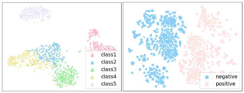
Figure 4: For a 5-way-100-shot task, we visualize the feature descriptors generated by the feature backbone and RankMLP with t-SNE.

Discriminative Ability of Feature Descriptors in RankDNN

We claim that features of the rank-triples formed by the Kronecker are more discriminative and stable than the original deep features. To validate, for a 5-way-100-shot task, we visualize features extracted by the backbone and the second last layer of RankMLP with t-SNE in Fig 4. It can be found that backbone features will result some ambiguity around the classification boundaries. However, the features generated by RankMLP have a stronger discriminative ability in distinguishing positive and negative ranked samples.

Table 5: Ablation study on miniImageNet and CUB using two baselines and under the 5-way-1-shot setting.

Model	miniImageNet	CUB
IE (Rizve et al. 2021)	67.15	80.92
After PCA	65.32	80.11
Feature Differentiation	60.57$\downarrow$	77.33$\downarrow$
Triple Concat	20	20
Pairwise Concat	42.50$\downarrow$	44.65$\downarrow$
Hadamard	65.00$\downarrow$	81.64$\uparrow$
Kronecker	68.72$\uparrow$	82.93$\uparrow$
Polynomial	21.00$\downarrow$	22.00$\downarrow$
S2M2 (Mangla et al. 2020)	64.50	80.68
After PCA	65.32	80.11
Kronecker+RankSVM	60.1$\downarrow$	78.24$\downarrow$
Feature Differentiation	61.24$\downarrow$	77.83$\downarrow$
Hadamard	64.22	79.93$\uparrow$
Kronecker	66.67$\uparrow$	81.78$\uparrow$
The Combined Product	66.88$\uparrow$	81.50$\uparrow$

Ablation Study

Dimension Reduction Module. In Table 5, the 5-way-1-shot/5-way-5-shot classification results of baselines and baselines after the dimension reduction module are obtained from cosine classifiers and linear regression classifiers respectively. It indicates that PCA method will slightly decrease the performance of baselines. Meanwhile, RankDNN can improve the classification accuracies efficiently.

Choices in RankMLP. As in Table 5,first, we verify the effectiveness of RankMLP by replacing RankMLP with RankSVM (Joachims 2002) on S2M2, and the performance on miniImageNet and CUB drops by $4.49\%$ and $2.44\%$ respectively. Second, we explore different triplet encoding schemes by replacing the vector-Kronecker product with feature disparity (Eq. 10), feature concatenation of triplets, feature disparity of pairwise concatenation, Hadamard product (Eq. 11), and the combination of Kronecker and Hadamard products (Eq. 12). We can see that the Kronecker product has the best generalization performance and is applicable to all backbones and datasets. The feature disparity scheme does not well preserve the original feature and sign information and therefore performs poorly. Simply concatenating three feature vectors of a triplet will lead to gradient explosion, and the feature disparity of pairwise concatenation works in low efficiency. Polynomial product fails to describe the similarity information within the triplets, resulting in the subsequent network not being able to learn ranking information. Hadamard product is essentially dot product for vectors and has similar performance as the baseline. However, the combination of Kronecker and Hadamard products can surpass Kronecker product alone in some cases.

$$\psi\left(\left\langle x_{q},x_{i},x_{j}\right\rangle;\theta\right)=\left|{f_{q}}-{f_{i}}\right|-\left|{f_{q}}-{f_{j}}\right|.$$ (10)

$$\psi\left(\left\langle x_{q},x_{i},x_{j}\right\rangle;\theta\right)={f_{q}}\odot{f_{i}}-{f_{q}}\odot{f_{j}}.$$ (11)

$$\psi\left(\left\langle x_{q},x_{i},x_{j}\right\rangle;\theta\right)=({f_{q}}\otimes{f_{i}};{f_{q}}\odot{f_{i}})-({f_{q}}\otimes{f_{j}};{f_{q}}\odot{f_{j}}).$$ (12)

Conclusions

In this paper, we have introduced RankDNN, a novel pipeline for few-shot learning. It can convert a multiclass classification task into a binary ranking relation classification problem. Accurate binary ranking relation classification is made possible by an informative encoding scheme of image triplets and later uses the simple fully connected network to predict whether there are in a query-relevant-irrelevant order or not. Experiments demonstrate the proposed method achieves new state-of-the-art performance on four benchmarks. Meanwhile, experimental results for different backbones and cross-domain settings demonstrate RankDNN is data efficient and domain agnostic.

Supplementary Material

Additional Experiments

Applicability

We tested the applicability of our method to a variety of backbone networks, including Conv-4 (Vinyals et al. 2016), Conv-6(Chen et al. 2019b), ResNet-12 (Rizve et al. 2021), ResNet-18 (Ye et al. 2020), and WRN-28 (Mangla et al. 2020). These backbones serve as the feature extractor in our pipeline.

Table 6: 5-way few-shot classification accuracies of RankDNN on miniImageNet using different backbones.

Backbone	miniImagenet		with RankDNN
	1-shot	5-shot	1-shot	5-shot
Conv-4 (Vinyals et al. 2016)	43.56	53.11	54.20+10.64	66.00+12.89
Conv-6 (Chen et al. 2019b)	46.00	61.50	56.16+10.16	66.77+5.27
ResNet-12 (Rizve et al. 2021)	67.28	84.78	68.72+1.44	85.66+0.88
ResNet-18 (Ye et al. 2020)	55.15	66.78	62.52+7.37	77.33+10.55
WRN (Mangla et al. 2020)	64.93	83.18	66.67+1.74	84.79+1.61

As shown in Table 6, in comparison to the bare backbones, our RankDNN brings over 5% accuracy improvement on Conv-4, Conv-6 and ResNet-18 on both 1-shot and 5-shot. Note that the comparison baseline used in conv-4 is MatchingNet (Vinyals et al. 2016), where the performance of RankDNN improves 10.64% on 1-shot and 12.80% on 5-shot, where it can be proved that RankDNN has superior performance compared with the matching methods in MatchingNet. It also brings over 1% improvement on WRN-28 and ResNet-12. RankDNN can improve the performance of various backbones, especially on 1-shot setting. These results demonstrate the strong robustness of RankDNN.

Table 7: Ablations on learnable parameters of RankDNN.

Model	RankMLP Configurations	Parameters(MB)	miniImagenet
			1-shot	5-shot
Baseline IE	–	–	$67.28$	$84.78$
RankDNN-Lite	$(4096,1024,512,256,1)$	$4.50$	$68.15$	$85.01$
RankDNN	$(6400,1024,512,256,1)$	$6.80$	$68.72$	$85.66$
RankDNN-Large1	$(6400,2048,1024,512,1)$	$14.50$	$68.83$	$85.88$
RankDNN-Large2	$(16384,4096,2048,1024,512,1)$	$74.50$	$71.25$	$85.06$
RankDNN-Large3	$(16384,8000,4000,2000,1000,1)$	$173.09$	$72.07$	$85.11$

Ablation Study on Learnable Parameters and Layers of RankDNN

After feature extraction, we downscaled the original features by different PCA to obtain three input dimensions of RankDNN, including $16,384$, $6,400$, and $4,096$. We designed the corresponding MLPs respectively to explore the relationship between the number of parameters and performance in RankDNN.

Table 8: Comparison of the number of model parameters.

Model	Backbone	Total Param	Backbone Param	Head Param	GFlops	miniImagenet
		(MB)	(MB)	(MB)		1-shot	5-shot
RankDNN(ours)	ResNet-12	19.38	12.47	6.87	182.61	68.72	85.66
XtarNet (Yoon et al. 2020)	ResNet-12	19.87	12.47	7.40	175.92	49.71	60.13
MTL (Sun et al. 2019)	ResNet-12	16.67	12.47	4.20	175.92	$61.20$	$71.50$
wDAE (Gidaris and Komodakis 2019)	WRN	47.52	36.51	11.01	1808.08	$62.96$	$78.85$
FEAT (Ye et al. 2020)	ResNet-18	34.8	33.2	1.6	175.92	$66.78$	$82.05$

Table 9: Ablation study on different choices of the layer numbers in RankMLP. Results of 5-way-1-shot classification are reported.

MLPs	Configurations	mini	tiered
Baseline	ResNet-12	67.28	72.21
One-layer	$(6400,1)$	65.97	70.45
Three-layers	$(6400,512,256,1)$	68.44	73.01
Four-layers	$(6400,1024,512,256,1)$	68.72	73.87
Five-layers	$(6400,2048,1024,512,256,1)$	68.78	73.92

As in Table 7, RankDNN with $173.09M$ parameters get the best result $72.07\%$ on 1-shot. It proves that more learnable parameters in RankMLP lead to better 1-shot classification results. But for 5-shot classification tasks, RankDNN-Large1 performs better. Besides, we found that RankDNN with a large number of parameters cannot continue to improve its performance by fine-tuning on 5-shot tasks. It indicates that RankMLP needs a lot of parameters to learn ranking relationships. But too many parameters still lead to over-fitting during meta-test. The RankDNN with $6.8M$ parameters performs well in both 1-shot and 5-shot tasks and does not consume large amounts of memory.

Also, we tested the choices of different layer numbers in RankMLP. As shown in Table 9, RankMLP using only one-layer cannot learn the ranking relationship well, resulting in lower performance than the baseline. The four-layers MLPs achieve better performances than their three-layers counterparts, especially on tieredImageNet. Compared with the four-layers, the five-layers one has no significant improvement but the number of parameters will be increased by about $6M$ parameters, so the four-layer RankDNN is chosen in the paper.

Ablation Study on Different Testing Methods

During the meta test, we did not fine-tune RankDNN on the 5-way 1-shot setting. However, due to the unique triplets construction, we can construct positive and negative samples of $2,000$ respectively for fine-tuning RankDNN online on the 5-way 5-shot setting. Therefore, we compared the results before and after fine-tuning, as in Table  10. Experiments show that without finetuning, results of RankDNN are even lower than its baseline and after fine-tuning, RankDNN can improve about $2\%$ on 5-way 5-shot on miniImageNet, which demonstrates the validity of the ranking triplets constructed from the Kronecker product and the rapid learning capability of RankDNN. Meanwhile, in order to reduce the test time of ranking voting on K-shot tasks, we average the support features from the same class to one for ranking. And the experiments show that the averaging operation not only reduces the testing time by $>1$s but also improves the performance of RankDNN.

Table 10: Ablation study on different testing methods of 5-shot task on miniImageNet.

Method	Fine-tune	Average	Test time(s)	miniImageNet
Baseline	$\times$	$\times$	0.065	84.78
RankDNN	$\times$	$\times$	1.52	83.20
RankDNN	✓	$\times$	7.58	85.42
RankDNN	$\times$	✓	0.41	83.87
RankDNN	✓	✓	6.46	85.66

Comparison of Learnable Parameters, FLOPs and Accuracies

RankDNN contains a feature backbone and a classification head that increasing 6.87M parameters compared to the feature extraction methods. According to Table 8, compared with other state-of-the-art post-processing methods ,the increased number of parameters and GFlops of RankDNN are in a reasonable range, but the performance of RankDNN is more outstanding.

Table 11: Performance comparison in the cross-domain setting: miniImageNet$\rightarrow$CUB.

Model	miniImageNet $\rightarrow$ CUB
	1-shot	5-shot
SimpleShot ${}_{\;\rm{\,PMLR20}}$	$48.56_{\pm 1.90}$	$65.63_{\pm 1.00}$
GNN+FT${}_{\;\rm{\,ICLR20}}$	$47.47_{\pm 0.90}$	$66.98_{\pm 0.60}$
Afrasiyabi ${}_{\;\rm{\,ECCV20}}$	$46.85_{\pm 0.38}$	$70.37_{\pm 0.35}$
MeTAL${}_{\;\rm{\,ICCV20}}$	–	$70.22_{\pm 0.33}$
FRN${}_{\;\rm{\,CVPR20}}$	$53.39_{\pm 0.47}$	$75.16_{\pm 0.33}$
IE${}_{\;\rm{\,CVPR21}}$	$53.56_{\pm 0.78}$	$75.67_{\pm 0.86}$
RankDNN(ours)	${\bf 60.64_{\pm 0.22}}$	${\bf 85.92_{\pm 0.24}}$

Cross-Domain Few-Shot Classification

We conducted experiments in the cross-domain challenge and compared them with some recent works (Wang et al. 2019b; Chauhan, Nathani, and Kaul 2020) et al, where the model is trained on the miniImageNet and evaluated on the CUB. In this setting, as shown in Table.11, RankDNN improves 7.08$\%$ on 1-shot classification tasks and 10.25% on 5-shot classification tasks over the baseline and significantly exceeds the performance of other methods. These results demonstrate ordering relations within triplets are widely present in all categories and RankDNN has superior migratability and domain agnostic.

Table 12: Performance comparison in other cross-domain settings.

Model	CIFAR $\rightarrow$ CUB	CIFAR $\rightarrow$ mini	mini $\rightarrow$ CIFAR
	1-shot/5-shot	1-shot/5-shot	1-shot/5-shot
Baseline IE	$48.91/58.25$	$55.45/70.45$	$63.77/78.63$
RankDNN(ours)	$54.01/65.00$	$55.33/74.29$	$64.44/80.97$

We also give results of the other three settings, including CIFAR$\rightarrow$ CUB, CIFAR$\rightarrow$ miniImageNet and miniImagenet $\rightarrow$ CIFAR. Compared with the baseline in Table.12, most of the results are improved,especially on the 5-shot setting. This is because in a 5-way 5-shot meta test, RankDNN can adapt the ranking relationships of new categories through fast iterations with a lot of rank samples constructed online. These results demonstrate that RankDNN can learn a unified relevance ranking classifier across different domains and have fast online learning capability for new classes.

Supplementary References

The references not cited in Table 1, 2 and 3 in the main paper are as follows: FRN (Wertheimer, Tang, and Hariharan 2021), DMF (Xu et al. 2021), IEPT (Zhang et al. 2020b), DMN4 (Liu et al. 2022), HGNN (Yu et al. 2022), APP2S (Ma et al. 2022), UNICORN (Ye and Chao 2021), TAS (Le et al. 2021), $\bigtriangleup-$encode (Schwartz et al. 2018), SS (Su, Maji, and Hariharan 2020), Hyperbolic (Khrulkov et al. 2020), PSST (Chen et al. 2021b), CCG+HAN (Gao et al. 2021), PAL (Ma et al. 2021), TPMN (Wu et al. 2021), LH (Jian and Torresani 2022).

References

- Afrasiyabi, Lalonde, and Gagne (2021) Afrasiyabi, A.; Lalonde, J.-F.; and Gagne, C. 2021. Mixture-Based Feature Space Learning for Few-Shot Image Classification. In Proceedings of the IEEE/CVF International Conference on Computer Vision, 9041–9051.
- Arpit et al. (2017) Arpit, D.; Jastrzkbski, S.; Ballas, N.; Krueger, D.; Bengio, E.; Kanwal, M. S.; Maharaj, T.; Fischer, A.; Courville, A.; Bengio, Y.; et al. 2017. A closer look at memorization in deep networks. In International Conference on Machine Learning, 233–242. PMLR.
- Azevedo et al. (2020) Azevedo, A.; Bentes, C.; Castro, M. C.; and Tadonki, C. 2020. Performance Analysis and Optimization of the Vector-Kronecker Product Multiplication. In 2020 IEEE 32nd International Symposium on Computer Architecture and High Performance Computing (SBAC-PAD), 265–272. IEEE.
- Bertinetto et al. (2018) Bertinetto, L.; Henriques, J. F.; Torr, P. H.; and Vedaldi, A. 2018. Meta-learning with differentiable closed-form solvers. arXiv preprint arXiv:1805.08136.
- Briakou and Carpuat (2020) Briakou, E.; and Carpuat, M. 2020. Detecting Fine-Grained Cross-Lingual Semantic Divergences without Supervision by Learning to Rank. arXiv preprint arXiv:2010.03662.
- Broxson (2006) Broxson, B. J. 2006. The kronecker product.
- Burges et al. (2005) Burges, C.; Shaked, T.; Renshaw, E.; Lazier, A.; Deeds, M.; Hamilton, N.; and Hullender, G. 2005. Learning to rank using gradient descent. In Proceedings of the 22nd international conference on Machine learning, 89–96.
- Cakir et al. (2019) Cakir, F.; He, K.; Xia, X.; Kulis, B.; and Sclaroff, S. 2019. Deep metric learning to rank. In Proceedings of the IEEE/CVF Conference on Computer Vision and Pattern Recognition, 1861–1870.
- Chauhan, Nathani, and Kaul (2020) Chauhan, J.; Nathani, D.; and Kaul, M. 2020. Few-shot learning on graphs via super-classes based on graph spectral measures. arXiv preprint arXiv:2002.12815.
- Chen et al. (2019a) Chen, W.-Y.; Liu, Y.-C.; Kira, Z.; Wang, Y.-C.; and Huang, J.-B. 2019a. A Closer Look at Few-shot Classification. In International Conference on Learning Representations.
- Chen et al. (2019b) Chen, W.-Y.; Liu, Y.-C.; Kira, Z.; Wang, Y.-C. F.; and Huang, J.-B. 2019b. A closer look at few-shot classification. arXiv preprint arXiv:1904.04232.
- Chen et al. (2021a) Chen, Y.; Liu, Z.; Xu, H.; Darrell, T.; and Wang, X. 2021a. Meta-Baseline: Exploring Simple Meta-Learning for Few-Shot Learning. In Proceedings of the IEEE/CVF International Conference on Computer Vision, 9062–9071.
- Chen et al. (2021b) Chen, Z.; Ge, J.; Zhan, H.; Huang, S.; and Wang, D. 2021b. Pareto Self-Supervised Training for Few-Shot Learning. In Proceedings of the IEEE/CVF Conference on Computer Vision and Pattern Recognition, 13663–13672.
- De Launey and Seberry (1994) De Launey, W.; and Seberry, J. 1994. The strong Kronecker product. Journal of Combinatorial Theory, Series A, 66(2): 192–213.
- Finn, Abbeel, and Levine (2017) Finn, C.; Abbeel, P.; and Levine, S. 2017. Model-agnostic meta-learning for fast adaptation of deep networks. In International Conference on Machine Learning, 1126–1135. PMLR.
- Gao et al. (2021) Gao, Z.; Wu, Y.; Jia, Y.; and Harandi, M. 2021. Curvature Generation in Curved Spaces for Few-Shot Learning. In Proceedings of the IEEE/CVF International Conference on Computer Vision, 8691–8700.
- Ge (2018) Ge, W. 2018. Deep metric learning with hierarchical triplet loss. In Proceedings of the European Conference on Computer Vision (ECCV), 269–285.
- Gidaris and Komodakis (2018) Gidaris, S.; and Komodakis, N. 2018. Dynamic few-shot visual learning without forgetting. In Proceedings of the IEEE Conference on Computer Vision and Pattern Recognition, 4367–4375.
- Gidaris and Komodakis (2019) Gidaris, S.; and Komodakis, N. 2019. Generating classification weights with gnn denoising autoencoders for few-shot learning. In Proceedings of the IEEE/CVF conference on computer vision and pattern recognition, 21–30.
- He et al. (2016) He, K.; Zhang, X.; Ren, S.; and Sun, J. 2016. Deep residual learning for image recognition. In Proceedings of the IEEE conference on computer vision and pattern recognition, 770–778.
- Hong et al. (2021) Hong, J.; Fang, P.; Li, W.; Zhang, T.; Simon, C.; Harandi, M.; and Petersson, L. 2021. Reinforced attention for few-shot learning and beyond. In Proceedings of the IEEE/CVF Conference on Computer Vision and Pattern Recognition, 913–923.
- Jamal and Qi (2019) Jamal, M. A.; and Qi, G.-J. 2019. Task Agnostic Meta-Learning for Few-Shot Learning. In Proceedings of the IEEE Conference on Computer Vision and Pattern Recognition, 11719–11727.
- Jian and Torresani (2022) Jian, Y.; and Torresani, L. 2022. Label hallucination for few-shot classification. In Proceedings of the AAAI Conference on Artificial Intelligence, volume 36, 7005–7014.
- Joachims (2002) Joachims, T. 2002. Optimizing search engines using clickthrough data. In Proceedings of the eighth ACM SIGKDD international conference on Knowledge discovery and data mining, 133–142.
- Kang et al. (2021) Kang, D.; Kwon, H.; Min, J.; and Cho, M. 2021. Relational Embedding for Few-Shot Classification. In Proceedings of the IEEE/CVF International Conference on Computer Vision, 8822–8833.
- Khrulkov et al. (2020) Khrulkov, V.; Mirvakhabova, L.; Ustinova, E.; Oseledets, I.; and Lempitsky, V. 2020. Hyperbolic image embeddings. In Proceedings of the IEEE/CVF Conference on Computer Vision and Pattern Recognition, 6418–6428.
- Kim et al. (2019) Kim, J.; Kim, T.; Kim, S.; and Yoo, C. D. 2019. Edge-Labeling Graph Neural Network for Few-shot Learning. In Proceedings of the IEEE Conference on Computer Vision and Pattern Recognition, 11–20.
- Krizhevsky, Hinton et al. (2009) Krizhevsky, A.; Hinton, G.; et al. 2009. Learning multiple layers of features from tiny images.
- Langville and Stewart (2004) Langville, A. N.; and Stewart, W. J. 2004. The Kronecker product and stochastic automata networks. Journal of computational and applied mathematics, 167(2): 429–447.
- Le et al. (2021) Le, C. P.; Dong, J.; Soltani, M.; and Tarokh, V. 2021. Task Affinity with Maximum Bipartite Matching in Few-Shot Learning. arXiv preprint arXiv:2110.02399.
- Levi et al. (2021) Levi, E.; Xiao, T.; Wang, X.; and Darrell, T. 2021. Rethinking Preventing Class-Collapsing in Metric Learning With Margin-Based Losses. In Proceedings of the IEEE/CVF International Conference on Computer Vision, 10316–10325.
- Li, Wu, and Burges (2007) Li, P.; Wu, Q.; and Burges, C. 2007. Mcrank: Learning to rank using multiple classification and gradient boosting. Advances in neural information processing systems, 20: 897–904.
- Liu et al. (2021) Liu, C.; Yu, H.; Li, B.; Shen, Z.; Gao, Z.; Ren, P.; Xie, X.; Cui, L.; and Miao, C. 2021. Noise-resistant Deep Metric Learning with Ranking-based Instance Selection. In Proceedings of the IEEE/CVF Conference on Computer Vision and Pattern Recognition, 6811–6820.
- Liu, Schiele, and Sun (2020) Liu, Y.; Schiele, B.; and Sun, Q. 2020. An ensemble of epoch-wise empirical bayes for few-shot learning. In European Conference on Computer Vision, 404–421. Springer.
- Liu et al. (2022) Liu, Y.; Zheng, T.; Song, J.; Cai, D.; and He, X. 2022. Dmn4: Few-shot learning via discriminative mutual nearest neighbor neural network. In Proceedings of the AAAI Conference on Artificial Intelligence, volume 36, 1828–1836.
- Lu et al. (2020) Lu, J.; Gong, P.; Ye, J.; and Zhang, C. 2020. Learning from Very Few Samples: A Survey. arXiv preprint arXiv:2009.02653.
- Ma et al. (2021) Ma, J.; Xie, H.; Han, G.; Chang, S.-F.; Galstyan, A.; and Abd-Almageed, W. 2021. Partner-Assisted Learning for Few-Shot Image Classification. In Proceedings of the IEEE/CVF International Conference on Computer Vision, 10573–10582.
- Ma et al. (2022) Ma, R.; Fang, P.; Drummond, T.; and Harandi, M. 2022. Adaptive poincaré point to set distance for few-shot classification. In Proceedings of the AAAI Conference on Artificial Intelligence, volume 36, 1926–1934.
- Mamut and Vumar (2008) Mamut, A.; and Vumar, E. 2008. Vertex vulnerability parameters of Kronecker products of complete graphs. Information Processing Letters, 106(6): 258–262.
- Mangla et al. (2020) Mangla, P.; Kumari, N.; Sinha, A.; Singh, M.; Krishnamurthy, B.; and Balasubramanian, V. N. 2020. Charting the right manifold: Manifold mixup for few-shot learning. In Proceedings of the IEEE/CVF Winter Conference on Applications of Computer Vision, 2218–2227.
- Masuda (2003) Masuda, K. 2003. A ranking model of proximal and structural text retrieval based on region algebra. In The Companion Volume to the Proceedings of 41st Annual Meeting of the Association for Computational Linguistics, 50–57.
- Palangi et al. (2016) Palangi, H.; Deng, L.; Shen, Y.; Gao, J.; He, X.; Chen, J.; Song, X.; and Ward, R. 2016. Deep sentence embedding using long short-term memory networks: Analysis and application to information retrieval. IEEE/ACM Transactions on Audio, Speech, and Language Processing, 24(4): 694–707.
- Pang et al. (2017) Pang, L.; Lan, Y.; Guo, J.; Xu, J.; Xu, J.; and Cheng, X. 2017. Deeprank: A new deep architecture for relevance ranking in information retrieval. In Proceedings of the 2017 ACM on Conference on Information and Knowledge Management, 257–266.
- Prosser et al. (2010) Prosser, B. J.; Zheng, W.-S.; Gong, S.; Xiang, T.; Mary, Q.; et al. 2010. Person re-identification by support vector ranking. In BMVC, volume 2, 6. Citeseer.
- Qiao et al. (2018) Qiao, S.; Liu, C.; Shen, W.; and Yuille, A. L. 2018. Few-shot image recognition by predicting parameters from activations. In Proceedings of the IEEE Conference on Computer Vision and Pattern Recognition, 7229–7238.
- Rizve et al. (2021) Rizve, M. N.; Khan, S.; Khan, F. S.; and Shah, M. 2021. Exploring Complementary Strengths of Invariant and Equivariant Representations for Few-Shot Learning. In Proceedings of the IEEE/CVF Conference on Computer Vision and Pattern Recognition, 10836–10846.
- Russakovsky et al. (2015) Russakovsky, O.; Deng, J.; Su, H.; Krause, J.; Satheesh, S.; Ma, S.; Huang, Z.; Karpathy, A.; Khosla, A.; Bernstein, M.; et al. 2015. Imagenet large scale visual recognition challenge. International journal of computer vision, 115(3): 211–252.
- Schwartz et al. (2018) Schwartz, E.; Karlinsky, L.; Shtok, J.; Harary, S.; Marder, M.; Kumar, A.; Feris, R.; Giryes, R.; and Bronstein, A. 2018. Delta-encoder: an effective sample synthesis method for few-shot object recognition. In Advances in Neural Information Processing Systems, 2845–2855.
- Shashua, Levin et al. (2003) Shashua, A.; Levin, A.; et al. 2003. Ranking with large margin principle: Two approaches. Advances in neural information processing systems, 961–968.
- Snell, Swersky, and Zemel (2017) Snell, J.; Swersky, K.; and Zemel, R. 2017. Prototypical networks for few-shot learning. In Advances in Neural Information Processing Systems, 4077–4087.
- Su, Maji, and Hariharan (2020) Su, J.-C.; Maji, S.; and Hariharan, B. 2020. When does self-supervision improve few-shot learning? In European conference on computer vision, 645–666. Springer.
- Sun et al. (2019) Sun, Q.; Liu, Y.; Chua, T.-S.; and Schiele, B. 2019. Meta-transfer learning for few-shot learning. In Proceedings of the IEEE/CVF Conference on Computer Vision and Pattern Recognition, 403–412.
- Sung et al. (2018) Sung, F.; Yang, Y.; Zhang, L.; Xiang, T.; Torr, P. H.; and Hospedales, T. M. 2018. Learning to compare: Relation network for few-shot learning. In Proceedings of the IEEE conference on computer vision and pattern recognition, 1199–1208.
- Tang et al. (2021) Tang, S.; Chen, D.; Bai, L.; Liu, K.; Ge, Y.; and Ouyang, W. 2021. Mutual CRF-GNN for Few-Shot Learning. In Proceedings of the IEEE/CVF Conference on Computer Vision and Pattern Recognition, 2329–2339.
- Tian et al. (2020) Tian, Y.; Wang, Y.; Krishnan, D.; Tenenbaum, J. B.; and Isola, P. 2020. Rethinking few-shot image classification: a good embedding is all you need? In Computer Vision–ECCV 2020: 16th European Conference, Glasgow, UK, August 23–28, 2020, Proceedings, Part XIV 16, 266–282. Springer.
- Vinyals et al. (2016) Vinyals, O.; Blundell, C.; Lillicrap, T.; Wierstra, D.; et al. 2016. Matching networks for one shot learning. Advances in neural information processing systems, 29: 3630–3638.
- Wah et al. (2011) Wah, C.; Branson, S.; Welinder, P.; Perona, P.; and Belongie, S. 2011. The caltech-ucsd birds-200-2011 dataset.
- Wang et al. (2019a) Wang, X.; Hua, Y.; Kodirov, E.; Hu, G.; Garnier, R.; and Robertson, N. M. 2019a. Ranked list loss for deep metric learning. In Proceedings of the IEEE/CVF Conference on Computer Vision and Pattern Recognition, 5207–5216.
- Wang et al. (2020) Wang, X.; Zhang, H.; Huang, W.; and Scott, M. R. 2020. Cross-batch memory for embedding learning. In Proceedings of the IEEE/CVF Conference on Computer Vision and Pattern Recognition, 6388–6397.
- Wang et al. (2019b) Wang, Y.; Chao, W.-L.; Weinberger, K. Q.; and van der Maaten, L. 2019b. Simpleshot: Revisiting nearest-neighbor classification for few-shot learning. arXiv preprint arXiv:1911.04623.
- Weichsel (1962) Weichsel, P. M. 1962. The Kronecker product of graphs. Proceedings of the American mathematical society, 13(1): 47–52.
- Wertheimer, Tang, and Hariharan (2021) Wertheimer, D.; Tang, L.; and Hariharan, B. 2021. Few-Shot Classification With Feature Map Reconstruction Networks. In Proceedings of the IEEE/CVF Conference on Computer Vision and Pattern Recognition, 8012–8021.
- Wu et al. (2021) Wu, J.; Zhang, T.; Zhang, Y.; and Wu, F. 2021. Task-Aware Part Mining Network for Few-Shot Learning. In Proceedings of the IEEE/CVF International Conference on Computer Vision, 8433–8442.
- Xu et al. (2021) Xu, C.; Fu, Y.; Liu, C.; Wang, C.; Li, J.; Huang, F.; Zhang, L.; and Xue, X. 2021. Learning Dynamic Alignment via Meta-filter for Few-shot Learning. In Proceedings of the IEEE/CVF Conference on Computer Vision and Pattern Recognition, 5182–5191.
- Yang et al. (2004) Yang, J.; Zhang, D.; Frangi, A. F.; and Yang, J.-y. 2004. Two-dimensional PCA: a new approach to appearance-based face representation and recognition. IEEE transactions on pattern analysis and machine intelligence, 26(1): 131–137.
- Yang, Liu, and Xu (2021) Yang, S.; Liu, L.; and Xu, M. 2021. Free lunch for few-shot learning: Distribution calibration. arXiv preprint arXiv:2101.06395.
- Ye and Chao (2021) Ye, H.-J.; and Chao, W.-L. 2021. How to train your MAML to excel in few-shot classification. arXiv preprint arXiv:2106.16245.
- Ye et al. (2020) Ye, H.-J.; Hu, H.; Zhan, D.-C.; and Sha, F. 2020. Few-shot learning via embedding adaptation with set-to-set functions. In Proceedings of the IEEE/CVF Conference on Computer Vision and Pattern Recognition, 8808–8817.
- Yoon et al. (2020) Yoon, S. W.; Kim, D.-Y.; Seo, J.; and Moon, J. 2020. Xtarnet: Learning to extract task-adaptive representation for incremental few-shot learning. In International Conference on Machine Learning, 10852–10860. PMLR.
- Yu et al. (2022) Yu, T.; He, S.; Song, Y.-Z.; and Xiang, T. 2022. Hybrid Graph Neural Networks for Few-Shot Learning. In Proceedings of the AAAI Conference on Artificial Intelligence, volume 36, 3179–3187.
- Zagoruyko and Komodakis (2016) Zagoruyko, S.; and Komodakis, N. 2016. Wide residual networks. arXiv preprint arXiv:1605.07146.
- Zhang et al. (2021) Zhang, C.; Bengio, S.; Hardt, M.; Recht, B.; and Vinyals, O. 2021. Understanding deep learning (still) requires rethinking generalization. Communications of the ACM, 64(3): 107–115.
- Zhang et al. (2020a) Zhang, C.; Cai, Y.; Lin, G.; and Shen, C. 2020a. DeepEMD: Few-Shot Image Classification With Differentiable Earth Mover’s Distance and Structured Classifiers. In Proceedings of the IEEE/CVF conference on computer vision and pattern recognition, 12203–12213.
- Zhang and van Genabith (2020) Zhang, J.; and van Genabith, J. 2020. Translation Quality Estimation by Jointly Learning to Score and Rank. In Proceedings of the 2020 Conference on Empirical Methods in Natural Language Processing (EMNLP), 2592–2598.
- Zhang et al. (2020b) Zhang, M.; Zhang, J.; Lu, Z.; Xiang, T.; Ding, M.; and Huang, S. 2020b. IEPT: Instance-level and episode-level pretext tasks for few-shot learning. In International Conference on Learning Representations.