Fermionic CFTs at large charge and large N

1 Introduction

The large-charge expansion ([1], see [2] for a review) has been very successfully applied to the critical O(2N) vector model and other bosonic models as a way of making strongly coupled cft analytically accessible. Working in a sector of large charge allows writing an eft (eft) as an expansion in the large charge and computing the cft data [3, 4, 5, 6, 7, 8, 9, 10, 11, 12, 13, 14, 15, 16, 17, 18].

In these models, the ground state at large charge spontaneously breaks the global symmetry, giving rise to a condensate and Goldstone bosons in terms of which the eft is expressed. In the O(2N) model in $D=3$, the operator dimension of the lowest operator of charge $Q$ has the form [1, 9]

$$\Delta(Q)=c_{3/2}Q^{3/2}+c_{1/2}Q^{1/2}-0.0937+\order{Q^{-1/2}},$$ (1.1)

where the first two terms are due to the large-charge ground state, while the $Q^{0}$ contribution stems from the Casimir energy of the conformal Goldstone. While the Wilsonian coefficients $c_{i}$ are not accessible within the eft, working in a limit of large $N$ and large charge allows their computation [19]. The massless spectrum over the superfluid ground state consists of a conformal Goldstone and $N-1$ Goldstone bosons with quadratic dispersion relation:

$$\omega_{\text{conf}} =\frac{1}{\sqrt{2}}p+\dots, \omega_{\text{non-rel}} =\frac{p^{2}}{2\mu}+\dots,$$ (1.2)

each paired with a massive mode with mass of order $\mu\sim\sqrt{Q}$.

While the bulk of the large-charge literature is concerned with bosonic systems, few forays have been made into the world of fermions [20, 14, 21]. In [14] it was found that the superfluid paradigm does not apply to the free fermion case, where sectors of fixed charge are described by Fermi surfaces.

In this article, we want to further close this gap in knowledge and systematically study a number of models with four-fermion interactions in three dimensions, such as the gn (gn) model, the chiral gn model or njl (njl) model, and its $SU(2)\times SU(2)$ generalization. Similarly to [19], we work also here in the limit of large number of fermion flavors, $N\to\infty$, in order to have a controlled setting.

We find that two types of qualitative behaviors are possible. In the gn model there is no ssb (ssb) in sectors of large baryon number, the large-N physics is the one of an approximate Fermi surface in the strict infinite-N limit. We have not yet determined whether the Fermi surface persists once subleading large-N corrections are included. The four-fermi interactions of the njl models instead allow for ssb to occur in specific sectors with large “chiral" charge. In this case, the usual mechanism is at play, and we can verify the expectations from the large-charge eft.

We want to stress that the lack of ssb in the gn model at large charge at leading order in $N$ can be explained in principle in two different ways:

• the four-Fermi interaction is repulsive in every channel and the large-$N$ ground state is a Fermi surface. This would be the first non-free example of this behavior at large charge.;

• the four-Fermi interaction has an attractive channel, runs logarithmically to strong coupling, has a bcs (bcs) condensate and a gap in the fermion sector of order $\exp(-1/g_{\text{eff}})$, where $g_{\text{eff}}$ is the effective coupling at the cutoff. Since $g_{\text{eff}}$ should be of order $1/N$, this means the condensate and the gap would be exponentially small and invisible to all orders in large-$N$ perturbation theory.

Regardless of the presence of ssb, finite-density ground states for critical theories on the cylinder compute the scaling dimension of certain cft primary operators. This fact is a consequence of the state-operator correspondence: a primary $\mathcal{O}_{Q}$ with $U(1)$-charge $Q$ and scaling dimension $\Delta(Q)$ corresponds to a state $|\mathcal{O}_{Q}\rangle$ on a cylinder of radius $r_{0}$ with total charge $Q$ and energy:

$$E(Q)=\Delta(Q)/r_{0}.$$ (1.3)

In particular, if $\mathcal{O}_{Q}$ is the lightest primary of charge $Q$, its corresponding state is known to minimize the combination $\braket{\mathcal{O}_{Q}}{\hat{H}_{\text{cyl}}-\mu\hat{Q}}{\mathcal{O}_{Q}}$ where $\hat{H}_{\text{cyl}}$ is the cft cylinder Hamiltonian and $\hat{Q}$ is the charge operator. A convenient way of selecting such a state is to consider the thermal cft on $S^{1}_{\beta}\times S^{2}$ and study the zero-temperature limit of its grand-canonical partition function,

$$Z(\beta,\mu)=\Tr\left[e^{-\beta(\hat{H}_{\text{cyl}}-\mu\hat{Q})}\right]\xrightarrow[]{\beta\rightarrow\infty}\braket{\mathcal{O}_{Q}}{\mathcal{O}_{Q}}e^{-\beta(E(Q)-\mu Q)}.$$ (1.4)

In the models investigated in the present work, the partition function $Z(\beta,\mu)$ has a path-integral representation which can be computed exactly order-by-order in the large-$N$ limit. In general, it will take the form

$$Z(\beta,\mu)\xrightarrow[N\rightarrow\infty]{\beta\rightarrow\infty}e^{-\beta\Omega(\mu)},$$ (1.5)

where $\Omega$ is the thermodynamic potential. Comparing with Eq. (1.4), we can compute the charge and energy of the state $\ket{\mathcal{O}_{Q}}$ as follows:

$${Q} =-\frac{\partial{\Omega}}{\partial\mu}, {E}(Q) =\left.{\Omega}(\mu)+\mu{Q}\right|_{\mu=\mu({Q})}.$$ (1.6)

When we perform computations on $S^{1}_{\beta}\times T^{2}$ we will use the same symbols to indicate energy and charge density, and normalize by the volume $V$ of the torus. In what follows we will not distinguish between a torus of large volume and flat space.

In the fermion models analysed in this paper, we employ the usual large-N technology and perform a Hubbard–Stratonovich transformation, introducing a complex scalar collective dof (dof) $\Phi$, reducing 4-fermion terms to Yukawa–type interactions. If $\Phi$ is kept non-dynamical, the conformal phase is found in the uv (uv) and is only treatable in the context of the large-$N$ expansion. If $\Phi$ is made dynamical, we obtain the $D=3$ uv completion of these models, and the same conformal phase arises in the ir (ir). Independently on the realization chosen, the large-charge primary $\mathcal{O}_{Q}$ is part of this cft spectrum.

In the njl model, at leading order in $N$, we find the scaling dimension of the operator $\mathcal{O}_{Q}$ to be

$$\frac{\Delta_{SF}(Q)}{2N}=\frac{2}{3}\pqty*{\frac{Q}{2N\kappa_{0}}}^{3/2}+\frac{1}{6}\pqty*{\frac{Q}{2N\kappa_{0}}}^{1/2}-0.0937+\frac{11-6\kappa_{0}^{2}}{720\kappa_{0}^{2}}\pqty*{\frac{Q}{2N\kappa_{0}}}^{-1/2}+\dots$$ (1.7)

in the regime $Q/N\gg 1$, where $\kappa_{0}$ is a constant defined by $\kappa_{0}\tanh\kappa_{0}=1$. This matches the result of the eft superfluid description, as it was the case for the scalar $O(2N)$ model [19] but with different Wilsonian coefficients. While we haven’t computed the full scaling dimension $\Delta(Q)$ to subleading order in $1/N$, we have verified that the corresponding ground state has the expected conformal Goldstone boson excitation. This guarantees that $\Delta(Q)$ will have the universal $Q^{0}$ contribution stemming from its Casimir energy. In large-$N$, we also have access to the opposite regime $Q/N\ll 1$, where one finds

$$\frac{\Delta(Q)}{2N}=\frac{1}{2}\left(\frac{Q}{2N}\right)+\frac{2}{\pi^{2}}\left(\frac{Q}{2N}\right)^{2}+\dots\,,$$ (1.8)

which matches the standard perturbative result for the $Q$-th power of a scalar operator of charge two and dimension one. We find equivalent results for large-charge sectors of the $SU(2)\times SU(2)$ generalization of the njl model.

Both the gn and njl models are expected to have interacting fixed points in any dimension $2<D<4$. Although we will not address the $\epsilon$ expansion in the present work or the behavior of the models in any dimension other than $D=3$, many details of the Lagrangians of these theories can be understood by dimensionally reducing the gn and njl Lagrangians from $D=4$. This being the case, we will often write details of the Lagrangian and discuss the symmetry groups in quasi-four-dimensional language, using the notation $\Gamma_{5}$ for the four-dimensional chirality matrix and $C_{4}$ for the four-dimensional charge-conjugation matrix. We also refer to chiral and axial symmetries, even though these dimensionally reduce to ordinary global symmetries in $D=3$. This language is intended to make it simpler to discuss the corresponding computation in $D=4-\epsilon$, which we hope to address in future work. The use of four-dimensional language in the present paper should be understood in this context, and our conventions are summarised in Appendix A.

In all fermionic models supporting a superfluid ground state at large charge, there is a way to understand the appearance of the condensate in intuitive physical terms. For example, in the njl model one can perform a pg (pg) transformation [29, 30],

$$\Psi\mapsto\frac{1}{2}\left[(1-\Gamma_{5})\Psi-(1+\Gamma_{5})C_{4}\bar{\Psi}^{T}\right], \bar{\Psi}\mapsto\frac{1}{2}\left[\bar{\Psi}(1+\Gamma_{5})-\Psi^{T}C_{4}(1-\Gamma_{5})\right],$$ (1.9)

to a model with a Cooper-type interaction [31, 32]. All computations can be repeated in the Cooper model leading to the same results. The advantage of this model is that the nature of the condensate becomes obvious even in large-$N$: it is a condensate of Cooper pairs, describing a superconductor. The attractive interaction gives rise to a Cooper instability, and we effectively have again a system of condensing bosons at large charge, explaining the similarity of our results to those of the $O(2N)$ scalar model.

The plan of this article is as follows. In Section 2, we introduce all the fermionic models we want to study here. In Section 3, we work in flat space, which is enough to establish the presence or absence of a condensate at large charge in the various models. In Section 4, we compute the spectrum of fluctuations by studying the one-loop propagator of the scalar fields. We discuss the expected eft spectrum and match the results to known Goldstone bosons counting rules. In Section 5, we give the conformal dimensions of the lowest operator of charge Q for the various models, both in the limit of large and small Q. We end with conclusions and an outlook in Section 6. Appendix A contains our conventions and notation for gamma matrices and Dirac spinors (Appendix A.1), the reducible representation we are using for 3$D$ fermions (Appendix A.3) and spinors on $S^{1}_{\beta}\times S^{2}$ (Appendix A.2). In Appendix B, we discuss the Pauli–Gürsey transformation. In Appendix C, we collect some Matsubara sums and loop integrals and compute the one-loop propagator for the njl model.

2 The Models

We focus on fermionic models in three-dimensional Euclidean space which admit a second-order critical phase and are computable in the large-$N$ limit, since we want to take advantage of the controlled setting the large-N limit provides. We focus on a few explicit examples with small symmetry groups .

Our models are all obtained by deforming the free fermion cft by a four-fermion interaction with (irrelevant) coupling $g$. If we assume this model to have a fundamental uv scale $\Lambda$ (given by some fundamental lattice discretization) then at zero temperature and zero density the irrelevant coupling has a critical value $g_{c}^{-1}\sim\Lambda$ where we find a scale-invariant theory separating two phases in which some symmetries are spontaneously broken. Our goal is to study such a critical limit at finite charge density. If we wish to take a formal continuum limit $\Lambda\rightarrow\infty$ for this type of models, we run into the issue that these models are not renormalizable, as the coupling $g$ is irrelevant. It is known, however, that they are renormalizable in the $1/N$ expansion [33]: the corresponding rg (rg) flow joins the free fermion cft in the ir to the conformal phase at $g_{c}$ in the uv. There is evidence that these conformal phases survive in the finite-$N$ regime, but a proper rg treatment requires some type of uv completion. These completions are typically found by introducing extra scalar degrees of freedom interacting with fermionic matter via a Yukawa coupling [34]. The advantage is that Yukawa couplings are relevant in $D<4$, so these models are uv free and strongly interacting in the ir, where one finds the same cft of the four-fermi models. This cft becomes weakly coupled in $D=4-\epsilon$, allowing for perturbative computations of its conformal data (see [21] for a computation at large charge in this regime). Working on large-$N$ models it is sufficient to consider the minimal models with only fermion matter, so we will only briefly comment on the uv complete version.

The models we focus on are the gn model and the njl model together with its minimal $SU(2)\times SU(2)$ generalization. Typically, these models are investigated either in $D=4-\epsilon$ and $D=2+\epsilon$ dimensions at fixed values of $N$, or then for $2<D<4$ in the limit of large $N$. Of course there is no natural notion of chirality in three dimensions. The standard approach is to dimensionally reduce the four-dimensional model and keep using four-component fermions. A Dirac fermion in $D=3+1$ can be decomposed into two Majorana fermions, and in $D=3$, a four-component fermion sits in a reducible representation so that, starting from $N$ Dirac fermions in $D=4$, we obtain $4N$ Majorana fermions in $D=3$. However, there exist two inequivalent two-dimensional representations of the Clifford algebra in $D=3$ (which we will indentify as $\pm\gamma_{\mu}$), so there are $2N+1$ possible inequivalent choices for $4N$ Majorana fermions. In practice there are two interesting situations (which, confusingly enough, are both called gn model in the literature [35]): either all the Majorana fermions sit in the same representation and the system has a $O(4N)$ global symmetry, or half of the fermions sit in one representation and the other half in the other, so that the global symmetry is $O(2N)\times O(2N)\times\mathbb{Z}_{2}$. In the former case there cannot be parity invariance (which is present in four dimensions) because all the spinors have the same eigenvalue for the operator $\gamma_{0}\gamma_{1}\gamma_{2}$. For this reason in the following we will make the latter (parity-invariant) choice, since we are interested in the dimensional reduction of the parity-invariant four-dimensional model. Concretely, this means that we will use four-dimensional reducible gamma matrices of the form

$$\Gamma_{\mu}=\sigma_{3}\otimes\gamma_{\mu}=\begin{pmatrix}\gamma_{\mu}&0\\ 0&-\gamma_{\mu}\end{pmatrix}.$$ (2.1)

In this way it is possible to define a $\Gamma_{5}$ matrix and a notion of chirality (which is actually a flavor symmetry) in three dimensions (see Appendix A.3 for details).

It has been shown that results from $4-\epsilon$ and $2+\epsilon$ expansions at fixed $N$ are completely consistent with the $1/N$ expansion for general dimension, which includes $D=3$ [36]. Moreover, the conformal phases found are known (or strongly believed, e.g. from lattice studies [37]) to exist also in three dimensions and finite $N$.

Gross–Neveu model.

The gn model [38] in the four-dimensional reducible representation we employed is described by the Lagrangian

$$L=\sum_{i=1}^{N}\bar{\Psi}_{i}\Gamma^{\mu}\mathop{\mathrm{{}\partial}}\mathopen{}_{\mu}\Psi_{i}-\frac{g}{N}\left(\sum_{i=1}^{N}\bar{\Psi}_{i}\Psi_{i}\right)^{2},$$ (2.2)

which has a $O(2N)\times O(2N)\times\mathbb{Z}_{2}$ symmetry. We will denote its diagonal Abelian subgroup as $U(1)_{B}$:

$$U(1)_{B}:\Psi_{i}\to e^{i\alpha}\Psi_{i}.$$ (2.3)

The standard large-$N$ analysis is carried out by introducing an auxiliary Stratonovich field $\sigma$ which takes the place of the $\bar{\Psi}\Psi$ bilinear. The resulting Lagrangian is

$$L=\sum_{i=1}^{N}\bar{\Psi}_{i}\left(\Gamma^{\mu}\mathop{\mathrm{{}\partial}}\mathopen{}_{\mu}+\sigma\right)\Psi_{i}+\frac{N}{4g}\sigma^{2}.$$ (2.4)

The critical limit of this theory is found by neglecting the $\sigma^{2}$ term, and corresponds to a second-order phase transition separating phases of broken and unbroken $\mathbb{Z}_{2}$ chiral symmetry acting as $\Psi\rightarrow-\Gamma_{5}\Psi$. At finite $N$, the appropriate uv completion is a Gross–Neveu–Yukawa theory obtained by promoting the $\sigma$ field to a dynamical field:

$$L=\sum_{i=1}^{N}\bar{\Psi}_{i}\left(\Gamma^{\mu}\mathop{\mathrm{{}\partial}}\mathopen{}_{\mu}+\sigma\right)\Psi_{i}+\frac{1}{2g_{Y}}\partial_{\mu}\sigma\partial_{\mu}\sigma.$$ (2.5)

In the ir limit, $g_{Y}$ is relevant and grows large, formally reproducing the same critical action as the gn model. The critical point is weakly coupled in the $4-\epsilon$ expansion, allowing a finite-$N$ study of the gn critical phase.

Nambu–Jona–Lasinio–type models.

The njl model is a time-honored model of four-Fermi interactions with continuous chiral symmetry in four dimensions. Its Lagrangian reads

$$L=\sum_{i=1}^{N}\bar{\Psi}_{i}\Gamma^{\mu}\mathop{\mathrm{{}\partial}}\mathopen{}_{\mu}\Psi_{i}-\frac{g}{N}\left[\left(\sum_{i=1}^{N}\bar{\Psi}_{i}\Psi_{i}\right)^{2}-\left(\sum_{i=1}^{N}\bar{\Psi}_{i}\Gamma_{5}\Psi_{i}\right)^{2}\right]$$ (2.6)

The $\bar{\Psi}\Gamma_{5}\Psi$ bilinear is $Sp(2N)$-invariant, thus the total symmetry group is reduced with respect to the gn model (2.2) to $[O(2N)\times O(2N)]\cap Sp(2N)=U(N)$. On top of the $U(1)_{B}$ symmetry there is an extra $U(1)_{A}$ that extends the $\mathbb{Z}_{2}$ of the gn model, and arises when the different quartic interactions are combined exactly as in $\eqref{eq:L-NJL}$:

$$\Psi_{i}\to e^{i\alpha\Gamma_{5}}\Psi_{i}.$$ (2.7)

The critical phase of the njl model separates two phases in which $U(1)_{A}$ is either broken or unbroken. In the former phase, a Goldstone boson arises, differently to what happens in the gn model where the symmetry is discrete.

Already in the original papers [39, 40], the symmetry group was generalized to a $U(1)_{B}\times SU(2)_{L}\times SU(2)_{R}$ symmetry by considering two-flavor fermions $\Psi_{i,f}$, $f=1,2$ with the Lagrangian

$$L=\sum_{i=1}^{N}\sum_{f=1}^{2}\bar{\Psi}_{i,f}\Gamma^{\mu}\mathop{\mathrm{{}\partial}}\mathopen{}_{\mu}\Psi_{i,f}-\frac{g}{N}\left[\left(\sum_{i=1}^{N}\sum_{f=1}^{2}\bar{\Psi}_{i,f}\Psi_{i,f}\right)^{2}-\sum_{a=1}^{3}\left(\sum_{i=1}^{N}\sum_{f=1}^{2}\bar{\Psi}_{i,f}\Gamma_{5}\sigma^{a}_{fg}\Psi_{i,g}\right)^{2}\right],$$ (2.8)

where the $\sigma^{a}$ are Pauli matrices. This model does not have an $U(1)_{A}$ symmetry. The group $SU(2)_{L}\times SU(2)_{R}$ acts on the fermion fields as

$$\Psi_{i,f} \to e^{i\frac{1+\Gamma_{5}}{2}\omega_{a}^{L}\sigma^{a}_{fg}}\Psi_{i,g} \Psi_{i,f} \to e^{i\frac{1-\Gamma_{5}}{2}\omega_{a}^{R}\sigma^{a}_{fg}}\Psi_{i,g}.$$ and (2.9)

This symmetry is present thanks to the pseudo-real character of $SU(2)$, for which there is no totally symmetric symbol $d_{abc}$. In the present work we will focus on the $U(1)_{B}\times U(1)_{A}$ and $U(1)_{B}\times SU(2)_{L}\times SU(2)_{R}$ njl models, referred respectively as $U(1)$-njl and $SU(2)$-njl, and take the large-$N$ limit using the unbroken $SU(N)$ group factor present in both models. At finite $N$, these are tractable in $d=2+\epsilon$ and around $d=4-\epsilon$ via their known uv completions. For the $U(1)$-njl this is

$$L=\bar{\Psi}\left[\Gamma^{\mu}\mathop{\mathrm{{}\partial}}\mathopen{}_{\mu}+\Phi\left(\tfrac{1+\Gamma_{5}}{2}\right)+\Phi^{*}\left(\tfrac{1-\Gamma_{5}}{2}\right)\right]\Psi+\frac{1}{g_{Y}}\mathop{\mathrm{{}\partial}}\mathopen{}_{\mu}\Phi^{*}\mathop{\mathrm{{}\partial}}\mathopen{}_{\mu}\Phi,$$ (2.10)

with the $U(1)_{A}$ chiral symmetry realized as

$$\Psi \to e^{i\alpha\Gamma_{5}}\Psi, \Phi \to e^{-2i\alpha}\Phi.$$ (2.11)

As in the gn model, the ir limit $g_{Y}\rightarrow\infty$ formally produces the critical action used also in large-$N$ analysis. The field $\Phi$ is then identified with the Stratonovich field for the complex bilinear $\bar{\Psi}\Psi+\bar{\Psi}\Gamma_{5}\Psi$.

A similar completion is found for the $SU(2)$-njl model by introducing a set of real fields $\sigma,\pi_{a=1,2,3}$, so that the uv Lagrangian is

$$L=\bar{\Psi}\left[\Gamma^{\mu}\mathop{\mathrm{{}\partial}}\mathopen{}_{\mu}+\sigma+i\pi_{a}\sigma^{a}\Gamma_{5}\right]\Psi+\frac{1}{2g_{Y}}(\mathop{\mathrm{{}\partial}}\mathopen{}_{\mu}\sigma\mathop{\mathrm{{}\partial}}\mathopen{}_{\mu}\sigma+\mathop{\mathrm{{}\partial}}\mathopen{}_{\mu}\pi^{a}\mathop{\mathrm{{}\partial}}\mathopen{}_{\mu}\pi^{a}).$$ (2.12)

In this model, the symmetry $SU(2)_{L}\times SU(2)_{R}$ acts infinitesimally as

$$\delta_{L,R}\Psi =i\left(\frac{1\pm\Gamma_{5}}{2}\right)\omega_{a}\sigma^{a}\Psi, \begin{cases}\delta_{L,R}\sigma=\pm\omega_{a}\pi_{a},\\ \delta_{L,R}\pi_{a}=\mp\omega_{a}\sigma+\epsilon_{abc}\pi_{b}\omega_{c}.\end{cases}$$ (2.13)

Equivalently, in terms of the field $\Phi=\sigma+\pi_{a}\sigma^{a}$, we have the following finite transformations

$$\begin{cases}\Psi\to e^{i\frac{1+\Gamma_{5}}{2}\omega_{a}\sigma^{a}}\Psi,\\ \Phi\to\Phi e^{-i\omega_{a}\sigma^{a}},\end{cases} \begin{cases}\Psi\to e^{i\frac{1-\Gamma_{5}}{2}\omega^{\prime}_{a}\sigma^{a}}\Psi,\\ \Phi\to e^{i\omega^{\prime}_{a}\sigma^{a}}\Phi.\end{cases}$$ (2.14)

This model was originally discussed by Nambu and Jona–Lasinio and is also known as the isonjl model.

Cooper model.

Both the gn-type and njl-type models exhibit a fermion-antifermion interaction. Often, especially in the context of condensed matter physics, one wants to consider a difermion interaction in order to study superconductivity (arising via Cooper pairing). Large-$N$ Fermionic models intended for the description of superconductivity at finite $U(1)_{B}$-charge density generally include an interaction term of the form

$$(4f)_{Cp}=\frac{g}{N}\bar{\Psi}C\bar{\Psi}^{T}\,\Psi^{T}C\Psi,$$ (2.15)

in addition to gn-type or njl-type interactions [41, 32]. In particular, we are interested in the model with just the Cooper pair interaction term,

$$L=\bar{\Psi}\Gamma^{\mu}\mathop{\mathrm{{}\partial}}\mathopen{}_{\mu}\Psi+\frac{g}{N}\bar{\Psi}C_{4}\bar{\Psi}^{T}\,\Psi^{T}C_{4}\Psi.$$ (2.16)

In our notation, we have $C_{4}=\Gamma_{2}$, see also Appendix A.3. At criticality — differently to what happens in gn model — this model exhibits a non-trivial solution to the gap equation at zero temperature and finite $U(1)_{B}$-chemical potential giving rise to a superconducting phase.
It turns out that this model is dual to the njl model in the sense of [32]. This can be seen by applying the Pauli–Gürsey transformation [29, 30, 31],

$$\Psi\mapsto\frac{1}{2}\left[(1-\Gamma_{5})\Psi-(1+\Gamma_{5})C_{4}\bar{\Psi}^{T}\right], \bar{\Psi}\mapsto\frac{1}{2}\left[\bar{\Psi}(1+\Gamma_{5})-\Psi^{T}C_{4}(1-\Gamma_{5})\right].$$ (2.17)

For a more detailed discussion of this transformation we refer to Appendix B. A few remarks are in order here:

• Both the Cooper model and the njl model have a $U(1)_{A}\times U(1)_{B}$ symmetry. Under a pg transformation the $U(1)_{B}$-chemical potential in the Cooper model is mapped into the $U(1)_{A}$-chemical potential of the njl model and vice versa. This means that any result obtained in the njl model at finite $U(1)_{A}$ chemical potential will also apply to the Cooper model at finite $U(1)_{B}$ chemical potential.

• It is possible to compute relevant quantities at the critical point of both the Cooper model and the njl model, which should agree up to a pg transformation. We have explicitly checked this matching for the leading-$N$ ground state energy at finite $U(1)_{B}$-chemical potential in the Cooper model and $U(1)_{A}$-chemical potential of the njl model.

• The pg transformation corresponds to a linear involution at the level of the path-integral. Therefore, it only affects the path integral measure up to a trivial rescaling.

3 Symmetry breaking at large $N$

Whether or not the large-charge approach leads to simplifications depends crucially on the appearance of a condensate in the large-charge sector. We therefore first discuss symmetry breaking in the various models we consider.

3.1 Gross–Neveu model

As a warm-up we consider the gn model with $2N$ three-dimensional Dirac fermions at finite temperature and finite $U(1)_{B}$-chemical potential $\mu$. Using the reducible representation given in Appendix A.3 and introducing the auxiliary field $\sigma$ for the $\bar{\Psi}\Psi$ bilinear, its action reads

$$S=\int_{S^{1}_{\beta}\times\mathbb{R}^{2}}\left[\bar{\Psi}(\Gamma^{\mu}\partial_{\mu}-\mu\Gamma_{3}+\sigma)\Psi+\frac{N}{4g}\sigma^{2}\right].$$ (3.1)

The model is equipped with a cutoff scale $\Lambda$. For generic values of the parameters $(g,\beta,\mu)$ the $\sigma$ field can acquire a vev (vev), spontaneously breaking the discrete parity symmetry $\Psi\rightarrow-\Gamma_{5}\Psi$. Under generic assumptions, the $\sigma$-vev configuration can be taken to be homogeneous $\langle\sigma\rangle=\sigma_{0}$. The large-$N$ effective action for $\sigma$ can be obtained expanding around this saddle as $\sigma=\sigma_{0}+\hat{\sigma}/\sqrt{N}$:

$$S_{\text{eff}}=N\left\{\beta V\frac{\sigma_{0}^{2}}{4g}-\Tr\log\big{(}D^{(\mu)}\big{)}^{-1}\right\}+\frac{1}{2}\left[\Tr(D^{(\mu)}\hat{\sigma}D^{(\mu)}\hat{\sigma})+\frac{1}{4g}\int_{S^{1}_{\beta}\times\mathbb{R}^{2}}\hat{\sigma}^{2}\right]+\mathcal{O}(N^{-1}),$$ (3.2)

where we introduced the fermionic propagator at finite chemical potential

$$D^{(\mu)}(X,Y)=\braket{X}{(\Gamma^{\mu}\partial_{\mu}-\mu\Gamma_{3}+\sigma_{0})^{-1}}{Y}.$$ (3.3)

Leading-order action and gap equation

The value of the condensate $\sigma_{0}$ is found by minimizing the zero-order action. Using the momentum-space representation of the propagator and the fermionic Matsubara summation in Appendix C one finds the expression for the grand potential

$$\frac{\Omega}{N}\coloneqq\frac{\sigma_{0}^{2}}{4g}-2\int^{\Lambda}\frac{\dd^{2}p}{(2\pi)^{2}}\left\{\omega_{p}+\frac{1}{\beta}\log\left(1+e^{-\beta(\omega_{p}+\mu)}\right)+(\mu\leftrightarrow-\mu)\right\},$$ (3.4)

where we introduced $\omega_{p}^{2}=p^{2}+\sigma_{0}^{2}$. For consistency we need to assume $\sigma_{0},\mu\ll\Lambda$. We can then introduce the critical coupling $g_{c}^{-1}=\Lambda/\pi$ so that when $\sigma_{0}\neq 0$ the gap equation reads

$$0=\left(\frac{1}{g}-\frac{1}{g_{c}}\right)-\frac{1}{\pi}\left(\sigma_{0}-\frac{1}{\beta}\log(1+e^{\beta(\sigma_{0}+\mu)})-\frac{1}{\beta}\log(1+e^{\beta(\sigma_{0}-\mu)})\right).$$ (3.5)

Its solution $\sigma_{0}$ is obtained in closed form as

$$e^{\beta\sigma_{0}}=\frac{1}{2}\left\{e^{\beta\pi\left(\frac{1}{g_{c}}-\frac{1}{g}\right)}-2\cosh\beta\mu+\sqrt{\left(e^{\beta\pi\left(\frac{1}{g_{c}}-\frac{1}{g}\right)}-2\cosh\beta\mu\right)^{2}-4}\right\}.$$ (3.6)

At zero chemical potential, $\mu=0$, there is a non-trivial solution in the zero-temperature limit $\beta\rightarrow\infty$ only for $g>g_{c}$. It reads

$$\eval*{\sigma_{0}}_{\mu,\beta^{-1}=0}=\pi\left(\frac{1}{g_{c}}-\frac{1}{g}\right).$$ (3.7)

This is the known second-order quantum phase transition of the large-$N$ gn model at $g=g_{c}$, separating the parity-broken and the parity-unbroken phase. Outside criticality $g>g_{c}$, this solution survives at zero temperature and finite chemical potential as long as $\mu<\mu_{c}=\sigma_{0}\big{|}_{\mu,\beta^{-1}=0}$ and for $\mu>\mu_{c}$ parity is restored. At the quantum critical point $g=g_{c}$ there is no non-vanishing solution for any $\mu$. As we will discuss in Section 5, this is consistent with the fact that in the cft the chemical potential is sourcing a parity-even primary operator.

The zero-temperature ground state in the critical limit is then a filled Fermi sphere of massless fermions $\sigma_{0}=0$. The leading-order action $S^{(0)}$ gives its grand potential

$$\frac{\Omega}{N}=-2\int_{\mu<|p|<\Lambda}\frac{\dd^{2}p}{(2\pi)^{2}}\omega_{p}-2\mu\int_{|p|<\mu}\frac{\dd^{2}p}{(2\pi)^{2}}=-\frac{\Lambda^{3}}{3\pi}-\frac{\mu^{3}}{6\pi}.$$ (3.8)

The $U(1)_{B}$-charge and (renormalized) energy density of this Fermi-sphere ground state are computed using Eq. (1.6) and read

$$\frac{Q}{N} =\frac{\mu^{2}}{2\pi}, \frac{E}{N} =\frac{1}{3\pi}\pqty*{2\pi\frac{Q}{N}}^{3/2}.$$ (3.9)

This expression is computing the leading order in the large-$Q$ expansion for the scaling dimension $\Delta_{FS}$ of the Fermi sphere operator [14], which is the lightest primary of charge $Q$. In fact, there is no difference with the free fermion cft result at this order.

We would like to stress that it is not clear at this point what is the implication of the absence of ssb at leading order in the large-$N$ limit. Interactions between fermions are suppressed by the coupling $g_{\text{eff}}=\order{1/N}$ going to zero at large $N$, so at infinite $N$ the ground state is described by an exactly free Fermi surface. At finite $N$, interaction corrections to the free-fermi operator dimensions can in principle be studied in the framework of the Fermi surface eft [42], with the corrections organized in a $1/Q$ expansion corresponding to the low-energy expansion in powers of $1/\mu^{2}R^{2}$, in addition to their large-$N$ suppression.

One logical possibility is that the physics remais the one of a weakly-interacting Fermi surface at the lowest energies. However, this is not the only possibility, since the Fermi surface at finite N is never exactly free, and unlike the case of the superfluid efts studied in [1, 43], interactions in the Fermi surface are not automatically suppressed at low energies. As it is well-known, the effect of the four-Fermi interaction on the excitations above the Fermi surface runs logarithmically [42], running to strong coupling as $g_{\text{eff}}\propto\log(\mu/E_{\text{IR}})$ if there is any attractive four-fermi channel. This suggests that at an infrared scale of $R^{-1}=E_{\text{IR}}\sim\exp(-(\text{constant})/g_{\text{UV}})\mu=\exp(-(\text{constant})\times N)\mu$, the Fermi surface may always develop a condensate of Cooper pairs, leading to a gap in the fermion sector of order $E_{\text{gap}}\sim\exp(-(\text{ constant})\times N)\sqrt{Q}/R$. This scenario would be somewhat generic, and would predict the low-lying large-charge operator dimensions to be described by a purely bosonic superfluid eft, but only for ultra-large values of the charge exponentially large in $Q$ so that the enhancement of the gap by $\sqrt{Q}$ could overcome the exponential suppression in $N$.

As we have not done an analysis of the four-fermi interaction about the Fermi surface ground state, we do not know which of these two possibilities is realized; we leave that as a question to be answered in the future.

3.2 Nambu–Jona–Lasinio model

Next, we consider the $U(1)_{A}\times U(1)_{B}$ njl model at finite $U(1)_{A}$-chemical potential. Introducing the appropriate Stratonovich field $\Phi$, the action reads

$$S=\int_{S^{1}_{\beta}\times\mathbb{R}^{2}}\left[\bar{\Psi}\left(\Gamma^{\mu}\partial_{\mu}-\mu\Gamma_{3}\Gamma_{5}+\Phi P_{+}+\bar{\Phi}P_{-}\right)\Psi+\frac{N}{4g}\abs{\Phi}^{2}\right],$$ (3.10)

where $P_{\pm}=(1\pm\Gamma_{5})/2$ are the chiral projectors. This chemical potential is sourcing a finite charge density for the symmetry

$$\Psi \to e^{i\alpha\Gamma_{5}}\Psi, \Phi \to e^{-2i\alpha}\Phi.$$ (3.11)

The leading-$N$ thermodynamic potential density for constant configurations of the $\Phi$ field is found as

$$\frac{\Omega}{N}=\frac{\abs{\Phi_{0}}^{2}}{4g}-\int^{\Lambda}\frac{\dd^{2}p}{(2\pi)^{2}}\left\{\Omega_{+}+\Omega_{-}+\frac{2}{\beta}\log\left(1+e^{-\beta\Omega_{+}}\right)+\frac{2}{\beta}\log\left(1+e^{-\beta\Omega_{-}}\right)\right\},$$ (3.12)

where we introduced the one-particle on-shell energies

$$\Omega_{\pm}^{2}\coloneqq\abs{\Phi_{0}}^{2}+(\abs{p}\pm\mu)^{2}.$$ (3.13)

The novelty with respect to the gn model discussed above is that no Fermi sphere can arise if $\Phi_{0}\neq 0$, since $\Omega_{\pm}\geq 0$. If this is the case, we can neglect the thermal logarithm terms in the zero-temperature limit, and obtain

$$\lim_{\beta\rightarrow\infty}\frac{\Omega}{N}=\frac{\abs{\Phi_{0}}^{2}}{4g}-\int^{\Lambda}\frac{\dd^{2}p}{(2\pi)^{2}}\bqty*{\sqrt{(\abs{p}+\mu)^{2}+\abs{\Phi_{0}}^{2}}+\sqrt{(\abs{p}-\mu)^{2}+\abs{\Phi_{0}}^{2}}}.$$ (3.14)

Introducing the critical coupling $g_{c}^{-1}=\Lambda/\pi$, the gap equation for the $\Phi$ field at zero temperature reads

$$0=\frac{\mathop{\mathrm{{}\partial}}\mathopen{}^{2}\Omega}{\mathop{\mathrm{{}\partial}}\mathopen{}\abs{\Phi_{0}}^{2}}=\frac{1}{2}\left(\frac{1}{g}-\frac{1}{g_{c}}\right)+\frac{1}{2\pi^{2}}\left[\sqrt{\abs{\Phi_{0}}^{2}+\mu^{2}}-\mu\arctanh*(\frac{\mu}{\sqrt{\abs{\Phi_{0}}^{2}+\mu^{2}}})\right].$$ (3.15)

Since this equation depends only on $\abs{\Phi_{0}}$, we can look for a real and positive vev $\braket{\Phi}=\Phi_{0}>0$. In the critical limit $g=g_{c}$ there is always a non-trivial solution to the gap equation at finite chemical potential, which reads

$$\Phi_{0}=\mu\sqrt{\kappa_{0}^{2}-1},$$ (3.16)

where $\kappa_{0}$ is the solution to the equation $\kappa_{0}\tanh\kappa_{0}=1$, and numerically, $\Phi_{0}/\mu=0.6627\dots$.

This solution implies that the finite-$\mu$ ground state spontaneously breaks the $U(1)_{A}$ symmetry by giving a vev to the auxiliary field $\Phi$, which then plays the role of the order parameter. Symmetry restoration only occurs at $\mu=0$, as conformal symmetry prohibits the existence of a new scale separating the broken and unbroken phase. This situation becomes more explicit if one computes the renormalized potential $\Omega$ for general constant configurations of $\Phi$. Since the divergent part of $\Omega$ is $\mu$-independent, we can compute its minimal subtraction

$$\frac{\Omega(\mu)}{N}-\frac{\Omega(0)}{N} =-\int\frac{\dd^{2}p}{(2\pi)^{2}}\left[\Omega_{+}+\Omega_{-}-2\sqrt{p^{2}+\abs{\Phi}^{2}}\right]$$ (3.17)

$$=-\frac{1}{6\pi}\left[3\abs{\Phi}^{2}\mu\arctanh*(\tfrac{\mu}{\sqrt{\abs{\Phi}^{2}+\mu^{2}}})+(\mu^{2}-2\abs{\Phi}^{2})\sqrt{\abs{\Phi}^{2}+\mu^{2}}+2\abs{\Phi}^{3}\right],$$

and add again its renormalized value $\Omega$. This is precisely the same integral that we had solved in the computation for the gn model and reads

$$\Omega(0)=\frac{N\abs{\Phi}^{3}}{3\pi}.$$ (3.18)

Finally the renormalized potential reads

$$\frac{\Omega}{N}=-\frac{1}{6\pi}\left[3\abs{\Phi}^{2}\mu\arctanh*(\tfrac{\mu}{\sqrt{\abs{\Phi}^{2}+\mu^{2}}})+(\mu^{2}-2\abs{\Phi}^{2})\sqrt{\abs{\Phi}^{2}+\mu^{2}}\right].$$ (3.19)

This potential is $U(1)_{A}$-invariant as expected, but has a $S^{1}$-worth of vacua at $\abs{\Phi}=\mu\sqrt{\kappa_{0}^{2}-1}$. In Figure 1 we plot it for $\mathop{Im}\Phi=0$ for different values of the chemical potential.

Figure 1: Leading-order in $N$ thermodynamic potential for the NJL model as function of $\Phi$ for different values of $\mu$. For $\mu>0$ the minima at $\Phi\neq 0$ signal spontaneous symmetry breaking.

The ground state we obtain for this model corresponds to a superfluid with $U(1)_{A}$-charge and energy density, respectively

$$\frac{Q}{N} =\frac{\kappa_{0}^{3}\mu^{2}}{2\pi}, \frac{E}{N} =\frac{1}{3\pi\kappa_{0}^{3/2}}\pqty*{2\pi\frac{Q}{N}}^{3/2}.$$ (3.20)

As we will discuss in section 5, this ground state energy is computing the leading order in the large-charge expansion for the scaling dimension $\Delta_{SF}$ of the operator $\mathcal{O}_{SF}$ corresponding to a superfluid ground state. No Fermi sphere arises in this sector and all the charge is contained in the superfluid.

One might wonder whether a superfluid ground state is found also at finite $U(1)_{B}$-charge. In that case, instead of the eigenvalues given in Eq. (3.13) one obtains

$$\Omega_{\pm}=\sqrt{p^{2}+\abs{\Phi_{0}}^{2}}\pm\mu.$$ (3.21)

These are the same eigenvalues appearing in the gn model, so we can conclude that in this sector no superfluid arises, but instead one has a Fermi sphere with charge and energy density as in Eq. (3.9).

3.3 $SU(2)_{L}\times SU(2)_{R}$ Nambu-Jona-Lasinio model

Finally, we consider the $SU(2)_{L}\times SU(2)_{R}$ njl model. In this case we have multiple choices for charge densities to source. Let us first consider the model at finite chemical potential for the $\sigma^{3}$ and $\Gamma_{5}\sigma^{3}$ generators. The critical action reads

$$S=\int_{S^{1}_{\beta}\times\mathbb{R}^{2}}\left[\bar{\Psi}\left(\Gamma^{\mu}\partial_{\mu}+\sigma+i\pi_{a}\sigma^{a}\Gamma_{5}-\left\{\begin{aligned} &\mu_{V}\Gamma_{3}\sigma^{3}\\ &\mu_{A}\Gamma_{3}\Gamma_{5}\sigma^{3}\end{aligned}\right\}\right)\Psi\right].$$ (3.22)

In this case, the thermodynamic potential is found to be

$$\frac{\Omega^{V,A}}{N}=-2\int^{\Lambda}\frac{\dd^{2}p}{(2\pi)^{2}}\left\{\Omega_{+}^{V,A}+\Omega_{-}^{V,A}+\frac{2}{\beta}\log\left(1+e^{-\beta\Omega_{+}^{V,A}}\right)+\frac{2}{\beta}\log\left(1+e^{-\beta\Omega_{+}^{V,A}}\right)\right\},$$ (3.23)

where we introduced the one-particle on-shell energies

$$\Omega^{V}_{\pm} =\sqrt{|\Phi_{2}|^{2}+\left(\sqrt{(|p|+|\Phi_{1}|}\pm\mu_{V}\right)^{2}}, \Omega^{A}_{\pm} =\sqrt{|\Phi_{1}|^{2}+\left(\sqrt{(|p|+|\Phi_{2}|}\pm\mu_{A}\right)^{2}},$$ (3.24)

with $|\Phi_{1}|^{2}=\sigma^{2}+\pi_{3}^{2},\,|\Phi_{2}|^{2}=\pi_{1}^{2}+\pi_{2}^{2}$. In both cases, there is no solution for the zero-temperature gap equation in which both field combinations $\Phi_{1},\Phi_{2}$ acquire a vev. When $\mu_{V}$ is turned on, one finds the solution $|\Phi_{1,0}|=0,\,|\Phi_{2,0}|=\mu_{V,A}\sqrt{\kappa_{0}^{2}-1}$, where $\kappa_{0}$ is the same transcendental number found in the $U(1)$-njl model (3.16). The same holds when $\mu_{A}$ is turned on, exchanging the vev for $\Phi_{1},\Phi_{2}$.

Since in both cases $\Omega_{\pm}^{V,A}\geq 0$ for any value of $|p|$ and $\mu_{V,A}$, no Fermi sphere arises in the zero-temperature limit, and we find the same superfluid regime of the $U(1)_{B}\times U(1)_{A}$ njl model (3.16). The only difference is an overall factor of 2 in the thermodynamic potential and ground state energy.

We have also computed the ground states for finite left / right chemical potentials $\mu_{L,R}$, which respectively source the charge densities $\bar{\Psi}(1\pm\Gamma_{5})\Gamma_{3}\sigma^{3}\Psi$. We find that the ground state is a filled Fermi sphere in both cases, just like in the gn model and no ssb arises.

4 Spectrum of fluctuations

After having identified the large-charge ground state in the last section, we now study the spectrum of fluctuations over it, still working in flat space. In the cases with symmetry breaking, we expect, based on the superfluid eft for the O(N) model at large charge the appearance of a conformal Goldstone with a dispersion relation $\omega=p/\sqrt{2}+\dots$ paired with a massive mode of order $\mu$ in all cases [1]. On the other hand, in the gn model, the ground state is a filled Fermi sphere and since no Goldstone bosons arise, the eft predictions do not apply.

4.1 GN model

The fluctuations around the Fermi sphere ground state can be both fermionic or bosonic. The fermionic fluctuations are of the particle-hole type, as it also happens in the free fermion critical theory. Bosonic fluctuations are instead due to the composite field $\sigma$. To understand their effect on the ground state, we need to compute the effective propagator of the $\sigma$ field in the unbroken phase $\sigma_{0}=0$ at criticality. This can be read off the nlo effective action $S^{(2)}_{\text{eff}}$ in Eq. (3.2). It is convenient to compute this action in momentum space, where

$$\Tr(D^{(\mu)}\sigma D^{(\mu)}\sigma) =-\operatorname*{\mathchoice{\ooalign{$\displaystyle\sum$\cr$\displaystyle\int$\cr}}{\ooalign{\raisebox{0.14pt}{\scalebox{0.7}{$\textstyle\sum$}}\cr$\textstyle\int$\cr}}{\ooalign{\raisebox{0.2pt}{\scalebox{0.6}{$\scriptstyle\sum$}}\cr$\scriptstyle\int$\cr}}{\ooalign{\raisebox{0.2pt}{\scalebox{0.6}{$\scriptstyle\sum$}}\cr$\scriptstyle\int$\cr}}}\dd^{2}p\,\sigma(-P)\sigma(P)\operatorname*{\mathchoice{\ooalign{$\displaystyle\sum$\cr$\displaystyle\int$\cr}}{\ooalign{\raisebox{0.14pt}{\scalebox{0.7}{$\textstyle\sum$}}\cr$\textstyle\int$\cr}}{\ooalign{\raisebox{0.2pt}{\scalebox{0.6}{$\scriptstyle\sum$}}\cr$\scriptstyle\int$\cr}}{\ooalign{\raisebox{0.2pt}{\scalebox{0.6}{$\scriptstyle\sum$}}\cr$\scriptstyle\int$\cr}}}\frac{\dd^{2}k}{\beta(2\pi)^{2}}\Tr[D^{(\mu)}(K)D^{(-\mu)}(P-K)].$$ (4.17)

In this expression we made use of the property $D^{(\mu)}(X,Y)=-D^{(-\mu)}(Y,X)$ and the expression for the momentum-space fermionic propagator at finite density,

$$D^{(\mu)}(P) =\frac{i\Gamma_{\mu}\tilde{P}^{\mu}}{\tilde{P}^{2}}, \tilde{P} =(\omega_{n}-i\mu,\vec{p}).$$ (4.18)

The one-loop integral appearing in Eq. (4.17) can be reduced, after some algebra, as

$$\vbox{\hbox{\includegraphics[scale={1}]{GN_diag}}}\,=2P^{2}I_{2}-4I_{1},$$ (4.19)

where $I_{1},I_{2}$ are two master scalar integrals computed in detail in Appendix C. This result is sufficient to obtain the quadratic fluctuation action $S^{(2)}_{\text{eff}}$ in a mass-independent regularization scheme in which the critical coupling is $g_{c}^{-1}=0$. At zero temperature, one finds

$$S^{(2)}_{\text{eff}}=\frac{1}{2}Tr(\sigma D^{(\mu)}\sigma D^{(\mu)})=\frac{1}{2}\operatorname*{\mathchoice{\ooalign{$\displaystyle\sum$\cr$\displaystyle\int$\cr}}{\ooalign{\raisebox{0.14pt}{\scalebox{0.7}{$\textstyle\sum$}}\cr$\textstyle\int$\cr}}{\ooalign{\raisebox{0.2pt}{\scalebox{0.6}{$\scriptstyle\sum$}}\cr$\scriptstyle\int$\cr}}{\ooalign{\raisebox{0.2pt}{\scalebox{0.6}{$\scriptstyle\sum$}}\cr$\scriptstyle\int$\cr}}}\dd^{2}p\,\sigma(-P)\sigma(P)\left[\frac{\sqrt{P^{2}}}{4}+\frac{\mu}{\pi}\right].$$ (4.20)

The non-local action above does not describe stable bosonic fluctuations on top of the Fermi-sphere ground state. In fact, the momentum-independent part cannot be interpreted as a mass term, but rather as a decay constant of order $\sim\mu$, as it is the case in the unbroken phase of the model discussed in [44].

4.2 NJL model

In the previous section, we have seen that fixing the axial charge in the njl model leads to a vev for the field $\Phi$. From the determinant in Eq. (3.14) we see that all the fermions acquire a mass,

$$m_{F}^{2}=\mu^{2}+\Phi_{0}^{2}=\kappa_{0}^{2}\mu^{2}.$$ (4.21)

This shows that the flavor symmetry remains unbroken, while the $U(1)_{A}$ symmetry is broken.

In the present model, the eft prediction can be verified explicitly by computing the $1/N$ term in the expansion of the functional determinant, which gives the propagator for the fluctuations of the collective field $\hat{\Phi}=\hat{\sigma}+i\hat{\pi}$ over the vacuum $\Phi_{0}$.

To identify the spectrum of fluctuations over the condensate, we compute the inverse propagator of the field $\hat{\Phi}$ with one fermion loop. The Lagrangian around the vacuum $\braket{\Phi}=\Phi_{0}$ is

$$L_{\Phi_{0}}=\bar{\Psi}\Gamma_{\mu}\partial^{\mu}\Psi+\Phi_{0}\bar{\Psi}\Psi-\mu\bar{\Psi}\Gamma_{3}\Gamma_{5}\Psi+\frac{1}{\sqrt{N}}(\hat{\sigma}\bar{\Psi}\Psi+i\hat{\pi}\bar{\Psi}\Gamma_{5}\Psi).$$ (4.22)

The fermion propagator is

$$\begin{split}D^{(\mu,\Phi_{0})}(P)&=(-i\not{P}+\Phi_{0}-\mu\Gamma_{3}\Gamma_{5})^{-1}\\ &=\frac{\left(\omega^{2}+k^{2}+\Phi_{0}^{2}-\mu^{2}+2\mu(i\omega\Gamma_{3}+\Phi_{0})\Gamma_{3}\Gamma_{5}\right)}{\left(\omega^{2}+\Phi_{0}^{2}+(\mu+k)^{2}\right)\left(\omega^{2}+\Phi_{0}^{2}+(\mu-k)^{2}\right)}\left(i\not{P}+\Phi_{0}-\mu\Gamma_{3}\Gamma_{5}\right),\end{split}$$ (4.23)

where ${P}=(\omega,\vec{p})$ and $\not{P}=\Gamma^{\mu}P_{\mu}$. Thanks to the absence of a Fermi sphere ground state, we can work directly in the $\beta\rightarrow\infty$ limit and drop all temperature-dependent contributions. This also amounts to considering Matsubara frequencies as continuous $\omega_{n}\rightarrow\omega$. Note that the propagator is properly antisymmetric $D^{(\mu,\Phi_{0})}(-P)=-D^{(-\mu,-\Phi_{0})}(P)$.

Using this fermionic propagator we can obtain the inverse propagator for the scalar fluctuations in terms of the following momentum space integrals:

$$=D^{-1}_{\sigma\sigma}(P)=-\int\frac{\dd^{3}k}{(2\pi)^{3}}\Tr\left[D^{(\mu,\Phi_{0})}(K)D^{(-\mu,-\Phi_{0})}(P-K)\right],$$ (4.24)

$$=D^{-1}_{\sigma\pi}(P)=-i\int\frac{\dd^{3}k}{(2\pi)^{3}}\Tr\left[D^{(\mu,\Phi_{0})}(K)\Gamma_{5}D^{(-\mu,-\Phi_{0})}(P-K)\right],$$ (4.25)

$$=D^{-1}_{\pi\sigma}(P)=-i\int\frac{\dd^{3}k}{(2\pi)^{3}}\Tr\left[\Gamma_{5}D^{(\mu,\Phi_{0})}(K)D^{(-\mu,-\Phi_{0})}(P-K)\right],$$ (4.26)

$$=D^{-1}_{\pi\pi}(P)=\int\frac{\dd^{3}k}{(2\pi)^{3}}\Tr\left[\Gamma_{5}D^{(\mu,\Phi_{0})}(K)\Gamma_{5}D^{(-\mu,-\Phi_{0})}(P-K)\right].$$ (4.27)

All these integrals can be conveniently expanded in the regime of interest $(P/\mu)\ll 1$. The zeroth order corresponds to the $P=0$ result and needs to be regularized by subtracting the $\mu=0$ result, since the divergence is $\mu$-independent (see Appendix C.2). The result is

$$D^{-1}(P)\Big{|}_{\mathcal{O}(0)}=\begin{pmatrix}D^{-1}_{\sigma\sigma}(0)&D^{-1}_{\sigma\pi}(0)\\ D^{-1}_{\pi\sigma}(0)&D^{-1}_{\pi\pi}(0)\end{pmatrix}=\frac{\kappa_{0}\mu}{\pi}\begin{pmatrix}1&0\\ 0&0\end{pmatrix},$$ (4.28)

where $\kappa_{0}$ again satisfies $\kappa_{0}\tanh\kappa_{0}=1$, with $\Phi_{0}=\mu\sqrt{\kappa_{0}^{2}-1}$. This is consistent with a massive and a massless mode. Beyond the zeroth order no regularization is necessary. To linear order in P we find

$$D^{-1}(P)\Big{|}_{\mathcal{O}(P/\mu)}=\frac{\kappa_{0}\omega}{2\pi}\begin{pmatrix}0&-1\\ 1&0\end{pmatrix}.$$ (4.29)

Finally, the quadratic order is computed to be

$$D^{-1}(P)\Big{|}_{\mathcal{O}(P^{2}/\mu^{2})}=\begin{pmatrix}\frac{(2\kappa_{0}^{2}-1)\omega^{2}}{12\pi\kappa_{0}(\kappa_{0}^{2}-1)\mu}+\frac{(3\kappa_{0}^{6}-2\kappa_{0}^{4}-2\kappa_{0}^{2}+2)p^{2}}{24\pi\kappa_{0}^{3}(\kappa^{2}-1)\mu}&0\\ 0&\frac{\kappa_{0}\omega^{2}}{4\pi(\kappa_{0}^{2}-1)\mu}+\frac{\kappa_{0}^{3}p^{2}}{8\pi(\kappa_{0}^{2}-1)\mu}\end{pmatrix}.$$ (4.30)

The dispersion relations of the two modes come from the zero of the inverse propagator given by the matrix

$$D^{-1}(P)=\begin{pmatrix}\frac{\kappa_{0}\mu}{\pi}+\frac{2\kappa_{0}^{2}\left(2\kappa_{0}^{2}-1\right)\omega^{2}+\left(3\kappa_{0}^{6}-2\kappa_{0}^{4}-2\kappa_{0}^{2}+2\right)p^{2}}{24\pi\kappa_{0}^{3}\left(\kappa_{0}^{2}-1\right)\mu}&-\frac{\kappa_{0}}{2\pi}\omega\\ \frac{\kappa_{0}}{2\pi}\omega&\frac{2\kappa_{0}\omega^{2}+\kappa_{0}^{3}p^{2}}{8\pi(\kappa_{0}^{2}-1)\mu}\end{pmatrix}+\mathcal{O}(P^{3}/\mu^{3}),$$ (4.31)

and read

$$\omega_{1}^{2} =-\frac{1}{2}p^{2}+\dots,$$ (4.32)

$$\omega_{2}^{2} =-12\frac{\left(\kappa_{0}^{2}-1\right)\kappa_{0}^{4}}{\left(2\kappa_{0}^{2}-1\right)}\mu^{2}-\frac{\left(5\kappa_{0}^{6}-5\kappa_{0}^{4}-\kappa_{0}^{2}+2\right)}{2\kappa_{0}^{2}(2\kappa_{0}^{2}-1)}p^{2}+\dots$$ (4.33)

From this result, we recognize the expected conformal Goldstone and a radial-type mode of mass of order $\order{\mu}$. This is one of the main results of the present works, and shows that large-charge superfluid efts can apply to this sector. We have performed the same computation for the $SU(2)$-njl at finite chemical potentials $\mu_{A,V}$ and found the same spectrum of (4.32) with two extra degenerate gapped modes with dispersion relation

$$\omega^{2}=-4\kappa_{0}^{2}\mu^{2}-\frac{\left(\kappa_{0}^{2}-1\right)p^{2}}{\kappa_{0}^{2}}+\dots$$ (4.34)

Based on this result, we expect the conformal Goldstone eft to describe the fluctuations on top of the ssb ground state for both the $U(1)$-njl and the $SU(2)$-njl model.

4.3 Symmetry breaking patterns and Goldstones

The analysis performed in the previous section lead to the conclusion that the usual large-charge eft of superfluid gb describes both the ground states studied in the $U(1)$-njl and in the $SU(2)$-njl models. Thus, the large-charge sectors of these two theories are identical and no gb with quadratic dispersion relation is found. This fact is consistent with the known counting rules for gb. Let us consider the formal limit $R\rightarrow\infty$ of the cylinder so that we can label spacetime generators using a flat space notation. The actions (3.10) and (3.22) at zero chemical potentials and at criticality have total symmetry

$$SO(4,1)_{\text{conf}}\times SU(N)\times U(1)_{B}\times\begin{cases}U(1)_{A}&\text{($U(1)$-\acs{njl})}\\ SU(2)_{L}\times SU(2)_{R}&\text{($SU(2)$-\acs{njl}).}\end{cases}$$ (4.35)

Introducing the respective axial chemical potentials $\mu_{A}$, reduces this symmetry to

$$\mathbb{R}_{\tau}\times SO(3)_{\text{rot}}\times SU(N)\times U(1)_{B}\times\begin{cases}U(1)_{A}&\text{($U(1)$-\acs{njl})}\\ U(1)^{(3)}_{A}\times U(1)^{(3)}_{B}&\text{($SU(2)$-\acs{njl}),}\end{cases}$$ (4.36)

where $\mathbb{R}_{\tau}$ is cylinder-time translation and $SO(3)_{\text{rot}}$ are the isometries of the sphere, and $U(1)_{A,B}^{(3)}$ are the global phase symmetries generated by $\Gamma_{5}\sigma^{3}$ and $\sigma^{3}$ respectively (the Cartans of $SU(2)_{L}\times SU(2)_{R}$). In both cases the ground state arising at large-$N$ breaks spontaneously a linear combination of $\mathbb{R}_{\tau}$ and the $U(1)_{A}$ factor. This is the typical setting in which spontaneous symmetry breaking of a global symmetry group occurs in a non-Lorentz invariant theory . In this setting the counting of gb is non-trivial [45, 46, 47, 48], see also [49] for a recent review. The upshot is that the number of broken generators, $n_{BG}$, is related to the number of gb with linear disperions relation, $n_{A}$, and the number of gb with quadratic disperions relation, $n_{B}$, as follows:

$$n_{A}+2n_{B}=n_{BG}.$$ (4.37)

Since both in the $U(1)$-njl and $SU(2)$-njl models we have $n_{BG}=1$, only one gb with linear dispersion relation can appear: the known conformal superfluid phonon. The only difference between the two models is found in the gapped sector: the ground state fluctuation in the $SU(2)$-njl also contains two degenerate gapped modes combined in a complex scalar charged under the unbroken $U(1)_{B}^{(3)}$.

5 Conformal dimensions and local CFT spectrum

So far we have considered four-fermion critical models in flat space, studying their finite-density properties in a large spatial box of volume $V$ (or analogously, on a torus of volume $V$). When instead the system is put on a cylinder $\mathbb{R}\times S^{2}$, the energy of the finite-density ground state corresponds to the scaling dimension of a specific primary of the cft living at the critical point according to the relation $\Delta=r_{0}E_{\text{g.s}}$, where $r_{0}$ is the sphere radius.

Fermionic models can be mapped on $\mathbb{R}\times S^{2}$ via a Weyl transformation, see Appendix A.2. The upshot is that the finite-density kinetic term for fermions reads

$$S =\int_{\mathbb{R}\times S^{2}}\left[\bar{\Psi}(\not{D}-\mu\Gamma_{\tau}+\sigma)\Psi\right] Q =\int_{S^{2}}\bar{\Psi}\Gamma_{\tau}\Psi,$$ with (5.1)

where $\not{D}$ is the Dirac operator on $\mathbb{R}\times S^{2}$.

5.1 GN model

In the large-$N$ gn model the thermodynamic grand potential density on $S^{1}_{\beta}\times S^{2}$, analogous to the one in flat space in Eq. (3.4), is found to be

$$\frac{\Omega}{N}=\frac{\sigma_{0}^{2}}{4g}-\frac{2}{(4\pi r_{0}^{2})}\sum_{j=\frac{1}{2}}(2j+1)\left\{\sqrt{\omega_{j}^{2}+\sigma_{0}^{2}}+\text{thermal contributions}\right\},$$ (5.2)

where $\omega_{j}=(j+1/2)/r_{0}$ are the eigenvalues of the Dirac operator on $S^{2}$. It is easy to see that the gap equation does not admit a non-trivial solution $\sigma_{0}\neq 0$ at criticality $g=g_{c}$ for any value of $\mu$ at zero temperature, exactly as in flat space. The zero-temperature grand potential then reduces to

$$\frac{\Omega}{N}=-\frac{1}{2\pi r_{0}^{2}}\left\{\sum_{\omega_{j}>\mu}(2j+1)\omega_{j}+\mu\sum_{\omega_{j}<\mu}(2j+1)\right\}$$ (5.3)

and describes a Fermi-sphere ground states for massless fermions. The charge and energy density of the Fermi sphere are readily found using Eq. (1.6):

$$\frac{Q}{N} =\frac{1}{2\pi r_{0}^{2}}\lfloor\mu r_{0}\rfloor(\lfloor\mu r_{0}\rfloor+1), \frac{E}{N} =\frac{1}{6\pi r_{0}^{3}}\lfloor\mu r_{0}\rfloor(\lfloor\mu r_{0}\rfloor+1)(2\lfloor\mu r_{0}\rfloor+1).$$ (5.4)

The floor function implements the fact that on the cylinder energy levels are discretized, and for a filled Fermi sphere a chemical potential value in between two energy levels corresponds to the same filled Fermi sphere. The formal macroscopic limit $r_{0}\rightarrow\infty$ reproduces the flat space results in Section 3.1 and is analogous to the large-chemical-potential limit.

This ground state corresponds to the scalar primary operator $\mathcal{O}_{FS}$ which was constructed explicitly in [14] in the free fermion cft, which is parity-even. This is the lowest primary of charge $Q$ even if the cft is an interacting one, due to the fact that the auxiliary field $\sigma$ does not condense. The same conclusion is reached for the njl model at finite $U(1)_{B}$ chemical potential. The $U(1)_{B}$-charge and scaling dimension of $\mathcal{O}_{FS}$ are found to be, respectively,

$$\frac{Q}{2N} =\lfloor\mu r_{0}\rfloor(\lfloor\mu r_{0}\rfloor+1), \frac{\Delta_{FS}}{2N} =\frac{1}{3}\lfloor\mu r_{0}\rfloor(\lfloor\mu r_{0}\rfloor+1)(2\lfloor\mu r_{0}\rfloor+1)=\frac{Q}{6N}\sqrt{\frac{2Q}{N}+1}.$$ (5.5)

Here we have normalized $Q,\Delta_{F}$ by $2N$, the total number of three-dimensional Dirac fermions. The scaling dimension $\Delta_{FS}$ is shown in Figure 2 as a function of $Q$. The $Q\rightarrow\infty$ asymptotics can be systematically computed, and the first few orders are

$$\frac{\Delta_{FS}}{N} =\frac{2}{3}\pqty*{\frac{Q}{2N}}^{3/2}+\frac{1}{12}\pqty*{\frac{Q}{2N}}^{1/2}-\frac{1}{192}\pqty*{\frac{Q}{2N}}^{-1/2}+\order*{\pqty*{\frac{Q}{2N}}^{-3/2}}, \frac{Q}{2N} \rightarrow\infty.$$ (5.6)

For this large-charge sector, we do not have Goldstone fluctuations describing new primaries with $\sim\mathcal{O}(1)$ gap from the Fermi sphere primary. Instead, we have particle-hole excitations creating new (generally spinful and fermionic) primaries with same charge and gap $\delta\Delta\sim\mathcal{O}(1)$. As discussed at the end of Section 4.1, fluctuations of the $\sigma$ field cannot consistently be used to describe new primaries with $\sim\mathcal{O}(1)$ gap from the Fermi-sphere ground state. As this is a large-$N$ result, it would be interesting to see if this effect persists for finite $N$ by and if there can be a description in terms of a Fermi liquid for the eft.

5.2 NJL model

In the $U(1)_{B}\times U(1)_{A}$ njl model, the ground state at finite $U(1)_{A}$-chemical potential corresponds to a superfluid. When the cft is placed on $S^{1}_{\beta}\times S^{2}$, this will compute the scaling dimension $\Delta_{SF}$ of a corresponding primary $\mathcal{O}_{SF}$. Here we treat explicitly the $U(1)_{B}\times U(1)_{A}$ njl model, keeping in mind that the leading-$N$ result for the $SU(2)_{L}\times SU(2)_{R}$ model in Section 3.3 is obtained by replacing $N$ by $2N$.

At criticality, the zero-temperature thermodynamic potential reads

$$\frac{\Omega}{N} =-\frac{1}{(4\pi r_{0}^{2})}\sum_{j=\frac{1}{2}}^{\infty}(2j+1)\left\{\Omega_{+}+\Omega_{-}\right\}, \Omega_{\pm}^{2} =\abs{\Phi}^{2}+(\omega_{j}\pm\mu)^{2},$$ (5.7)

where $\omega_{j}$ are the Dirac eigenvalues on the sphere. Following the same procedure as before, we determine the charge and scaling dimension of the operator $\mathcal{O}_{SF}$ to be

$$\frac{Q}{2N} =\frac{1}{2}\sum_{j=\frac{1}{2}}^{\infty}(2j+1)\left\{\frac{\omega_{j}+\mu}{\Omega_{+}}-\frac{\omega_{j}-\mu}{\Omega_{-}}\right\},$$ (5.8)

$$\frac{\Delta}{2N} =-\frac{r_{0}}{2}\sum_{j=\frac{1}{2}}^{\infty}(2j+1)\left\{\Omega_{+}+\Omega_{-}\right\}+(\mu r_{0})\frac{Q}{2N}.$$ (5.9)

Moreover, the auxiliary field $\Phi$ needs to be evaluated on the solution $\Phi_{0}$ of the gap equation,

$$G\coloneqq\frac{1}{2r_{0}}\left.\sum_{j=\frac{1}{2}}^{\infty}(2j+1)\left\{\frac{1}{\Omega_{+}}+\frac{1}{\Omega_{-}}\right\}\right|_{\Phi=\Phi_{0}}=0.$$ (5.10)

While the charge is finite, the scaling dimension and the gap equation, on the other hand, need to be regularized. This can be done, for example, by removing the leading divergence in the sums and adding them back in a $\zeta$-function regulated form. This leads to the following regulated expressions:

$$G^{\text{reg}} =\frac{1}{2}\sum_{j=\frac{1}{2}}^{\infty}\left\{(2j+1)\frac{1}{r_{0}}\left[\frac{1}{\Omega_{+}}+\frac{1}{\Omega_{-}}\right]-4\right\}+2\zeta(0),$$ (5.11)

$$\frac{\Delta^{\text{reg}}}{2N} =-\frac{1}{2}\sum_{j=\frac{1}{2}}^{\infty}\left\{(2j+1)r_{0}\left[\Omega_{+}+\Omega_{-}\right]-4r_{0}^{2}\omega_{j}^{2}-2r_{0}^{2}\Phi^{2}\right\}-r_{0}^{2}\Phi^{2}\zeta(0)+(\mu r_{0})\frac{Q}{2N}.$$ (5.12)

These regulated expressions can be computed numerically for different values of the charge $Q$, as the infinite sum now converges. The result is plotted in Figure 2 together with the scaling dimension $\hat{\Delta}_{FS}=\Delta_{FS}/2N$ for the operator $\mathcal{O}_{FS}$ appearing both in the gn and njl model at finite $U(1)_{B}$ chemical potential.

The first few terms in the asymptotic expansion of $\Delta_{SF}$ in the regimes $\frac{Q}{N}\gg 1$ and the $\frac{Q}{N}\ll 1$ can also be computed analytically. This is done in the following sections.

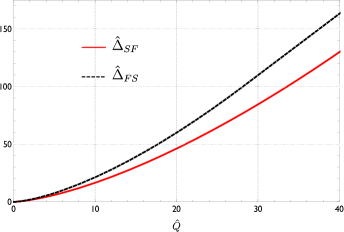
Figure 2: Scaling dimension ${\Delta}_{FS}$ of the Fermi sphere primary $\mathcal{O}_{FS}$ in the GN model and NJL model at finite $U(1)_{B}$-charge density compared with the scaling dimension ${\Delta}_{SF}$ of the superfluid operator $\mathcal{O}_{SF}$ in the NJL model at finite $U(1)_{A}$-charge density.

Large-Q regime

At finite $U(1)_{A}$ charge density, the problem has three dimensionful quantities, $\mu$, $\sigma_{0}$ and $r_{0}$, but in the above equations only the two dimensionless ratios $r_{0}\mu,\,r_{0}\Phi_{0}$ appear. Here, we are interested in the large-charge limit in which $\mu$ is the dominant scale, so that $r_{0}\mu\gg 1$. In this limit, the solution of the gap equation has the expansion

$$\Phi_{0}r_{0}=\sqrt{\kappa_{0}^{2}-1}\left(\mu r_{0}+\frac{\kappa_{1}}{\mu r_{0}}+\frac{\kappa_{2}}{(\mu r_{0})^{3}}+\dots\right).$$ (5.13)

Note that $r_{0}$ enters via the curvature of the sphere which has dimension $[\mathop{Ric}]=2$ and this is why we have an expansion in $r_{0}^{2}$. In order to determine the coefficients $\kappa_{i}$, we need to solve the gap equation:

$$G=G_{r}+G_{d}=0,$$ (5.14)

where we have separated the regular and the divergent parts:

$$G_{r} =\sum_{\ell=1}\ell\left[\frac{1}{\sqrt{(\ell+\mu r_{0})^{2}+(\Phi_{0}r_{0})^{2}}}+\frac{1}{\sqrt{(\ell-\mu r_{0})^{2}+(\Phi_{0}r_{0})^{2}}}-2\frac{1}{\sqrt{\ell^{2}+(\Phi_{0}r_{0})^{2}}}\right],$$ (5.15)

$$G_{d} =2\sum_{\ell=1}\ell\frac{1}{\sqrt{\ell^{2}+(\Phi_{0}r_{0})^{2}}},$$ (5.16)

where we also shifted the summation in Eq. (5.10) as $j=\ell-1/2$. The regular part can be written as an asymptotic expansion in $\mu r_{0}\gg 1$ using the Euler–Maclaurin formula:

$$G_{r}=2\mu r_{0}\left[-\kappa_{0}+\sqrt{\kappa_{0}^{2}-1}+\arccoth(\kappa_{0})\right]+\frac{1}{6\mu r_{0}}\left[-\frac{1}{\kappa_{0}}-12\kappa_{0}\kappa_{1}+\frac{1+12(\kappa_{0}^{2}-1)\kappa_{1}}{\sqrt{\kappa_{0}^{2}-1}}\right]+\dots$$ (5.17)

For the divergent part, we perform $\zeta$-function regularization:

$$G_{d} =2\eval*{\sum_{\ell=1}^{\infty}\ell(\ell^{2}+r_{0}^{2}\Phi_{0}^{2})^{-s}}_{s=1/2}=\eval*{\frac{2}{\Gamma(s)}\int_{0}^{\infty}\frac{\dd{t}}{t}t^{s}\sum_{\ell=1}^{\infty}\ell e^{-(\ell^{2}+r_{0}^{2}\Phi_{0}^{2})t}}_{s=1/2}.$$ (5.18)

In the limit $\mu r_{0}\gg 1$, we also have $\Phi_{0}r_{0}\gg 1$ as is evident from the flat-space result in Eq. (3.16). In the $\zeta$-function regulated expression we can then obtain an expansion for $\Phi_{0}r_{0}\gg 1$ by expanding the integrand around $t=0$, using the standard formula

$$\sum_{\ell=1}^{\infty}\ell e^{-\ell^{2}t}=\frac{e^{-t}}{12}\left(2t+5+\frac{6}{t}+\dots\right),$$ (5.19)

resulting in

$$G_{d}=-2\Phi_{0}r_{0}-\frac{1}{6\Phi_{0}r_{0}}-\frac{1}{120(\Phi_{0}r_{0})^{3}}+\dots.$$ (5.20)

If we now insert the ansatz (5.13) we can solve the equation $G_{d}+G_{r}=0$ order by order in $r_{0}\mu$ and solve for the coefficients $\kappa_{i}$. We then find that the first coefficient, $\kappa_{0}$, satisfies the same irrational equation we had found in Section 3, and appears in all coefficients $\kappa_{i>0}$:

$$\kappa_{0}\tanh\kappa_{0} =1, \kappa_{1} =-\frac{1}{12\kappa_{0}^{2}}, \kappa_{2} =\frac{33-16\kappa_{0}^{2}}{1440\kappa_{0}^{6}}, \dots$$ (5.21)

We apply the same strategy to compute the divergent sum appearing in the scaling dimension (5.9), which coincides with the thermodynamic potential $\Omega/(2N)$: we divide it into the two contributions

$$\Omega_{r} =-2N\sum_{\ell=1}\ell\left[\sqrt{(\ell+\mu r_{0})^{2}+\Phi_{0}^{2}r_{0}^{2}}+\sqrt{(\ell-\mu r_{0})^{2}+\Phi_{0}^{2}r_{0}^{2}}-2\sqrt{\ell^{2}+\Phi_{0}^{2}r_{0}^{2}}\right],$$ (5.22)

$$\Omega_{d} =-4N\sum_{\ell=1}^{\infty}\ell\sqrt{\ell^{2}+\Phi_{0}^{2}r_{0}^{2}}.$$ (5.23)

Using Euler–Maclaurin, the regular part gives, at leading order,

$$\Omega_{r}=-\frac{2N}{3}(r_{0}\mu)^{3}\pqty*{3(\kappa_{0}^{2}-1)\arccoth{\kappa_{0}}+3\kappa_{0}-2\kappa_{0}^{3}+2(\kappa_{0}^{2}-1)^{\frac{3}{2}}}+\dots,$$ (5.24)

while using zeta-function regularization, we find for the divergent part

$$\Omega_{d}=N\pqty*{\frac{4(\Phi_{0}r_{0})^{3}}{3}+\frac{\Phi_{0}r_{0}}{3}-\frac{1}{60\Phi_{0}r_{0}}+\dots}.$$ (5.25)

Finally, we can obtain the relation $\mu=\mu(Q)$ by inverting order-by-order the charge equation in (5.9). As already mentioned, the sum appearing there is convergent, so we can simply apply the Euler–Maclaurin formula. The result of the gap equation (5.13) with the coefficients in (5.21) together with the relation $\mu=\mu(Q)$ lead to the following asymptotic expansion for the scaling dimension $\Delta_{SF}$:

$$\frac{\Delta_{SF}(Q)}{2N}=\frac{2}{3}\pqty*{\frac{Q}{2N\kappa_{0}}}^{3/2}+\frac{1}{6}\pqty*{\frac{Q}{2N\kappa_{0}}}^{1/2}+\frac{11-6\kappa_{0}^{2}}{720\kappa_{0}^{2}}\pqty*{\frac{Q}{2N\kappa_{0}}}^{-1/2}+\dots$$ (5.26)

This is one of the main results of this work. Note that the leading term is consistent with the expression that we had found for the ground state energy in flat space, Eq. (3.20). We can think of the subleading terms in the large-charge expansion as of an expansion in the curvature, so that the leading term just depends on the volume of the manifold, which for the two-sphere is $V=4\pi r_{0}^{2}$.

The conformal Goldstone identified in Sec. 4 is present for any $N$ and gives rise to a universal contribution to the scaling dimension at order $N^{0}$, $Q^{0}$ with the same numerical value as for the $O(N)$ model, see Eq. (1.1). Moreover, its excitations generate the local spectrum on top of the primary $\mathcal{Q}_{Q}$.

Small-Q regime

Next we want to study the limit of $Q/N\ll 1$. At $Q=0$, the free energy has to vanish by conformal invariance as it corresponds to the conformal dimension of the identity operator. In our description in terms of a composite scalar field $\Phi$, we need to take into account its conformal coupling to the curved background. For the three-dimensional cylinder this is the same as a mass term $m=1/(2r_{0})$, which in our description comes from the chemical potential (see [19] for the analogous derivation in the large-N vector model). A direct calculation shows that for $\mu=1/(2r_{0})$ the free energy and the charge both vanish and the gap equation on the sphere is satisfied with a zero, vev $\Phi_{0}=0$. The small-charge expansion has to be done around this point, so it is convenient to write $\mu=1/(2r_{0})+\hat{\mu}$ and expand for small $\hat{\mu}$ all the expressions in Eq. (5.9). At $\hat{\mu}=0$ the symmetry is restored, so $\Phi_{0}$ does not acquire a vev. We can then write an ansatz for $\Phi_{0}$ in the form

$$\hat{\mu}=\mu_{2}\Phi_{0}^{2}r_{0}+\mu_{4}\Phi_{0}^{4}r_{0}^{3}+\dots.$$ (5.27)

The corresponding charge can be computed expanding in $\Phi_{0}r_{0}\ll 1$, and one finds

$$\frac{Q}{2N}= \frac{\pi^{2}}{4}(\Phi_{0}r_{0})^{2}-\frac{\pi^{2}}{16}(\pi^{2}-16\mu_{2})(\Phi_{0}r_{0})^{4}$$

$$+\frac{\pi^{2}}{48}\left(\pi^{4}+12\pi^{2}(\mu_{2}^{2}-2\mu_{2})+48\mu_{4}\right)(\Phi_{0}r_{0})^{6}+\dots,$$ (5.28)

which manifestly vanishes for $\Phi_{0}=0$. The coefficients $\mu_{i}$ appearing in the ansatz (5.27) are determined solving the gap equation (5.10) order by order in small $\hat{\mu}$. Once again, we separate the gap equation into a divergent and a convergent sum as done before, both of them having a well-defined expansion for $\Phi_{0}r_{0}\ll 1$, and this time we subtract the $\hat{\mu}=0$ contribution. The convergent part is

$$G_{r}=\frac{\pi^{2}}{2}\mu_{2}(\Phi_{0}r_{0})^{2}-\frac{\pi^{2}}{4}(\pi^{2}\mu_{2}-4\mu_{2}^{2}-2\mu_{4})(\Phi_{0}r_{0})^{4}+\dots,$$ (5.29)

while the divergent part can be regularized order-by-order using $\zeta$-function regularization as follows:

$$G_{d} =\sum_{\ell=0}^{\infty}(2\ell+1)\frac{1}{\sqrt{(\ell+\tfrac{1}{2})^{2}+(\Phi_{0}r_{0})^{2}}}$$

$$=2\sum_{\ell=0}(\ell+\tfrac{1}{2})\sum_{k=0}\binom{-\nicefrac{{1}}{{2}}}{k}(\Phi_{0}r_{0})^{2k}(\ell+\tfrac{1}{2})^{2(-1/2-k)}$$

$$=2\sum_{k=0}\binom{-\nicefrac{{1}}{{2}}}{k}(\Phi_{0}r_{0})^{2k}\zeta(2k;\tfrac{1}{2})$$

$$=-\frac{\pi^{2}(\Phi_{0}r_{0})^{2}}{2}+\frac{\pi^{4}(\Phi_{0}r_{0})^{4}}{8}+\dots.$$ (5.30)

Solving the gap equation $G_{r}+G_{d}=0$ order by order, we can determine all the coefficients $\mu_{i}$. The first two are given by

$$\mu_{2} =1, \mu_{4} =\frac{\pi^{2}-8}{4}, \dots$$ (5.31)

As done in the previous section, we apply the same procedure to compute the divergent sum appearing in the scaling dimension (5.9), which corresponds to the thermodynamic potential $\Omega/(2N)$. This quantity can be divided in the two contributions

$$\begin{multlined}\Omega_{r}=-2N\sum_{\ell=1}\ell\left[\sqrt{(\ell+\tfrac{1}{2}+\hat{\mu}r_{0})^{2}+(\Phi_{0}r_{0})^{2}}+\sqrt{(\ell-\tfrac{1}{2}-\hat{\mu}r_{0})^{2}+(\Phi_{0}r_{0})^{2}}\right.\\ -\left.\sqrt{(\ell+\tfrac{1}{2})^{2}+(\Phi_{0}r_{0})^{2}}+\sqrt{(\ell-\tfrac{1}{2})^{2}+(\Phi_{0}r_{0})^{2}}\right],\end{multlined}\Omega_{r}=-2N\sum_{\ell=1}\ell\left[\sqrt{(\ell+\tfrac{1}{2}+\hat{\mu}r_{0})^{2}+(\Phi_{0}r_{0})^{2}}+\sqrt{(\ell-\tfrac{1}{2}-\hat{\mu}r_{0})^{2}+(\Phi_{0}r_{0})^{2}}\right.\\ -\left.\sqrt{(\ell+\tfrac{1}{2})^{2}+(\Phi_{0}r_{0})^{2}}+\sqrt{(\ell-\tfrac{1}{2})^{2}+(\Phi_{0}r_{0})^{2}}\right],$$ (5.34)

$$\Omega_{d}=-4N\sum_{\ell=1}^{\infty}(\ell+\tfrac{1}{2})\sqrt{(\ell+\tfrac{1}{2})^{2}+(\Phi_{0}r_{0})^{2}}.$$ (5.35)

The regular part can be expanded for $\Phi_{0}r_{0}\ll 1$ inside the sum, and at leading order one finds

$$\Omega_{r}=N\pqty*{\frac{\pi^{2}}{2}\mu_{2}(\Phi_{0}r_{0})^{4}+\dots}.$$ (5.36)

The divergent part can be regularized using $\zeta$-function regularization:

$$\Omega_{d} =-4N\sum_{\ell=0}^{\infty}(\ell+\tfrac{1}{2})\sum_{k=0}\binom{\nicefrac{{1}}{{2}}}{k}(\Phi_{0}r_{0})^{2k}(\ell+\tfrac{1}{2})^{2(1/2-k)}$$ (5.37)

$$=-4N\sum_{k=0}\binom{\nicefrac{{1}}{{2}}}{k}(\Phi_{0}r_{0})^{2k}\zeta(2k-2;\tfrac{1}{2})$$

$$=N\frac{\pi^{2}}{4}(r_{0}\Phi_{0})^{4}+\dots.$$

Finally, we just need to invert $Q=Q(\Phi_{0})$:

$$r_{0}\Phi_{0}=\frac{2}{\pi}\pqty*{\frac{Q}{2N}}^{1/2}+\frac{\pi^{2}-16}{\pi^{3}}\pqty*{\frac{Q}{2N}}^{3/2}+\dots$$ (5.38)

to find that the conformal dimension in the limit of small charge is given by

$$\frac{\Delta(Q)}{2N}=\frac{1}{2}\left(\frac{Q}{2N}\right)+\frac{2}{\pi^{2}}\left(\frac{Q}{2N}\right)^{2}+\dots$$ (5.39)

As $\Phi$ has charge 2, the leading-order result $\Delta(Q)=Q/2$ is the expected relation for the operator $\Phi^{Q/2}$ in the free-field limit. Since to leading order, this relation is independent of $N$, this leading order result also applies to the $SU(2)_{L}\times SU(2)_{R}$ model.

6 Conclusions

In this work we have studied several fermionic models with four-fermi interactions, namely the gn model, the njl model and its $SU(2)_{L}\times SU(2)_{R}$ generalization, in three dimensions in sectors of large charge and large N. Due to the fermionic nature of our models, we find that the large-charge ground state has two possible descriptions, depending on whether the model has a symmetry that lifts to an axial symmetry in four dimensions. If none is present, as in the gn model, the fixed-charge sector has a Fermi surface description. On the other hand, when fixing the axial charge, as can be done in the njl-type models, we recover the superfluid description familiar from the bosonic case. For the $U(1)$-njl model, the physics of the ground state becomes more transparent once we realize that it can be mapped to the Cooper model via a Pauli–Gürsey map: in the presence of an attractive interaction, the Cooper instability leads to the breakdown of the Fermi surface as Cooper pairs form and give rise to a bosonic condensate.

For the cases with superfluid description, the predictions of the large-charge eft are relevant. The condensate manifests itself in the large-$N$ limit as a vev for the collective field. Working in the large-$N$ limit provided us with a controlled setting in which we could confirm the predictions of the superfluid eft. Concretely, we have explicitly computed the fixed-charge ground state, the phonon spectrum over the ground-state and the scaling dimensions of the lowest operator at fixed charge.

Our large-$N$ analysis of the large-charge sectors of several fermionic models constitutes a good starting point for a number of further directions:

• As we have already pointed out, the absence of ssb in the large-$N$ gn model might either indicate that the physics is the one of a Fermi sphere at all energies, with a possible finite-$N$ transition, or simply the fact that the ssb is exponentially suppressed in $1/N$ and hence invisible in perturbation theory. This is certainly something that needs to be understood, especially because the former alternative would be the first example of an interacting theory in which the large-charge physics is not described by a superfluid.

• While we have worked mostly at leading order in $N$, calculating the full $1/N$ corrections is the logical next step which we do no expect to present any conceptual obstacles for the models with leading-order ssb.

• A resurgence analysis of the superfluid cases along the lines of [50] would further complete our picture of the large-charge expansion of fermionic models.

• In this work we have studied the njl model with only a fixed $U(1)_{A}$ or $U(1)_{B}$ charge. Studying the mixed phase with both finite $\mu_{B}$ and $\mu_{A}$ might be of interest, as it should interpolate between a Fermi sphere ground state and a superfluid one.

• We have studied explicitly the $SU(2)_{L}\times SU(2)_{R}$ generalization of the njl model, but also its $SU(M)_{L}\times SU(M)_{R}$ generalization with $M\ll N$ could provide further insight in the study of non-abelian large charge sectors.

Appendix A 3D Fermions

In this appendix we collect some background material for fermionic theories in 2+1 and 3 dimensions in order to make the present work as self-contained as possible.

A.1 Gamma matrices in the Dirac convention in 3D

The gamma matrices in 2+1 and 3 dimensions are built out of the Pauli matrices

$$\sigma_{1} =\begin{pmatrix}0&1\\ 1&0\end{pmatrix}, \sigma_{2} =\begin{pmatrix}0&-i\\ i&0\end{pmatrix}, \sigma_{3} =\begin{pmatrix}1&0\\ 0&-1\end{pmatrix},$$ (A.1)

as follows:

$$d =2+1: \gamma_{0}=i\sigma_{3}, \gamma_{1,2}=\sigma_{1,2}$$ (A.2)

$$d =3: \gamma_{\mu}=\sigma_{\mu}, \mu=1,2,3.$$ (A.3)

And our convention for the Clifford algebra is

$$\{\gamma_{\mu},\gamma_{\nu}\}=2\eta_{\mu\nu}.$$ (A.4)

We have chosen the signature $\eta_{\mu\nu}=(-1,1,1)$ for $2+1$ dimensional Minkowski spacetime. In this signature $\gamma_{0}$ is anti-Hermitian, while spatial $\gamma$s are Hermitian.
Moreover, the gamma matrices satisfy

$$(\gamma_{i})^{2} =-(\gamma_{0})^{2}=\mathbbm{1} \gamma_{0}\gamma_{\mu}\gamma_{0} =(\gamma_{\mu})^{\dagger}.$$ (A.5)

Complex (Dirac) spinors $\psi$ transform in the usual representation of $SO(1,2),\,SO(3)$ generated by these gamma matrices. The Dirac conjugate in our notation is

$$d =2+1: \bar{\psi} =\psi^{\dagger}\gamma_{0},$$ (A.6)

$$d =3: \bar{\psi} =\psi^{\dagger}\gamma_{3}.$$ (A.7)

The continuation from Minkowski to Euclidean spacetime is obtained as follows:

$$t \rightarrow-i\tau, \partial_{t} \rightarrow i\partial_{\tau}, \gamma_{0} \rightarrow i\gamma_{3}, \gamma_{i} \rightarrow\gamma_{i}.$$ (A.8)

Given the above transformation rules, the massive Dirac action is continued in the following manner:

$$i\underbrace{\int\dd t\dd^{2}x\,\left[\bar{\psi}(i\gamma^{\mu}\mathop{\mathrm{{}\partial}}\mathopen{}_{\mu}+im)\psi\right]}_{S_{M}} \longrightarrow -\underbrace{\int\dd^{3}x\left[\bar{\psi}(\gamma^{\mu}\mathop{\mathrm{{}\partial}}\mathopen{}_{\mu}+m)\psi\right]}_{S_{E}}.$$ (A.9)

A.2 Spinors on $S^{1}_{\beta}\times S^{2}$

Spinors in spherical coordinates.

In this section we follow closely the treatment outlined [51]. The Hermitian Dirac operator on $\mathbb{R}^{3}$ is

$$i\gamma^{\mu}\mathop{\mathrm{{}\partial}}\mathopen{}_{\mu}=-\vec{\sigma}\cdot\vec{p}$$ (A.10)

with momentum operator $p_{\mu}=-i\partial_{\mu}$ and $\vec{\sigma}=\sigma_{i}$ the Pauli matrices of Eq. (A.1). We define the generalized angular momentum and total angular momentum as

$$\vec{L} =\vec{r}\times\vec{p}, \vec{J} =\vec{L}+\frac{\vec{\sigma}}{2}, [\vec{L},\vec{r}] =[\vec{J},\vec{r}]=0.$$ (A.11)

These are both Hermitian operators. The eigenfunctions of $\vec{L}^{2}$ are ordinary spherical harmonics:

$$\vec{L}^{2}Y_{\ell m} =\ell(\ell+1)Y_{\ell m}, L_{z}Y_{\ell m} =mY_{\ell m}, \ell =0,1,2... m =-\ell,...\ell.$$ (A.12)

Using these, we can build simultaneous eigenfunctions of $\{\vec{J}^{2},J_{z},\vec{L}^{2},\vec{S}^{2}\}$. These are spinor spherical harmonics:

$$\phi^{+}_{jm_{j}} =\begin{pmatrix}\sqrt{\frac{\ell+m+1}{2\ell+1}}Y_{\ell m}\\ \sqrt{\frac{\ell-m}{2\ell+1}}Y_{\ell m+1}\end{pmatrix}, \phi^{-}_{jm_{j}} =\begin{pmatrix}-\sqrt{\frac{\ell-m}{2\ell+1}}Y_{\ell m}\\ \sqrt{\frac{\ell+m+1}{2\ell+1}}Y_{\ell m+1}\end{pmatrix}.$$ (A.13)

The wave functions $\phi^{\pm}$ correspond respectively to the cases $j=\ell\pm 1/2$ and $m_{j}=m\pm 1/2$. These have the following quantum numbers:

$$\begin{cases}\vec{L}^{2}\phi^{\pm}_{jm_{j}}&=\ell(\ell+1)\phi^{\pm}_{jm_{j}}\\ \vec{J}^{2}\phi^{\pm}_{jm_{j}}&=j(j+1)\phi^{\pm}_{jm_{j}}\\ J_{z}\phi^{\pm}_{jm_{j}}&=m_{j}\phi^{\pm}_{jm_{j}}\end{cases} \begin{cases}j=\frac{1}{2},\frac{3}{2},\frac{5}{2}...\\ m_{j}=-j...j\end{cases}$$ (A.14)

and are $(2j+1)$-degenerate. Any spinor in $\mathbb{R}^{3}$ can be decomposed in this orthonormal basis. It is convenient to introduce the radial $\gamma$ matrix $\gamma_{r}=\vec{\gamma}\cdot\hat{r}$. The Dirac operator can then be written as

$$i\gamma^{\mu}\mathop{\mathrm{{}\partial}}\mathopen{}_{\mu}=i\sigma_{r}\left\{\frac{\partial}{\partial r}-\frac{1}{r}\left[\vec{J}^{2}-\vec{L}^{2}-\frac{3}{4}\right]\right\},$$ (A.15)

and is diagonal in the $\phi^{\pm}$ basis.

Weyl map to the cylinder.

We perform a Weyl transformation to the cylinder by letting

$$r =e^{\tau}, \eta_{\mu\nu} =Re^{2\tau}g_{\mu\nu}, \psi_{\mathbb{R}^{3}} =e^{-\tau}\psi_{\mathbb{R}\times S^{2}}.$$ (A.16)

If we foliate $\mathbb{R}^{3}$ radially we can define the Dirac conjugate as $\psi^{\dagger}=\bar{\psi}\sigma_{r}$. Then the free Dirac action on $\mathbb{R}^{3}$ reads

$$S =\int_{\mathbb{R}^{3}}\,\bar{\psi}\not{\partial}\psi=\int_{\mathbb{R}\times S^{2}}\bar{\psi}\not{D}\psi, \not{D} =\gamma_{r}\left\{\frac{\partial}{\partial\tau}-\frac{1}{R}\left[\hat{J}^{2}-\hat{L}^{2}+\frac{1}{4}\right]\right\}.$$ (A.17)

The eigenfunctions on the cylinder are

$$\Psi^{\pm}_{njm_{j}}(\tau,\hat{x})=e^{-i\omega_{n}\tau}\phi_{jm_{j}}^{\pm}(\hat{x}),$$ (A.18)

where $\hat{x}$ is a point on $S^{2}$. We will make use of the following relations when computing functional determinant on $S_{\beta}^{1}\times S^{2}$:

$$\int_{\mathbb{R}\times S^{2}}\,(\Psi^{\pm}_{jm_{j}})^{\dagger}\Psi^{\pm}_{j^{\prime}m_{j}^{\prime}} =\delta_{jj^{\prime}}\delta_{m_{j}m_{j}^{\prime}}\begin{pmatrix}1&0\\ 0&1\end{pmatrix},$$ (A.19)

$$\int_{\mathbb{R}\times S^{2}}\,(\Psi^{\pm}_{jm_{j}})^{\dagger}\gamma_{r}\Psi^{\pm}_{j^{\prime}m_{j}^{\prime}} =\delta_{jj^{\prime}}\delta_{m_{j}m_{j}^{\prime}}\begin{pmatrix}0&-1\\ -1&0\end{pmatrix},$$ (A.20)

$$\int_{\mathbb{R}\times S^{2}}\,(\Psi^{\pm}_{jm_{j}})^{\dagger}(i\not{D})\Psi^{\pm}_{j^{\prime}m_{j}^{\prime}} =\delta_{jj^{\prime}}\delta_{m_{j}m_{j}^{\prime}}\begin{pmatrix}0&\omega_{n}-i\omega_{j}\\ \omega_{n}+i\omega_{j}&0\end{pmatrix},$$ (A.21)

where we introduced

$$\omega_{n} =\frac{(2n+1)\pi}{\beta}, \omega_{j} =\frac{1}{R}\left(j+\frac{1}{2}\right),$$ (A.22)

which are the Matsubara frequencies and the eigenvalues of the Dirac operator on the sphere, respectively.

A.3 Reducible Representation

For three-dimensional fermionic theories with an even number $2N$ of fermion fields $\psi_{a=1...2N}$ it is convenient to introduce a reducible representation of the Clifford algebra as follows:

$$\Gamma_{\mu} =\sigma_{3}\otimes\gamma_{\mu}=\begin{pmatrix}\gamma_{\mu}&0\\ 0&-\gamma_{\mu}\end{pmatrix}, \Psi_{a} \equiv\begin{pmatrix}\psi_{a}\\ \psi_{a+N}\end{pmatrix}, a=1,...,N.$$ (A.23)

then we can pick

$$\Gamma_{5}=\sigma_{1}\otimes\mathbbm{1}=\begin{pmatrix}&\mathbbm{1}\\ \mathbbm{1}\end{pmatrix}.$$ (A.24)

The charge conjugation matrix is

$$C_{4}=\Gamma_{2}=\sigma_{3}\otimes C=\begin{pmatrix}\sigma_{2}&\\ &-\sigma_{2}\end{pmatrix},$$ (A.25)

and satisfies

$$C_{4}=C_{4}^{-1}=C_{4}^{\dagger}=-C_{4}^{T}=-C_{4}^{*},\quad C_{4}\Gamma_{\mu}C_{4}=-(\Gamma_{\mu})^{T}.$$ (A.26)

Charge conjugation is independent on the signature of space [52]. In addition, it holds that

$$\{\Gamma_{5},C_{4}\}=0.$$ (A.27)

In terms of spinors the reducible four-dimensional representation consists of two two-dimensional irreducible spinors,

$$\Psi=\big{(}\psi_{1},\psi_{2}\big{)}^{T},\quad \bar{\Psi}=\Psi^{\dagger}\Gamma_{3}=\big{(}\psi_{1}^{\dagger}\gamma_{3},-\psi_{2}^{\dagger}\gamma_{3}\big{)}=\big{(}\bar{\psi}_{1},-\bar{\psi}_{2}\big{)},$$ (A.28)

for $a=1,\dots,N$. As a concrete example, the action of the $U(1)$ njl model in terms of this reducible representation can be written as

$$S=\int\dd^{3}x\left(\bar{\Psi}\Gamma^{\mu}\mathop{\mathrm{{}\partial}}\mathopen{}_{\mu}\Psi-\frac{g}{N}\left((\bar{\Psi}\Psi)^{2}-(\bar{\Psi}\Gamma_{5}\Psi)^{2}\right)\right).$$ (A.29)

Appendix B U(1) Pauli–Gürsey transformation

We consider the following transformation at the level of the path integral:

$$\Psi\mapsto\frac{1}{2}\left[(1-\Gamma_{5})\Psi+(1+\Gamma_{5})C_{4}\bar{\Psi}^{T}\right],$$ (B.1)

$$\bar{\Psi}\mapsto\frac{1}{2}\left[\bar{\Psi}(1+\Gamma_{5})-\Psi^{T}C_{4}(1-\Gamma_{5})\right].$$

Note that the precise form of the transformation depends on the convention for the gamma matrices. This is an involution, it maps $\Psi_{a}$ to $\Psi_{a}$ after twice applying the transformation. Under the pg transformation the kinetic term remains invariant,

$$\int\dd^{3}x\,\bar{\Psi}\Gamma^{\mu}\partial_{\mu}\Psi\,\,\mapsto\,\,\int\dd^{3}x\,\bar{\Psi}\Gamma^{\mu}\partial_{\mu}\Psi,$$ (B.2)

and the Cooper bcs interaction term is mapped to the chiral gn interaction term,

$$-\bar{\Psi}C_{4}\bar{\Psi}^{T}\,\Psi^{T}C_{4}\Psi\mapsto\bar{\Psi}(1+\Gamma_{5})\Psi\,\bar{\Psi}(1-\Gamma_{5})\Psi.$$ (B.3)

The converse statement is of course true as well, which is shown either by the fact that the pg transformation is an involution, or directly by computing it. In the latter approach one will need the fact that (in our convention)

$$\bar{\Psi}\Gamma_{5}C_{4}\bar{\Psi}^{T}=\Psi^{T}\Gamma_{5}C_{4}\Psi=0.$$ (B.4)

Finally, the pg transformation maps the fermion number chemical potential into the chiral (axial) chemical potential and vice versa,

$$\bar{\Psi}\Gamma_{3}\mu\Psi \mapsto\bar{\Psi}(-\Gamma_{3}\Gamma_{5}\mu)\Psi, \bar{\Psi}\Gamma_{3}\Gamma_{5}\mu\Psi \mapsto\bar{\Psi}(-\Gamma_{3}\mu)\Psi.$$ (B.5)

In total, we have the following map for the $U(1)$ njl model:

$$S =\int\dd^{3}x\left(\bar{\Psi}(\Gamma^{\mu}\mathop{\mathrm{{}\partial}}\mathopen{}_{\mu}-\mu\Gamma_{3}\Gamma_{5})\Psi-\frac{g}{N}\left((\bar{\Psi}\Psi)^{2}-(\bar{\Psi}\Gamma_{5}\Psi)^{2}\right)\right)$$ (B.6)

$$=\int\dd^{3}x\left(\bar{\Psi}(\Gamma^{\mu}\mathop{\mathrm{{}\partial}}\mathopen{}_{\mu}-\mu\Gamma_{3}\Gamma_{5})\Psi-\frac{g}{N}\bar{\Psi}(1+\Gamma_{5})\Psi\,\bar{\Psi}(1-\Gamma_{5})\Psi\right)$$

$$\mapsto\int\dd^{3}x\left(\bar{\Psi}(\Gamma^{\mu}\mathop{\mathrm{{}\partial}}\mathopen{}_{\mu}+\mu\Gamma_{3})\Psi+\frac{g}{N}\bar{\Psi}C_{4}\bar{\Psi}^{T}\,\Psi^{T}C_{4}\Psi\right).$$

For completeness, written in terms of collective fields the Cooper model reads

$$L=\bar{\Psi}\Gamma^{\mu}\mathop{\mathrm{{}\partial}}\mathopen{}_{\mu}\Psi+i\frac{\Phi}{2}\bar{\Psi}C_{4}\bar{\Psi}^{T}+i\frac{\Phi^{*}}{2}\Psi^{T}C_{4}\Psi+\frac{N}{4g}\Phi^{*}\Phi.$$ (B.7)

Appendix C Finite-density loop integrals and Matsubara sums

Fourier transforms on $S^{1}_{\beta}\times\mathbb{R}^{2}$.

We denote a point on $S^{1}_{\beta}\times\mathbb{R}^{2}$ as $X=(\tau,x)$ and momenta as $P=(\omega_{n},\vec{p})$ where $\omega_{n}=\pi(2n+1)/\beta$ are fermionic Matsubara frequencies. Our normalization conventions for Fourier transforms are

$$\delta(X-X^{\prime}) =\operatorname*{\mathchoice{\ooalign{$\displaystyle\sum$\cr$\displaystyle\int$\cr}}{\ooalign{\raisebox{0.14pt}{\scalebox{0.7}{$\textstyle\sum$}}\cr$\textstyle\int$\cr}}{\ooalign{\raisebox{0.2pt}{\scalebox{0.6}{$\scriptstyle\sum$}}\cr$\scriptstyle\int$\cr}}{\ooalign{\raisebox{0.2pt}{\scalebox{0.6}{$\scriptstyle\sum$}}\cr$\scriptstyle\int$\cr}}}\frac{\dd^{d}p}{\beta(2\pi)^{d}}e^{-iP\cdot(X-X^{\prime})} \delta_{nn^{\prime}}\delta(p-p^{\prime}) =\int\frac{\dd\tau\dd^{d}x}{\beta(2\pi)^{d}}e^{-iX\cdot(P-P^{\prime})}$$ (C.9)

$$f(X) =\operatorname*{\mathchoice{\ooalign{$\displaystyle\sum$\cr$\displaystyle\int$\cr}}{\ooalign{\raisebox{0.14pt}{\scalebox{0.7}{$\textstyle\sum$}}\cr$\textstyle\int$\cr}}{\ooalign{\raisebox{0.2pt}{\scalebox{0.6}{$\scriptstyle\sum$}}\cr$\scriptstyle\int$\cr}}{\ooalign{\raisebox{0.2pt}{\scalebox{0.6}{$\scriptstyle\sum$}}\cr$\scriptstyle\int$\cr}}}\frac{\dd^{d}p}{\sqrt{\beta(2\pi)^{d}}}e^{-iP\cdot X}f(P), f(P) =\int\frac{\dd\tau\dd^{d}x}{\sqrt{\beta(2\pi)^{d}}}e^{iP\cdot X}f(X).$$ (C.18)

Matsubara sums

The master formula for fermionic Matsubara sums encountered in Dirac determinant computations is

$$\sum_{n\in\mathbb{Z}}\log\left[\frac{(2n+1)^{2}\pi^{2}+A^{2}}{(2n+1)^{2}\pi^{2}+1}\right]=A+2\log\left(1+e^{-A}\right).$$ (C.19)

C.1 GN scalar integrals at finite $\mu,\beta$

In this appendix we collect the scalar integral used to obtain the results in Section 4.1. Following [53], one-loop integrals at finite temperature and chemical potential can all be derived from the massive scalar integral

$$\int\frac{\dd^{d}k}{(2\pi)^{d}}\frac{1}{[k^{2}+m^{2}]^{\alpha}}=\frac{1}{(4\pi)^{\frac{d}{2}}}\frac{\Gamma(\alpha-d/2)}{\Gamma(\alpha)}(m^{2})^{-\alpha+\frac{d}{2}}.$$ (C.20)

Recalling that $\tilde{K}=(\omega_{n}-I\mu,\vec{k})$ the first scalar integral we used can be computed as

$$I_{1} =\operatorname*{\mathchoice{\ooalign{$\displaystyle\sum$\cr$\displaystyle\int$\cr}}{\ooalign{\raisebox{0.14pt}{\scalebox{0.7}{$\textstyle\sum$}}\cr$\textstyle\int$\cr}}{\ooalign{\raisebox{0.2pt}{\scalebox{0.6}{$\scriptstyle\sum$}}\cr$\scriptstyle\int$\cr}}{\ooalign{\raisebox{0.2pt}{\scalebox{0.6}{$\scriptstyle\sum$}}\cr$\scriptstyle\int$\cr}}}\frac{\dd^{d}k}{\beta(2\pi)^{d}}\frac{1}{\tilde{K}^{2}}$$ (C.29)

$$=\frac{\Gamma(1-d/2)}{(4\pi)^{\frac{d}{2}}}\sum_{n\in\mathbb{Z}}\frac{1}{[(\omega_{n}-i\mu)^{2}]^{1-\frac{d}{2}}}$$

$$=\frac{\Gamma(1-d/2)}{(4\pi)^{\frac{d}{2}}}\left(\frac{2\pi}{\beta}\right)^{-2+d}\sum_{n\in\mathbb{Z}}\frac{1}{\left[\left(n+\frac{1}{2}-i\bar{\mu}\right)^{2}\right]^{1-\frac{d}{2}}}$$

$$=\frac{\Gamma(1-d/2)}{(4\pi)^{\frac{d}{2}}}\left(\frac{2\pi}{\beta}\right)^{-2+d}\left\{\zeta\left(2-d,\frac{1}{2}-i\bar{\mu}\right)+\zeta\left(2-d,\frac{1}{2}+i\bar{\mu}\right)\right\}.$$ (C.30)

Barred quantities are normalized as $\bar{\mu}=\beta\mu/(2\pi)$ etc. At zero temperature this becomes

$$\lim_{\beta\rightarrow\infty}I_{1}=-\frac{\mu}{4\pi}.$$ (C.31)

The $I_{2}$ integral has three scales: $\beta,\mu,P$ where $P$ is an external momentum. It can be computed similarly to $I_{1}$ where a Feynman parametrization is used to merge the two propagators:

$$I_{2} =\operatorname*{\mathchoice{\ooalign{$\displaystyle\sum$\cr$\displaystyle\int$\cr}}{\ooalign{\raisebox{0.14pt}{\scalebox{0.7}{$\textstyle\sum$}}\cr$\textstyle\int$\cr}}{\ooalign{\raisebox{0.2pt}{\scalebox{0.6}{$\scriptstyle\sum$}}\cr$\scriptstyle\int$\cr}}{\ooalign{\raisebox{0.2pt}{\scalebox{0.6}{$\scriptstyle\sum$}}\cr$\scriptstyle\int$\cr}}}\frac{\dd^{2}k\dd^{2}q}{\beta(2\pi)^{2}}\frac{\delta(K+Q-P)}{\tilde{K}^{2}(\tilde{Q}^{\dagger})^{2}}$$ (C.40)

$$=\int_{0}^{1}\dd x\operatorname*{\mathchoice{\ooalign{$\displaystyle\sum$\cr$\displaystyle\int$\cr}}{\ooalign{\raisebox{0.14pt}{\scalebox{0.7}{$\textstyle\sum$}}\cr$\textstyle\int$\cr}}{\ooalign{\raisebox{0.2pt}{\scalebox{0.6}{$\scriptstyle\sum$}}\cr$\scriptstyle\int$\cr}}{\ooalign{\raisebox{0.2pt}{\scalebox{0.6}{$\scriptstyle\sum$}}\cr$\scriptstyle\int$\cr}}}\frac{\dd^{2}k}{\beta(2\pi)^{2}}\frac{1}{\left[k^{2}+\left\{x(1-x)p^{2}+(1-x)(\omega_{n}-i\mu)^{2}+x(\omega_{m}-\omega_{n}+i\mu)^{2}\right\}\right]^{2}}$$ (C.49)

$$=\frac{\Gamma(2-d/2)}{\beta(4\pi)^{\frac{d}{2}}}\left(\frac{2\pi}{\beta}\right)^{d-4}\int_{0}^{1}\dd x\sum_{n\in\mathbb{Z}}\frac{1}{\left[(n+\frac{1}{2}-i\bar{\mu}-x\bar{\omega}_{m})^{2}+x(1-x)(\bar{p}^{2}+\bar{\omega}^{2})\right]^{2-\frac{d}{2}}}$$

$$=\frac{\Gamma(2-d/2)}{\beta(4\pi)^{\frac{d}{2}}}\left(\frac{2\pi}{\beta}\right)^{d-4}\int_{0}^{1}\dd x\sum_{n\in\mathbb{Z}}\frac{1}{\left[(n+A)^{2}+B\right]^{2-\frac{d}{2}}}$$

$$=\frac{\Gamma(2-d/2)}{\beta(4\pi)^{\frac{d}{2}}}\left(\frac{2\pi}{\beta}\right)^{d-4}\int_{0}^{1}\dd x\left\{\frac{1}{[A^{2}+B]^{2-\frac{d}{2}}}+F(2-d/2;A,B)+F(2-d/2;-A,B)\right\},$$ (C.50)

where we introduced

$$A=\frac{1}{2}-i\mu-x\omega_{m},\quad B=x(1-x)[\bar{p}^{2}+\bar{\omega}_{m}^{2}].$$ (C.51)

The functions $F$ are special $\zeta$-functions found in [54]. At zero temperature we find

$$\lim_{\beta\rightarrow\infty}I_{2}=\frac{1}{8\sqrt{\omega_{m}^{2}+p^{2}}}=\frac{1}{8\sqrt{P^{2}}}.$$ (C.52)

C.2 NJL loop integrals

We want to compute the following integrals:

$$D^{-1}_{\sigma\sigma}(P) =-\int\frac{\dd^{3}k}{(2\pi)^{3}}\Tr\left[D^{(\mu,\sigma)}(K)D^{(-\mu,-\sigma)}(P-K)\right],$$ (C.53)

$$D^{-1}_{\sigma\pi}(P) =-i\int\frac{\dd^{3}k}{(2\pi)^{3}}\Tr\left[D^{(\mu,\sigma)}(K)\Gamma_{5}D^{(-\mu,-\sigma)}(P-K)\right],$$ (C.54)

$$D^{-1}_{\pi\sigma}(P) =-i\int\frac{\dd^{3}k}{(2\pi)^{3}}\Tr\left[\Gamma_{5}D^{(\mu,\sigma)}(K)D^{(-\mu,-\sigma)}(P-K)\right],$$ (C.55)

$$D^{-1}_{\pi\pi}(P) =\int\frac{\dd^{3}k}{(2\pi)^{3}}\Tr\left[\Gamma_{5}D^{(\mu,\sigma)}(K)\Gamma_{5}D^{(-\mu,-\sigma)}(P-K)\right],$$ (C.56)

where the fermion propagator is given by

$$\begin{split}D^{(\mu,\sigma)}(P)&=(-i\not{P}+\Phi_{0}-\mu\Gamma_{3}\Gamma_{5})^{-1}\\ &=\frac{\left(\omega^{2}+k^{2}+\Phi_{0}^{2}-\mu^{2}+2\mu(i\omega\Gamma_{3}+\Phi_{0})\Gamma_{3}\Gamma_{5}\right)}{\left(\omega^{2}+\Phi_{0}^{2}+(\mu+k)^{2}\right)\left(\omega^{2}+\Phi_{0}^{2}+(\mu-k)^{2}\right)}\left(i\not{P}+\Phi_{0}-\mu\Gamma_{3}\Gamma_{5}\right).\end{split}$$ (C.57)

Zeroth order in $P/\mu$

At zeroth order in $P/\mu$ these integrals are now

$$D^{-1}_{\sigma\sigma}(P)|_{\mathcal{O}(0)} =\int\frac{\dd^{2}k\dd k_{0}}{(2\pi)^{3}}\Bigg{[}4\Phi_{0}^{2}\left(\frac{1}{\left((k+\mu)^{2}+k_{0}^{2}+\Phi_{0}^{2}\right)^{2}}+\frac{1}{\left((k-\mu)^{2}+k_{0}^{2}+\Phi_{0}^{2}\right)^{2}}\right)$$

$$-\frac{2}{(k-\mu)^{2}+k_{0}^{2}+\Phi_{0}^{2}}-\frac{2}{(k+\mu)^{2}+k_{0}^{2}+\Phi^{2}}\Bigg{]},$$ (C.58)

$$D^{-1}_{\sigma\pi}(P)|_{\mathcal{O}(0)} =0,$$ (C.59)

$$D^{-1}_{\pi\sigma}(P)|_{\mathcal{O}(0)} =0,$$ (C.60)

$$D^{-1}_{\pi\pi}(P)|_{\mathcal{O}(0)} =-\int\frac{\dd^{2}k\dd k_{0}}{(2\pi)^{3}}\left[\frac{2}{(k+\mu)^{2}+k_{0}^{2}+\Phi_{0}^{2}}+\frac{2}{(k-\mu)^{2}+k_{0}^{2}+\Phi_{0}^{2}}\right].$$ (C.61)

We then perform the residue integral over $k_{0}$,

$$D^{-1}_{\sigma\sigma}(P)|_{\mathcal{O}(0)} =-\int\frac{\dd^{2}k}{(2\pi)^{3}}\left[\frac{2\pi(k-\mu)^{2}}{\left((k-\mu)^{2}+\Phi_{0}^{2}\right)^{3/2}}+\frac{2\pi(k+\mu)^{2}}{\left((k+\mu)^{2}+\Phi_{0}^{2}\right)^{3/2}}\right],$$ (C.62)

$$D^{-1}_{\pi\pi}(P)|_{\mathcal{O}(0)} =\int\frac{\dd^{2}k}{(2\pi)^{3}}\left[2\pi\left(\frac{1}{\sqrt{(k+\mu)^{2}+\Phi_{0}^{2}}}+\frac{1}{\sqrt{(k-\mu)^{2}+\Phi_{0}^{2}}}\right)\right].$$ (C.63)

The remaining integrals are divergent. The divergence is however independent of $\mu$, so we can simply subtract the expression for $\mu=0$ to regularize them:

$$D^{-1}_{\sigma\sigma}(P)|_{\mathcal{O}(0)}=\int\frac{\dd^{2}k}{(2\pi)^{3}}\left[\frac{4\pi k^{2}}{\left(k^{2}+\Phi_{0}^{2}\right){}^{3/2}}-\frac{2\pi(k-\mu)^{2}}{\left((k-\mu)^{2}+\Phi_{0}^{2}\right){}^{3/2}}-\frac{2\pi(k+\mu)^{2}}{\left((k+\mu)^{2}+\Phi_{0}^{2}\right){}^{3/2}}\right]\\ -\int\frac{\dd^{2}k}{(2\pi)^{3}}\frac{4\pi k^{2}}{\left(k^{2}+\Phi_{0}^{2}\right){}^{3/2}}$$ (C.66)

$$D^{-1}_{\pi\pi}(P)|_{\mathcal{O}(0)}=\int\frac{\dd^{2}k}{(2\pi)^{3}}\left[-\frac{4\pi}{\sqrt{k^{2}+\Phi_{0}^{2}}}+\frac{2\pi}{\sqrt{(k-\mu)^{2}+\Phi_{0}^{2}}}+\frac{2\pi}{\sqrt{(k+\mu)^{2}+\Phi_{0}^{2}}}\right]\\ +4\pi\int\frac{\dd^{2}k}{(2\pi)^{3}}\frac{1}{\sqrt{k^{2}+\Phi_{0}^{2}}}.$$ (C.69)

The divergent integrals after regulation give

$$\int\frac{\dd^{2}k}{(2\pi)^{3}}\frac{4\pi k^{2}}{\left(k^{2}+\Phi_{0}^{2}\right){}^{3/2}}=\frac{8}{(2\pi)^{3}}\pi^{2}\int\dd k\ k\frac{k^{2}}{\left(k^{2}+\Phi_{0}^{2}\right){}^{3/2}}\equiv-\frac{16}{(2\pi)^{3}}\pi^{2}\Phi_{0},$$ (C.70)

$$\int\frac{\dd^{2}k}{(2\pi)^{3}}\frac{4\pi}{\sqrt{k^{2}+\Phi_{0}^{2}}}\equiv-\frac{8}{(2\pi)^{3}}\pi^{2}\Phi_{0}.$$ (C.71)

We can then perform the spatial integral over the momentum $k$. We get

$$D^{-1}_{\sigma\sigma}(P)|_{\mathcal{O}(0)} =\frac{8\pi^{2}}{(2\pi)^{3}}\left(2\sqrt{\mu^{2}+\Phi_{0}^{2}}-\mu\arctanh\left(\tfrac{\mu}{\sqrt{\mu^{2}+\Phi_{0}^{2}}}\right)\right),$$ (C.72)

$$D^{-1}_{\pi\pi}(P)|_{\mathcal{O}(0)} =\frac{8\pi^{2}}{(2\pi)^{3}}\left(\sqrt{\mu^{2}+\Phi_{0}^{2}}-\mu\arctanh\left(\tfrac{\mu}{\sqrt{\mu^{2}+\Phi_{0}^{2}}}\right)\right).$$ (C.73)

Finally we can use the eom (eom),

$$\Phi_{0} =\sqrt{\kappa_{0}^{2}-1}\mu, \arctanh*(\tfrac{1}{\kappa_{0}}) =\kappa_{0}$$ (C.74)

to find the final result

$$D^{-1}_{\sigma\sigma}(P)|_{\mathcal{O}(0)} =\frac{\kappa_{0}\pi}{\mu}, D^{-1}_{\pi\pi}(P)|_{\mathcal{O}(0)} =0.$$ (C.75)

First order in $P/\mu$

At order 1 in $P/\mu$ the following two integrals are an odd function of $k_{0}$ and $k_{1},k_{2}$, hence under integration it follows that

$$D^{-1}_{\sigma\sigma}(P)|_{\mathcal{O}(P/\mu)} =0,$$ (C.76)

$$D^{-1}_{\pi\pi}(P)|_{\order{P/\mu}} =0.$$ (C.77)

The remaining two are computed as follows:

$$D^{-1}_{\sigma\pi}(P)|_{\order{P/\mu}} =\int\frac{\dd^{2}k\dd k_{0}}{(2\pi)^{3}}\frac{4\mu^{2}\frac{\omega}{\mu}\left(-3k^{4}+2k^{2}\left(-k_{0}^{2}+\mu^{2}-\Phi_{0}^{2}\right)+\left(k_{0}^{2}+\mu^{2}+\Phi_{0}^{2}\right)^{2}\right)}{\left((k-\mu)^{2}+k_{0}^{2}+\Phi_{0}^{2}\right)^{2}\left((k+\mu)^{2}+k_{0}^{2}+\Phi_{0}^{2}\right)^{2}},$$ (C.78)

$$D^{-1}_{\pi\sigma}(P)|_{\order{P/\mu}} =-\int\frac{\dd^{2}k\dd k_{0}}{(2\pi)^{3}}\frac{4\mu^{2}\frac{\omega}{\mu}\left(-3k^{4}+2k^{2}\left(-k_{0}^{2}+\mu^{2}-\Phi_{0}^{2}\right)+\left(k_{0}^{2}+\mu^{2}+\Phi_{0}^{2}\right)^{2}\right)}{\left((k-\mu)^{2}+k_{0}^{2}+\Phi_{0}^{2}\right)^{2}\left((k+\mu)^{2}+k_{0}^{2}+\Phi_{0}^{2}\right)^{2}}.$$ (C.79)

We perform the integral over $k_{0}$ to obtain

$$D^{-1}_{\sigma\pi}(P)|_{\order{P/\mu}} =\pi\int\frac{\dd^{2}k}{(2\pi)^{3}}\left(\frac{\mu(\mu-k)}{\left((k-\mu)^{2}+\Phi_{0}^{2}\right)^{3/2}}+\frac{\mu(k+\mu)}{\left((k+\mu)^{2}+\Phi_{0}^{2}\right)^{3/2}}\right)\frac{\omega}{\mu},$$ (C.80)

$$D^{-1}_{\pi\sigma}(P)|_{\order{P/\mu}} =\pi\int\frac{\dd^{2}k}{(2\pi)^{3}}\left(\frac{\mu(k-\mu)}{\left((k-\mu)^{2}+\Phi_{0}^{2}\right)^{3/2}}-\frac{\mu(k+\mu)}{\left((k+\mu)^{2}+\Phi_{0}^{2}\right)^{3/2}}\right)\frac{\omega}{\mu}.$$ (C.81)

We can then perform the spatial integral over the momentum $k_{1}$ and $k_{2}$

$$D^{-1}_{\sigma\pi}(P)|_{\order{P/\mu}} =\frac{2\pi^{2}}{(2\pi)^{3}}\mu\frac{\omega}{\mu}\log\left(\tfrac{2\mu\left(\mu-\sqrt{\mu^{2}+\Phi_{0}^{2}}\right)}{\Phi_{0}^{2}}+1\right),$$ (C.82)

$$D^{-1}_{\pi\sigma}(P)|_{\order{P/\mu}} =\frac{2\pi^{2}}{(2\pi)^{3}}\mu\frac{\omega}{\mu}\log\left(\tfrac{2\mu\left(\sqrt{\mu^{2}+\Phi_{0}^{2}}+\mu\right)}{\Phi_{0}^{2}}+1\right).$$ (C.83)

Finally using the eom and simplifying we end up with

$$D^{-1}_{\sigma\pi}(P)|_{\order{P/\mu}} =-\frac{\kappa_{0}\omega}{2\pi}, D^{-1}_{\pi\sigma}(P)|_{\order{P/\mu}} =\frac{\kappa_{0}\omega}{2\pi}.$$ (C.84)

Second order in $P^{2}/\mu^{2}$

Next we consider the quadratic part in $P$. By rotational invariance, at second order in $\mathcal{O}(P^{2}/\mu^{2})$, the integrand must have the form

$$A(k)\omega^{2}+B(k)\omega(P\cdot k)+C(k)P^{2}+D(k)(k\cdot P)^{2}.$$ (C.85)

The $B(k)$ piece does not contribute as it is an odd function of $k_{1},k_{2}$. Similarly, the cross-term in $(k\cdot P)^{2}$ will not contribute. The part of the integrand that contributes is thus

$$A(k)\omega^{2}+C(k)P^{2}+D(k)(k_{1}^{2}p_{1}^{2}+k_{2}^{2}p_{2}^{2}).$$ (C.86)

Given the symmetry under the exchange $1\leftrightarrow 2$, this is a function of $p_{1}^{2}+p_{2}^{2}$. We will split the computation into two parts, one with $\omega$ and the other with $P$. We start with the $\omega$ part. After performing the $k_{0}$ residue integral the two remaining integrals are

$$I^{\omega}_{\sigma\sigma} =\frac{1}{2}\int\frac{\dd^{2}k}{(2\pi)^{3}}\pi\mu^{2}\left(\frac{\omega}{\mu}\right)^{2}\left(\frac{(k-\mu)^{2}}{\left((k-\mu)^{2}+\Phi_{0}^{2}\right)^{5/2}}+\frac{(k+\mu)^{2}}{\left((k+\mu)^{2}+\Phi_{0}^{2}\right)^{5/2}}\right),$$ (C.87)

$$I^{\omega}_{\pi\pi} =\int\frac{\dd^{2}k}{(2\pi)^{3}}\frac{1}{2}\pi\mu^{2}\left(\frac{\omega}{\mu}\right)^{2}\left(\frac{1}{\left((k+\mu)^{2}+\Phi_{0}^{2}\right)^{3/2}}+\frac{1}{\left((k-\mu)^{2}+\Phi_{0}^{2}\right)^{3/2}}\right).$$ (C.88)

We can then perform the integrals over $k_{1}$ and $k_{2}$ to get

$$I^{\omega}_{\sigma\sigma} =\frac{1}{(2\pi)^{3}}\left(\frac{\omega}{\mu}\right)^{2}\frac{2\pi^{2}\mu^{2}\left(\mu^{2}+2\Phi_{0}^{2}\right)}{3\Phi_{0}^{2}\sqrt{\mu^{2}+\Phi_{0}^{2}}}, I^{\omega}_{\pi\pi} =\frac{1}{(2\pi)^{3}}\left(\frac{\omega}{\mu}\right)^{2}\frac{2\pi^{2}\mu^{2}\sqrt{\mu^{2}+\Phi_{0}^{2}}}{\Phi_{0}^{2}}.$$ (C.89)

By using the eom and simplifying we finally get

$$I^{\omega}_{\sigma\sigma} =\frac{\omega^{2}-2\kappa_{0}^{2}\omega^{2}}{12\pi\kappa_{0}\mu-12\pi\kappa_{0}^{3}\mu}, I^{\omega}_{\pi\pi} =-\frac{\kappa_{0}\omega^{2}}{4\pi\mu-4\pi\kappa_{0}^{2}\mu}.$$ (C.90)

Similarly we can repeat the same procedure for the parts that depend on $P,\ p_{1},\ p_{2}$. First we perform the residue integral over $k_{0}$ and then the integrals over $k_{1},\ k_{2}$. The result is

$$I^{P}_{\sigma\sigma} =\frac{1}{2}\frac{\pi^{2}\mu}{(2\pi)^{3}}\left(\frac{p}{\mu}\right)^{2}\left(2\arctanh\left(\tfrac{\mu}{\sqrt{\mu^{2}+\Phi_{0}^{2}}}\right)+\frac{2\mu\left(\mu^{4}+\Phi_{0}^{4}\right)}{3\Phi_{0}^{2}\left(\mu^{2}+\Phi_{0}^{2}\right)^{3/2}}\right),$$ (C.91)

$$I^{P}_{\pi\pi} =\frac{\pi^{2}\mu}{(2\pi)^{3}}\left(\frac{p}{\mu}\right)^{2}\left(\frac{\mu\sqrt{\mu^{2}+\sigma^{2}}}{\Phi_{0}^{2}}+\arctanh\left(\tfrac{\mu}{\sqrt{\mu^{2}+\Phi_{0}^{2}}}\right)\right).$$ (C.92)

Again, by using the eom and simplifying we finally get

$$I^{P}_{\sigma\sigma} =\frac{\left(3\kappa_{0}^{6}-2\kappa_{0}^{4}-2\kappa_{0}^{2}+2\right)p^{2}}{24\pi\kappa_{0}^{3}\left(\kappa_{0}^{2}-1\right)\mu}, I^{P}_{\pi\pi} =-\frac{\kappa_{0}^{3}p^{2}}{8\pi\mu-8\pi\kappa_{0}^{2}\mu}.$$ (C.93)

So finally we can put it all together to get

$$D^{-1}_{\sigma\sigma}(P)|_{\mathcal{O}(P^{2}/\mu^{2})} =\frac{\omega^{2}-2\kappa_{0}^{2}\omega^{2}}{12\pi\kappa_{0}\mu-12\pi\kappa_{0}^{3}\mu}+\frac{\left(3\kappa_{0}^{6}-2\kappa_{0}^{4}-2\kappa_{0}^{2}+2\right)p^{2}}{24\pi\kappa_{0}^{3}\left(\kappa_{0}^{2}-1\right)\mu},$$ (C.94)

$$D^{-1}_{\pi\pi}(P)|_{\order{P^{2}/\mu^{2}}} =-\frac{\kappa_{0}\omega^{2}}{4\pi\mu-4\pi\kappa_{0}^{2}\mu}-\frac{\kappa_{0}^{3}p^{2}}{8\pi\mu-8\pi\kappa_{0}^{2}\mu}.$$ (C.95)

References

- [1] Simeon Hellerman, Domenico Orlando, Susanne Reffert and Masataka Watanabe “On the CFT Operator Spectrum at Large Global Charge” In JHEP 12, 2015, pp. 071 DOI: 10.1007/JHEP12(2015)071
- [2] Luis Álvarez Gaumé, Domenico Orlando and Susanne Reffert “Selected topics in the large quantum number expansion” In Phys. Rept. 933, 2021, pp. 1–66 DOI: 10.1016/j.physrep.2021.08.001
- [3] Gil Badel, Gabriel Cuomo, Alexander Monin and Riccardo Rattazzi “The Epsilon Expansion Meets Semiclassics” In JHEP 11, 2019, pp. 110 DOI: 10.1007/JHEP11(2019)110
- [4] Simone Giombi and Jonah Hyman “On the large charge sector in the critical O(N) model at large N” In JHEP 09, 2021, pp. 184 DOI: 10.1007/JHEP09(2021)184
- [5] Oleg Antipin et al. “Charging the model” In Phys. Rev. D 102.4, 2020, pp. 045011 DOI: 10.1103/PhysRevD.102.045011
- [6] Oleg Antipin et al. “Charging non-Abelian Higgs theories” In Phys. Rev. D 102.12, 2020, pp. 125033 DOI: 10.1103/PhysRevD.102.125033
- [7] I. Jack and D. R. T. Jones “Anomalous dimensions at large charge for U(N)×U(N) theory in three and four dimensions” In Phys. Rev. D 104.10, 2021, pp. 105017 DOI: 10.1103/PhysRevD.104.105017
- [8] I. Jack and D. R. T. Jones “Scaling dimensions at large charge for cubic 3 theory in six dimensions” In Phys. Rev. D 105.4, 2022, pp. 045021 DOI: 10.1103/PhysRevD.105.045021
- [9] Alexander Monin, David Pirtskhalava, Riccardo Rattazzi and Fiona K. Seibold “Semiclassics, Goldstone Bosons and CFT data” In JHEP 06, 2017, pp. 011 DOI: 10.1007/JHEP06(2017)011
- [10] Daniel Jafferis, Baur Mukhametzhanov and Alexander Zhiboedov “Conformal Bootstrap At Large Charge” In JHEP 05, 2018, pp. 043 DOI: 10.1007/JHEP05(2018)043
- [11] Guillermo Arias-Tamargo, Diego Rodriguez-Gomez and Jorge G. Russo “Correlation functions in scalar field theory at large charge” In JHEP 01, 2020, pp. 171 DOI: 10.1007/JHEP01(2020)171
- [12] Gabriel Cuomo “A note on the large charge expansion in 4d CFT” In Phys. Lett. B 812, 2021, pp. 136014 DOI: 10.1016/j.physletb.2020.136014
- [13] Gabriel Cuomo “Large charge, semiclassics and superfluids : from broken symmetries to conformal field theories”, 2020 DOI: 10.5075/epfl-thesis-8397
- [14] Zohar Komargodski, Márk Mezei, Sridip Pal and Avia Raviv-Moshe “Spontaneously broken boosts in CFTs” In JHEP 09, 2021, pp. 064 DOI: 10.1007/JHEP09(2021)064
- [15] Debasish Banerjee, Shailesh Chandrasekharan and Domenico Orlando “Conformal dimensions via large charge expansion” In Phys. Rev. Lett. 120.6, 2018, pp. 061603 DOI: 10.1103/PhysRevLett.120.061603
- [16] Debasish Banerjee, Shailesh Chandrasekharan, Domenico Orlando and Susanne Reffert “Conformal dimensions in the large charge sectors at the O(4) Wilson-Fisher fixed point” In Phys. Rev. Lett. 123.5, 2019, pp. 051603 DOI: 10.1103/PhysRevLett.123.051603
- [17] Debasish Banerjee and Shailesh Chandrasekharan “Subleading conformal dimensions at the O(4) Wilson-Fisher fixed point” In Phys. Rev. D 105.3, 2022, pp. L031507 DOI: 10.1103/PhysRevD.105.L031507
- [18] Nicola Dondi et al. “Spinning correlators in large-charge CFTs” In Nucl. Phys. B 983, 2022, pp. 115928 DOI: 10.1016/j.nuclphysb.2022.115928
- [19] Luis Alvarez-Gaume, Domenico Orlando and Susanne Reffert “Large charge at large N” In JHEP 12, 2019, pp. 142 DOI: 10.1007/JHEP12(2019)142
- [20] Luca V. Delacretaz, Andrew Liam Fitzpatrick, Emanuel Katz and Matthew T. Walters “Thermalization and hydrodynamics of two-dimensional quantum field theories” In SciPost Phys. 12.4, 2022, pp. 119 DOI: 10.21468/SciPostPhys.12.4.119
- [21] Oleg Antipin, Jahmall Bersini and Pantelis Panopoulos “Yukawa interactions at large charge” In JHEP 10, 2022, pp. 183 DOI: 10.1007/JHEP10(2022)183
- [22] Samuel Favrod, Domenico Orlando and Susanne Reffert “The large-charge expansion for Schrödinger systems” In JHEP 12, 2018, pp. 052 DOI: 10.1007/JHEP12(2018)052
- [23] S. M. Kravec and Sridip Pal “Nonrelativistic Conformal Field Theories in the Large Charge Sector” In JHEP 02, 2019, pp. 008 DOI: 10.1007/JHEP02(2019)008
- [24] S. M. Kravec and Sridip Pal “The Spinful Large Charge Sector of Non-Relativistic CFTs: From Phonons to Vortex Crystals” In JHEP 05, 2019, pp. 194 DOI: 10.1007/JHEP05(2019)194
- [25] Domenico Orlando, Vito Pellizzani and Susanne Reffert “Near-Schrödinger dynamics at large charge” In Phys. Rev. D 103.10, 2021, pp. 105018 DOI: 10.1103/PhysRevD.103.105018
- [26] Simeon Hellerman and Ian Swanson “Droplet-Edge Operators in Nonrelativistic Conformal Field Theories”, 2020 arXiv:2010.07967 [hep-th]
- [27] Vito Pellizzani “Operator spectrum of nonrelativistic CFTs at large charge” In Phys. Rev. D 105.12, 2022, pp. 125018 DOI: 10.1103/PhysRevD.105.125018
- [28] Simeon Hellerman et al. “Nonrelativistic CFTs at large charge: Casimir energy and logarithmic enhancements” In JHEP 05, 2022, pp. 135 DOI: 10.1007/JHEP05(2022)135
- [29] Wolfgang Pauli “On the conservation of the lepton charge” In Il Nuovo Cimento (1955-1965) 6.1 Springer, 1957, pp. 204–215
- [30] Feza Gürsey “Relation of charge independence and baryon conservation to Pauli’s transformation” In Il Nuovo Cimento (1955-1965) 7.3 Springer, 1958, pp. 411–415
- [31] H. Kleinert and E. Babaev “Two phase transitions in chiral Gross-Neveu model in (2+epsilon)-dimensions at low N” In Phys. Lett. B 438, 1998, pp. 311–320 DOI: 10.1016/S0370-2693(98)00983-6
- [32] D. Ebert, T. G. Khunjua, K. G. Klimenko and V. C. Zhukovsky “Competition and duality correspondence between chiral and superconducting channels in ( 2+1 )-dimensional four-fermion models with fermion number and chiral chemical potentials” In Phys. Rev. D 93.10, 2016, pp. 105022 DOI: 10.1103/PhysRevD.93.105022
- [33] Moshe Moshe and Jean Zinn-Justin “Quantum field theory in the large N limit: A Review” In Phys. Rept. 385, 2003, pp. 69–228 DOI: 10.1016/S0370-1573(03)00263-1
- [34] Jean Zinn-Justin “Four fermion interaction near four-dimensions” In Nucl. Phys. B 367, 1991, pp. 105–122 DOI: 10.1016/0550-3213(91)90043-W
- [35] Rajeev S. Erramilli et al. “The Gross-Neveu-Yukawa archipelago” In JHEP 02, 2023, pp. 036 DOI: 10.1007/JHEP02(2023)036
- [36] Lin Fei, Simone Giombi, Igor R. Klebanov and Grigory Tarnopolsky “Yukawa CFTs and Emergent Supersymmetry” In PTEP 2016.12, 2016, pp. 12C105 DOI: 10.1093/ptep/ptw120
- [37] Shailesh Chandrasekharan and Anyi Li “Quantum critical behavior in three dimensional lattice Gross-Neveu models” In Phys. Rev. D 88, 2013, pp. 021701 DOI: 10.1103/PhysRevD.88.021701
- [38] David J. Gross and Andre Neveu “Dynamical Symmetry Breaking in Asymptotically Free Field Theories” In Phys. Rev. D 10, 1974, pp. 3235 DOI: 10.1103/PhysRevD.10.3235
- [39] Yoichiro Nambu and G. Jona-Lasinio “Dynamical Model of Elementary Particles Based on an Analogy with Superconductivity. 1.” In Phys. Rev. 122, 1961, pp. 345–358 DOI: 10.1103/PhysRev.122.345
- [40] Yoichiro Nambu and G. Jona-Lasinio “DYNAMICAL MODEL OF ELEMENTARY PARTICLES BASED ON AN ANALOGY WITH SUPERCONDUCTIVITY. II” In Phys. Rev. 124, 1961, pp. 246–254 DOI: 10.1103/PhysRev.124.246
- [41] D. Ebert, V. Ch. Zhukovsky and O. V. Tarasov “Competition of color ferromagnetic and superconductive states in a quark-gluon system” In Phys. Rev. D 72, 2005, pp. 096007 DOI: 10.1103/PhysRevD.72.096007
- [42] Joseph Polchinski “Effective field theory and the Fermi surface” In Theoretical Advanced Study Institute (TASI 92): From Black Holes and Strings to Particles, 1992, pp. 0235–276 arXiv:hep-th/9210046
- [43] Luis Alvarez-Gaume, Orestis Loukas, Domenico Orlando and Susanne Reffert “Compensating strong coupling with large charge” In JHEP 04, 2017, pp. 059 DOI: 10.1007/JHEP04(2017)059
- [44] Simon Hands, Aleksandar Kocic and John B. Kogut “Four Fermi theories in fewer than four-dimensions” In Annals Phys. 224, 1993, pp. 29–89 DOI: 10.1006/aphy.1993.1039
- [45] Holger Bech Nielsen and S. Chadha “On How to Count Goldstone Bosons” In Nucl. Phys. B 105, 1976, pp. 445–453 DOI: 10.1016/0550-3213(76)90025-0
- [46] Haruki Watanabe and Tomas Brauner “Spontaneous breaking of continuous translational invariance” In Phys. Rev. D 85, 2012, pp. 085010 DOI: 10.1103/PhysRevD.85.085010
- [47] Haruki Watanabe and Hitoshi Murayama “Unified Description of Nambu-Goldstone Bosons without Lorentz Invariance” In Phys. Rev. Lett. 108, 2012, pp. 251602 DOI: 10.1103/PhysRevLett.108.251602
- [48] Yoshimasa Hidaka “Counting rule for Nambu-Goldstone modes in nonrelativistic systems” In Phys. Rev. Lett. 110.9, 2013, pp. 091601 DOI: 10.1103/PhysRevLett.110.091601
- [49] Haruki Watanabe “Counting Rules of Nambu–Goldstone Modes” In Ann. Rev. Condensed Matter Phys. 11, 2020, pp. 169–187 DOI: 10.1146/annurev-conmatphys-031119-050644
- [50] Nicola Dondi, Ioannis Kalogerakis, Domenico Orlando and Susanne Reffert “Resurgence of the large-charge expansion” In JHEP 05, 2021, pp. 035 DOI: 10.1007/JHEP05(2021)035
- [51] Vadim Borokhov, Anton Kapustin and Xinkai Wu “Topological Disorder Operators in Three-Dimensional Conformal Field Theory” In Journal of High Energy Physics 2002.11 Springer ScienceBusiness Media LLC, 2002, pp. 049–049 DOI: 10.1088/1126-6708/2002/11/049
- [52] C. Wetterich “Spinors in euclidean field theory, complex structures and discrete symmetries” In Nuclear Physics B 852, 2011, pp. 174–234 DOI: 10.1016/j.nuclphysb.2011.06.013
- [53] Mikko Laine and Aleksi Vuorinen “Basics of Thermal Field Theory” Springer, 2016 DOI: 10.1007/978-3-319-31933-9
- [54] E. Elizalde “Ten physical applications of spectral zeta functions”, 1995 DOI: 10.1007/978-3-540-44757-3